


Languages
Pages
Legal

Decentralised Autonomic Computing: Analysing Self-Organising Emergent
Behaviour using Advanced Numerical Methods
Tom De Wolf, Giovanni Samaey, Tom Holvoet and Dirk Roose
Department of Computer Science, KULeuven
Celestijnenlaan 200A, 3001 Leuven, Belgium
{Tom.DeWolf, Giovanni.Samaey, Tom.Holvoet, Dirk.Roose}@cs.kuleuven.ac.be
Abstract
When designing decentralised autonomic computing sys-
tems, a fundamental engineering issue is to assess system-
wide behaviour. Such decentralised systems are charac-
terised by the lack of global control, typically consist of
autonomous cooperating entities, and often rely on self-
organised emergent behaviour to achieve the requirements.
A well-founded and practically feasible approach to
study overall system behaviour is a prerequisite for suc-
cessful deployment. On one hand, formal proofs of cor-
rect behaviour and even predictions of the exact system-
wide behaviour are practically infeasible due to the com-
plex, dynamic, and often non-deterministic nature of self-
organising emergent systems. On the other hand, simple
simulations give no convincing arguments for guarantee-
ing system-wide properties. We describe an alternative ap-
proach that allows to analyse and assess trends in system-
wide behaviour, based on so-called “equation-free” macro-
scopic analysis. This technique yields more reliable results
about the system-wide behaviour, compared to mere obser-
vation of simulation results, at an affordable computational
cost. Numerical algorithms act at the system-wide level and
steer the simulations. This allows to limit the amount of
simulations considerably.
We illustrate the approach by studying a particular
system-wide property of a decentralised control system for
Automated Guided Vehicles and we outline a road map to-
wards a general methodology for studying decentralised
autonomic computing systems.
1. Introduction
In an industrial research project [5], we examine the pos-
sibilities of a decentralised autonomic computing solution
for an Automated Guided Vehicle (AGV) warehouse trans-
portation system. A group of AGVs has to transport incom-
ing loads from pick up locations to specific destinations in
the warehouse. Experience has shown that the current cent-
ralised system has problems with scalability because it can-
not handle many AGVs efficiently. Therefore, a centralised
solution is not suitable. Also, the current system is not flex-
ible, i.e. it cannot handle frequent changes in the transport-
ation problem and it needs to be customised and optimised
each time the system is deployed in another warehouse.
To overcome these difficulties, there have been efforts
to design hierarchical control systems (e.g. [6]), in which
the goal is to balance control and decentralisation. Our
approach, on the other hand, aims at solutions which are
completely decentralised to obtain maximal flexibility and
scalability. To handle frequent changes, we want the system
to adapt itself to each different situation, i.e. to deal with its
complexity autonomously – the term autonomic comput-
ing has been coined for this system behaviour [9, 10]. To
this end, we construct such decentralised autonomic com-
puting systems as a group of interacting autonomous en-
tities that are expected to cooperate. A coherent system-
wide behaviour is achieved autonomously using only local
interactions, local activities of the individual entities, and
locally obtained information. Such a system is called
a self-organising emergent system [4]. Self-organisation
is achieved when the behaviour is maintained adaptively
without external control. A system exhibits emergence
when there is coherent system-wide or macroscopic beha-
viour that dynamically arises from the local interactions
between the individual entities at the microscopic level. The
individual entities are not explicitly aware of the resulting
macroscopic behaviour; they only follow their local rules.
In the rest of this paper, we will use the terms macroscopic
and system-wide interchangeably.
For decentralised autonomic computing, systems that are
characterised by both self-organisation and emergence are
promising. Such systems promise to be scalable, robust,
stable, efficient, and to exhibit low-latency [1]. However, a
fundamental problem when building self-organising emer-
gent systems is the lack of an analysis approach that al-
Proceedings of the Second International Conference on Autonomic Computing (ICAC’05) 0-7695-2276-9/05 $ 20.00 IEEE
lows to systematically study and asses the system-wide be-
haviour. This paper aims to address that problem.
Guaranteeing desired system-wide behaviour is an in-
dustrial need and requires modelling and analysing the sys-
tem in a systematic and scientific way. To date, research in
autonomic computing (e.g. autonomous robotics [3, 2]) has
mainly used so-called individual-based models (e.g. agent-
based models), which are mostly analysed by performing a
large number of simulation experiments and observing stat-
istical results. At the same time, there is a tendency, for ex-
ample in the autonomous robotics community [13], to ana-
lyse the system behaviour more scientifically (e.g. applying
chaos theory).
Traditionally, scientific analysis is done by deriving
equation-based models, and using numerical methods to ob-
tain more quantitative results about the system-wide beha-
viour. However, when it comes to complex systems with
multiple autonomously interacting entities, it is often prac-
tically infeasible to construct equation-based models that
accurately describe the system behaviour. The popular view
(e.g. [15]) is that a choice has to be made between an
individual-based model, which allows to realistically model
complex systems, or an equation-based model, which al-
lows sophisticated numerical algorithms to be employed.
Therefore, a gap remains between rigourous scientific ana-
lysis and realistic (individual-based) models.
In this paper, we use a recent development in the sci-
entific computing community to bridge this gap: “equation-
free” macroscopic analysis [11, 12]. The general idea is
that it is possible to use algorithms that are designed for
equation-based models, even if the only available model
is individual-based. Whenever the numerical algorithms
need to evaluate the equation, this evaluation is replaced on
the fly by a simulation using the individual-based model.
Therefore, the algorithm decides which simulations (e.g.
initial conditions, duration, time step, etc. ), and how many,
are needed to obtain the desired result. This way, more re-
liable results are obtained about the average system-wide
behaviour, compared to mere observation of simulation res-
ults, while reducing the computational effort drastically.
This approach could become a bridge between complex
emergent systems (e.g. decentralised autonomic computing)
and traditional numerical analysis.
In section 2, general issues on guarantees for self-
organising emergent systems are discussed. Section 3 de-
scribes the AGV case study used throughout the paper, a
possible self-organising emergent solution, and an example
system-wide requirement for which guarantees are needed.
In section 4, the “equation free” macroscopic analysis ap-
proach and a road map outlining how to apply it are de-
scribed. Section 5 applies the approach to the AGV case
and discusses some results that validate our approach. Fi-
nally, we conclude and discuss future work.
2. System-wide Guarantees for
Self-Organising Emergent Systems
Before outlining our analysis approach, we need to
define the results expected from the analysis of self-
organising emergent systems. Self-organising emergent
systems promise to be scalable, robust, stable, efficient,
and to exhibit low-latency [1], but also behave non-
deterministically. Even if the desired system-wide beha-
viour is achieved, the exact evolution is not predictable
[1]. However, self-organising emergent systems exhibit
trends that are predictable. We define a trend as an aver-
age (system-wide) behaviour (i.e. average over a number
of runs). Due to the dynamics of self-organising emer-
gent systems, robustness is preferred to an optimal system-
wide behaviour. Optimality can only be achieved when
the operational conditions remain rather static. But such
a static situation will never be reached in the presence of
frequent changes. Preferring robustness above optimality
implies that modest temporal deviations from the desired
behaviour are allowed as long as the desired behaviour is
maintained in a trend, i.e. in the average behaviour. Nor-
mal temporal deviations are often necessary to explore the
space of possibilities, and to counteract the frequent system
changes. Therefore, the results we expect from an analysis
of self-organising emergent systems are statements that as-
sure the desired evolution of the average system-wide be-
haviour. We define these statements that guarantee desired
trends as system-wide guarantees.
The goal of our analysis approach is to systematically ac-
quire system-wide guarantees. A systematic approach often
implies that one divides the problem into manageable sub-
problems. The system-wide behaviour of a self-organising
emergent system typically consists of a number of system-
wide properties that have to be maintained. Therefore, first
each of those system-wide properties are considered separ-
ately in our analysis approach. Secondly, we focus on the
fact that a system-wide guarantee that holds in all possible
settings in which a system operates is difficult, if not im-
possible to give. Therefore our analysis approach considers
such settings separately as multiple delimited scenarios, i.e.
steady scenarios. A steady scenario is defined as a setting
for the system in which certain assumptions are made about
the possible dynamic changes and the frequency of change.
For example, one can consider steady scenarios where the
system has a high utilisation load, a low utilisation load, or a
scenario where there is a frequent oscillation between high
and low utilisation loads. As a consequence, a complete
analysis of the system-wide behaviour consists of multiple
system-wide guarantees, each for a specific steady scenario
and for a specific system-wide property. In this paper we il-
lustrate the analysis approach for one system-wide property
and one steady scenario.
Proceedings of the Second International Conference on Autonomic Computing (ICAC’05) 0-7695-2276-9/05 $ 20.00 IEEE

3. The Case Study:
Automated Guided Vehicles
In an industrial research project [5], our group devel-
ops self-organising emergent solutions for AGV warehouse
transportation systems. Experience revealed an industrial
need for guarantees about system-wide properties. There-
fore, the AGV case study is used throughout the paper.
3.1. Problem Description
The automated industrial transport system, that we con-
sider, uses multiple transport vehicles. Such a vehicle is
called an AGV and is guided by a computer system (on
the AGV itself or elsewhere). The vehicles get their energy
from a battery and they move packets (i.e. loads, materials,
goods and/or products) in a warehouse. An AGV is capable
of a limited number of local activities: move, pick packet,
and drop packet. The goal of the system is to transport the
incoming packets to their destination in an optimal manner.
PickUp 3
DropOff 1
s24
s16
s14
s6
DropOff 2
s12
s23
s1
s10
s3
s21
s16
PickUp 2 s9
s20
s21 s25
s15s14 s18
s1
s23
s8
s21PickUp 5 s26
s17s20
s9
DropOff 3
s8
s22
s11
s10
s21
s5s1
s16
s2
s16
s3
s19
s12
s23
s4
s10
s25
s20
s3
DropOff 5
s6
s16
s11
s13
s2PickUp 1
s24
s11s11
s7
DropOff 3
s7
s15
PickUp 5
DropOff 2
s4
s7
s17
s14
s10
s22
PickUp 4
s15s15
s5s1 DropOff 1PickUp 1
s19
s26s26
s13
s6
s7
s18
PickUp 4 DropOff 4s20
s6
s7
s11
s4
DropOff 5
DropOff 4
PickUp 3
s26
s10PickUp 2
6
4
590
8
1
3
2
7
PickUp 3
DropOff 1
s24
s16
s14
s6
DropOff 2
s12
s23
s1
s10
s3
s21
s16
PickUp 2 s9
s20
s21 s25
s15s14 s18
s1
s23
s8
s21PickUp 5 s26
s17s20
s9
DropOff 3
s8
s22
s11
s10
s21
s5s1
s16
s2
s16
s3
s19
s12
s23
s4
s10
s25
s20
s3
DropOff 5
s6
s16
s11
s13
s2PickUp 1
s24
s11s11
s7
DropOff 3
s7
s15
PickUp 5
DropOff 2
s4
s7
s17
s14
s10
s22
PickUp 4
s15s15
s5s1 DropOff 1PickUp 1
s19
s26s26
s13
s6
s7
s18
PickUp 4 DropOff 4s20
s6
s7
s11
s4
DropOff 5
DropOff 4
PickUp 3
s26
s10PickUp 2
6
4
590
8
1
3
2
7
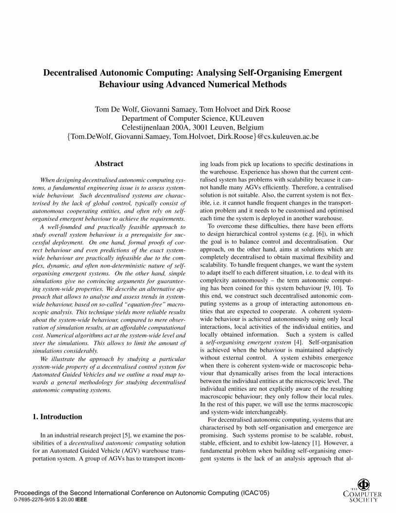
Figure 1. The AGV Simulator.
Because it is too expensive and often infeasible to apply
the analysis approach on a real AGV system, we developed
a realistic simulator1 for AGV systems that allows to ex-
ecute the simulations needed in the analysis approach de-
scribed in section 4. The screen-shot in figure 1 illustrates
the problem setting described above: the locations where
packets must be picked up are located at the left of the fig-
ure, the destinations are located at the right, and the network
in-between consists of stations and connecting segments on
which the AGVs can move. Segments are unidirectional,
i.e. an AGV can follow a segment in one direction. A bid-
irectional segment can be constructed with two overlapping
unidirectional segments. This facilitates the construction of
maps and minimises the possible collision regions. Packets
1http://www.cs.kuleuven.be/˜distrinet/taskforces/agentwise/agvsimulator/
are depicted as rectangular boxes and some of the AGVs
shown hold a packet, others do not.
3.2. A Self-Organising Emergent Solution
The AGV problem is a dynamic problem with non-
deterministic features (e.g. packets can arrive at any mo-
ment, AGVs can fail, obstacles can appear). The project
with our industrial partner [5] has shown that a solution
using a central server to control all AGVs cannot handle
these frequent changes efficiently. The central server has to
constantly monitor the warehouse and each AGV to detect
changes and react to them by steering each AGV. Because
AGVs are moving constantly, reacting on changes has to oc-
cur instantaneously. Therefore, the central server becomes
a bottleneck in the presence of frequent changes. As a con-
sequence, such a central solution is not scalable and can
only handle a limited number of AGVs. Also, the system
is not flexible when it has to be deployed, i.e. the system
needs to be customised and optimised each time it is de-
ployed in another warehouse. Therefore, in the context of
decentralised autonomic computing for larger and dynamic
AGV systems, a self-organising emergent solution in which
the AGVs adapt to the changing situations themselves by
only using locally obtained information, local interactions,
and local activity is promising. In the rest of this section,
a self-organising emergent solution is described, which is
only one of the large number of possible solutions. We do
not state that this is the perfect solution, it is only a test case.
Each AGV needs information to decide autonomously
where to move to on the network in order to reach an incom-
ing packet or a destination to drop a packet. This informa-
tion should be made available locally. To achieve this, we
use so-called artificial pheromones that propagate through
the network. Such pheromones are pieces of data that are
present in the network and, just like real pheromones, they
evaporate over time (i.e. older data disappears gradually).
When a location where packets arrive contains a packet, that
location will actively propagate pheromones through the
network. The pheromones are propagated between neigh-
bouring stations (i.e. only local interaction) in the direction
opposite to the direction in which the AGVs can move. A
pheromone includes information, such as the priority of the
packet, that is important for the AGVs to choose a packet.
Also, the distance from the station on which the pheromone
is located to the location of the packet is important inform-
ation. Therefore, when a pheromone propagates through a
segment, the cost of travelling over that segment is added to
the pheromone. This way, the distance is calculated during
the propagation process. All the pheromones in the network
form a gradient map for the AGVs to follow: on each sta-
tion, the pheromones indicate which outgoing segment is
the “best” to follow, i.e. the AGV chooses the segment in
Proceedings of the Second International Conference on Autonomic Computing (ICAC’05) 0-7695-2276-9/05 $ 20.00 IEEE

the direction of the closest packet and with the highest pri-
ority. Decisions are made one segment at a time, i.e. there
is no planning of a fixed path from source to destination.
When an AGV finally reaches a packet, it picks it up,
and follows another type of pheromone gradient, one that
is propagated from the destination locations. An AGV
chooses a segment to follow so that it can reach the destin-
ation of the packet it is holding via the shortest path. This
shortest path can be found because again the distance is cal-
culated during propagation of the pheromones and added to
the pheromone information at each station.
Note that this solution assumes the presence of infra-
structure on the stations, that can contain pheromone in-
formation and can actively propagate incoming pheromones
towards neighbouring stations. Also, the communication
bandwidth between the stations should allow this propaga-
tion through the entire network. In this paper we assume
that this infrastructure is present. Other solutions that do
not need this infrastructure can also be analysed with the
approach described in section 4.
3.3. Desired Guarantees
There are multiple requirements in an AGV system for
which guarantees are needed. To motivate our test case,
we consider an essential characteristic of self-organisation
which states that certain system-wide properties should be
maintained. For example, to achieve a constant throughput
of packets, the system should ensure that on average there is
always a fraction of the AGVs available to transport new in-
coming packets, while another fraction is busy transporting
packets. In the AGV case, with the lay-out of figure 1, the
system-wide property that reflects this requirement is the
distribution of the total number of AGVs between two situ-
ations: AGVs moving towards the pick up locations without
a packet and AGVs holding a packet and moving towards
the destination locations. An equal distribution needs to be
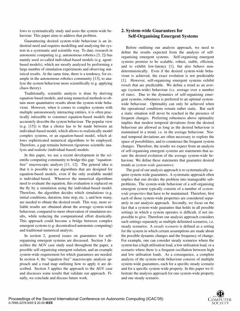
maintained. Considering the warehouse lay-out of figure
1, we can define two zones in which a certain situation is
desired (see figure 2):
• In Zone A the AGVs should be moving towards the
pick up locations and they should not hold a packet.
• In Zone B the AGVs should be moving towards the
drop off locations and they should hold a packet.
Note that there is an overlap between both zones at the
left and right of the factory lay-out. Because each AGV
can only be counted to be in one situation, the desired situ-
ations are used as a guide: an AGV in these overlap regions
is counted for zone A if the AGV does not hold a packet,
and for zone B if the AGV holds a packet. Note that also
AGVs in zone A could be holding a packet, as well as there
Zone B
Zone A
Figure 2. AGV Distribution between zones.
may be AGVs in zone B that aren’t. These situations are
undesirable, so we wish to avoid them.
Therefore, two guarantees are needed: an equal distribu-
tion between the two desired situations and a small num-
ber of AGVs in the undesirable situations. Because we
prefer robustness to optimality, it is allowed that at certain
points in time there is an unequal distribution and that some
AGVs are in an undesirable situation, as long as trends in
the system-wide behaviour guarantee the two requirements.
The analysis goal is to check if these requirements are
guaranteed for a specific solution and a specific steady scen-
ario. In this paper, we limit our analysis to the scenario with
a maximal system load. Consider the AGV case with the
lay-out shown in figure 1, with 10 AGVs, and with the as-
sumption that the pick up locations always contain a packet
(i.e. packets that are picked up are replaced immediately).
Furthermore, we assume that no other dynamic events can
occur (e.g. AGVs failing, AGVs added to the system, no
obstacles will appear, etc.). It is generally necessary and in-
teresting to investigate the effect of changes in this setting
on the dynamics of the system, but this is outside the scope
of the current paper.
To make the required guarantees concrete we quantify
them mathematically as follows. Two measures are con-
sidered. A first measure (E) represents the distribution
of AGVs between the two desired situations and a second
measure (S) represents the number of AGVs in the desired
situations. These system-wide measures can be calculated
from the number of AGVs in each situation:
NBAP : AGVs in zone A, holding a packet.
NBANP : AGVs in zone A, not holding a packet.
NBBP : AGVs in zone B, holding a packet.
NBBNP : AGVs in zone B, not holding a packet.
Proceedings of the Second International Conference on Autonomic Computing (ICAC’05) 0-7695-2276-9/05 $ 20.00 IEEE
We define the measure S to be the normalised sum of
AGVs in the desired situations. This yields:
S =NBANP + NBBP
NB(1)
In this equation, NB is the total number of AGVs. Accord-
ing to the requirements, S needs to be high.
From [8, 14, 2] we know that (spatial) entropy, defined
as
E =
−∑
1≤i≤N
pi ∗ log pi
log N, (2)
is suitable to reflect the spatial distribution of entities
between different states. Here pi is the probability that state
i occurs and∑
1≤i≤N pi = 1. Dividing by log N normal-
ises E to be between 0 and 1. Entropy is high (close to 1)
when the considered states have an equal probability to oc-
cur, and low (close to 0) when only a few of the states have
a high probability to occur.
To apply this measure to the distribution of AGVs, the
different states for the entropy measure are defined as the
desired situations for the AGVs. Consider the AGVs that
are already distributed between the desired situations. The
probability for such an AGV to be in one specific desired
situation at one moment in time is used as the probability
in the entropy equation. Then we can define the entropy
measure for the AGV example as:
E =−pANP log pANP − pBP log pBP
log 2(3)
with
pi =NBi
NBANP + NBBP
(i ∈ {ANP,BP}) (4)
and
pANP + pBP = 1 (5)
According to the requirements, E needs to be high be-
cause then there are approximately as many packet-carrying
AGVs in zone B as there are packet-less AGVs in zone A.
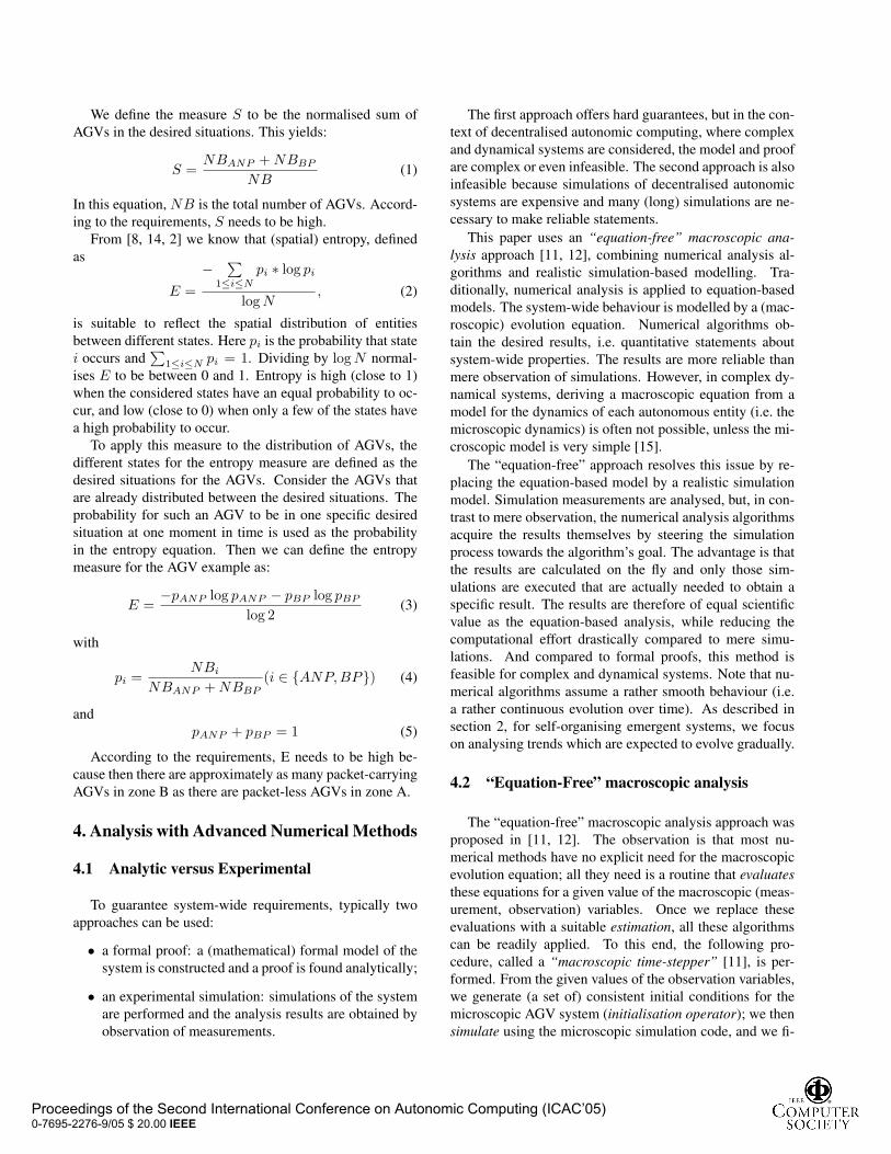
4. Analysis with Advanced Numerical Methods
4.1 Analytic versus Experimental
To guarantee system-wide requirements, typically two
approaches can be used:
• a formal proof: a (mathematical) formal model of the
system is constructed and a proof is found analytically;
• an experimental simulation: simulations of the system
are performed and the analysis results are obtained by
observation of measurements.
The first approach offers hard guarantees, but in the con-
text of decentralised autonomic computing, where complex
and dynamical systems are considered, the model and proof
are complex or even infeasible. The second approach is also
infeasible because simulations of decentralised autonomic
systems are expensive and many (long) simulations are ne-
cessary to make reliable statements.
This paper uses an “equation-free” macroscopic ana-
lysis approach [11, 12], combining numerical analysis al-
gorithms and realistic simulation-based modelling. Tra-
ditionally, numerical analysis is applied to equation-based
models. The system-wide behaviour is modelled by a (mac-
roscopic) evolution equation. Numerical algorithms ob-
tain the desired results, i.e. quantitative statements about
system-wide properties. The results are more reliable than
mere observation of simulations. However, in complex dy-
namical systems, deriving a macroscopic equation from a
model for the dynamics of each autonomous entity (i.e. the
microscopic dynamics) is often not possible, unless the mi-
croscopic model is very simple [15].
The “equation-free” approach resolves this issue by re-
placing the equation-based model by a realistic simulation
model. Simulation measurements are analysed, but, in con-
trast to mere observation, the numerical analysis algorithms
acquire the results themselves by steering the simulation
process towards the algorithm’s goal. The advantage is that
the results are calculated on the fly and only those sim-
ulations are executed that are actually needed to obtain a
specific result. The results are therefore of equal scientific
value as the equation-based analysis, while reducing the
computational effort drastically compared to mere simu-
lations. And compared to formal proofs, this method is
feasible for complex and dynamical systems. Note that nu-
merical algorithms assume a rather smooth behaviour (i.e.
a rather continuous evolution over time). As described in
section 2, for self-organising emergent systems, we focus
on analysing trends which are expected to evolve gradually.
4.2 “Equation-Free” macroscopic analysis
The “equation-free” macroscopic analysis approach was
proposed in [11, 12]. The observation is that most nu-
merical methods have no explicit need for the macroscopic
evolution equation; all they need is a routine that evaluates
these equations for a given value of the macroscopic (meas-
urement, observation) variables. Once we replace these
evaluations with a suitable estimation, all these algorithms
can be readily applied. To this end, the following pro-
cedure, called a “macroscopic time-stepper” [11], is per-
formed. From the given values of the observation variables,
we generate (a set of) consistent initial conditions for the
microscopic AGV system (initialisation operator); we then
simulate using the microscopic simulation code, and we fi-
Proceedings of the Second International Conference on Autonomic Computing (ICAC’05) 0-7695-2276-9/05 $ 20.00 IEEE

MACRO
MICRO
...XkX1 ... Xk+1
x1
xk
xk+1
xk+1+m
Xk+1+m
Simulations
init init
measure
measu
re
measure
Time
extrapolatio
n
step
Figure 3. Equation-Free Accelerated Simula-
tion over Time
nally measure the new values of the observation variables.
As such, the equation and its evaluation are replaced by the
simulation code and therefore the proposed method consti-
tutes a bridge between classical numerical analysis and mi-
croscopic (e.g. agent-based) simulation.
The described macroscopic time-stepper can be used to
accelerate the simulations significantly. Figure 3 illustrates
the basic idea. First an initial value x1 for the measured
variable is chosen by the analysis algorithm. Using this
value, a simulation is initialised with microscopic value(s)
X1 (i.e. init in figure 3), consistent with x1, and executed
for a certain duration. At some points in time, one meas-
ures the new value for the variable that is analysed (i.e.
measure in figure 3). This is repeated a number of times,
such that enough successive values xk are available for the
analysis algorithm to make the extrapolation step that skips
m time steps of simulation. This means that a new value
xk+1+m is estimated with extrapolation, using a number of
measured values (xk and xk+1 in figure 3). Starting from
this new value the process is repeated by initialising with
microscopic value(s) Xk+1+m. This acceleration over time
is called a projective integration algorithm. For a detailed
stability analysis, which allows to answer questions such
as how many observation values xk are needed to skip m
steps, we refer to [7]. Note that if the observation variables
behave stochastically, k may need to be increased to avoid
amplification of the statistical noise.
Simulations can also be accelerated in other ways. Sup-
pose we want to obtain the steady state behaviour, so we
look for values of the observation variables that remain con-
stant as time evolves. Instead of computing the time evolu-
tion until the system reaches this steady state, one can use
numerical methods that determine steady states in a more
direct and efficient way. Denote the macroscopic time-
stepper starting from an initial condition xi and perform-
ing a simulation for a fixed duration by Φ(xi). Denote the
initialisations
.....
simulation results
.....
simulate
simulate
xi
init
measure
analysis algorithm
code
parametersanalysis results
xi+1
MACRO
MICRO
Figure 4. Equation-Free Accelerated Simula-
tion guided by the analysis algorithm
value of the observation variable after this simulation as
xi+1 = Φ(xi). The steady state x∗ can then be computed
by solving the equation
Φ(x∗) − x∗ = 0 (6)
numerically, e.g. by Newton’s algorithm [16]. This iterat-
ive method generates consecutive approximations for the
steady state, which typically converge much faster to the
steady state than computing the time evolution through con-
secutive time steps.
Figure 4 summarises a more general view on the ap-
proach. First we supply to the analysis algorithm (e.g.
Newton’s algorithm) initial values (xi) for all the system-
wide variables under study. Then the init operator ini-
tialises a number of simulations accordingly, i.e. measuring
the system-wide variables after initialisation should equal
the given initial values. Because there are multiple ways to
initialise a simulation for the same value of a system-wide
variable, we need to initialise these “degrees of freedom”
randomly in multiple initialisations. Then the simulations
are executed for a predetermined duration. This duration
can be fixed or supplied by analysis algorithm. At the end,
one measures the averages of the values of the system-wide
variables (xi+1), which are given to the analysis algorithm
as a result. Then the analysis algorithm processes the new
results to obtain the next initial values (e.g. Newton: a guess
for the steady state). The cycle is repeated until the ana-
lysis algorithm has reached its goal (e.g. Newton: the steady
state). The algorithm decides on the configuration of the
simulations such as the initial conditions and the duration
of the simulations. Following the same principle, e.g. in the
presence of parameters, more general tasks, such as para-
meter optimisation or control can be performed as well [11].
Proceedings of the Second International Conference on Autonomic Computing (ICAC’05) 0-7695-2276-9/05 $ 20.00 IEEE

As such, a more focussed and accelerated simulation-based
analysis approach, guided by the analysis algorithm’s goal,
can be used to obtain more reliable results than mere obser-
vation of simulation results.
4.3 Road Map for Equation-Free MacroscopicAnalysis
There are a number of steps that have to be performed
for the equation-free approach to work. In this section we
give an overview of those steps:
1. Identification of observation variables. In the context
of self-organising emergent systems, the challenge is
to find variables which measure the system-wide prop-
erties under study. The properties to study are derived
from the system requirements. In other words, first a
quantification of the required emergent properties in
terms of measurable variables is needed.
2. Related system-wide variables. Are there other vari-
ables for system-wide properties that influence the
system-wide property under study? If so, then these
variables have to be incorporated into the analysis pro-
cess. Otherwise, the evolution of the system is not cor-
rectly and completely represented and analysed. The
underlying assumption of the equation-free analysis
approach is that a set of measurable variables can be
found that offer an adequate description of the macro-
scopic system dynamics. This means that the chosen
measurement variables are indeed the variables that
would appear in the macroscopic evolution equation.
In other words, when choosing system-wide variables,
we strive to reach a set of variables that reflect the mac-
roscopic degrees of freedom.
3. Micro-variables. For each system-wide variable, the
corresponding variables of the simulation at the level
of the individual entity in the system, that influence
this system-wide variable need to be identified.
4. Measurement operator. We need to know how to
calculate the system-wide variables from the micro-
variables in the simulation.
5. Initialisation operator. We need to define an operator
that allows to initialise the microscopic variables of the
simulation or multiple simulations to reflect the given
values for the system-wide variables. When there
are degrees of freedom in the initialisation, these are
initialised randomly and multiple simulation are con-
sidered to average this randomness.
6. Check the micro-macro scale separation. For the
equation-free approach to work and to be efficient, the
microscopic variables should evolve on a much faster
timescale than the macroscopic variables that determ-
ine the macroscopic evolution. Thus, changes in the
state of the individual entities in the system should be
fast compared to the evolution of the overall system
behaviour. If this would not be the case, then any error
introduced by our initialisation procedure could signi-
ficantly influence the results and hence create errors.
7. Define the different steady scenarios to analyse. As
explained earlier, we need to consider the possible
steady scenarios separately to allow systematic and
useful analysis. This step identifies system paramet-
ers that need to be modified in order to cover the range
of possible operational conditions for the system.
8. Choose an analysis algorithm. Once the previous steps
are successfully completed, an analysis algorithm can
be chosen. Depending on the kind of data and the
goals, e.g. finding steady state behaviour, optimising
values of system parameters, controlling the opera-
tional modus, one selects a suitable analysis algorithm
(e.g. projective integration, Newton’s method).
4.4. Underlying Assumptions
An important issue is if the analysis approach is gener-
ally applicable to decentralised autonomic computing sys-
tems. A thorough study of this issue is outside the scope
of this paper. However, at this moment, it seems that only
a separation of time scales between the macroscopic and
microscopic evolution is needed (see step 6 in road map).
When this assumption is valid, it implies that re-initialising
and restarting a simulation at arbitrary points produces res-
ults that are comparable to a single long simulation. Indeed,
in the presence of time-scale separation, initialisation errors
disappear quickly compared to the evolution of the system-
wide behaviour. For a review of the mathematical principles
that support this intuitive explanation, we refer to [12].
The main practical issue in applying the road map to
an arbitrary self-organising emergent system is to find a set
of macroscopic variables that correctly reflect the evolution
of the system-wide properties. This is far from trivial be-
cause an open issue for emergent systems is to understand
how the macroscopic behaviour is accomplished by the in-
dividual entities. Finding macroscopic variables, and how
they are measured from the microscopic state, requires de-
tailed knowledge of both the system under study and the
system-wide requirements. Besides a measurement oper-
ator, an initialisation operator is required that initialises
a microscopic simulation consistently with a macroscopic
variable. However, when these issues are resolved, a suc-
cessful application of the road map also results in new in-
sights on how the macroscopic behaviour is related to the
Proceedings of the Second International Conference on Autonomic Computing (ICAC’05) 0-7695-2276-9/05 $ 20.00 IEEE

behaviour of the individual entities. Moreover, in section
5.3, we show how to check if a set of macro-variables com-
pletely captures the evolution of the system-wide property.
5. Equation-Free Macroscopic Analysis of the
AGV System
5.1. Preliminary simulations
0
0.1
0.2
0.3
0.4
0.5
0.6
0.7
0.8
0.9
1
E=
entr
opy
0 500 1000 1500 2000 2500
time (seconds)
Figure 5. E in one AGV simulation run.
We first have to define which system-wide variables are
suited for macroscopic analysis (step 1 of road map). This
requires some preliminary simulations. We consider the
AGV case as described in section 3. The initial condi-
tion is given by an equal distribution of AGVs over the
two zones, and none is holding a packet. Since there
are 10 AGVs in total, the initial distribution is given by
NBANP = NBBNP = 5 and NBAP = NBBP = 0.
This results in an entropy E = 0, and a normalised sum
S = 0.5. (See formulas (1) and (3).) We perform a simula-
tion over 2500 time steps and measure E and S at each time
step. The simulator is written such that one time step cor-
responds to a logical duration of 1 second. The result for Eis shown in figure 5. We see a clear non-deterministic effect
in this variable, which is also true for S. Moreover, there
are discontinuous jumps, because the variable can only take
a discrete set of values.
However, if we perform the same simulation a large
number of times and average the results, we see that this
randomness smoothes out. Consider the same system, and
the same initial condition. Now, we perform N = 1000simulation runs instead of just one, and we report on the
values averaged over all runs, i.e. Eavg and Savg in figures
6(a) and 6(b). It is clear that, despite the non-deterministic
nature of one simulation, the averaged behaviour evolves
rather smoothly. Therefore, it is possible to make state-
ments about the average long-term values of entropy and
0
0.1
0.2
0.3
0.4
0.5
0.6
0.7
0.8
0.9
1
Eavg
0 500 1000 1500 2000 2500
time (seconds)
(a) average entropy
0
0.1
0.2
0.3
0.4
0.5
0.6
0.7
0.8
0.9
1
Savg
0 500 1000 1500 2000 2500
time (seconds)
(b) average sum
0
1
2
3
4
5
6
7
8
9
10
NB
PT
,avg
0 500 1000 1500 2000 2500
time (seconds)
(c) average number of packets in transport
Figure 6. Eavg, Savg, and NBPT,avg of a set of
N = 1000 runs of the AGV case as a functionof time.
normalised sum with numerical methods. In the rest of
our analysis, the average entropy Eavg and normalised sum
Savg are the system-wide observation variables.
Proceedings of the Second International Conference on Autonomic Computing (ICAC’05) 0-7695-2276-9/05 $ 20.00 IEEE

5.2. Macroscopic time-stepper
Once we have identified the system-wide variables of in-
terest, here Eavg and Savg , we need to determine other vari-
ables that might influence their values (step 2 from road
map). To achieve a one-to-one correspondence between
E, S and the variables NBAP , NBANP , NBBP and
NBBNP , we add the number of packets in transport NBPT
to the set of system-wide variables. Recall that a packet
is in transport if it is held by an AGV. The simulations
from section 5.1 show that the average of NBPT , denoted
by NBPT,avg, is also smooth (see figure 6(c)) and thus
suitable for our algorithms. Therefore, we add the aver-
aged variable NBPT,avg to our set of observation variables.
Note that the total number of AGVs is chosen to be constant.
So, for a set of N runs, these macroscopic variables are
completely determined by the variables NBAP , NBANP ,
NBBP and NBBNP , averaged over all runs. The precise
positions and internal states of each AGV are degrees of
freedom (steps 3 and 4 from road map).
We recall that the current state of each individual run
is limited to a discrete set of values for the entropy E,
the normalised sum S and the number of packets in trans-
fer NPBT , because changes in these values reflect that
one AGV has changed zone, or has picked up or de-
livered a packet. We denote all possible states by xi =(Ei, Si, NBPT,i). A complete initialisation operator (step
5 from road map) consists of two steps: first we need a
procedure to find the values of NBAP , NBANP , NBBP ,
NBBNP , given a particular state xi; and second, when av-
erage values Eavg , Savg , NBPT,avg and a number of runs
N are given, we need to find numbers Ni that indicate how
often state xi will be chosen as initial condition so that the
averages over all N runs equal the given average values
Eavg , Savg , and NBPT,avg. For a realistic simulation, the
distribution of the initial conditions over the possible states
should reflect the probability for the occurrence of that state.
Initialisation of one simulation. From equation (3) and
(5) one can derive:
E =−pBP log pBP − (1 − pBP ) log [1 − pBP ]
log 2(7)
It can easily be checked that this equation has two pos-
sible solutions for pBP , i.e. pBP1 and pBP2 = 1 − pBP1.
However, only one will fulfill the required constraints:
• NBPT = NBBP + NBAP
• NB = NBAP + NBBP + NBANP + NBBNP
• NBi ≥ 0(i ∈ {ANP,AP,BNP,BP})
• equation (1) and equation (3).
One solution pBP can be found numerically. If this solu-
tion does not comply with the constraints, then the other
solution, given by pBP2 = 1 − pBP1 will. Using the com-
plying solution for pBP and pANP = 1 − pBP , we can
calculate the NBi values:
NBBP = pBP ∗ NB ∗ S (8)
NBANP = pANP ∗ NB ∗ S (9)
NBAP = NBPT − NBBP (10)
NBBNP = NB − NBBP − NBANP
−NBAP − NBBNP (11)
Equation (10) assigns the remaining packets to the AGVs
in zone A that hold a packet. Then equation (11) just as-
signs the number of remaining AGVs to the last variable
NBBNP . Once the NBi values are calculated, there are
multiple initialisations possible because the exact AGV po-
sitions and the AGVs holding a packet are not determined.
These degrees of freedom are initialised randomly.
Initialisation of a set of runs. To define the initialisation
operator init completely, we need to solve the following
inverse problem: given values for Eavg , Savg , NBPT,avg,
find a set of N states, such that the averages are as specified.
In general, there are many solutions to this problem. For a
correct “equation-free” simulation, it is important to pick a
solution that is as realistic as possible.
First, we determine the probability of occurrence of each
state xi. To this end, we perform a long simulation of 50000steps. At each time step, we record the current state xi, and
obtain a histogram of occurrences. Then, the probability pi
of the system being in one of these states is approximated
by the number of occurrences of state xi, divided by the
number of time steps. These pi can be assumed to be the
fractions of time that the system is expected to be in state
xi. We then obtain a probability distribution for the macro-
scopic states. Note that we assume that the states xi cover
the whole spectrum of possible states and that, as time ap-
proaches infinity, the probabilities pi converge to a constant
limit. Our simulations confirm this as a valid assumption.
We need to choose the initial conditions for a simula-
tion as closely as possible to this distribution; otherwise,
we probably do not capture the true average behaviour. In-
deed, suppose that we initialise with a set of runs that has
the correct average, but that is initialised mainly with states
that are improbable. The results would be biased towards
the improbably initialised behaviour and thus meaningless
to interpret the real average behaviour. Therefore, we com-
pute weights wi, associated to each of the possible states of
the system, as follows. We require that the weights wi are
chosen such that they are as close as possible to the probab-
Proceedings of the Second International Conference on Autonomic Computing (ICAC’05) 0-7695-2276-9/05 $ 20.00 IEEE

ilities pi. This can be written as a minimisation problem,
minwi∈[0..1]
∑
i
|wi − pi|,
which is subject to the following constraints,
∑
i
wiEi = Eavg;∑
i
wiSi = Savg
∑
i
wiNBPT,i = NBPT,avg;∑
i
wi = 1.
These constraints indicate that the weighted averages
should be consistent with what we prescribed, and the
weights should be normalised. Then, we have assured that
we have a fraction wi of initial conditions for each of the
possible discrete states, such that both the distribution of
initial conditions is close to the pi-distribution, and the aver-
age initial entropy, sum and number of packets in transport
are as prescribed. Next, we need to assign initial conditions
to N number of runs. This is done by assigning Ni runs
with each initial condition/state xi such that
minNi
∑
i
|Ni − wiN |,
subject to the constraint
∑
i
Ni = N.
The minimisation requires that the fraction of runs initial-
ised with each state Ni/N is as close as possible to the frac-
tion wi, while fulfilling the constraint that their sum equals
N . Finally, in order that this set of runs has the correct av-
erages exactly, we weigh them with a factor αi = wiN/Ni.
This is easily seen by combining the constraints from the
two above minimisation problems. The two minimisation
problems can easily be solved using standard linear pro-
gramming methods [17].
Separation of scales. It is important for the equation-free
approach that the randomly initialised microscopic proper-
ties of the system, evolve much faster than the system-wide
variables (step 6 from road map). In our case, these vari-
ables include the exact position each AGV, whether they are
holding a packet or not, as well as the pheromone gradient
from the source and destination locations. It is clear that the
AGV movement, their pick ups and drop offs occur faster
than changes in Eavg , Savg, or NBPT,avg. We also ex-
pect the pheromone gradient to evolve quickly to its natural
state, so that this indeterminacy does not create artifacts.
5.3. Simulation with Re-initialisation
We will now check the validity of the macroscopic time-
stepper, i.e. validate that the chosen macroscopic variables
completely reflect the evolution of the system-wide beha-
viour. To this end, we perform a simulation using N =1000 runs, which have been initialised such that Eavg = 0,
Savg = 0.5 and NBPT,avg = 0. Note that all simulations
in this paper use the steady scenario described in section 3
(step 7 from road map). The simulation is performed over
250 time-steps, after which Eavg , Savg and NBPT,avg are
measured. To reduce the statistical noise, we measure these
variables as being averaged over the last 50 time-steps as
well as over all runs. We then re-initialise the simulation
immediately, following the lines of the previous section.
To compare with the preliminary results of section 5.1,
we performed 10 of these macroscopic time steps, such
that the total simulated time is again 2500 seconds, such
as in section 5.1. We remark that, at this stage, the sim-
ulations are not yet accelerated. The only difference with
the simulations in section 5.1 is that after each 250 time-
steps the simulation has been re-initialised. Figures 7(a),
7(b), and 7(c) show that these re-initialisations do not affect
the results significantly compared to the preliminary simu-
lation results (figures 6(a), 6(b), and 6(c)). The figures show
the values of Eavg, Savg and NBPT,avg at each time-step.
After each re-initialisation, we first see a steep transient.
This is due to the fact that the re-initialisation only ensures
that the macroscopic variables have been initialised consist-
ently. The microscopic states that are not accounted for are
initialised randomly. Therefore, an artificial fast evolution
of Eavg , Savg , and NBPT,avg is introduced which equilib-
rates quickly. This results in a sharp initial transient, which
disappears well before the end of the macroscopic time step
of size 250. Therefore, we conclude that the values of the
variables Eavg , Savg and NBPT,avg suffice to predict the
evolution of the system. This confirms that the macroscopic
time-stepper as constructed above accurately simulates the
system-wide behaviour.
5.4. A First Accelerated Result
We accelerate the simulations by using projective integ-
ration as an analysis algorithm (step 8 from road map). The
macroscopic variables that we introduced vary smoothly
over time, such that the extrapolation step can be done re-
liably. Due to the extrapolation steps, the computational
effort is reduced. We consider the following set-up: we per-
form a simulation run of 250 time-steps, as in the previous
section, after which we obtain the new values of the vari-
ables Eavg , Savg and NBPT,avg by averaging the simula-
tion results over the last 50 time steps (steps 201 to 250). We
also measure the macroscopic variables after 200 time-steps
Proceedings of the Second International Conference on Autonomic Computing (ICAC’05) 0-7695-2276-9/05 $ 20.00 IEEE

0
0.1
0.2
0.3
0.4
0.5
0.6
0.7
0.8
0.9
1
Eavg
250 500 750 1000 1250 1500 1750 2000 2250 2500
time (seconds)
re-init
accelerated
(a) average entropy
0
0.1
0.2
0.3
0.4
0.5
0.6
0.7
0.8
0.9
1
Savg
250 500 750 1000 1250 1500 1750 2000 2250 2500
time (seconds)
re-init
accelerated
(b) average sum
0
1
2
3
4
5
6
7
8
9
10
NB
PT
,avg
250 500 750 1000 1250 1500 1750 2000 2250 2500
time (seconds)
re-init
accelerated
(c) average number of packets in transport
Figure 7. Eavg, Savg, and NBPT,avg of a setof N = 1000 runs obtained with simple re-initialisation (re-init) and with projective in-
tegration (accelerated).
by averaging over steps 151 to 200. It is clear from figure 7
that the macroscopic time-step of 250 seconds is sufficiently
large, such that these measurements are not contaminated
by the re-initialisation transient. Using these two measure-
ments, we extrapolate over a time interval of length 250 and
re-initialise. This way, we have halved the computational
effort, since the simulations will now only be performed in
half of the time interval for which we obtain results. The
accelerated results are shown in figure 7.
Several observations can be made. First, it is clear that
the increased efficiency comes at a penalty in the accuracy.
In an extrapolation step, some accuracy is lost. It is im-
portant to note that this extrapolation error is mainly due to
the non-deterministic nature of the underlying simulation.
We expect that advanced techniques for variance reduction,
e.g. [18], can significantly improve these results, and we are
actively pursuing research in this direction. However, even
with this simple averaging strategy, we are already able to
halve the simulation time.
Second, as can be seen from the measurements in fig-
ure 6(a), the macroscopic variables approach a steady state.
This indicates that a numerical algorithm to determine this
steady state directly is preferably used (step 8 from road
map). The Newton algorithm (see section 4.2) is such an al-
gorithm which takes an arbitrary initial guess for the steady
state as input and converges to the real steady state. How-
ever, due to the rather large variance on the measurements,
we were unable to converge successfully, unless the error
tolerance for the Newton algorithm was set very low (2
digits of accuracy). The reason is that the extrapolation
steps used in Newton’s algorithm require a higher degree of
smooth behaviour than a projective integration over time as
described previously. We expect to remedy this in the near
future by using a suitable variance reduction technique, and
will report on this in a future publication.
6. Conclusion and Future Work
This paper describes a promising analysis approach that
allows to address a fundamental engineering issue for auto-
nomic decentralised systems, i.e. assessing the system-wide
behaviour of self-organising emergent systems. Due to the
complex, dynamic, and non-deterministic nature of such
systems, a formal or analytic proof and even predictions
of the exact behaviour are not feasible. Therefore, an al-
ternative road map to study trends in the system-wide be-
haviour is proposed, based on so-called ”equation-free”
macroscopic analysis techniques. Numerical analysis al-
gorithms are used to steer and accelerate the simulation pro-
cess. The main assumption is the presence of a separation in
time scales between the microscopic and macroscopic evol-
ution. Initial steps in the AGV case study show that this
technique can yield more reliable results about the system-
wide behaviour, compared to mere simulation observation
results, at an affordable computational cost.
Proceedings of the Second International Conference on Autonomic Computing (ICAC’05) 0-7695-2276-9/05 $ 20.00 IEEE
Several questions remain open, and constitute the basis
for future work. First, it is a challenge to alter the numerical
procedure in such a way that it uses suitable variance reduc-
tion techniques to obtain the level of smoothness that the
numerical algorithms require. This is necessary to success-
fully apply more advanced algorithms, such as bifurcation
tools to study parameter sensitivity. For example, the influ-
ence of a specific parameter on the system-wide behaviour,
e.g. the number of AGVs on the factory floor can signific-
antly influence the guarantees that can be given. Such a
parameter can then be used to control the system-wide be-
haviour by making sure that it stays in the range of values
that lead to desired behaviour. Secondly, additional steady
scenarios to analyse need to be considered (e.g. low utilisa-
tion load, frequent failure of AGVs, frequent occurrence of
obstacles, etc.). In general, one needs to identify the para-
meters that determine the conditions in which a system is
used, and analyse steady scenarios to cover the full range
of possibilities. Thirdly, we are actively investigating how
additional system-wide properties in the AGV case, such as
throughput, can be incorporated in the analysis. The iden-
tification of a set of problem-specific “key variables” still
needs to be done on a case-by-case basis. Once the pro-
cedure has been successfully applied to a range of systems,
we expect to obtain a set of useful guidelines for this cru-
cial step. Finally, the biggest challenge for the future is to
see to which extent this analysis approach can be integrated
into a systematic engineering approach for self-organising
emergent systems.
7. Acknowledgements
G. Samaey is a Research Assistant of the Fund for Sci-
entific Research – Flanders (FWO). This work is suppor-
ted by grants FWO G.0130.03, IUAP/V/22 (Belgian Fed-
eral Science Policy Office) (G. Samaey, D. Roose), and by
the K.U.Leuven research council as part of the Concerted
Research Action on Agents for Coordination and Control -
AgCo2 (T. De Wolf, T. Holvoet).
References
[1] R. J. Anthony. Emergence: A paradigm for robust and scal-
able distributed applications. In Proceedings of IEEE Inter-
national Conference on Autonomic Computing (ICAC’04),
pages 132–139, New York, May 2004.
[2] T. Balch. Hierarchic social entropy: An information theor-
etic measure of robot group diversity. Autonomous Robots,
8:209–237, 2000.
[3] T. Balch and R. C. Arkin. Communication in reactive mul-
tiagent robotic systems. Autonomous Robots, 1(1):27–52,
1995.
[4] T. De Wolf and T. Holvoet. Emergence and Self-
Organisation: a statement of similarities and differences. In
Proceedings of the Second International Workshop on En-
gineering Self-Organising Applications, pages 96–110, July
2004.
[5] Egemin and DistriNet. Emc2: Egemin modular controls
concept,. IWT-funded project with participants: Egemin
(http://www.egemin.be) and DistriNet (research group of
K.U.Leuven). Started on 1 March 2004, ending on 28 Feb-
ruary 2006.
[6] M. P. Fromherz, L. S. Crawford, C. Guettier, and Y. Shang.
Distributed adaptive constrained optimization for smart mat-
ter systems. In Proceedings of AAAI Spring Symposium on
Intelligent Embedded and Distributed Systems, 2002.
[7] C. Gear and I. Kevrekidis. Projective methods for stiff
differential equations: problems with gaps in their eigen-
value spectrum. SIAM Journal on Scientific Computing,
24(4):1091–1106, 2003.
[8] S. Guerin and D. Kunkle. Emergence of constraint in
self-organizing systems. Nonlinear Dynamics, Psychology,
and Life Sciences, 8(2):131–146, April 2004. (available at
http://www.redfish.com/).
[9] IBM. Autonomic Computing Manifesto: IBM’s Perspective
on the State of Information Technology. IBM, 2001. (online
at http://www.research.ibm.com/autonomic/manifesto/).
[10] J. O. Kephart and D. M. Chess. The vision of autonomic
computing. IEEE Computer Magazine, 36(1):41–50, Janu-
ary 2003.
[11] I. G. Kevrekidis, C. W. Gear, and G. Hummer. Equation-
free: The computer-assisted analysis of complex, multiscale
systems. AIChE Journal, 50(7):1346 – 1355, 2004.
[12] I. G. Kevrekidis, C. W. Gear, J. M. Hyman, P. G. Kevrekidis,
O. Runborg, and C. Theodoropoulos. Equation-free, coarse-
grained multiscale computation: enabling microscopic sim-
ulators to perform system-level analysis. Communications
in Mathematical Sciences, 1(4):715 – 762, December 2003.
(available online at http://www.intlpress.com/CMS/).
[13] U. Nehmzow. Quantitative analysis of robot-environment
interaction - towards scientific mobile robotics. J. Robotics
and Autonomous Systems, 44:55–68, 2003.
[14] H. V. D. Parunak and S. Brueckner. Entropy and Self-
Organization in Multi-Agent Systems. In J. P. Muller, E. An-
dre, S. Sen, and C. Frasson, editors, Proceedings of the Fifth
International Conference on Autonomous Agents, pages
124–130, Montreal, Canada, 2001. ACM Press. (available
at citeseer.ist.psu.edu/parunak01entropy.html).
[15] H. V. D. Parunak, R. Savit, and R. L. Riolo. Agent-based
modeling vs. equation-based modeling: A case study and
users’ guide. In MABS, pages 10–25, 1998. (online at
http://www.erim.org/˜vparunak).
[16] W. H. Press, B. P. Flannery, S. A. Teukolsky, and W. T. Vet-
terling. Numerical Recipes in C: The Art of Scientific Com-
puting. Cambridge University Press, Cambridge, 2nd edi-
tion, 1992.
[17] W. Winston. Operations research: applications and al-
gorithms. International Thomson Publishing, Belmont, CA,
3rd edition, 1994.
[18] Y. Zou and R. Ghanem. A multiscale data assimilation with
the ensemble kalman filter. Multiscale modelling and simu-
lation, 3(1):131–150, 2004.
Proceedings of the Second International Conference on Autonomic Computing (ICAC’05) 0-7695-2276-9/05 $ 20.00 IEEE
Top Related