


Languages
Pages
Legal


Data Analysis

Basic Problem
• There is a population whose properties we are interested in and wish to quantify statistically: mean, standard deviation, distribution, etc.
• The Question – Given a sample, what was the random system that generated its statistics?

Central Limit Theorem
• If one takes random samples of size n from a population of mean and standard deviation then as n gets large, approaches the normal distribution with mean and standard deviation
• is generally unknown and often replaced by the sample standard deviation s resulting in , which is termed the Standard Error of the sample.
n
X
ns

Example

Normal distribution

Critical Values for Confidence Levels
1- .80 .90 .95 .99 0.20 0.10 0.05 0.01/2 0.10 .05 .025 0.005z/2 1.28 1.64 1.96 2.58

Confidence Interval for Mean(large sample size)
)(2/ nszX
)(2/ XSEzX
OR
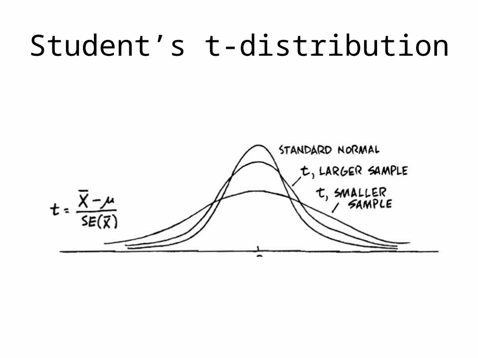
Student’s t-distribution

Critical Values for Confidence Levelst-distribution
1- .80 .90 .95 .99 0.20 0.10 0.05 0.01/2 0.10 .05 .025 0.005d.f. = 1 3.09 6.31 12.71 63.66d.f. = 10 1.37 1.81 2.23 4.14d.f. = 30 1.31 1.70 2.04 2.75d.f. = 1.28 1.65 1.96 2.58

Confidence Interval for Mean(small sample size, t-distribution)
)(2/ nstX
)(2/ XSEtX
OR

Comparing Population Means
)( 212/2121 XXSEtXX
2
22
1
21
21 )(n
s
n
sXXSE
2121
11)(
nnsXXSE pool
Pooled Variance
Unequal Variance

Hypothesis Testing (t-test)
• Null Hypothesis – differences in two samples occurred purely by chance
• t statistic = (estimated difference)/SE• Test returns a “p” value that represents the
likelihood that two samples were derived from populations with the same distributions
• Samples may be either independent or paired
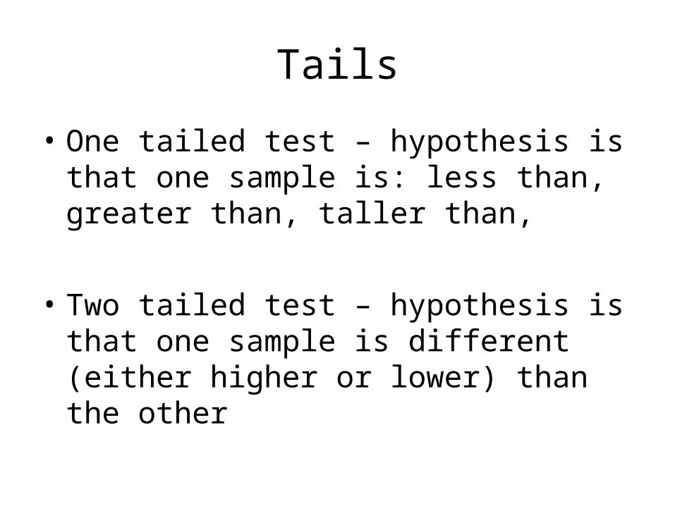
Tails
• One tailed test – hypothesis is that one sample is: less than, greater than, taller than,
• Two tailed test – hypothesis is that one sample is different (either higher or lower) than the other

Paired Test
• Samples are not independent• Much more robust test to determine
differences since all other variables are controlled
• Analysis is performed on the differences of the paired values
• Equivalent to Confidence interval for the mean

Paired Samples – New Site

TSS Concentrations vs. Time

BMP Performance Comparison
• Commonly expressed as a % reduction in concentration or load– Highly dependent on influent concentration– Potentially ignores reduction in volume (load)
• May lead to very large differences in pollutant reduction estimates
• Preferable to compare discharge concentrations

Effect of TSS Influent Concentration
-100%
-80%
-60%
-40%
-20%
0%
20%
40%
60%
80%
100%
0 100 200 300 400 500 600
Influent Concentration
% R
emov
al
Swale
Strip
Detention
Sand Filter
Wet Pond

Sand Filter - TSS
y = 0.0046x + 7.4242
R2 = 0.0037
0
50
100
150
200
250
300
350
400
0 100 200 300 400 500
TSS Influent (mg/L)
TSS
Eff
luen
t (m
g/L)

Comparison of Effluent Quality

Exercise
• Calculate average concentrations for each constituent for the two watersheds
• Determine whether any concentrations are significantly different, report p value for null hypothesis
• Calculate average effluent concentrations for the two BMPs and determine whether they are different from the influent concentrations – p values
• Compare effluent concentrations for the two BMPs and determine whether one BMP is better than the other for a particular constituent.
Top Related