


Languages
Pages
Legal


d
Boundary Element Method (BEM)
Zhicheng Wang
Jonathan Sant’anna Garcez Nobrega
Eunnam Ahn
Kien Tran
Lihe Xiu
Livio Yang Santos
1EGEE 520 Mathematical Modeling of Energy & Geo-environmental Systems

Boundary Element Method (BEM) 2
Contents1. Introduction
2. Historical Perspective
3. General Principles
4. Governing Equations
5. Hand-Calculation Example
6. Numerical Example
7. Example Applications

Boundary Element Method (BEM) 3
Contents1. Introduction
2. Historical Perspective
3. General Principles
4. Governing Equations
5. Hand-Calculation Example
6. Numerical Example
7. Example Applications

Boundary Element Method (BEM) 4
1. Introduction
Analytical Solution
• Can obtained for few specific problems with simple BCs
• Satisfy both DE and BCs
Numerical Solution
• Applicable for realistic scenario of practical engineering problems (approximate solutions)
• Satisfy one of the two (DE or BCs) and minimize the error in satisfying the other one.
• Boundary Element Method (BEM): satisfy the DE exactly and minimize error in the satisfaction of BCs.
Nearly all physical phenomena occurring in nature can be describe by DEs and BCs.

Boundary Element Method (BEM) 5
1. Introduction: The Idea of BEM• Foundation idea of BEM came from Trefftz (1926), that
we can approximate the solution to a PDE by looking at
the solution to the PDE on the boundary and then use
that information to find the solution inside the domain.
Discretization into linear elements for problems of flow past cylinder [Gernot Beer et al. (2008)]
• As a consequence, the number of discretized elements
is way less than FEM or FDM.
• BEM can be applied for potential problems governed
by a DE that satisfied the Laplace equation or
behaviors that has relating fundamental solutions:
fluid flow, torsion of bars, diffusion and steady state
heat conduction…
• Also useful for problems with complicated geometries,
infinite domain problems.
Boundary Element Method (BEM) 6
1. Introduction: Advantages of BEMReduction of problem dimension by 1.
• Less data preparation time.
• Easier to change the applied mesh.
No approximations imposed on the solution at interior point.
• High accuracy.• Able to modeling
problems of rapidly changing stresses.
• Faster compute time and less storage.
Uses less number of nodes and elements.
• Filter out unwanted information, focus on section of the domain of interested.
• Further reduces compute time.
Internal points of the domain are optional.

Boundary Element Method (BEM) 7
1. Introduction: Disadvantages of BEM
• For non-linear problems, the interior must be modelled, especially in non-linear material problems.
• Poor for thin structures 3-D analysis, due to large surface/volume ratio and the close proximity of nodal points on either side of the structure thickness. Causing inaccuracies in the numerical integrations.
• Requires explicit knowledge of a fundamental solution of the PDE.
• The solution matrix resulting from the BE formulation is unsymmetric and fully populated with non-zero coefficients, this means that the entire BE solution matrix must be saved in the computer core memory.

Boundary Element Method (BEM) 8
FEM vs. BEM
Fedele F. et al. (2005)
• Discretization of whole domain • Discretization of boundary
• Good on finite domains • Good on infinite or semi-infinite domains
• Approximates interior point solution (u) & BCs solution (q) must be found from u and approximation of q may not be as accurate
• Approximates BCs solution (q) & interior point solution (u) approximation of q is accurate
• Requires no prior knowledge of solution • Requires knowledge of PDE solution
• Solves most linear second-order PDEs • Can be difficult to solve inhomogeneous or nonlinear problems
Boundary Element Method (BEM) 9
Contents1. Introduction
2. Historical Perspective
3. General Principles
4. Governing Equations
5. Hand-Calculation Example
6. Numerical Example
7. Example Applications
Boundary Element Method (BEM) 10
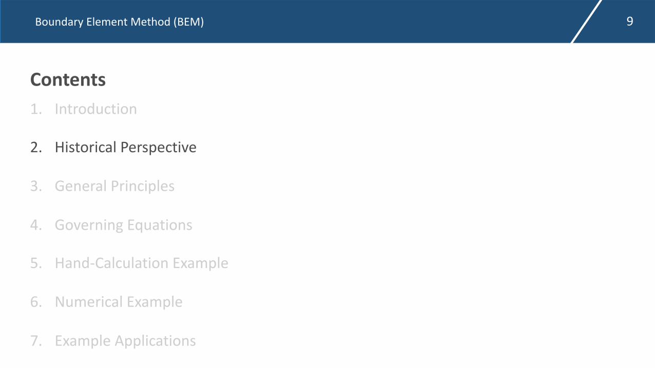
2. Historical Perspective• C. F. Gauss (1813)• Developed the Divergence Theorem.
• G. Green (1828)• Wrote a famous essay on the application of mathematical analysis to the theories of
electricity and magnetism.
Boundary Element Method (BEM) 11
2. Historical Perspective• E. I. Fredholm (1903)• Proved the existence and uniqueness of solution of the linear integral equation.
• M. A. Jaswon and A. R. Ponter (1963)• First formulated 2D potential problem in terms of a direct Boundary Integral
Equation (BIE) and solved it numerically.

Boundary Element Method (BEM) 12
2. Historical Perspective• F. J. Rizzo (1967)• Extended the work into the 2D elastostatic case.
• T. A. Cruse and F. J. Rizzo (1968)• Extended the work into 2D elastodynamics case.
Boundary Element Method (BEM) 13
2. Historical Perspective• P. K. Banerjee and R. Butterfield (1975)• Coined the term “Boundary Element Method” in an attempt to make an analogy
with Finite Element Method (FEM).
• C. A. Brebbia (1978)• Published the first textbook on BEM, ‘The boundary Element Method for Engineers’.
• From late 1970s, the number of journal articles shows an exponential grow rate.

Boundary Element Method (BEM) 14
Contents1. Introduction
2. Historical Perspective
3. General Principles
4. Governing Equations
5. Hand-Calculation Example
6. Numerical Example
7. Example Applications

Boundary Element Method (BEM) 15
3. General Principles: Mathematical Foundations1. Unitary impulse function
Boundary Element Method (BEM) 16
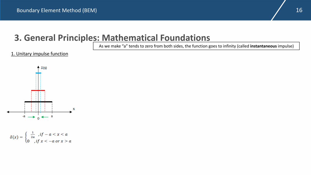
3. General Principles: Mathematical Foundations1. Unitary impulse function
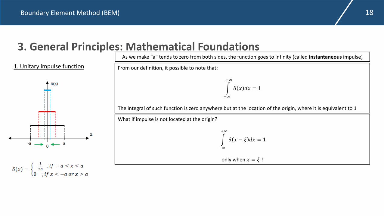
As we make “a” tends to zero from both sides, the function goes to infinity (called instantaneous impulse)
Boundary Element Method (BEM) 17
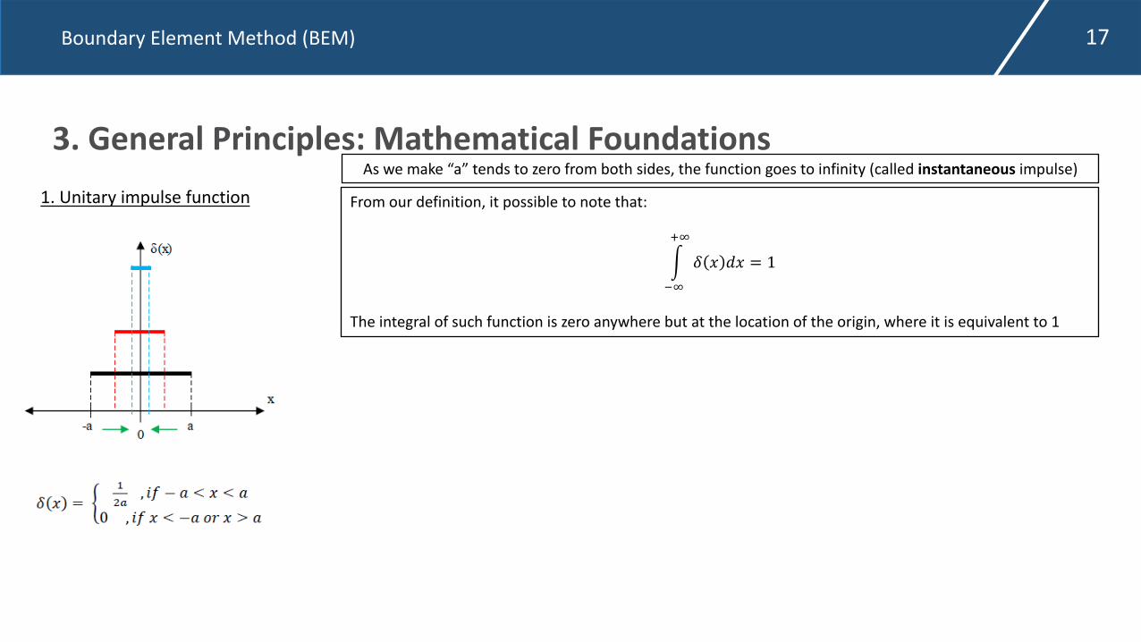
3. General Principles: Mathematical Foundations1. Unitary impulse function
As we make “a” tends to zero from both sides, the function goes to infinity (called instantaneous impulse)
From our definition, it possible to note that:
!"#
$#
% & '& = 1
The integral of such function is zero anywhere but at the location of the origin, where it is equivalent to 1
Boundary Element Method (BEM) 18
3. General Principles: Mathematical Foundations1. Unitary impulse function
As we make “a” tends to zero from both sides, the function goes to infinity (called instantaneous impulse)
From our definition, it possible to note that:
!"#
$#
% & '& = 1
The integral of such function is zero anywhere but at the location of the origin, where it is equivalent to 1
What if impulse is not located at the origin?
!"#
$#
% & − + '& = 1
only when & = + !

Boundary Element Method (BEM) 19
3. General Principles: Mathematical Foundations1. Unitary impulse function
As we make “a” tends to zero from both sides, the function goes to infinity (called instantaneous impulse)
From our definition, it is possible to note that:
!"#
$#
% & '& = 1
The integral of such function is zero anywhere but at the location of the origin, where it is equivalent to 1
What if impulse is not located at the origin?
!"#
$#
% & − + '& = 1
only when & = + !
Now we are able to understand the sifting property:
!"#
$#
% + − & ,(+)'+ = ,(&)
Attention: we are changing the domain of integration from & /0 +
Boundary Element Method (BEM) 20
3. General Principles: Mathematical Foundations2. Green’s function
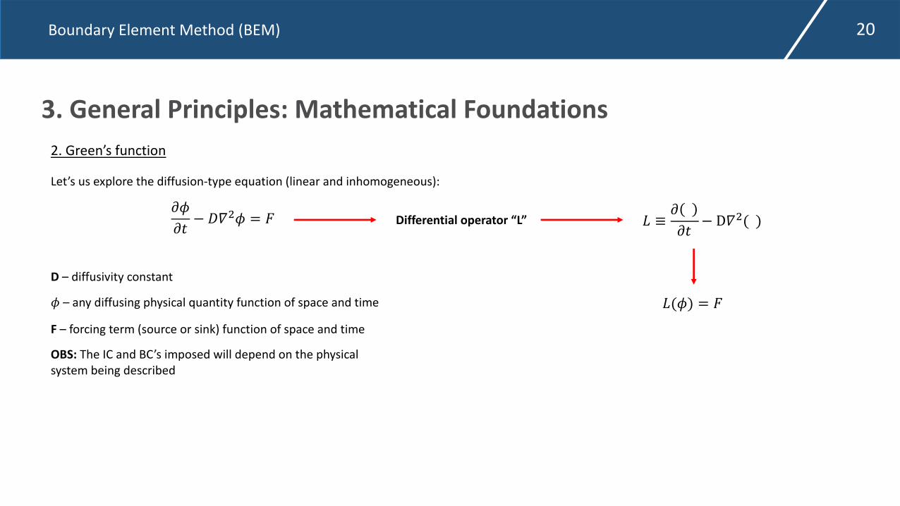
Let’s us explore the diffusion-type equation (linear and inhomogeneous):
!"!# − %&
'" = )
" – any diffusing physical quantity function of space and time
F – forcing term (source or sink) function of space and time
OBS: The IC and BC’s imposed will depend on the physical system being described
Differential operator “L” * ≡ !!# − D&'( )
*(") = )D – diffusivity constant
Boundary Element Method (BEM) 21
3. General Principles: Mathematical Foundations2. Green’s function
Let’s us explore the diffusion-type equation (linear and inhomogeneous):
!"!# − %&
'" = )
" – any diffusing physical quantity function of space and time
F – forcing term (source or sink) function of space and time
OBS: The IC and BC’s imposed will depend on the physical system being described
Differential operator “L” * ≡ !!# − D&'( )
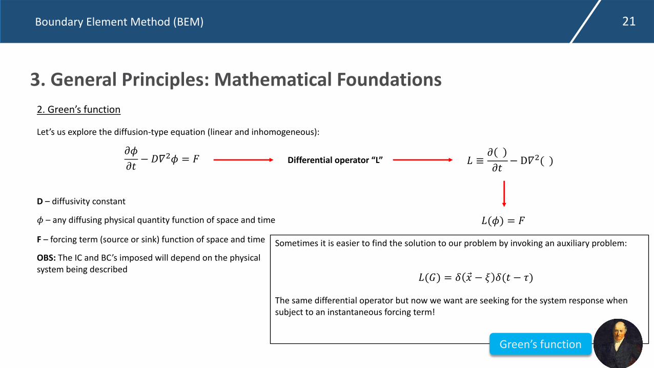
*(") = )Sometimes it is easier to find the solution to our problem by invoking an auxiliary problem:
The same differential operator but now we want are seeking for the system response when subject to an instantaneous forcing term!
*(/) = 0 2⃗ − 3 0(# − 4)
Green’s function
D – diffusivity constant

Boundary Element Method (BEM) 22
3. General Principles: Mathematical Foundations2. Green’s function
Typically, we call the “Free Space Green’s Function” the solution that only satisfies the differential operator
When working with the diffusion-type equation, the Green’s function is just a Gaussian function:
!(#, %; ', () = 1, 4.(% − ()
0#1 − # − ' 2
4,2(% − ()
Caution: function is not well defined at (', ()
Boundary Element Method (BEM) 23
3. General Principles: Mathematical Foundations
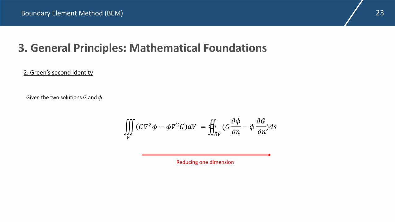
2. Green’s second Identity
!"
#$%& − &$%# () =+,"(# .&./ − &
.#./)(1
Given the two solutions G and &:
Reducing one dimension
Boundary Element Method (BEM) 24
Contents1. Introduction
2. Historical Perspective
3. General Principles
4. Governing Equations
5. Hand-Calculation Example
6. Numerical Example
7. Example Applications
Boundary Element Method (BEM) 25
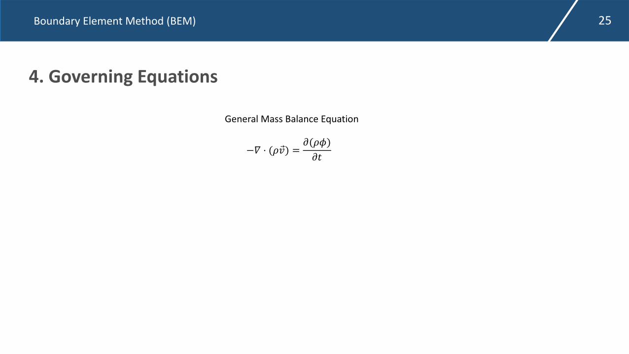
4. Governing Equations
−" ⋅ (%'⃗) = *(%+)*,
General Mass Balance Equation
Boundary Element Method (BEM) 26
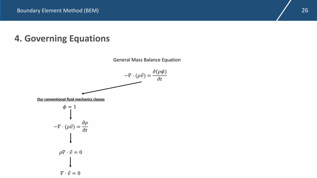
4. Governing Equations
−" ⋅ (%'⃗) = *(%+)*,
General Mass Balance Equation
+ = 1Our conventional fluid mechanics classes
−" ⋅ (%'⃗) = *%*,
%" ⋅ '⃗ = 0
" ⋅ '⃗ = 0

Boundary Element Method (BEM) 27
4. Governing Equations
−" ⋅ (%'⃗) = *(%+)*,
General Mass Balance Equation
+ = 1Our conventional fluid mechanics classes
−" ⋅ (%'⃗) = *%*,
%" ⋅ '⃗ = 0
" ⋅ '⃗ = 0
Fluid flow through porous media
We need a “bridge” that will help us to make our equation suitable to porous media flow (constitutive equation)
'⃗ = −/0 "1
Boundary Element Method (BEM) 28
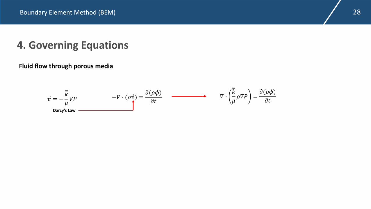
4. Governing Equations
−" ⋅ (%'⃗) = *(%+)*,
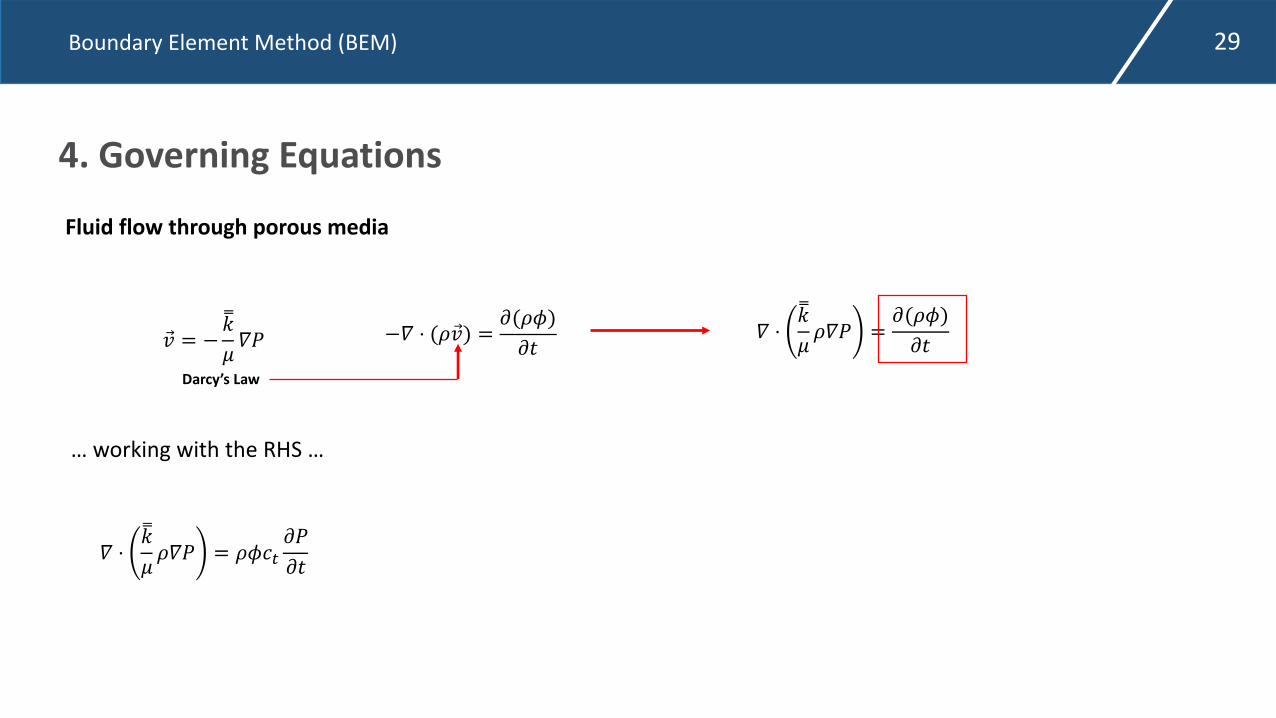
Fluid flow through porous media
'⃗ = −-./ "0
Darcy’s Law
" ⋅-./ %"0 = *(%+)
*,
Boundary Element Method (BEM) 29
4. Governing Equations
−" ⋅ (%'⃗) = *(%+)*,
Fluid flow through porous media
'⃗ = −-./ "0
Darcy’s Law
" ⋅-./ %"0 = *(%+)
*,
… working with the RHS …
" ⋅-./ %"0 = %+12
*0*,
Boundary Element Method (BEM) 30
4. Governing Equations
−" ⋅ (%'⃗) = *(%+)*,
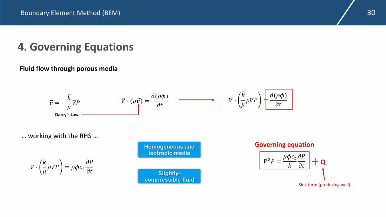
Fluid flow through porous media
'⃗ = −-./ "0
Darcy’s Law
" ⋅-./ %"0 = *(%+)
*,
… working with the RHS …
" ⋅-./ %"0 = %+12
*0*,
Homogeneous and isotropic media
Slightly-compressible fluid
"30 = /+12.
*0*,
Governing equation
Q
Sink term (producing well)

Boundary Element Method (BEM) 31
4. Governing EquationsIntegral solution protocol – the basis of Boundary Element Method
Writing in terms of the differential operator “L”
Dimensionless variables!"# = %&'(
)*#*+ + - !"#. −
*#.*+.0
= -.
1 ≡ !"( ) − *( )*+.0 1 #. = -.
By recognizing the fundamental solution of L as “G”:
1 5 ≡ !"5 − *5*+.0
= 6 7. − ξ 6(+.0 − 9)
Boundary Element Method (BEM) 32
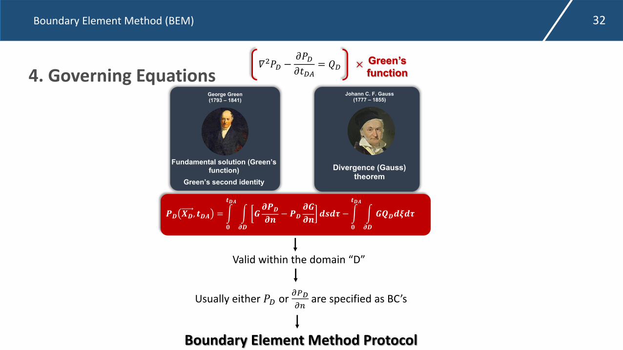
4. Governing Equations
!" #", %"& = ()
%"&(*"
+*!"*, − !"*+*, ./.0 − (
)
%"&(*"
+1".2.0
George Green (1793 – 1841)
Fundamental solution (Green’s function)
Green’s second identity
Johann C. F. Gauss (1777 – 1855)
Divergence (Gauss) theorem
Green’s function
3456 −7567869
= :6
Valid within the domain “D”
Boundary Element Method Protocol
Usually either 56 or ;<=;> are specified as BC’s
Boundary Element Method (BEM) 33
4. Governing Equations
!" #", %"& = (
)
%"&
(
*"
+*!"
*,− !"
*+
*,./.0 − (
)
%"&
(
*"
+1".2.0
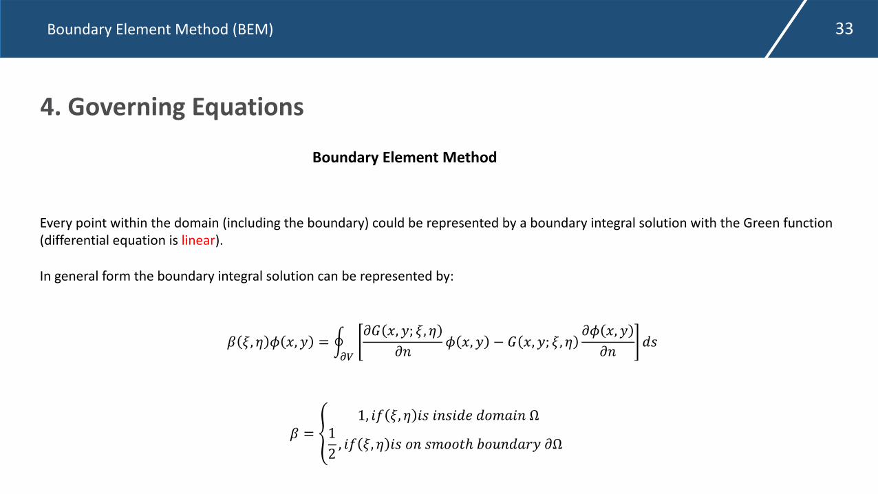
Boundary Element Method
Every point within the domain (including the boundary) could be represented by a boundary integral solution with the Green function (differential equation is linear).
In general form the boundary integral solution can be represented by:
3 4, 5 6 7, 8 = 9:;
<= 7, 8; 4, 5
<?6 7, 8 − = 7, 8; 4, 5
<6 7, 8
<?@A
3 = B
1, DE 4, 5 DA D?AD@F @GHID? Ω
1
2, DE 4, 5 DA G? AHGGLℎ NGO?@IP8 <Ω
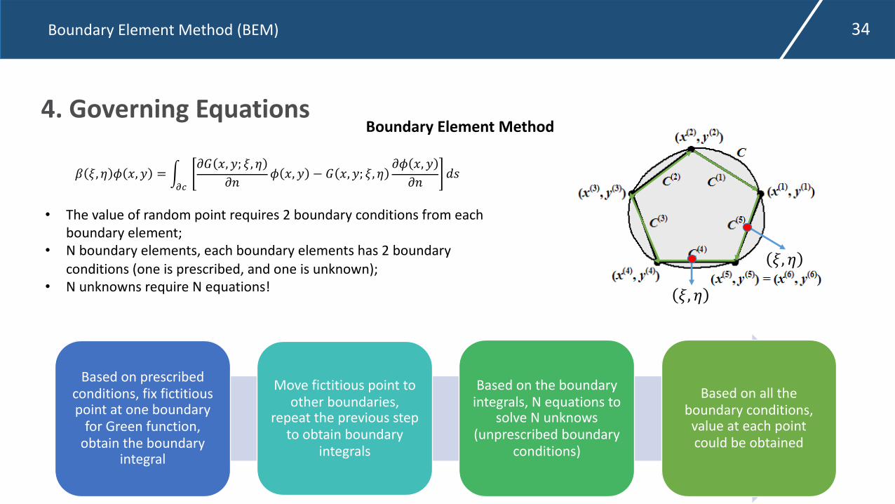
Boundary Element Method (BEM) 34
4. Governing Equations
Based on prescribed conditions, fix fictitious point at one boundary
for Green function, obtain the boundary
integral
Move fictitious point to other boundaries,
repeat the previous step to obtain boundary
integrals
Based on the boundary integrals, N equations to
solve N unknows (unprescribed boundary
conditions)
Based on all the boundary conditions,
value at each point could be obtained
!, #
!, #
$ !, # % &, ' = )*+
,- &, '; !, #,/ % &, ' − - &, '; !, # ,% &, '
,/ 12
• The value of random point requires 2 boundary conditions from each boundary element;
• N boundary elements, each boundary elements has 2 boundary conditions (one is prescribed, and one is unknown);
• N unknowns require N equations!
Boundary Element Method
Boundary Element Method (BEM) 35
Contents1. Introduction
2. Historical Perspective
3. General Principles
4. Governing Equations
5. Hand-Calculation Example
6. Numerical Example
7. Example Applications

Boundary Element Method (BEM) 36
5. Hand-Calculation Example
1
3
2 4
!"!# = 0" =?
!"!# = 0" =?
!"!# =?" = 1.0
4 boundaries; 4 B.C. given
!"!# =?" = 0
Imagine inside a fluid flow field and a square domain exists. 2 boundaries are specified with flow potential and 2 boundaries are specified with the )*)+ (which could be considered as velocity given). What is the other B.C. on each boundary?
Boundary Element Method (BEM) 37
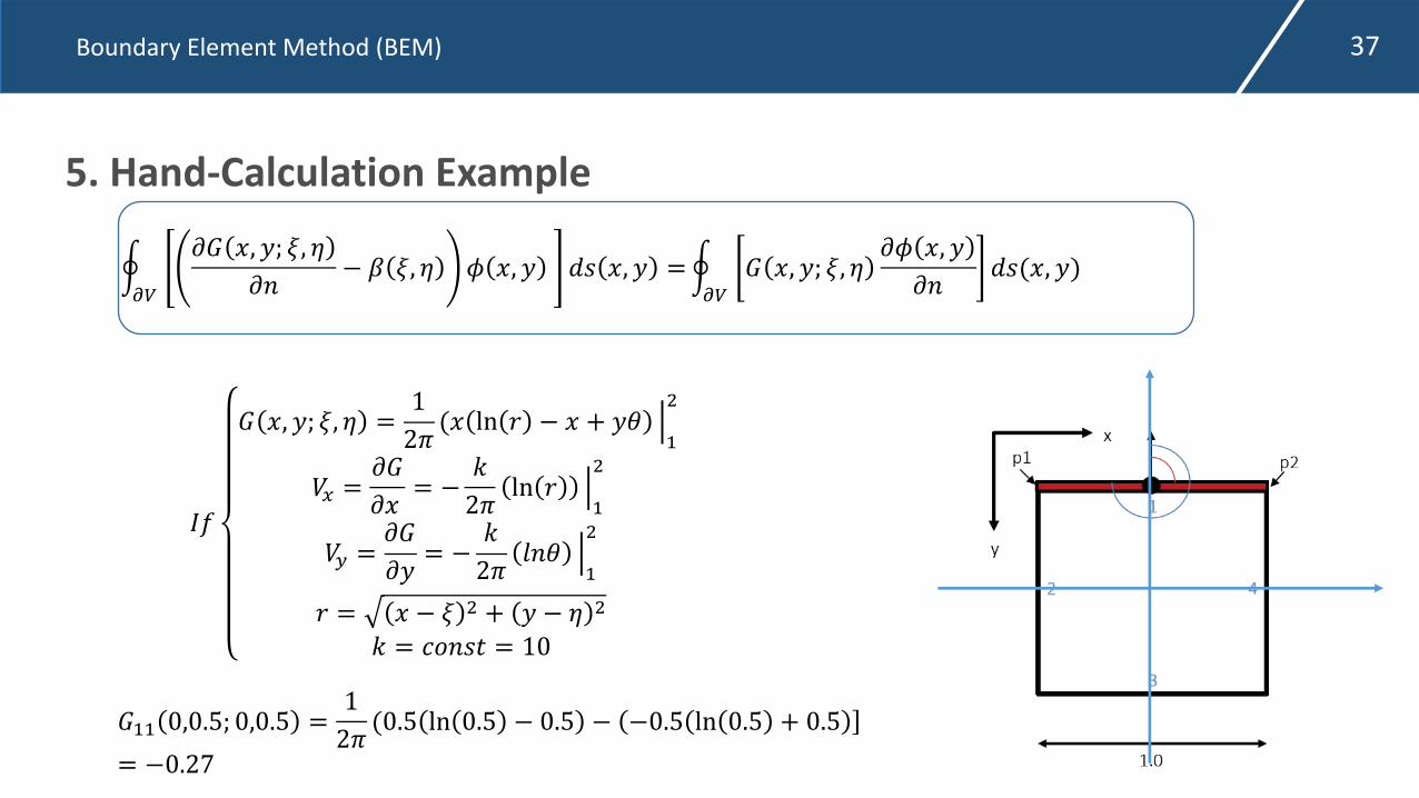
5. Hand-Calculation Example
!"#
$% &, (; *, +
$,− . *, + / &, ( 01 &, ( =!
"#% &, (; *, +
$/ &, (
$,01(&, ()
56
% &, (; *, + =1
29(& ln < − & + (> ?
@
A
BC =$%
$&= −
D
29ln < ?
@
A
BE =$%
$(= −
D
29F,> ?
@
A
< = & − * A + ( − + A
D = GH,1I = 10
%@@ 0,0.5; 0,0.5 =1
29(0.5 ln 0.5 − 0.5 − −0.5 ln 0.5 + 0.5
= −0.27
Boundary Element Method (BEM) 38
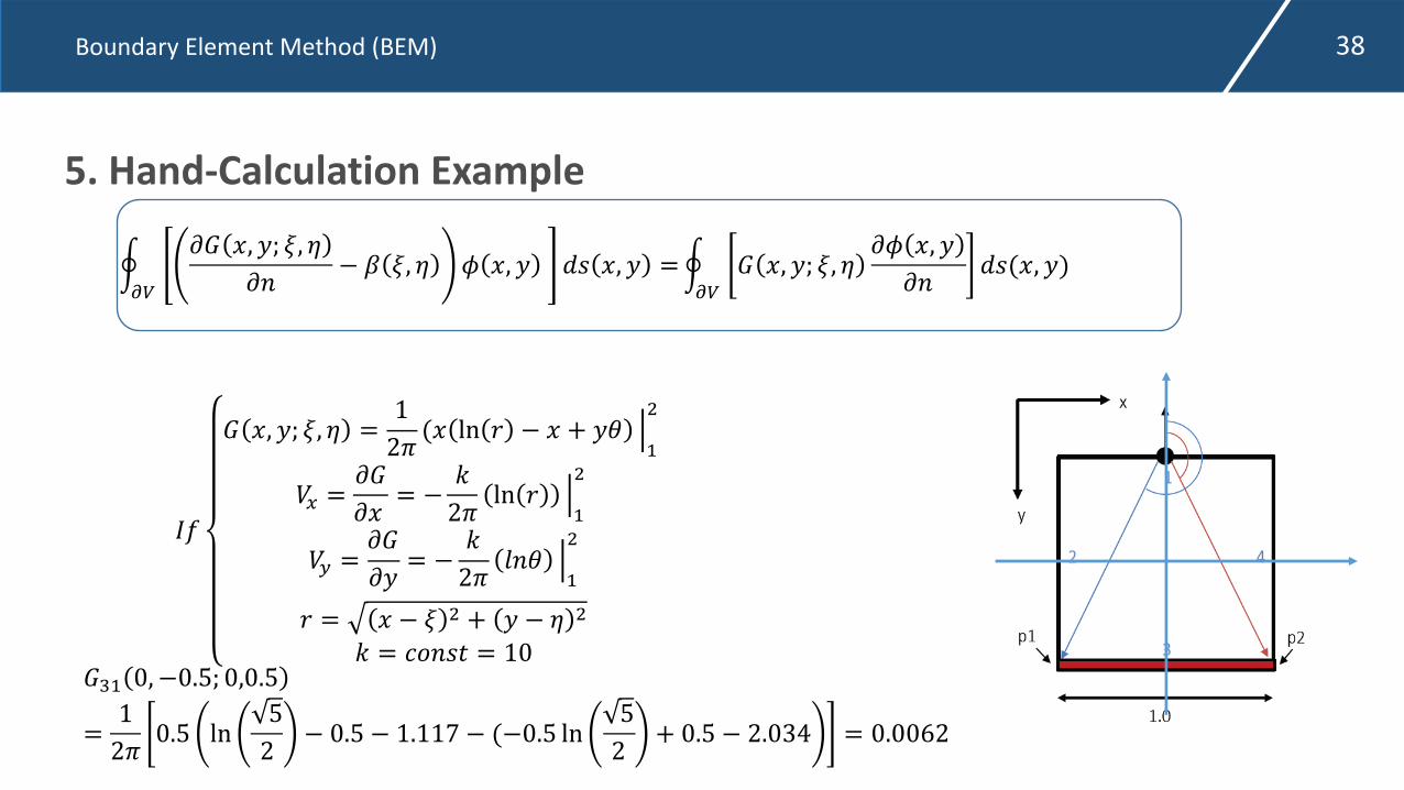
5. Hand-Calculation Example
!"#
$% &, (; *, +$,
− . *, + / &, ( 01 &, ( =!"#
% &, (; *, +$/ &, ($,
01(&, ()
56
% &, (; *, + =129
(& ln < − & + (> ?@
A
BC =$%$&
= −D29
ln < ?@
A
BE =$%$(
= −D29
F,> ?@
A
< = & − * A + ( − + A
D = GH,1I = 10%K@ 0, −0.5; 0,0.5
=129
0.5 ln52
− 0.5 − 1.117 − (−0.5 ln52
+ 0.5 − 2.034 = 0.0062

Boundary Element Method (BEM) 39
5. Hand-Calculation Example
!"#
$% &, (; *, +$,
− . *, + / &, ( 01 &, ( =!"#
% &, (; *, +$/ &, ($,
01(&, ()
56
% &, (; *, + =129
(& ln < − & + (> ?@
A
$%$,
= −B29
ln < ?@
A
< = & − * A + ( − + A
B = CD,1E = 10
%@@ %@A %@G %@H%A@ %AA %AG %AH%G@ %GA %GG %GH%H@ %HA %HG %HH
=
−0.27 −0.053 0.006 −0.053−0.053 −0.27 −0.053 0.0060.006 −0.053 −0.27 −0.053−0.053 0.006 −0.053 −0.27
Boundary Element Method (BEM) 40
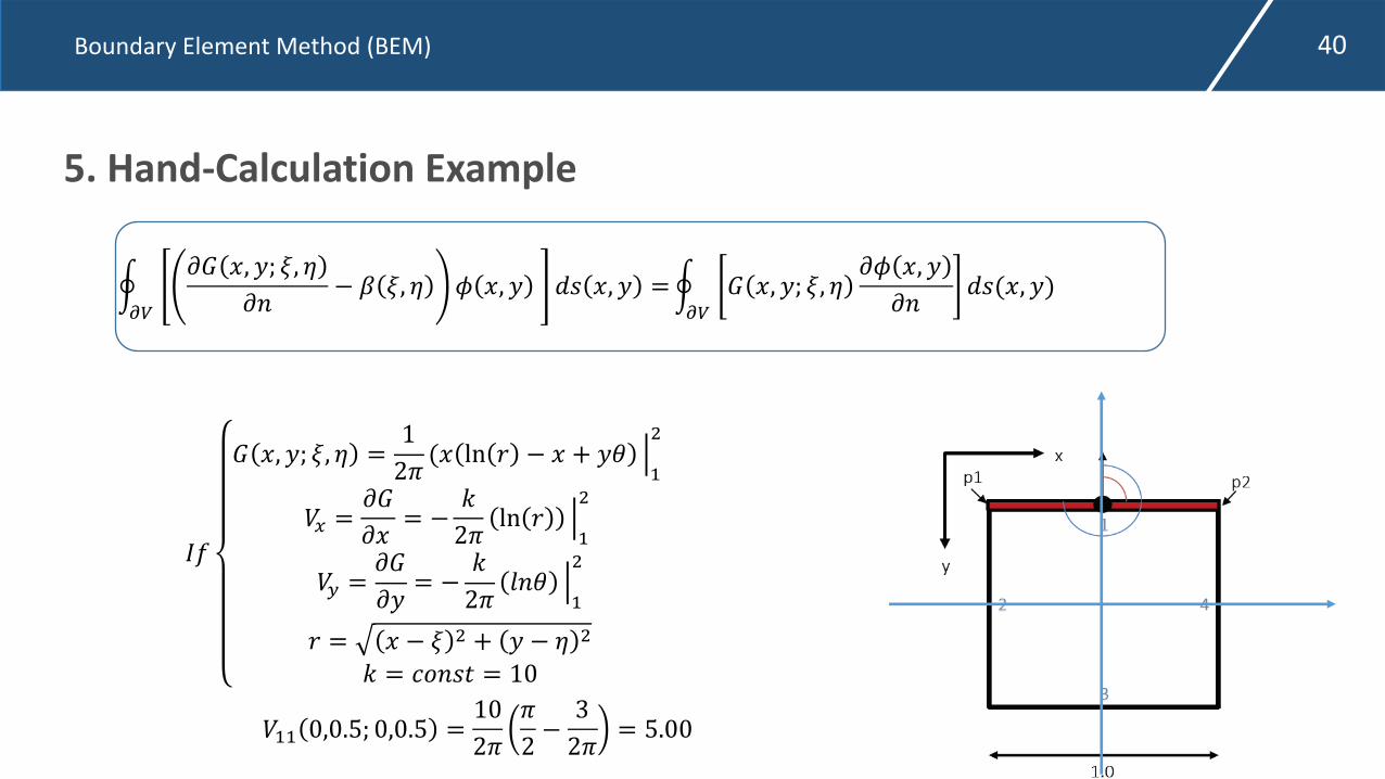
5. Hand-Calculation Example
!"#
$% &, (; *, +
$,− . *, + / &, ( 01 &, ( =!
"#% &, (; *, +
$/ &, (
$,01(&, ()
56
% &, (; *, + =1
29(& ln < − & + (> ?
@
A
BC =$%$&
= −D29
ln < ?@
A
BE =$%
$(= −
D
29F,> ?
@
A
< = & − * A + ( − + A
D = GH,1I = 10
B@@ 0,0.5; 0,0.5 =10
29
9
2−3
29= 5.00

Boundary Element Method (BEM) 41
5. Hand-Calculation Example
!"#
$% &, (; *, +
$,− . *, + / &, ( 01 &, ( =!
"#% &, (; *, +
$/ &, (
$,01(&, ()
56
% &, (; *, + =1
29(& ln < − & + (> ?
@
A
BC =$%
$&= −
D
29ln < ?
@
A
BE =$%
$(= −
D
29F,> ?
@
A
< = & − * A + ( − + A
D = GH,1I = 10
B@A 0, −0.5; 0,0.5 =10
29ln 0.5 − ln
5
2= −1.281
Boundary Element Method (BEM) 42
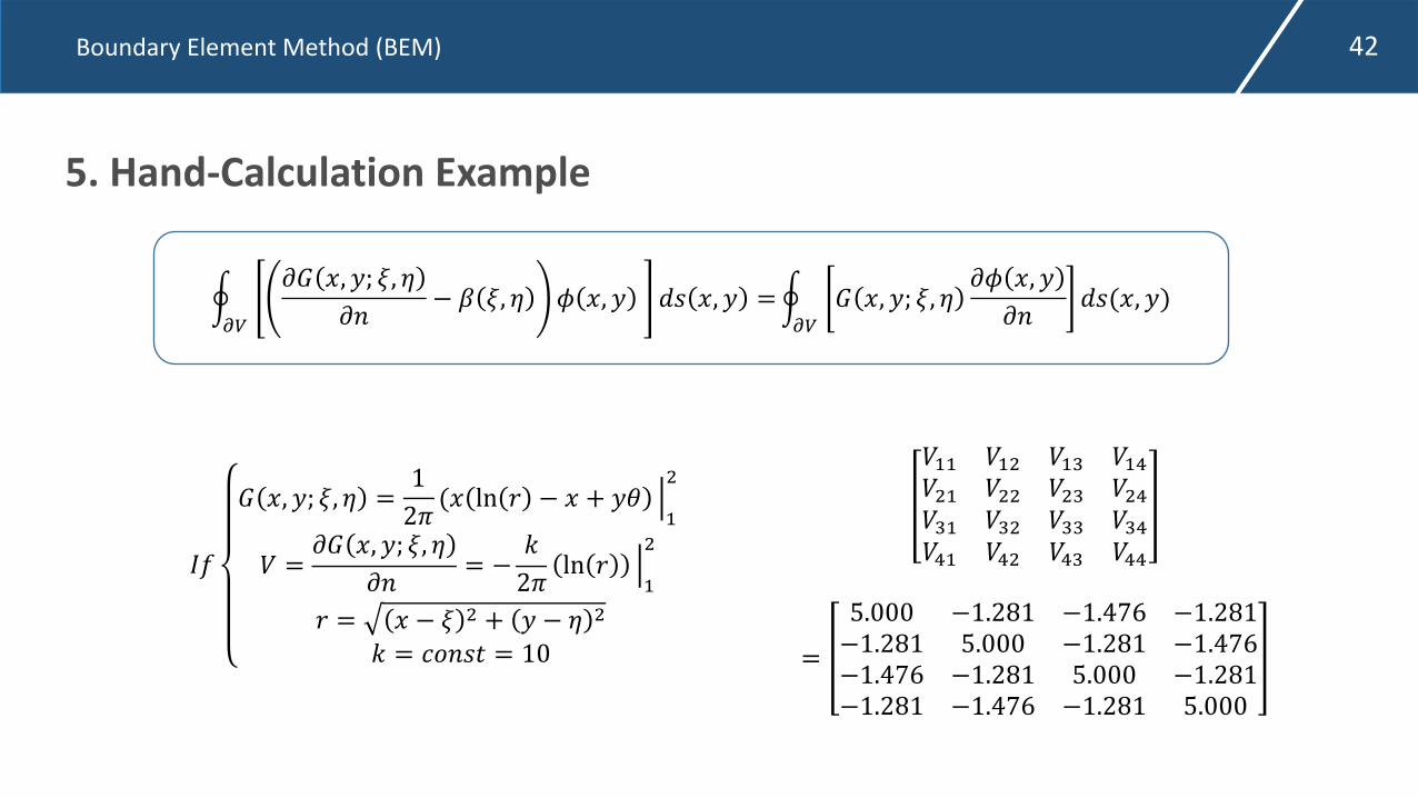
5. Hand-Calculation Example
!"#
$% &, (; *, +$,
− . *, + / &, ( 01 &, ( =!"#
% &, (; *, +$/ &, ($,
01(&, ()
56
% &, (; *, + =129
(& ln < − & + (> ?@
A
B =$% &, (; *, +
$,= −
C29
ln < ?@
A
< = & − * A + ( − + A
C = DE,1F = 10
B@@ B@A B@H B@IBA@ BAA BAH BAIBH@ BHA BHH BHIBI@ BIA BIH BII
=
5.000 −1.281 −1.476 −1.281−1.281 5.000 −1.281 −1.476−1.476 −1.281 5.000 −1.281−1.281 −1.476 −1.281 5.000
Boundary Element Method (BEM) 43
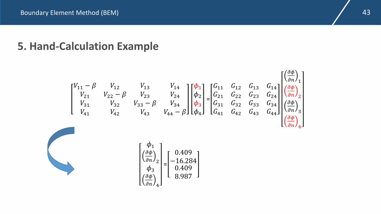
5. Hand-Calculation Example
!"" − $ !"% !"& !"'!%" !%% − $ !%& !%'!&" !&% !&& − $ !&'!'" !'% !'& !'' − $
("(%(&('
=
)"" )"% )"& )"')%" )%% )%& )%')&" )&% )&& )&')'" )'% )'& )''
*+*, "*+*, %*+*, &*+*, '
("*+*, %(&*+*, '
=0.409−16.2840.4098.987
Boundary Element Method (BEM) 44
Contents1. Introduction
2. Historical Perspective
3. General Principles
4. Governing Equations
5. Hand-Calculation Example
6. Numerical Example
7. Example Applications
Boundary Element Method (BEM) 45
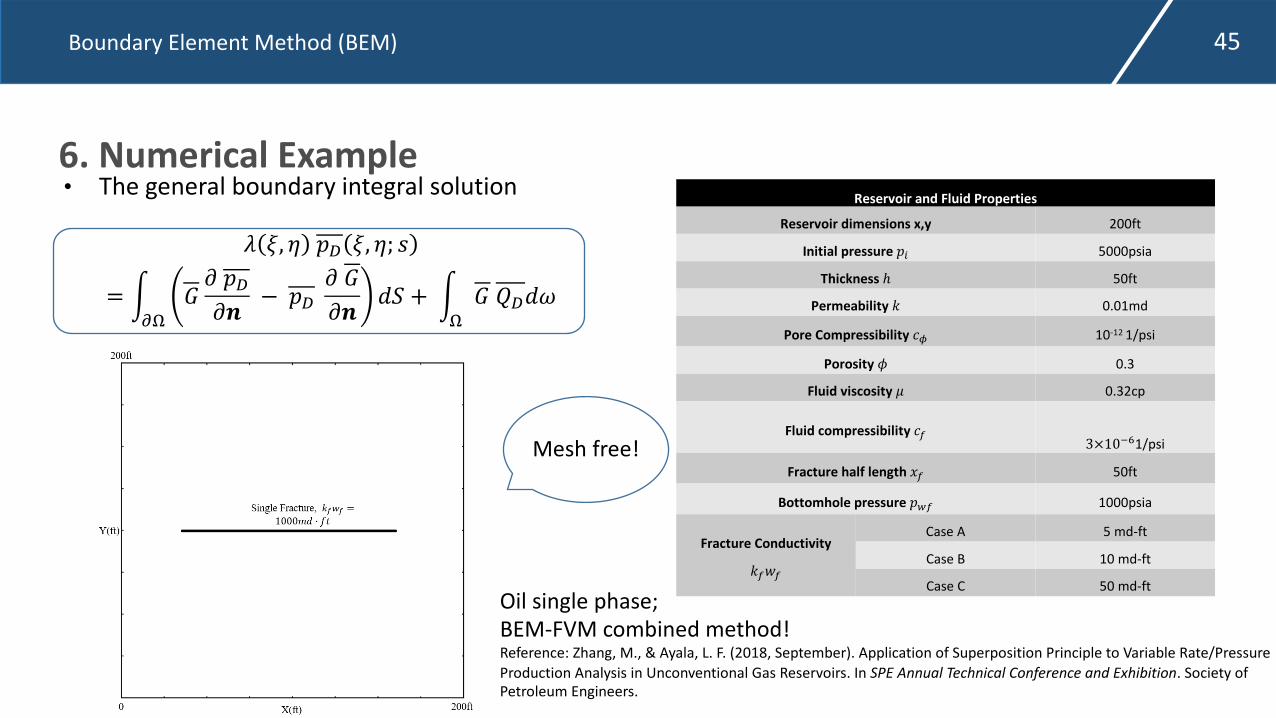
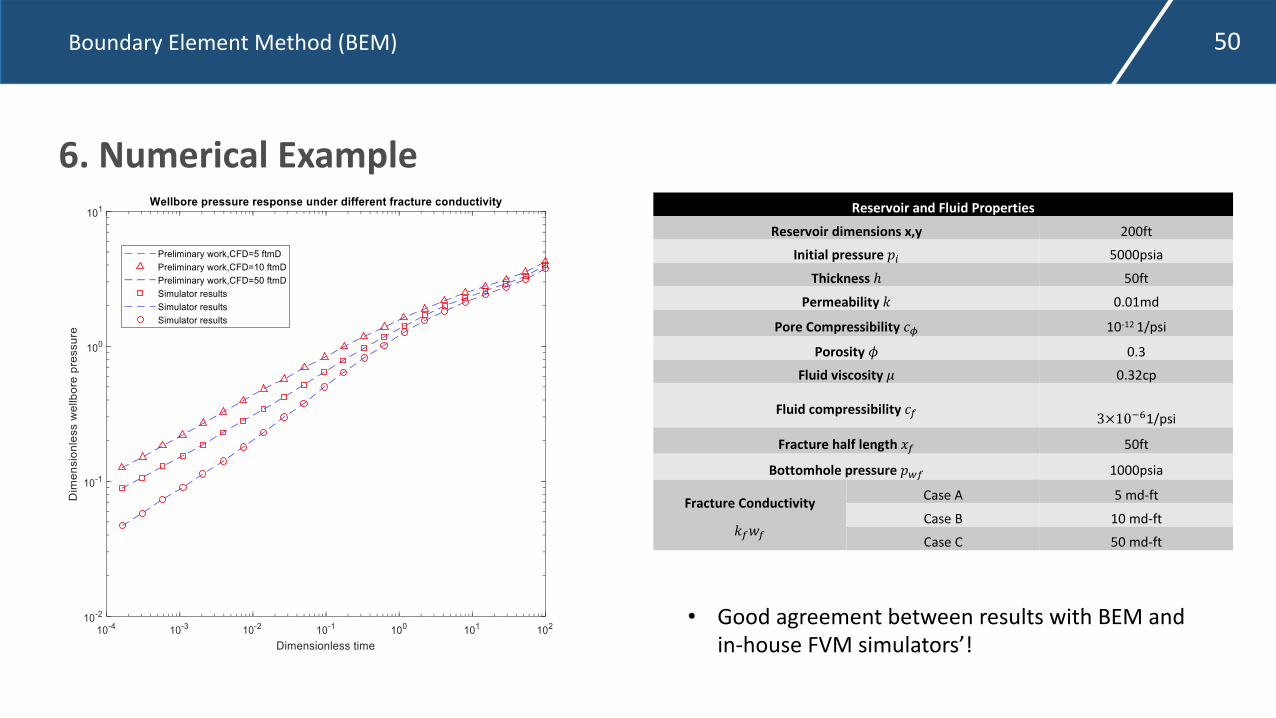
6. Numerical Example• The general boundary integral solution
! ", $ %& ", $; (
= *+,
- . %&./ − %&. -./ 12 + *
,- 4&15
Reservoir and Fluid PropertiesReservoir dimensions x,y 200ft
Initial pressure %6 5000psia
Thickness ℎ 50ft
Permeability 8 0.01md
Pore Compressibility 9: 10-12 1/psi
Porosity ; 0.3
Fluid viscosity < 0.32cp
Fluid compressibility 9= 3×10BC1/psi
Fracture half length D= 50ft
Bottomhole pressure %E= 1000psia
Fracture Conductivity
8=F=
Case A 5 md-ft
Case B 10 md-ft
Case C 50 md-ft
Mesh free!
Oil single phase;BEM-FVM combined method!Reference: Zhang, M., & Ayala, L. F. (2018, September). Application of Superposition Principle to Variable Rate/Pressure Production Analysis in Unconventional Gas Reservoirs. In SPE Annual Technical Conference and Exhibition. Society of Petroleum Engineers.
Boundary Element Method (BEM) 46
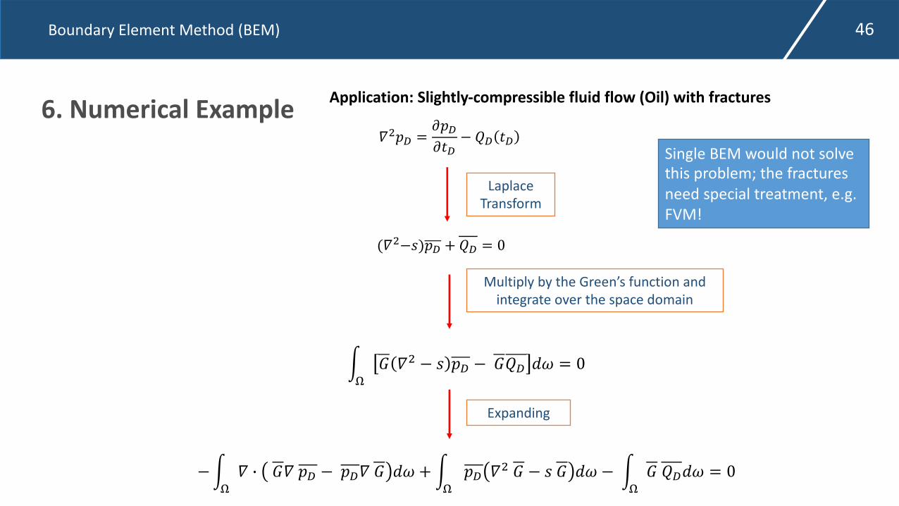
6. Numerical Example Application: Slightly-compressible fluid flow (Oil) with fractures
!"#$ =&#$&'$
− )$ '$
Laplace Transform
(!"−+)#$ + )$ = 0
Multiply by the Green’s function and integrate over the space domain
/0
1 !" − + #$ − 1)$ 23 = 0
−/0! 4 1! #$ − #$! 1 23 +/
0#$ !" 1 − + 1 23 − /
01 )$23 = 0
Expanding
Single BEM would not solve this problem; the fractures need special treatment, e.g. FVM!
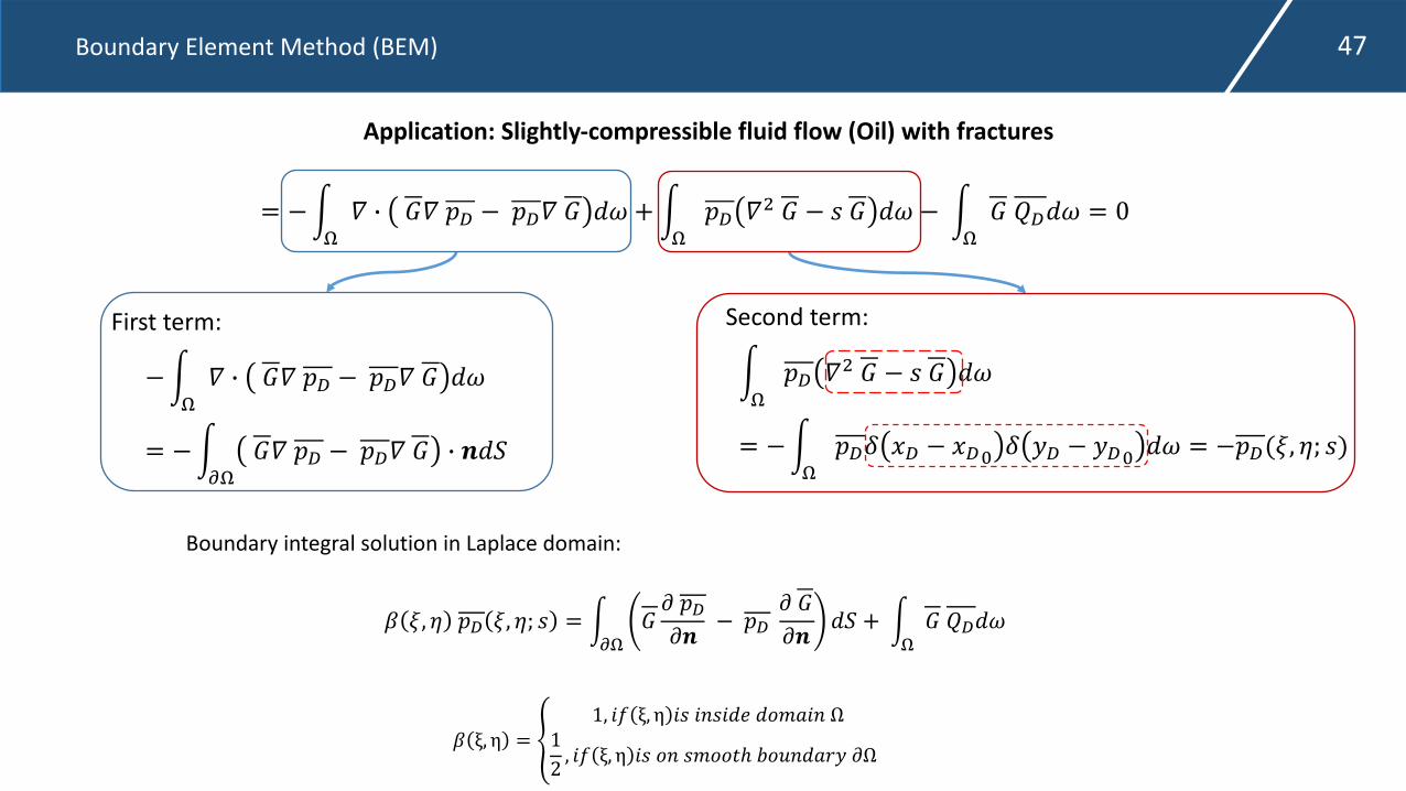
Boundary Element Method (BEM) 47
= −#$% & '% () − ()% ' *+ +#
$() %- ' − . ' *+ − #
$' /)*+ = 0
First term:
−#$% & '% () − ()% ' *+
= −#1$
'% () − ()% ' & 2*3
Second term:
#$() %- ' − . ' *+
= −#$()4 5) − 5)6 4 7) − 7)6 *+ = −()(9, ;; .)
Boundary integral solution in Laplace domain:
> 9, ; () 9, ;; . = #1$
'? ()?2
− ()? '?2
*3 + #$' /)*+
> ξ, η = B1, DE ξ, η D. DF.D*G *HIJDF Ω
12, DE ξ, η D. HF .IHHMℎ OHPF*JQ7 ?Ω
Application: Slightly-compressible fluid flow (Oil) with fractures

Boundary Element Method (BEM) 48
6. Numerical Example
• Efficient and implicit;• No iteration is required!
Flow chart for oil single phase using Boundary Element Method
Boundary Element Method (BEM) 49
6. Numerical Example• The general boundary integral solution
! ", $ %& ", $; (
= *+,
- . %&./ − %&. -./ 12 + *
,- 4&15
Mesh free!
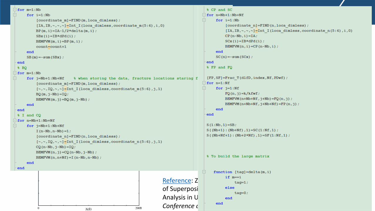
Reference: Zhang, M., & Ayala, L. F. (2018, September). Application of Superposition Principle to Variable Rate/Pressure Production Analysis in Unconventional Gas Reservoirs. In SPE Annual Technical Conference and Exhibition. Society of Petroleum Engineers.
Boundary Element Method (BEM) 50
6. Numerical ExampleReservoir and Fluid Properties
Reservoir dimensions x,y 200ftInitial pressure !" 5000psia
Thickness ℎ 50ftPermeability $ 0.01md
Pore Compressibility %& 10-12 1/psi
Porosity ' 0.3Fluid viscosity ( 0.32cp
Fluid compressibility %) 3×10./1/psi
Fracture half length 0) 50ft
Bottomhole pressure !1) 1000psia
Fracture Conductivity
$)2)
Case A 5 md-ftCase B 10 md-ftCase C 50 md-ft
• Good agreement between results with BEM and in-house FVM simulators’!
Boundary Element Method (BEM) 51
Contents1. Introduction
2. Historical Perspective
3. General Principles
4. Governing Equations
5. Hand-Calculation Example
6. Numerical Example
7. Example Applications
Boundary Element Method (BEM) 52
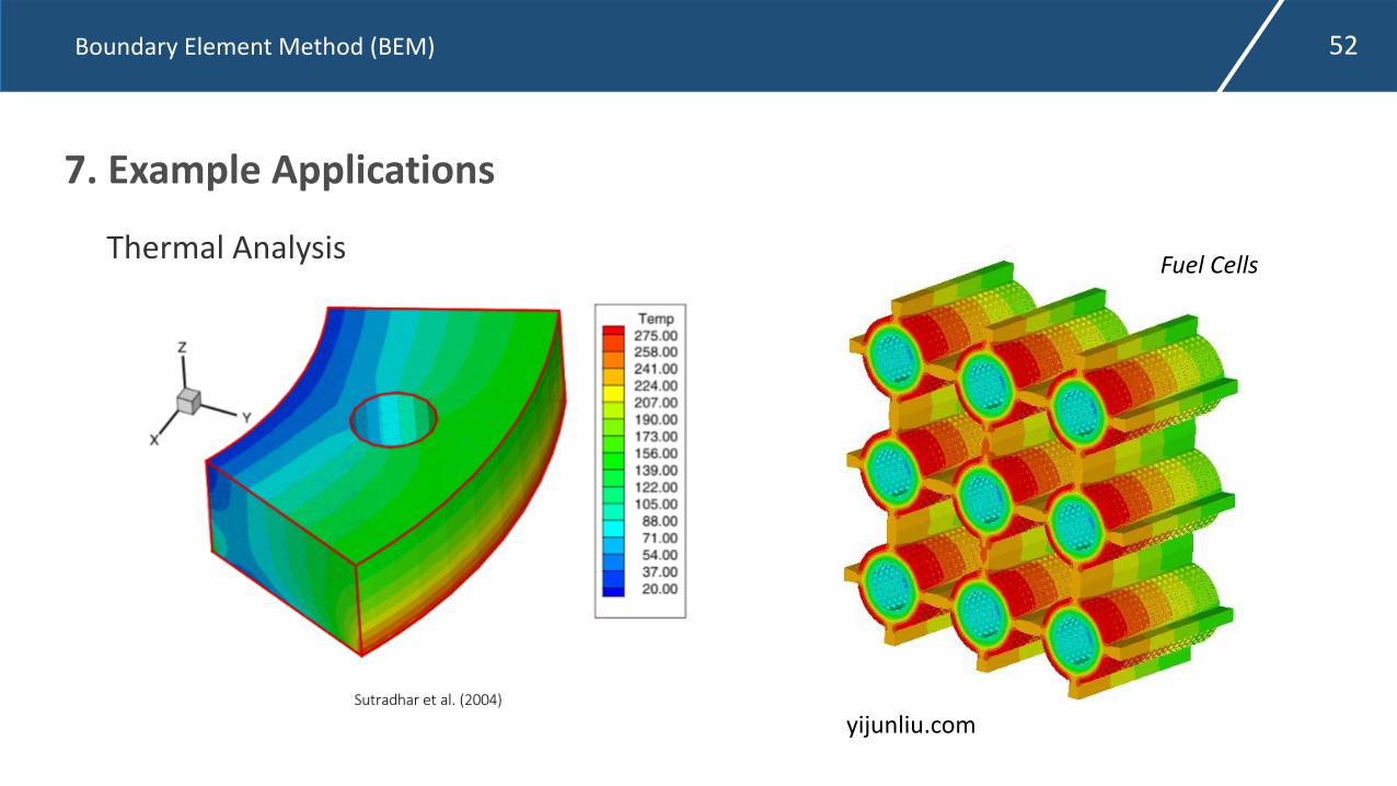
7. Example ApplicationsThermal Analysis Fuel Cells
yijunliu.com
Boundary Element Method (BEM) 53
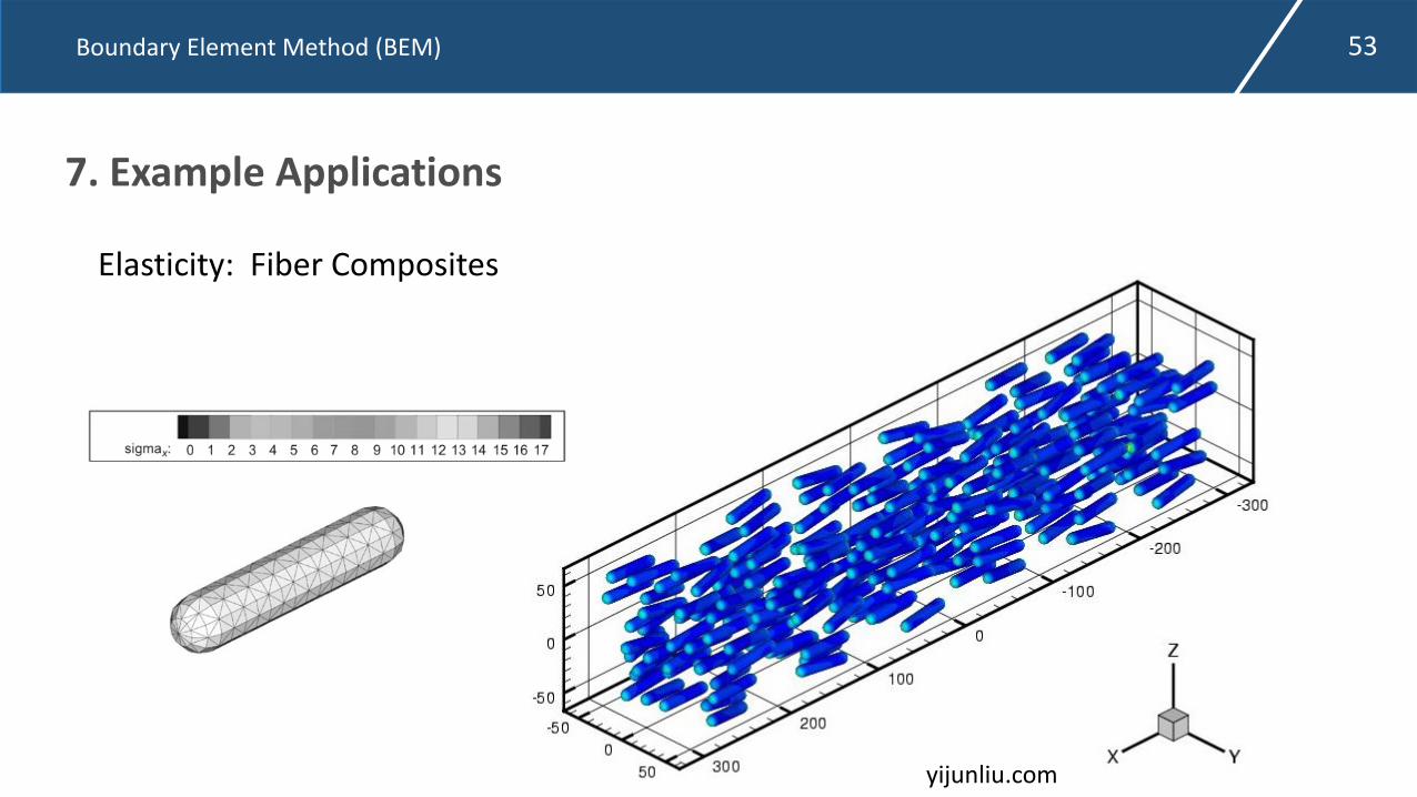
7. Example Applications
Elasticity: Fiber Composites
yijunliu.com
Boundary Element Method (BEM) 54
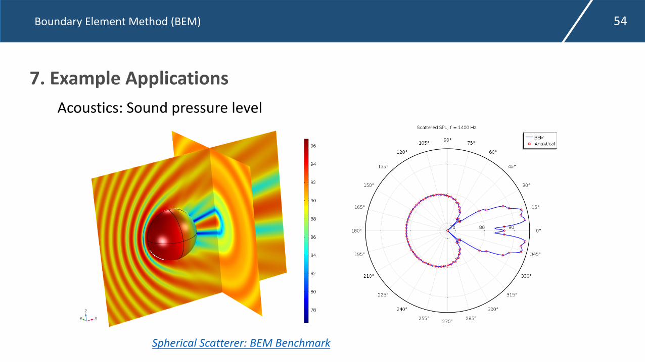
7. Example Applications
Spherical Scatterer: BEM Benchmark
Acoustics: Sound pressure level

Boundary Element Method (BEM) 55
7. Example Applications
Magnetostatics Modeling
comsol.com
Boundary Element Method (BEM) 56
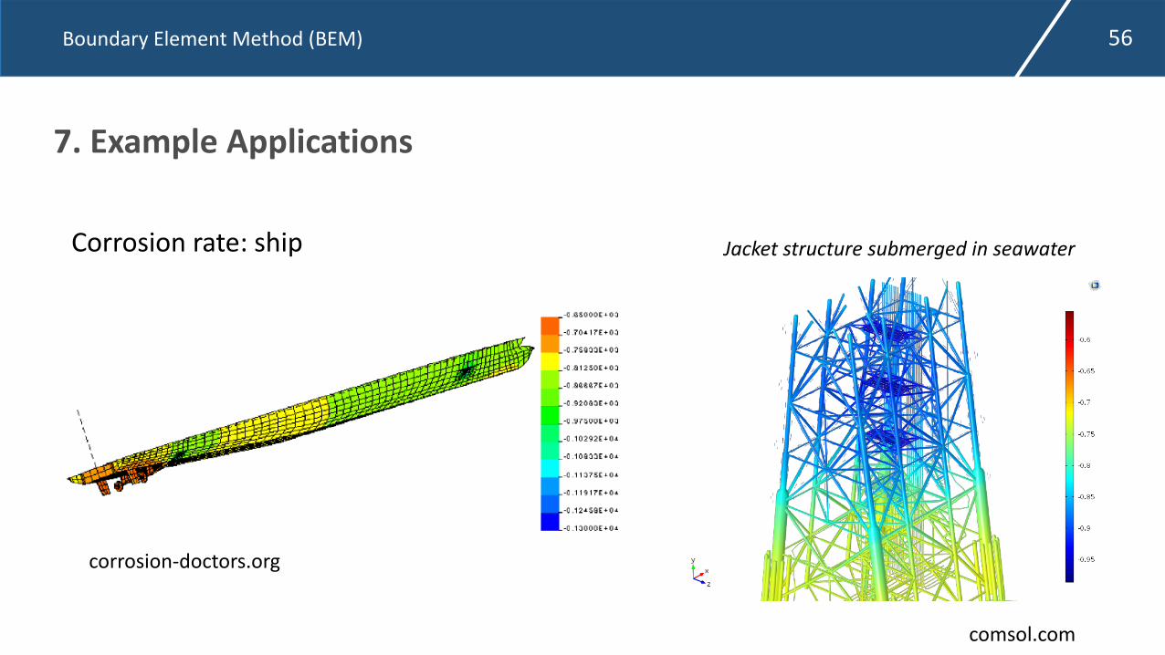
7. Example Applications
corrosion-doctors.org
Corrosion rate: ship
comsol.com
Jacket structure submerged in seawater
References• Fredholm E. I. (1903). Sur une classe d'equations fonctionnelles. Acta Math., 27, 365–390.
• Banerjee P. K. and Butterfield R. (1975), Boundary Element Methods in Geomechanics.
• Brebbia CA. The boundary element method for engineers. London/New York: Pentech Press/HalsteadPress; 1978.
• Gauss C. F. (1813). Theoria attractionis corporum sphaeroidicorum ellipticorum homogeneorum methodonova tractate. Commentationes societatis regiae scientiarium Gottingensis recentiores, 2: 355–378.
• Liu, Y. J., et al. "Recent advances and emerging applications of the boundary element method." AppliedMechanics Reviews 64.3 (2011): 030802.
• Cheng, A. H-D., and Cheng D. T. (2005). Heritage and early history of the boundary element method.Engineering Analysis with Boundary Elements 29.3: 268-302.
• Green G. An essay on the application of mathematical analysis to the theories of electricity andmagnetism. Printed for the Author by Wheelhouse T. Nottigham; 1828. 72 p. Also, Mathematical papersof George Green. Chelsea Publishing Co.; 1970. p. 1–115.
Boundary Element Method (BEM) 57

References• Pecher, R., & Stanislav, J. F. (1997). Boundary element techniques in petroleum reservoir simulation.
Journal of Petroleum Science and Engineering, 17(3-4), 353-366.
• Couran, R., & Hilbert. D. (1953). Methods of Mathematical Physics. 2, Wiley (Interscience), New York, 1stEnglish ed., 830.
• Volterra, V. (2005). Theory of functionals and of integral and integro-differential equations. CourierCorporation.
• Liggett, J. A., & Liu, P. L. F. (1983). The boundary integral equation method for porous media flow. AppliedOcean Research, 5(2), 255.
• Kikani, J., & Horne, R. (1989). Application of boundary element method to reservoir engineering problems.Journal of Petroleum Science and Engineering, 3(3), 229-241.
• Pecher, R. (1999). Boundary element simulation of petroleum reservoirs with hydraulically fractured wells.(Doctoral dissertation, University of Calgary).
• Cruse TA, Rizzo FJ. A direct formulation and numerical solution of the general transient elastodynamicproblem—I. J Math Anal Appl 1968;22:244–59.
Boundary Element Method (BEM) 58

References• Fang, S., Cheng, L., & Ayala, L. F. (2017). A coupled boundary element and finite element method for the
analysis of flow through fractured porous media. Journal of Petroleum Science and Engineering, 152, 375-390.
• Zhang, M., & Ayala, L. F. (2018). A General Boundary Integral Solution for Fluid Flow Analysis in Reservoirswith Complex Fracture Geometries. Journal of Energy Resources Technology, 140(5), 052907.
• Ang, W. T. (2007). A beginner's course in boundary element methods. Universal-Publishers.
• Cruse TA. The transient problem in classical elastodynamics solved by integral equations. Doctoraldissertation. University of Washington; 1967, 117 pp.
• Jaswon MA, Ponter AR. An integral equation solution of the torsion problem. Proc R Soc, A 1963;273:237–46.
• Beer, Gernot & Smith, Ian & Duenser, Christian. (2008). The Boundary Element Method withProgramming: For Engineers and Scientists. 10.1007/978-3-211-71576-5.
• Trefftz, E. (1926) Ein Gegenstück zum Ritz’schen Verfahren. Proc. 2nd int. Congress in Applied Mechanics,Zurich, pp 131.
Boundary Element Method (BEM) 59
References• Fedele, Francesco, et al. "Fluorescence photon migration by the boundary element method." Journal of
computational physics 210.1 (2005): 109-132.
• http://yijunliu.com/• https://www.comsol.com/model/spherical-scatterer-bem-benchmark-56141
• https://www.comsol.com/• http://corrosion-doctors.org/
Boundary Element Method (BEM) 60
Top Related