


Languages
Pages
Legal


1
Cultural Resource Management and GIS
A Course Project
Written by
Marikka Williams
For Geog 5550 – Advanced GIS
Instructor: Dr. Minhe Ji
Fall 2002
2
Introduction
It is the professional responsibility of the cultural resource manager to direct
archaeological efforts in areas defined by political boundaries. In addition, it is the ethical
responsibility of an archaeologist to analyze and publish accurate data concerning ancient
inhabitants who occupied the landscape. As a result, it is important that site formation
processes are not only understood but also evaluated so that accurate, chronological
information can be extracted. With the help of GIS, cultural resource managers can work
closely with archaeologists and direct excavation efforts to well preserved archaeological sites
that are threatened by development. Cultural resource managers and city planners have the
daunting task of protecting archaeological remains in the midst of rapid population growth and
development. There are several laws that protect archaeological resources yet with at least
12,000 years of human occupation in North America it is difficult to know precisely where to
begin. To a certain extent sites of proposed development are surveyed but this process is
lengthy, arduous and often randomly conducted. Implementation of a GIS model would help
pinpoint specific areas for detecting “in situ” sites and/or “high risk” areas in order to promote
preservation, excavation and analysis in a more efficient manner.
Site Formation Processes
Archaeologists excavate archaeological remains for the purpose of extracting
information in order to reconstruct the past and develop theories that explain ancient behaviors.
With this objective in mind it is crucial to consider the accuracy of the data from which these
theories are being built upon. A multitude of techniques have been developed through time in
order to extract as much information as possible from archaeological sites. Unfortunately site
formation processes can create an obscured picture that may lead to the development of
erroneous theories. Wood and Johnson (1978: 315-316) point out that archaeologists have
often operated under the assumption that past human activities are “reflected” (Childe, 1956: 1)
and even “fossilized” (Binford, 1964: 424) in the “highly patterned” distribution of “all”
3
archaeological remains (Thompson and Longacre, 1966: 270). By 1968, archaeologists such
as Ascher, followed by Krause and Thorne in 1971, and Schiffer in 1972 began to shift attention
to the effects of site formation processes on the archaeological record. Over the past 30 years
a tremendous amount of literature has been dedicated to the study of site formation processes.
To my knowledge there is not any literature that addresses predicting site disturbance prior to
excavation for the purposes of cultural resource management in the context of salvage
archaeology. Furthermore, as of yet, no GIS applications address site formation processes and
potential for disturbance once the site has been excavated. If site formation processes can be
identified prior to excavation it will save a lot of time and lead to greater accuracy in the
archaeological record.
Predicting "Archaeological Sensitive" Areas
Predictive models have been widely criticized in the archaeological community. Ebert
(2000) argues that inductive predictive modelling methods are inefficient in terms of detecting a
lack of homogeneity in one's data and criticizes the translation of maps into variables. He
claims that it focuses on sites rather than systems and attempts to relate location to
environmental variables do not have a "theoretical basis" to be effective predictors. According
to Warren and Asch (2000: 6) most archaeological predictive models rest the assumptions that
settlement choices made by ancient people were strongly influenced by characteristics of the
natural environment and that these factors are accurately depicted on modern maps. Woodman
and Woodword have noted that "case control" studies are often used in predictive modelling.
Procedures such as logistic regression assume a linear relationship between dependent and
independent variables, which can take the form of correlation, confounding or interaction. In
one case study 46 known prehistoric sites in an area, known as the Aberdeen Proving Ground
(APG), helped facilitate an effective way to locate the variable potential of other archaeological
sites in the area. The investigators decided to study a database containing 572 prehistoric sites
located in areas of Upper Chesapeake Bay (UCB) that most closely resembled the environment

4
of the APG. The researchers utilized a deductive approach and divided the sites from the UCB
into shell midden and lithic scatter categories. Their basic assumption was that the different
sites would be located in different circumstances with respect to soil, soil drainage, proximity to
water, topographic setting, slope and aspect. These characteristics were recorded from the
UCB database along with a comparative background sample of 500 random locations taken
from within the APG. To decide which variables to use in the construction of their specific
predictive model the authors utilized an inductive procedure based upon the generation of a
series of frequency tables for the site and random background locations with respect to each of
the environmental variables and combinations of variables. This enabled them to eliminate the
variables that were not relative to site prediction. They narrowed their variables down to
proximity to water, water type, elevation range, and topographic setting. The authors chose to
create weightings for particular combinations of classes possible between the four predictors.
Construction of the predictive model involved combining the four variables and allocating each
cell its appropriate potential classification dependent upon the unique combination of variables.
The accuracy of the model was initially evaluated by comparing the known 46 prehistoric site
locations within the APG to it. A more formal assessment of the overall performance of this
model was performed by calculating Kvamme's simple gain statistic: Gain=1-(% of total area
covered by model % of total sites within model area). This is based on the assumption that if the
high potential area is small relative to the overall study area and the number of sites found
within it is large in relation to the total for the entire study area then it is a fairly good model
(Kvamme 1988: 329). This is only one example of the many case studies that have been
conducted to construct archaeological site prediction models.
Research Goals
Geographic Information System Software has been utilized in a variety of archaeological
studies. Most of the data that archaeologists recover is spatial in character. As a result, GIS
has excellent potential for analyses, planning, and management of archaeological resources.
5
For the purposes of this research paper I focused on the organization or archaeological data,
prediction of sites and planning for cultural resource management survey. First I will organize
and integrate spatial and descriptive archaeological information into a geodatabase. Then, I
will utilize GIS to determine where to survey and maximize recovery or protection of “in situ”
archaeological sites. In addition, I make an effort to explain the location of sites and their
relative preservation. My ultimate goal is to apply GIS as a mechanism to create a series of
analytical archaeological resource maps that will facilitate efficient and effective cultural
resource management, planning, mitigation, preservation, excavation and analysis.
Methodology
The purpose of this research is to build a GIS model that will organize previously
documented archaeological information, predict probable archaeological site locales, explain
known site locations, evaluate relative site formation processes and select areas for
archaeological survey. As a result, this project consists of a research design that encompasses
calculating the revised universal soil loss equation, computing cost weighted distance, least cost
pathways, and overlay analysis. These facets are analyzed individually and then juxtaposed in
order to maximize data retrieval. First, the revised universal soil loss equation is calculated in
ArcView 8.0 Spatial Analyst ‘Raster Calculator’ to determine the potential for soil erosion and
located areas of increased sedimentation. Next, least cost pathways based on weighted
distance and shortest paths were also calculated in the Spatial Analyst Extension to establish
“archaeologically sensitive” areas. The shortest paths that were calculated between three
source sites and a sample of 150 other sites were given a buffer of 100 meters. These
pathways were then clipped based on the city and lake boundaries to provide more detail.
Finally, an ‘Overlay Analysis’ facilitated by the ‘Geo-Processing Tools’ in ArcView 8.0 was
conducted in order to make the final selection of three site areas that would be suitable
locations for archaeological survey. The Conceptual Diagram illustrated in Figure 1 provides a
view of the general initial process required to achieve these goals.

6
Cultural Resource Management Plan
Figure 1. Conceptual Diagram of Goals, Data Layers and Methods
Data Layer Management
Data layers required for this case study included archaeological spatial coordinates,
Digital Elevation Model (DEM) files, soils, vegetation, landuse, roads, lakes, streams, city, and
county boundaries. I acquired my base data layers or base information from ESRI, TNRIS,
North Central Texas Council of Governments, and the Texas Archaeological Resource
Laboratory in Austin. The archaeological data required conversion from excel .dbf files to shape
files. It was necessary to define the projection parameters for all of the data layers and then
Archaeology
Slope
Roads
Lakes
Streams
Soils
Vegetation
City Boundaries
County Boundaries Site Preservation
Sinks
Site Prediction
Shortest Path
Site Selection
OVERLAY ANALYSIS
Cost Weighted Distance
Potential for Habitat
RUSLE Values
DEM Cultural Resource Managment
Land Use

7
project the all of the data layers to the same coordinate system. I chose UTM NAD 1927 Zone
14N to match the coordinate origination of the archaeological sites. The procedure that I
followed to manage the data layers required the following steps:
?? Data acquisition: ESRI, TNRIS, DFWINFO, TARL ?? Conversion from database files to shape files. ?? Defining projection parameters for all data layers. ?? Projection of all data layers to same coordinate system (UTM NAD 1927 Zone 14N). ?? Creation of Geo-databases to manage data analysis.
The final step prior to analysis was to create a Geodatabase to manage the volume of
data collected during this study. Figure 2 illustrates the Geodatabase design that I constructed.
I created a Personal Geodatabase with Feature Datasets that contained numerous Feature
Classes as you can see here. The only data layers that I could not include in my Geodatabase
were the raster files that I had to file in folders separately.
Figure 2. Geodatabase Design
8
Study Area
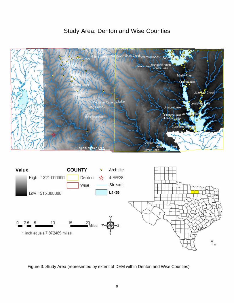
Denton and Wise Counties, situated in North Texas, are ideal settings for conducting
archaeological research of this nature. These areas encompass two major environmental
zones, the Western Cross Timbers and the Grand Prairie. The sites in Wise County are located
primarily in pastures near minor tributaries whereas the sites in Denton County were situated
near the Trinity River before the impoundment of Lewisville Lake. The parameters of the study
area established in these counties are expressed by the DEM in figure 3. The location of the
Lewisville Lake sites are beneficial with respect to providing information to cultural resource
managers that is related to the effects of reservoirs on peripheral sites. Knowing the potential
for future site disturbance is important for cultural resource management purposes. Being
aware of past site formation processes is pertinent in terms of the accuracy of archaeological
excavations and benefits both fields. Site Catchment areas will be developed based on the
location of specific test units within known sites in Wise and Denton Counties. These known
sites will provide specific variables that will establish the specific character of the
microenvironment of each area. Following excavation, and prior to intensive archaeological
analysis, it should be first determined which specific test units have been disturbed and which
specific units are chronologically stratified. Beyond detecting mere presence of site
disturbance, it is necessary to ascertain the degree of disturbance in certain locations so that
further excavation can be directed to locations that are more likely to be undisturbed. These “in
situ” areas will provide accurate, meaningful data that has the capacity to contribute to the
archaeological record. Once the “in situ” units or areas are pinpointed, the general character of
occupations (who they were, when they lived, what they did) can be determined, relative cultural
ecological systems (how they related to the landscape) examined, and variables surrounding
specific site location evaluated. Based on comparative data between sites, the validity of a GIS
model, built to predict and explain the location of “in situ” versus disturbed sites, will be tested
with other known site locations or in the field.
9
Study Area: Denton and Wise Counties
Figure 3. Study Area (represented by extent of DEM within Denton and Wise Counties)
10
Differential Preservation: Revised Universal Soil Loss Equation
Calculation of RUSLE is incorporated in order estimate past and future erosion potential
at the archaeological site locations. It is also utilized as a mechanism to pinpoint areas that are
susceptible to erosion or sedimentation. In order to get a handle on relative Site preservation I
calculated the Revised Universal Soil Loss Equation on the study area with intentions to:
?? Identify areas susceptible to erosion. ?? Identify areas receiving sedimentation. ?? Evaluate how these areas correspond with existing archaeology. ?? Seek explanations for disturbed versus stratified sites and try to establish areas that
have the appropriate conditions for stratification. ?? Prioritize Cultural Resource Mitigation.
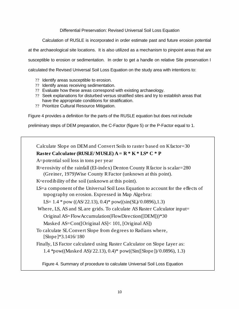
Figure 4 provides a definition for the parts of the RUSLE equation but does not include
preliminary steps of DEM preparation, the C-Factor (figure 5) or the P-Factor equal to 1.
Figure 4. Summary of procedure to calculate Universal Soil Loss Equation
Calculate Slope on DEM and Convert Soils to raster based on K factor=30Raster Calculator (RUSLE/MUSLE) A = R * K * LS* C * PA=potential soil loss in tons per yearR=erosivity of the rainfall (EI-index) Denton County R factor is scalar=280
(Greiner, 1979)Wise County R Factor (unknown at this point).K=erodibility of the soil (unknown at this point).LS=a component of the Universal Soil Loss Equation to account for the effects of
topography on erosion. Expressed in Map Algebra:LS= 1.4 * pow ((AS/22.13), 0.4)* pow((sin(SL)/0.0896),1.3)
Where, LS, AS and SL are grids. To calculate AS Raster Calculator input=Original AS=FlowAccumulation(FlowDirection([DEM]))*30Masked AS=Con([Original AS]< 101, [Original AS])
To calculate SL Convert Slope from degrees to Radians where, [Slope]*3.1416/180
Finally, LS Factor calculated using Raster Calculator on Slope Layer as:1.4 *pow((Masked AS)/22.13), 0.4)* pow((Sin([Slope])/0.0896), 1.3)
11
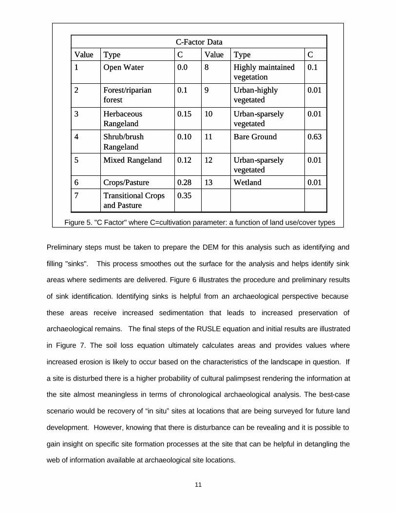
Figure 5. "C Factor" where C=cultivation parameter: a function of land use/cover types
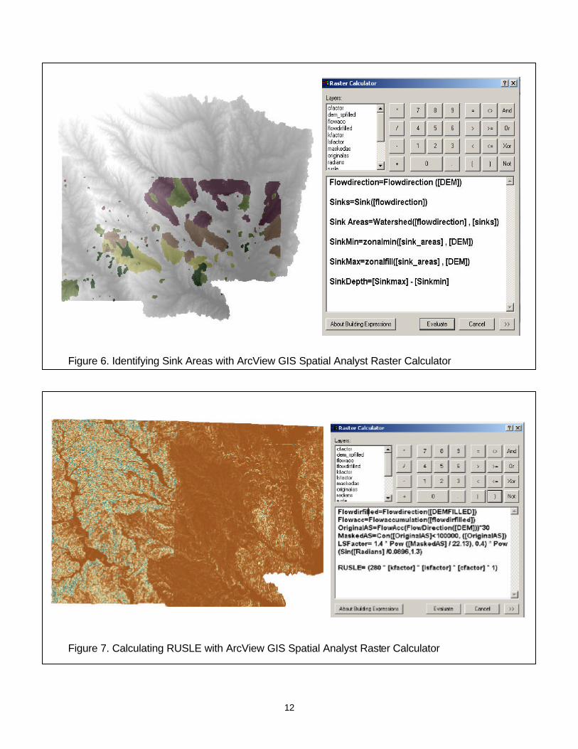
Preliminary steps must be taken to prepare the DEM for this analysis such as identifying and
filling "sinks". This process smoothes out the surface for the analysis and helps identify sink
areas where sediments are delivered. Figure 6 illustrates the procedure and preliminary results
of sink identification. Identifying sinks is helpful from an archaeological perspective because
these areas receive increased sedimentation that leads to increased preservation of
archaeological remains. The final steps of the RUSLE equation and initial results are illustrated
in Figure 7. The soil loss equation ultimately calculates areas and provides values where
increased erosion is likely to occur based on the characteristics of the landscape in question. If
a site is disturbed there is a higher probability of cultural palimpsest rendering the information at
the site almost meaningless in terms of chronological archaeological analysis. The best-case
scenario would be recovery of “in situ” sites at locations that are being surveyed for future land
development. However, knowing that there is disturbance can be revealing and it is possible to
gain insight on specific site formation processes at the site that can be helpful in detangling the
web of information available at archaeological site locations.
0.35Transitional Crops and Pasture
7
0.01Wetland130.28Crops/Pasture6
0.01Urban-sparsely vegetated
120.12Mixed Rangeland5
0.63Bare Ground110.10Shrub/brush Rangeland
4
0.01Urban-sparsely vegetated
100.15Herbaceous Rangeland
3
0.01Urban-highly vegetated
90.1Forest/riparian forest
2
0.1Highly maintained vegetation
80.0Open Water1
C Type ValueC Type Value
C-Factor Data
12
Figure 6. Identifying Sink Areas with ArcView GIS Spatial Analyst Raster Calculator
Figure 7. Calculating RUSLE with ArcView GIS Spatial Analyst Raster Calculator

13
Calculating the soil loss equation and projecting the archaeological sites allowed for several
additional observations beyond what I had initially anticipated. In order to get a clear picture of
what is going on it is necessary to look at the interaction of the Archaeology and the landscape
from several different perspectives. Figure 8 shows all of the sites in relation to relative soil
loss. At this scale and resolution it is difficult to see precisely what is happening between the
sites and the areas that demonstrate increased erosion values.
Figure 8. Wise and Denton County Archaeological Sites, Streams, and Soil Loss
When the sites are considered in relation to soil erosion, with regard to the specific time
period, it is possible to get more of a feel of where certain time periods are located in respect to
areas of increased erosion. However, I feel that this sample is biased for a couple of reasons.
First, alot of contract work has been done in Denton County and there are over 500
14
archaeological sites. As a result, the only historical sites that are represented in Denton County
were a component of a site that contained more than one time period. Wise County on the
other hand contains only 57 recorded sites and most of these sites are. There are several sites
that have yet to be reported to TARL but it is an interesting question especially in light of the
increased soil erosion in Wise County as to why there are not as many sites. One factor could
be the lack of reservoir construction but there are also plenty of amateur archaeologists and
private landowners who have uncovered archeological remains. It is possible to conclude that
there is a correlation between soil erosion and site presence due to the much steeper slopes in
Wise County but other factors should be kept in mind as well.
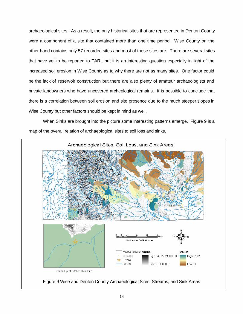
When Sinks are brought into the picture some interesting patterns emerge. Figure 9 is a
map of the overall relation of archaeological sites to soil loss and sinks.
Figure 9 Wise and Denton County Archaeological Sites, Streams, and Sink Areas
15
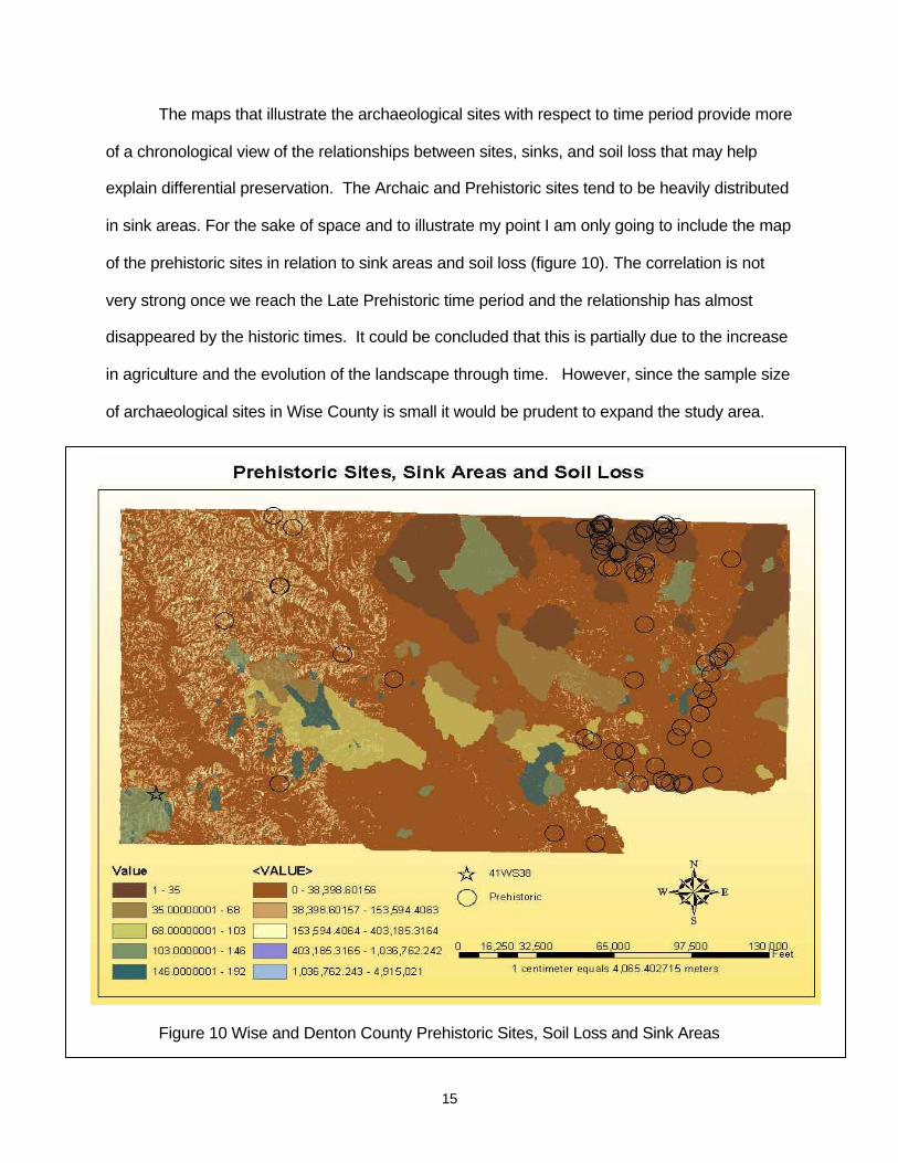
The maps that illustrate the archaeological sites with respect to time period provide more
of a chronological view of the relationships between sites, sinks, and soil loss that may help
explain differential preservation. The Archaic and Prehistoric sites tend to be heavily distributed
in sink areas. For the sake of space and to illustrate my point I am only going to include the map
of the prehistoric sites in relation to sink areas and soil loss (figure 10). The correlation is not
very strong once we reach the Late Prehistoric time period and the relationship has almost
disappeared by the historic times. It could be concluded that this is partially due to the increase
in agriculture and the evolution of the landscape through time. However, since the sample size
of archaeological sites in Wise County is small it would be prudent to expand the study area.
Figure 10 Wise and Denton County Prehistoric Sites, Soil Loss and Sink Areas
16
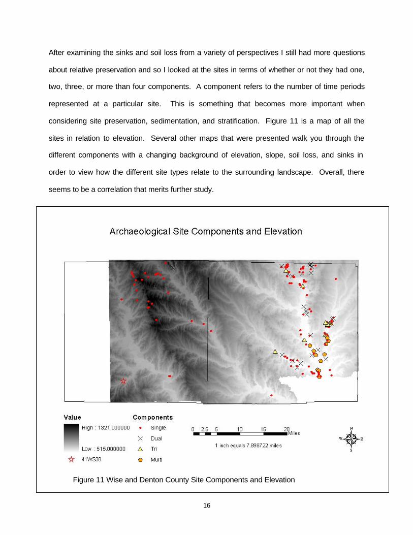
After examining the sinks and soil loss from a variety of perspectives I still had more questions
about relative preservation and so I looked at the sites in terms of whether or not they had one,
two, three, or more than four components. A component refers to the number of time periods
represented at a particular site. This is something that becomes more important when
considering site preservation, sedimentation, and stratification. Figure 11 is a map of all the
sites in relation to elevation. Several other maps that were presented walk you through the
different components with a changing background of elevation, slope, soil loss, and sinks in
order to view how the different site types relate to the surrounding landscape. Overall, there
seems to be a correlation that merits further study.
Figure 11 Wise and Denton County Site Components and Elevation
17
It is clear that soil erosion is more pronounced in the western part of the study area due
to steeper slopes related to deeper stream incision. There appears to be a correlation between
site age, erosion values, and sink presence. It will require further study to determine if there is a
correlation between “in situ” sites and sink presence. Erosion in the western part of the study
area may contribute to the scarcity of sites but it also could be attributed to bias in the record.
As a result of this analysis I feel encouraged to do further study. Elevation, slope, sinks and soil
loss are all important variables that factor into the site formation processes equation. When the
site component facet enters the equation more information emerges. For future studies, with
the perspective of aspect the sites should be looked at on a micro-scale to evaluate site
formation processes on a site level. Also, the study area should be expanded to view a larger
sample size and provide a larger variety to select good case study locales.
Site Prediction
The site prediction model formulated for this case study is based on methods utilized in
the past by other archaeologists, with a few additions, that will fulfill the research goals of this
project. Several articles have been written regarding location models and prediction in the
discovery of archaeological resources. Based on previous case studies, as well as, assumed
relationships between humans and their surrounding eco-system that have been formulated on
the basis of the contents found at local archaeological sites, several core environmental factors
can be employed as variables. However, for the purposes of this study I chiefly considered
slope and soil potential for openland and rangeland habitat to develop least cost pathways
between sites that represented similar time periods or contained similar artifacts.
The central goal of this part of the analysis is to recreate probable “Least Cost” Pathways
that establish parameters to predict “Archaeological Sensitive Areas” and meet the following
conditions:
?? Pathways that would have been most advantageous for ancient humans. ?? Pathways between contemporaneous sites. ?? Pathways between sites containing similar artifacts.
18
GIS has the ability to generate cost surfaces. These surfaces take into consideration not only
proximity or natural resources to the site but also the character of the terrain over which the
proximity is measured. In order to build ‘cost surfaces’, obstructions, barriers, and differences in
the quality of space that may have influenced transportation costs or even perception of the
landscape have been evaluated in other investigations. In this case study ‘cost surface’ is
calculated, based on slope and potential for soils to support vegetation that sustains openland
or rangeland habitat. I chose to use soil potential for two types of habitat based on the types of
animals that were present during prehistoric times and the lack of agriculture. I opted for soils
that have the potential to produce vegetation and suitable habitat for rangeland wildlife and
openland wildlife. These areas would have provided high calorie food for human and animal
population in prehistoric times. The soil data was extracted from the Wise County Soil Survey.
Four categories: high, medium, low, and very low were utilized by soil scientists to classify the
potential for specific soils to support vegetation, that would sustain specific wildlife in the study
area. Since there were not many ‘very low’ classifications, I grouped ‘low’ and ‘very low’ into
one group. I built a database in excel based on the Soil Survey Designation of soil potential for
openland and rangeland wildlife. The Soil Survey Ratings were High, Medium, Low and Very
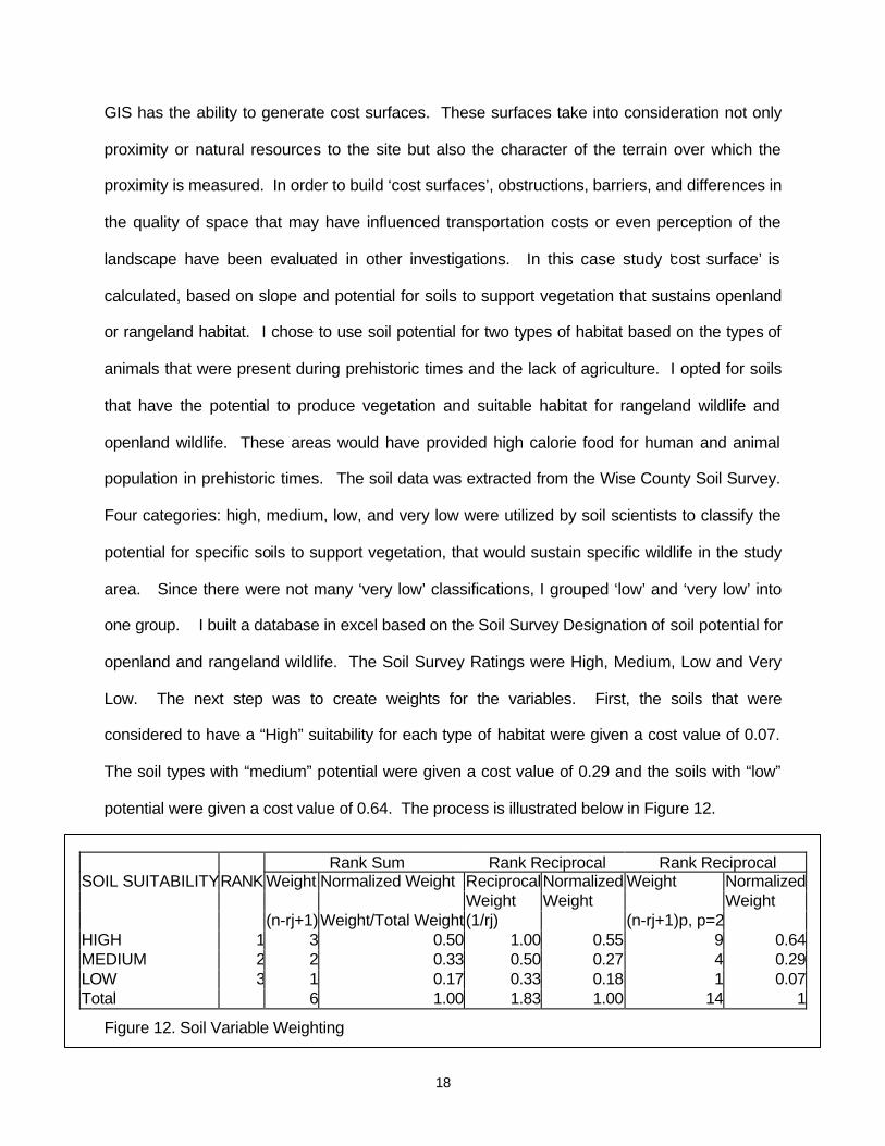
Low. The next step was to create weights for the variables. First, the soils that were
considered to have a “High” suitability for each type of habitat were given a cost value of 0.07.
The soil types with “medium” potential were given a cost value of 0.29 and the soils with “low”
potential were given a cost value of 0.64. The process is illustrated below in Figure 12.
Figure 12. Soil Variable Weighting
Rank Sum Rank Reciprocal Rank Reciprocal SOIL SUITABILITY RANK Weight Normalized Weight Reciprocal Normalized Weight Normalized Weight Weight Weight (n-rj+1)Weight/Total Weight (1/rj) (n-rj+1)p, p=2 HIGH 1 3 0.50 1.00 0.55 9 0.64MEDIUM 2 2 0.33 0.50 0.27 4 0.29LOW 3 1 0.17 0.33 0.18 1 0.07Total 6 1.00 1.83 1.00 14 1
19
These weights were derived by “Ranking Procedures” on page 180 of GIS and Multicriteria
Decision Analysis by Malczewski. In this continuous format, the cost of the soils could be
meaningfully combined with the slope values derived from the DEM of the study area. After
further deliberation and examination of the procedure for calculating Least Cost Path I chose to
rank my variables with whole numbers for the sake of simplicity and to save time. I plan to
choose continuous values for future studies but for the time being I decided to rank, reclassify,
and weight the variables to formulate the cost surface. As a result, soils with ‘high’ potential to
support the wildlife groups that I chose were given the lowest cost value of 1 and the ‘low’
potential areas were given the highest cost value of 3. Also, based on the fact that slopes are
not very steep in this region I grouped ‘slope impedance’ into three groups as well: steep,
medium and slight. Slopes were measured in degrees and based on the topography of this
area the slopes were classified into three groups according to Jenks natural breaks and then
reclassified with the steepest slopes given a cost value of ‘3’, the mid range values ‘2’, and the
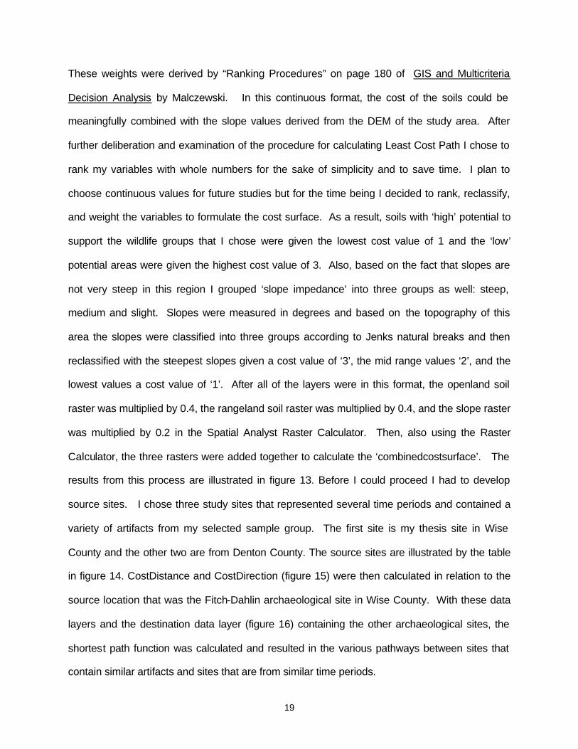
lowest values a cost value of ‘1’. After all of the layers were in this format, the openland soil
raster was multiplied by 0.4, the rangeland soil raster was multiplied by 0.4, and the slope raster
was multiplied by 0.2 in the Spatial Analyst Raster Calculator. Then, also using the Raster
Calculator, the three rasters were added together to calculate the ‘combinedcostsurface’. The
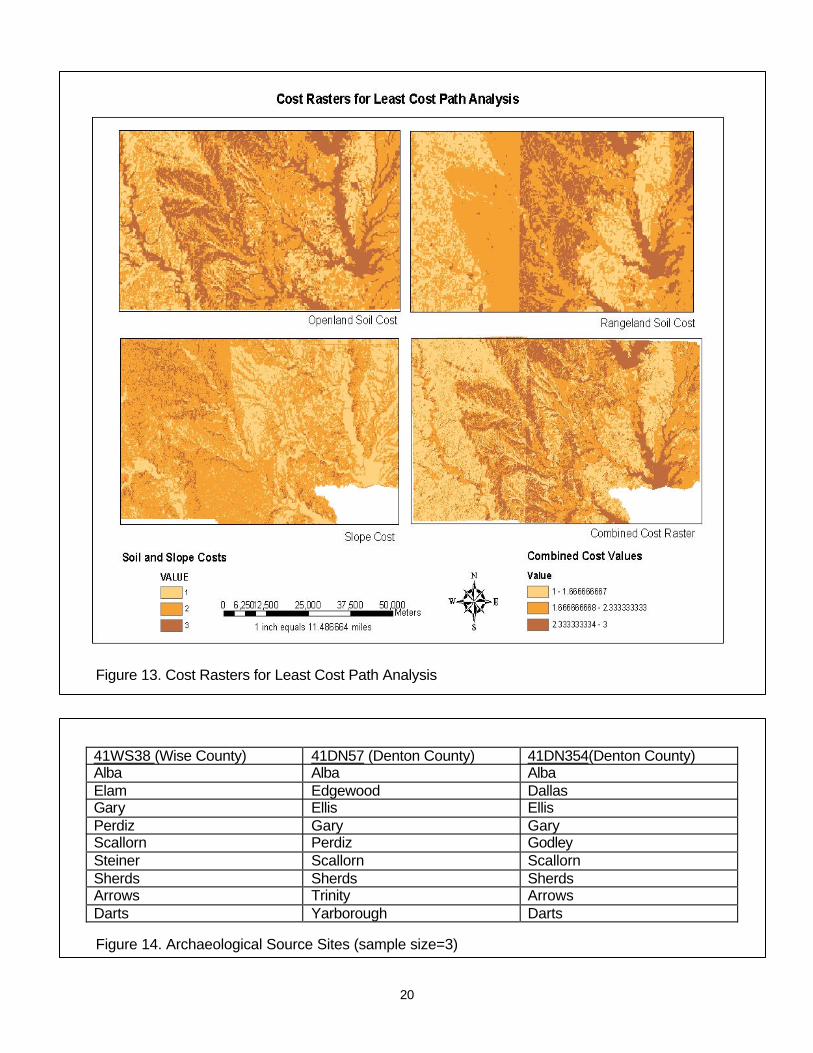
results from this process are illustrated in figure 13. Before I could proceed I had to develop
source sites. I chose three study sites that represented several time periods and contained a
variety of artifacts from my selected sample group. The first site is my thesis site in Wise
County and the other two are from Denton County. The source sites are illustrated by the table
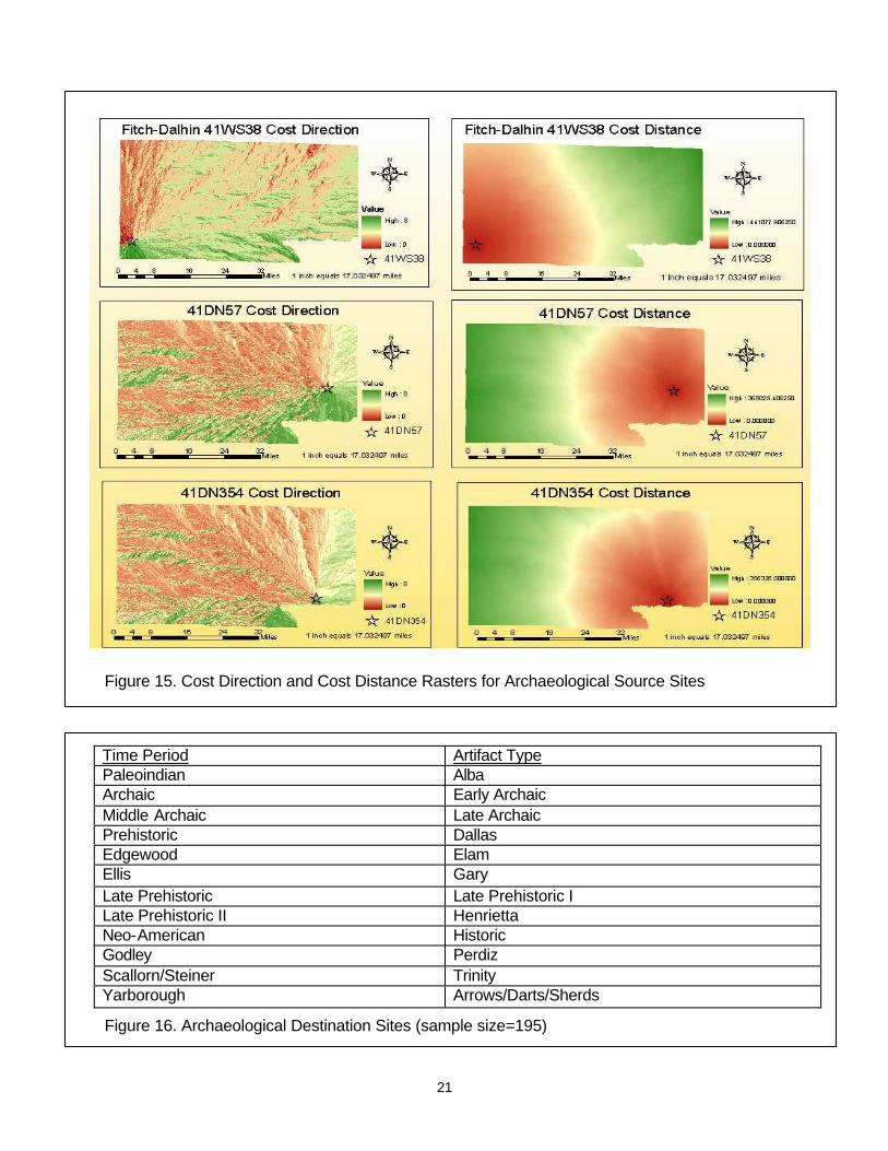
in figure 14. CostDistance and CostDirection (figure 15) were then calculated in relation to the
source location that was the Fitch-Dahlin archaeological site in Wise County. With these data
layers and the destination data layer (figure 16) containing the other archaeological sites, the
shortest path function was calculated and resulted in the various pathways between sites that
contain similar artifacts and sites that are from similar time periods.
20
Figure 13. Cost Rasters for Least Cost Path Analysis Figure 14. Archaeological Source Sites (sample size=3)
41WS38 (Wise County) 41DN57 (Denton County) 41DN354(Denton County) Alba Alba Alba Elam Edgewood Dallas Gary Ellis Ellis Perdiz Gary Gary Scallorn Perdiz Godley Steiner Scallorn Scallorn Sherds Sherds Sherds Arrows Trinity Arrows Darts Yarborough Darts
21
Figure 15. Cost Direction and Cost Distance Rasters for Archaeological Source Sites
Figure 16. Archaeological Destination Sites (sample size=195)
Time Period Artifact Type Paleoindian Alba Archaic Early Archaic Middle Archaic Late Archaic Prehistoric Dallas Edgewood Elam Ellis Gary Late Prehistoric Late Prehistoric I Late Prehistoric II Henrietta Neo-American Historic Godley Perdiz Scallorn/Steiner Trinity Yarborough Arrows/Darts/Sherds
22
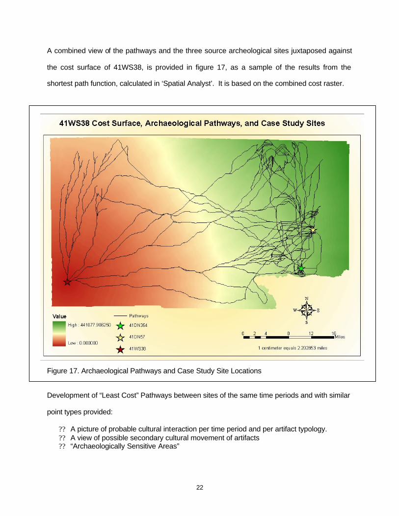
A combined view of the pathways and the three source archeological sites juxtaposed against
the cost surface of 41WS38, is provided in figure 17, as a sample of the results from the
shortest path function, calculated in ‘Spatial Analyst’. It is based on the combined cost raster.
Figure 17. Archaeological Pathways and Case Study Site Locations Development of “Least Cost” Pathways between sites of the same time periods and with similar
point types provided:
?? A picture of probable cultural interaction per time period and per artifact typology. ?? A view of possible secondary cultural movement of artifacts ?? “Archaeologically Sensitive Areas”
23
Several maps were built for analytical purposed in order to view this aspect in relation to time,
site distribution and the possibility of site interaction when sites contained the same artifacts or
were inhabited during the same time periods. Prehistoric sites have the largest distribution with
“intermediate” sites along the pathways. Once again, as with the RUSLE portion of the
analysis, the sample size seems to be distorting the picture.
Preliminary results suggest that there are strong correlations that merit further study and
refinement of this procedure. This study suggests that variables that created least cost
pathways facilitated reuse of specific site areas. Further study in developing site catchments,
and expanding the study area would be helpful in defining repeated occupation based on the
results of this analysis. In addition, travel-time between sites and within site catchment should
be factored into the equation. Beyond creating a more refined model, testing in the field is
necessary to evaluate the validity of pathways developed for this study and for future studies.
Site Selection: Overlay Analysis
In order to establish recommendations for CRM purposes I observed the interaction of past
and present cultures in combination with the character of the landscape. Overlay analysis
consisted of combining these data. The following goals were established for site selection:
?? Buffer Pathway Results by 100 meters. ?? Union all Pathway layers together and select pathways within city limits to be clipped. ?? Select “Archaeologically Sensitive” Zones based on Buffered Pathway Results. ?? Overlay city limits, land use, land cover, lakes, rivers, streams, and roads. ?? Determine why known sites are preserved to base selection of future “in situ” site areas. ?? Prioritize mitigation according to RUSLE Soil Erosion, Sinks, Pathways and Land Use.
Several of the goals were met but a few minor adjustments were made due to time factors.
Three “archaeologically sensitive” areas were chosen for preliminary cultural resource
management investigation. The primary selection criterion for site selection was pathway
density in relation to sinks and city limits. Figures 18 through 20 illustrate the areas selected for
cultural resource management survey and testing.

24
.Figure 18. Archaeological Pathways, Sinks, Roads and Case Study Site Location 'A'
25
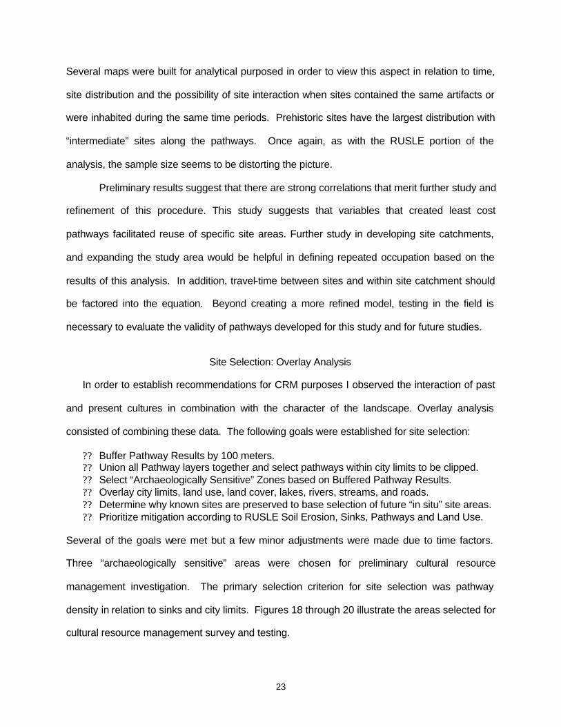
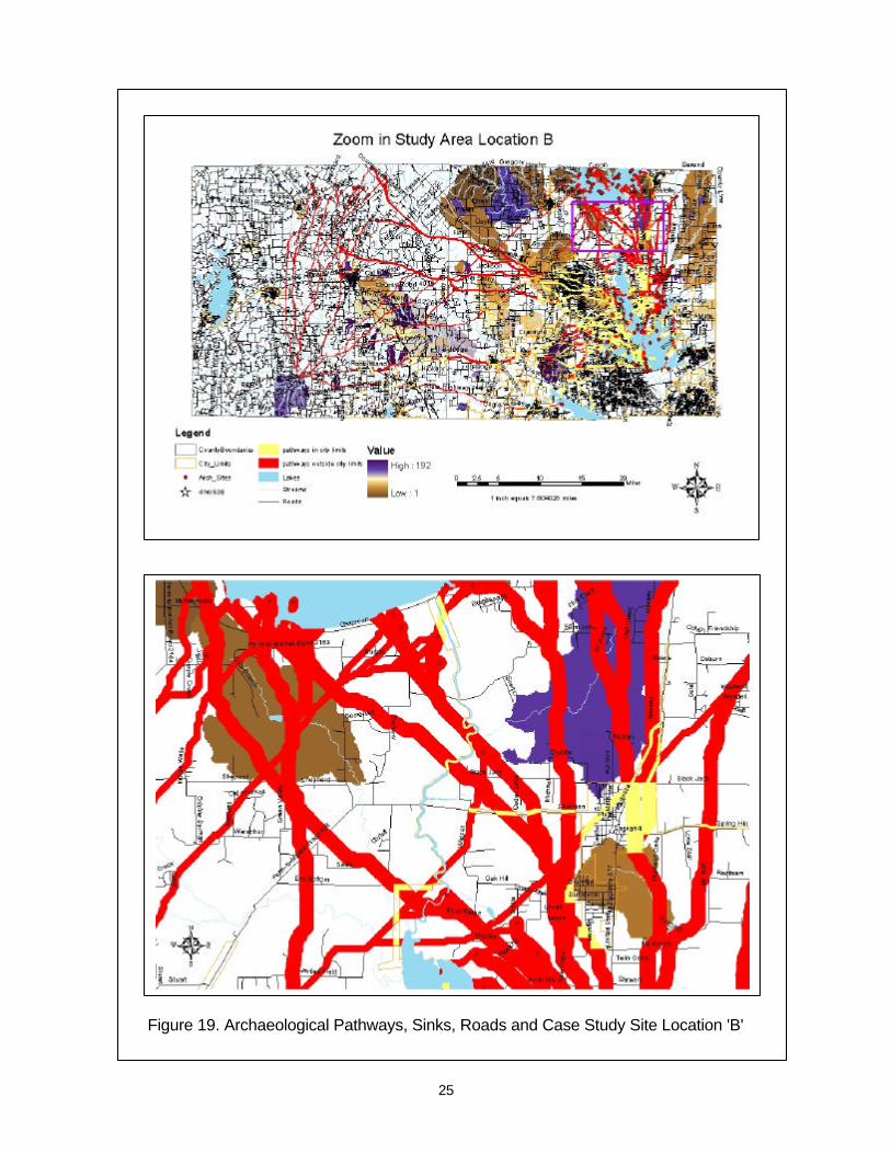
Figure 19. Archaeological Pathways, Sinks, Roads and Case Study Site Location 'B'

26
Figure 20. Archaeological Pathways, Sinks, Roads and Case Study Site Location 'C'

27
Once the areas are chosen, further inquiries can be made on a smaller scale with a GIS such as
selection of depth to bedrock, erosion values, aspect to observe the direction of sedimentation
flow, and variable sink depth to provide a game plan at a site level. The RUSLE calculation
provided information regarding areas of soil loss and increased sedimentation. The "Least Cost
Pathway" component of the analysis helped explain ancient behavioral choices in terms of site
location selection and facilitated the construction of ‘archaeological sensitive areas’. Overlay
analysis permitted observation of the interplay between these various components.
Conclusions
As a result of conducting this analysis it becomes more evident how GIS can benefit the
archaeological community and cultural resource managers. GIS, in the 'Information Age' is
becoming essential for cultural resource managers as an organizing mechanism as well as, for
identifying areas that may contain archaeological information for future planning and
preservation efforts. The combination of GIS techniques employed in this model appears to
have organizational potency, strong analytical utility, and predictive power. However, it needs to
be refined and pushed further in order to be more effective and attain greater accuracy.
Regional archaeological models, with predictive power could provide extremely useful tools to
governmental agencies responsible for the management and protection of archaeological
resources on public lands. Such models could be used for planning purposes, to indicate
archaeological sensitive regions where development or disturbance should be avoided, and
regions most likely lacking archaeological remains, where land alteration or development would
have less of an impact on the resource. Parker 1986 emphasizes the positive contribution
archaeological predictive modeling can make to resource management, through GIS, by
reducing costs and increasing the quality and efficiency of management. Moving a proposed
road alignment from a region predicted to be archaeologically sensitive, to one of less predicted
sensitivity, can lower the costs of mitigation of impacts, for example. Due to the fact that cultural
resource managers and government workers are often in charge of planning for and funding

28
archaeological resource recovery improvement of this GIS model would help maximize the
efficiency of the process of survey, excavation, preservation, and site selection for future
development.
Future Studies
Due to the scope of this analysis the need for further study is pronounced. In a cultural
resource management situation an additional layer of land parcel status would be very
beneficial so for future studies I would add that dimension. Prioritization, in that case would be
focused first on areas inside city limits that contain vacant parcels, sink areas, and pathways,
then outside city limits on areas that contain vacant parcels sink areas, and pathways, and
finally in areas where sinks and pathways overlap. ArcIMS would be a good mechanism for
communicating between entities and interacting with the data. In order to reach maximum
accuracy it would be necessary to include all of the sites recorded on file in the county. Also, a
site catchment analysis on these areas would provide more specific variables on which to
construct new pathways for greater accuracy. Other goals established for future research are
included as follows:
?? Develop datasets for county level archaeological studies to be distributed to city planners and cultural resource management agencies.
?? Overlay land parcels, determine how sites, site catchment areas and probable pathways relate to specific land parcels, wetlands, and water bodies.
?? Carry out field survey and excavations prior to completion of building permit process and construct new datasets in Excel Format to be submitted to archaeological “parent” agency.
?? Model needs refinement in variables and weights and travel time computations. ?? Develop “site catchment” profiles for sites. ?? On micro-scale, the arrangement of the archaeology within the site matrix needs more
attention. ?? On a meso-scale cultural resource managers need to be able to determine how the sites
relate to one another and to future development. ?? On a macro-scale there is a necessity to refine cultural resource management
techniques and facilitate comparisons between similar sites and environments.
In order to improve the models explored in this case study, and to enhance
archaeological analysis, I have proposed the addition of 'Site Catchment Analysis', for future
29
studies. Site Catchment Analysis is a technique that has been employed to analyze the
locations of archaeological sites with respect to the economic resources available to them. Site
Catchment Analysis derives from optimal foraging theory. The basic principle behind this
method is that the further from the base site the resources are, the greater the economic cost of
exploiting them. Eventually there is a point at which the cost of exploitation surpasses the
return. At this point an economic boundary can be defined to define the exploitation territory of
a site. The ability of GIS to extract a variety of information about the environment and perform
both geometric and statistical operations has led to its utility for the application of Site
Catchment Analysis in archaeology. In seeking explanations for the spatial patterning of cultural
remains archaeologists have concentrated on the distribution of sites and typically settlement
sites. As a result, a number of theoretical approaches have developed through time. A
prominent approach has been gravity models (Hodder and Orton 1976: 187-195). An economic
model of settlement structure was proposed by von Thunen in 1966. "Central Place" theories of
settlement hierarchy have been published in papers by Christaller (1935, 1966) and Grant
(1986a). Butzer's (1982) ecologically-based resource concentration models are also effective
explanatory mechanisms.
For the purposes of future research one of the central concerns will be “return to base”
cost and “accessibility” cost of site locations. In order to calculate site catchment areas in terms
of seasonal hunting and gathering behavior, the “return to base” cost will be derived by
implementation of the isotropic function. According to Wheatley and Gillings (2002),
“for the simplest case of isotropic cost surface calculation, the algorithm requires two inputs: a file containing the location of the features from which cost distance will be calculated (often referred to as seed locations) and a file that contains the cost of travel across each landscape unit is usually called a friction surface."
Slope, elevation, soil type and distance from specific natural resources should serve as the
most significant variables in terms of accessibility for generating friction surface. In addition, this
model will determine the pathways that incur the least cost and contain the least amount of

30
obstacles as a parameter for site selection. Friction data will be derived from generating slope
surface from an elevation map and then performing the selected transformation of slope surface
according to a proposed relationship between slope and time taken. In a case study, conducted
by Wheatley and Gillings (2002) F=1/log (slope+1) was used for illustration and then the cost
distance layer was reclassified according to the equation to identify zones that were within 2
hours walk. 'Return to base', Accessibility, and 'Distance' functions can help provide
explanations for why a site was visited on one occasion or repeatedly over a long period of time.
Based on a combination of the aforementioned methods, a more refined approach,
tailored to this area, for defining “catchment” areas, should be formulated, in future studies. Site
Catchment can be evaluated based on the character of the landscape that surrounds the site
locations. This type of analysis would help determine the variables that ancient inhabitants
would have considered the most advantageous. It would also provide strong base data that can
be weighted and utilized in the 'Weighted Distance', 'Shortest Path' and 'PATHDISTANCE' GIS
functions.
There are many answers to archaeological questions contained within GIS analytical
capacity, and ability to integrate data. GIS has been incorporated for handling and generating
vast amounts of spatial data, for performing analyses, developing, and testing locational
models, and for producing cartographic output in the form of archaeological predictive and other
maps over wide regions. (Marozas and Zack 1987; Warren et. al. 1987; Kvamme and Jochim
1989) This study was successful in terms of a 'pilot study' and developing methodology. I feel
like I have touched the 'tip of the iceberg' and it has created a sense of enthusiasm to make a
better model and retest. I plan to improve and evaluate this model in relation to my thesis to
help establish an explanatory mechanism for site location and examine the inter-site
relationships between sites in North Central Texas. The possibilities of expansion with respect
to this model, discovered during this analysis, provide a basis and increased confidence for the
success of future studies.
31
References
Butzer, Karl 1982. Archaeology as human ecology : method and theory for a contextual
approach. Cambridge ; New York : Cambridge University Press.
Ford, Alan, Ed Pauls, Milton Allen, Author Hanson, and J.O. McSpadden. 1980. Soil Survey of
Denton County, Texas. United States Department of Agriculture Soil Conservation Service in
Cooperation with Texas Agricultural Experiment Station.
Kohler and Parker 1986. Use of archaeological models in resource management contexts IN:
Advances in Archaeological Method and Theory volume 9. pg 286-287.
Kvamme, Kenneth L. 1989. Geographic Information Systems in Regional Archaeological
Research and Data Management. Archaeological Method and Theory,(Tucson) v. 1, pp.139-203
1990. The Fundamental Principles and Practice of Predictive Archaeological Modeling. IN:
Mathematics and Information Science in Archaeology: A Flexible Framework. (pg 257-295)
edited by Albertus Voorips. Holos—Verlag Bonn, Germany.
Malczewski, Jacek 1999. GIS and Multicriteria Decision Analysis. New York ; Chichester
[England] : John Wiley, c1999
Marozas, B. A., and J. A. Zack. 1990. GIS and Archaeological Site Location. Interpreting Space:
GIS and Archaeology. Chap. 14, Pp. 165-172. Allen, K., ed. Taylorand Francis. London..
Ressel, Dennis. D, Glen Ditmar, Edward Pauls, William M. Risinger, and Dennis F. Clower
1989. Soil Survey of Wise County, Texas. United States Department of Agriculture Soil
Conservation Service in Cooperation with Texas Agricultural Experiment Station.
Schiffer, Michael 1987. Formation processes of the archaeological record.
Albuquerque, NM : University of New Mexico Press.
Warren, R. E. 1990. Predictive Modelling in Archaeology: A Primer. Interpreting Space: GIS and
Archaeology. Chap. 9, Pp. 90-111. Allen, K., ed. Taylor and Francis. London.
Zeiler, Michael 1999. Modeling Our World: The ESRI Guide to Geodatabase Design. ESRI.
Top Related