


Languages
Pages
Legal


CS194-24Advanced Operating Systems
Structures and Implementation Lecture 21
Disks and FLASHQueueing Theory
April 21st, 2014Prof. John Kubiatowicz
http://inst.eecs.berkeley.edu/~cs194-24
Lec 21.24/21/14 Kubiatowicz CS194-24 ©UCB Fall 2014
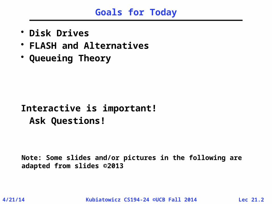
Goals for Today
• Disk Drives • FLASH and Alternatives• Queueing Theory
Interactive is important!Ask Questions!
Note: Some slides and/or pictures in the following areadapted from slides ©2013
Lec 21.34/21/14 Kubiatowicz CS194-24 ©UCB Fall 2014
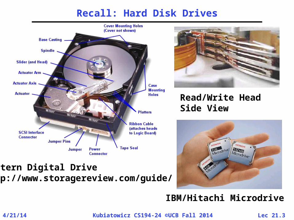
Recall: Hard Disk Drives
IBM/Hitachi Microdrive
Western Digital Drivehttp://www.storagereview.com/guide/
Read/Write HeadSide View
Lec 21.44/21/14 Kubiatowicz CS194-24 ©UCB Fall 2014
SectorTrack
Platter
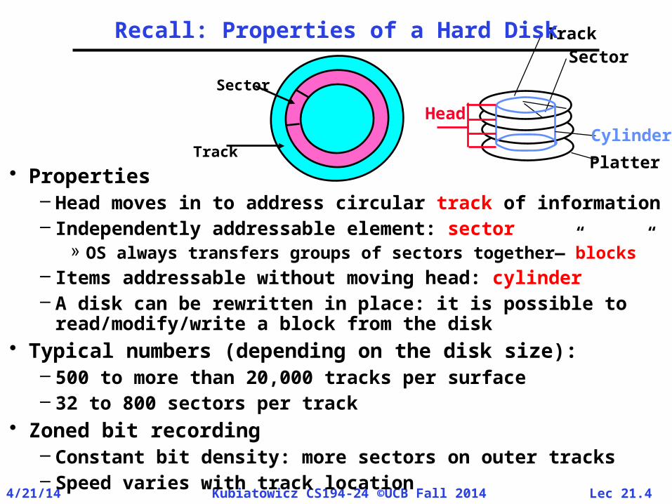
Recall: Properties of a Hard Disk
• Properties– Head moves in to address circular track of information– Independently addressable element: sector
» OS always transfers groups of sectors together—”blocks”– Items addressable without moving head: cylinder– A disk can be rewritten in place: it is possible to
read/modify/write a block from the disk• Typical numbers (depending on the disk size):
– 500 to more than 20,000 tracks per surface– 32 to 800 sectors per track
• Zoned bit recording– Constant bit density: more sectors on outer tracks– Speed varies with track location
Track
Sector
CylinderHead

Lec 21.54/21/14 Kubiatowicz CS194-24 ©UCB Fall 2014
Disk History
Data densityMbit/sq. in.
Capacity ofUnit ShownMegabytes
1973:1. 7 Mbit/sq. in140 MBytes
1979:7. 7 Mbit/sq. in2,300 MBytes
source: New York Times, 2/23/98, page C3, “Makers of disk drives crowd even mroe data into even smaller spaces”

Lec 21.64/21/14 Kubiatowicz CS194-24 ©UCB Fall 2014
Disk History
1989:63 Mbit/sq. in60,000 MBytes
1997:1450 Mbit/sq. in2300 MBytes
source: New York Times, 2/23/98, page C3, “Makers of disk drives crowd even mroe data into even smaller spaces”
1997:3090 Mbit/sq. in8100 MBytes

Lec 21.74/21/14 Kubiatowicz CS194-24 ©UCB Fall 2014
Recall: Seagate Hard Drive (2014)
• 6TB! 1000 Gb/in2
• 6 (3.5”) platters?, 2 heads each• Perpendicular recording• 7200 RPM, 4.16ms latency• 4KB sectors (512 emulation?)• 216MB/sec sustained
transfer speed• 128MB cache• Error Characteristics:
– MBTF: 1.4M hours– Bit error rate: 10-15
• Special considerations: – Normally need special “bios” (EFI): Bigger than easily
handled by 32-bit OSes.– Seagate provides special “Disk Wizard” software that
virtualizes drive into multiple chunks that makes it bootable on these OSes.

Lec 21.84/21/14 Kubiatowicz CS194-24 ©UCB Fall 2014
Nano-layered Disk Heads
• Special sensitivity of Disk head comes from “Giant Magneto-Resistive effect” or (GMR)
• IBM is (was) leader in this technology–Same technology as TMJ-RAM breakthrough
Coil for writing

Lec 21.94/21/14 Kubiatowicz CS194-24 ©UCB Fall 2014
Disk Figure of Merit: Areal Density
• Bits recorded along a track– Metric is Bits Per Inch (BPI)
• Number of tracks per surface– Metric is Tracks Per Inch (TPI)
• Disk Designs Brag about bit density per unit area– Metric is Bits Per Square Inch: Areal Density
= BPI x TPI
Year Areal Density1973 21979 81989 631997 3,0902000 17,1002006 130,0002007 164,0002009 400,0002010 488,0002014 1,000,000
1
10
100
1,000
10,000
100,000
1,000,000
1970 1980 1990 2000 2010
Are
al D
ensi
ty
Year
Lec 21.104/21/14 Kubiatowicz CS194-24 ©UCB Fall 2014
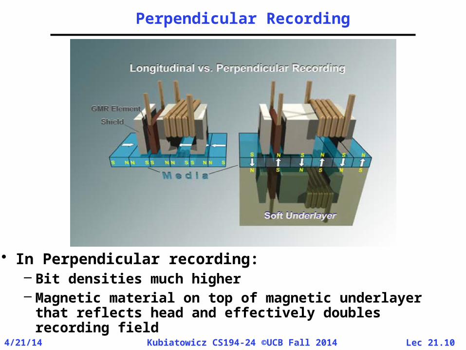
Perpendicular Recording
• In Perpendicular recording:– Bit densities much higher– Magnetic material on top of magnetic underlayer
that reflects head and effectively doubles recording field

Lec 21.114/21/14 Kubiatowicz CS194-24 ©UCB Fall 2014
Shingled Recording (Seagate/2014)
• Upside: Much denser recording – First generation seen as having 25% advantage– More to follow
• Downside: Need to rerecord multiple tracks at a time– Shingle grouping adapted to particular application– Great for log-structured/streaming writes!

Lec 21.124/21/14 Kubiatowicz CS194-24 ©UCB Fall 2014
Performance Model• Read/write data is a three-stage process:
– Seek time: position the head/arm over the proper track (into proper cylinder)
– Rotational latency: wait for the desired sectorto rotate under the read/write head
– Transfer time: transfer a block of bits (sector)under the read-write head
• Disk Latency = Queueing Time + Controller time +
Seek Time + Rotation Time + Xfer Time
• Highest Bandwidth: – Transfer large group of blocks sequentially from
one track
SoftwareQueue(Device Driver)
Hard
ware
Con
trolle
r Media Time(Seek+Rot+Xfer)
Req
uest
Resu
lt
Lec 21.134/21/14 Kubiatowicz CS194-24 ©UCB Fall 2014
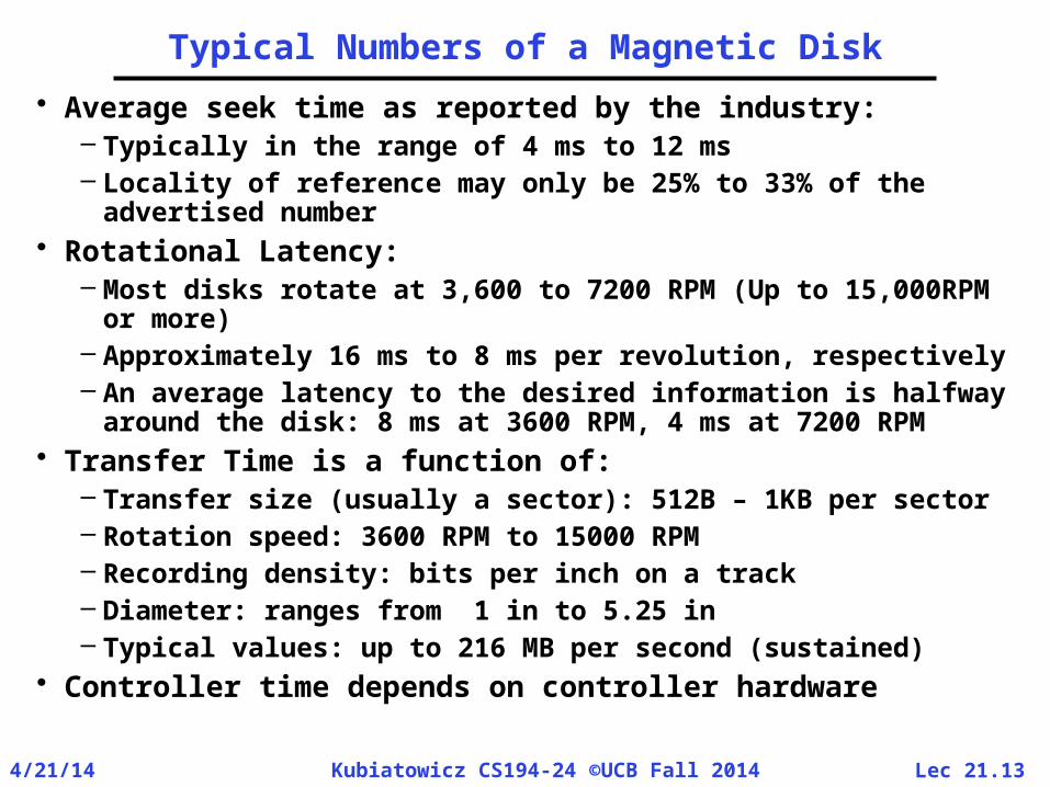
Typical Numbers of a Magnetic Disk
• Average seek time as reported by the industry:– Typically in the range of 4 ms to 12 ms– Locality of reference may only be 25% to 33% of the
advertised number• Rotational Latency:
– Most disks rotate at 3,600 to 7200 RPM (Up to 15,000RPM or more)
– Approximately 16 ms to 8 ms per revolution, respectively
– An average latency to the desired information is halfway around the disk: 8 ms at 3600 RPM, 4 ms at 7200 RPM
• Transfer Time is a function of:– Transfer size (usually a sector): 512B – 1KB per sector– Rotation speed: 3600 RPM to 15000 RPM– Recording density: bits per inch on a track– Diameter: ranges from 1 in to 5.25 in– Typical values: up to 216 MB per second (sustained)
• Controller time depends on controller hardware

Lec 21.144/21/14 Kubiatowicz CS194-24 ©UCB Fall 2014
Example: Disk Performance
• Question: How long does it take to fetch 1 Kbyte sector?
• Assumptions:– Ignoring queuing and controller times for now– Avg seek time of 5ms, avg rotational delay of 4ms– Transfer rate of 4MByte/s, sector size of 1 KByte
• Random place on disk:– Seek (5ms) + Rot. Delay (4ms) + Transfer (0.25ms)– Roughly 10ms to fetch/put data: 100 KByte/sec
• Random place in same cylinder:– Rot. Delay (4ms) + Transfer (0.25ms)– Roughly 5ms to fetch/put data: 200 KByte/sec
• Next sector on same track:– Transfer (0.25ms): 4 MByte/sec
• Key to using disk effectively (esp. for filesystems) is to minimize seek and rotational delays

Lec 21.154/21/14 Kubiatowicz CS194-24 ©UCB Fall 2014
Disk Scheduling• Disk can do only one request at a time; What
order do you choose to do queued requests?
• FIFO Order– Fair among requesters, but order of arrival may be
to random spots on the disk Very long seeks• SSTF: Shortest seek time first
– Pick the request that’s closest on the disk– Although called SSTF, today must include
rotational delay in calculation, since rotation can be as long as seek
– Con: SSTF good at reducing seeks, but may lead to starvation
• SCAN: Implements an Elevator Algorithm: take the closest request in the direction of travel– No starvation, but retains flavor of SSTF
• C-SCAN: Circular-Scan: only goes in one direction– Skips any requests on the way back– Fairer than SCAN, not biased towards pages in
middle
2,3
2,1
3,1
07,2
5,2
2,2 HeadUser
Requests
1
4
2
Dis
k H
ead
3

Lec 21.164/21/14 Kubiatowicz CS194-24 ©UCB Fall 2014
Linux Block Layer (Love Book, Ch 14)• Linux Block Layer
– Generic support for block-oriented devices
– Page Cache may hold data items
» On read, cache filled» On write, cache filled
before write occurs– Mapping layer
» Determines where physical blocks stored
– Generic Block Layer» Presents abstracted view
of block device» Ops represented by Block
I/O (“bio”) structures– I/O Scheduler
» Orders requests based on pre-defined policies
– Block Device Driver» Device-specific control
VFS
Disk Caches
DiskFilesyste
m
DiskFilesyste
m
BlockDevice
File
Generic Block Layer
I/O Scheduler Layer
Block DeviceDriver
Mapping Layer
Block DeviceDriver
Lec 21.174/21/14 Kubiatowicz CS194-24 ©UCB Fall 2014
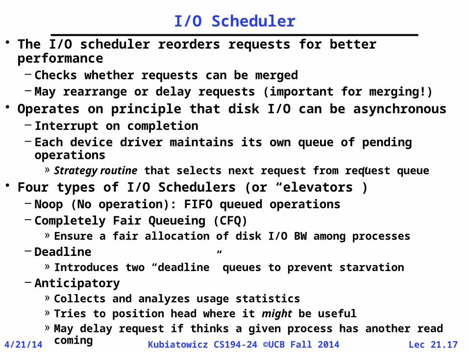
I/O Scheduler• The I/O scheduler reorders requests for better
performance– Checks whether requests can be merged– May rearrange or delay requests (important for merging!)
• Operates on principle that disk I/O can be asynchronous– Interrupt on completion– Each device driver maintains its own queue of pending
operations» Strategy routine that selects next request from request queue
• Four types of I/O Schedulers (or “elevators”)– Noop (No operation): FIFO queued operations– Completely Fair Queueing (CFQ)
» Ensure a fair allocation of disk I/O BW among processes– Deadline
» Introduces two “deadline” queues to prevent starvation– Anticipatory
» Collects and analyzes usage statistics» Tries to position head where it might be useful» May delay request if thinks a given process has another read
coming

Lec 21.184/21/14 Kubiatowicz CS194-24 ©UCB Fall 2014
What about other non-volatile options?
• There are a number of non-mechanical options for non-volatile storage– FLASH, MRAM, PCM
• Form Factors:– SSD (same form factor and interface as disk)– SIMMs/DIMMs
» May need to have device driver perform wear-leveling or other operations
• Advantages:– No mechanical parts (More reliable?)– Much less variability in access time than Disks
• Disadvantages:– FLASH “Wears out”– Cost/Bit still higher for alternatives
» The demise of spinning storage has been much overstated

Lec 21.194/21/14 Kubiatowicz CS194-24 ©UCB Fall 2014
FLASH Memory
• Like a normal transistor but:– Has a floating gate that can hold charge– To write: raise or lower wordline high enough to cause
charges to tunnel– To read: turn on wordline as if normal transistor
» presence of charge changes threshold and thus measured current
• Two varieties: – NAND: denser, must be read and written in blocks– NOR: much less dense, fast to read and write
Samsung 2007:16GB, NAND Flash

Lec 21.204/21/14 Kubiatowicz CS194-24 ©UCB Fall 2014
Evolution of FLASH (2014): Stacked Packaging
• Ultra-high memory densities: – E.g. 128 GB flash memory devices organized as 16-stack MCP
flash memory, with 64 Gb per die• Multi-channel I/O capability:
– E.g. 2 I/O channels can simultaneously process a read request and a write request (or 2 write requests, or 2 read requests).
– Samsung flash memory packages support a maximum of 4 I/O channels at a world-first.
• Very high thermal stability and operational reliability: – Samsung's advanced processes for packaging all types of flash
memory ensure that the device operates consistently and reliably under extreme temperature conditions
Lec 21.214/21/14 Kubiatowicz CS194-24 ©UCB Fall 2014
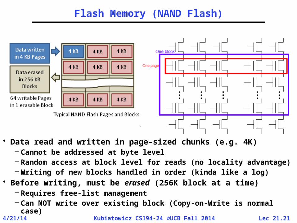
Flash Memory (NAND Flash)
• Data read and written in page-sized chunks (e.g. 4K)– Cannot be addressed at byte level– Random access at block level for reads (no locality advantage)– Writing of new blocks handled in order (kinda like a log)
• Before writing, must be erased (256K block at a time)– Requires free-list management– Can NOT write over existing block (Copy-on-Write is normal
case)

Lec 21.224/21/14 Kubiatowicz CS194-24 ©UCB Fall 2014
Flash Details
• Program/Erase (PE) Wear– Permanent damage to gate oxide at each flash cell– Caused by high program/erase voltages– Issues: trapped charges, premature leakage of charge– Need to balance how frequently cells written: “Wear Leveling”
• Flash Translation Layer (FTL)– Translates between Logical Block Addresses (at OS level) and
Physical Flash Page Addresses– Manages the wear and erasure state of blocks and pages– Tracks which blocks are garbage but not erased
• Management Process (Firmware)– Keep freelist full, Manage mapping, Track wear state of pages– Copy good pages out of basically empty blocks before erasure
• Meta-Data per page:– ECC for data– Wear State

Lec 21.234/21/14 Kubiatowicz CS194-24 ©UCB Fall 2014
Uses of FLASH for Storage
• SSD: Disk drive form factor with FLASH media– 800GB All FLASH– On-board wear-leveling– FLASH Management, erase, write,
read optimization– Garbage-collection done internally
• Hybrid Drive: FLASH+DISK– Example: Seagate SSHD (Mid 2014)
» 600GB Disk, 32GB FLASH, 128MB RAM
– According to Seagate: » Only promots hot data and
extends NAND life» Addresses performance
bottlenecks by caching at the I/O level
» Enables faster write response time» Helps ensure data integrity during
unexpected power loss

Lec 21.244/21/14 Kubiatowicz CS194-24 ©UCB Fall 2014
• Tunneling Magnetic Junction RAM (TMJ-RAM)– Speed of SRAM, density of DRAM, non-volatile
(no refresh)– “Spintronics”: combination quantum spin and
electronics– Same technology used in high-density disk-drives
Tunneling Magnetic Junction (MRAM)

Lec 21.254/21/14 Kubiatowicz CS194-24 ©UCB Fall 2014
Phase Change memory (IBM, Samsung, Intel)
• Phase Change Memory (called PRAM or PCM)– Chalcogenide material can change from amorphous
to crystalline state with application of heat– Two states have very different resistive properties – Similar to material used in CD-RW process
• Exciting alternative to FLASH– Higher speed– May be easy to integrate with CMOS processes

Lec 21.264/21/14 Kubiatowicz CS194-24 ©UCB Fall 2014
Queueing Behavior
• Performance of disk drive/file system– Metrics: Response Time, Throughput– Contributing factors to latency:
» Software paths (can be looselymodeled by a queue)
» Hardware controller» Physical disk media
• Queuing behavior:– Leads to big increases of latency
as utilization approaches 100% 100%
ResponseTime (ms)
Throughput (Utilization)(% total BW)
0
100
200
300
0%

Lec 21.274/21/14 Kubiatowicz CS194-24 ©UCB Fall 2014
Background: Use of random distributions
• Server spends variable time with customers– Mean (Average) m1 = p(T)T– Variance 2 = p(T)(T-m1)2 =
p(T)T2-m1 = E(T2)-m1– Squared coefficient of variance: C = 2/m12
Aggregate description of the distribution.• Important values of C:
– No variance or deterministic C=0 – “memoryless” or exponential C=1
» Past tells nothing about future» Many complex systems (or aggregates)
well described as memoryless – Disk response times C 1.5 (majority seeks <
avg)• Mean Residual Wait Time, m1(z):
– Mean time must wait for server to complete current task
– Can derive m1(z) = ½m1(1 + C)» Not just ½m1 because doesn’t capture variance
– C = 0 m1(z) = ½m1; C = 1 m1(z) = m1
Mean (m1)
mean
Memoryless
Distributionof service times

Lec 21.284/21/14 Kubiatowicz CS194-24 ©UCB Fall 2014
A Little Queuing Theory: Some Results• Assumptions:
– System in equilibrium; No limit to the queue– Time between successive arrivals is random and
memoryless
• Parameters that describe our system:– : mean number of arriving customers/second– Tser: mean time to service a customer (“m1”)– C: squared coefficient of variance = 2/m12
– μ: service rate = 1/Tser– u: server utilization (0u1): u = /μ = Tser
• Parameters we wish to compute:– Tq: Time spent in queue– Lq: Length of queue = Tq (by Little’s law)
• Results:– Memoryless service distribution (C = 1):
» Called M/M/1 queue: Tq = Tser x u/(1 – u)– General service distribution (no restrictions), 1 server:
» Called M/G/1 queue: Tq = Tser x ½(1+C) x u/(1 – u))
Arrival Rate
Queue ServerService Rateμ=1/Tser
Lec 21.294/21/14 Kubiatowicz CS194-24 ©UCB Fall 2014
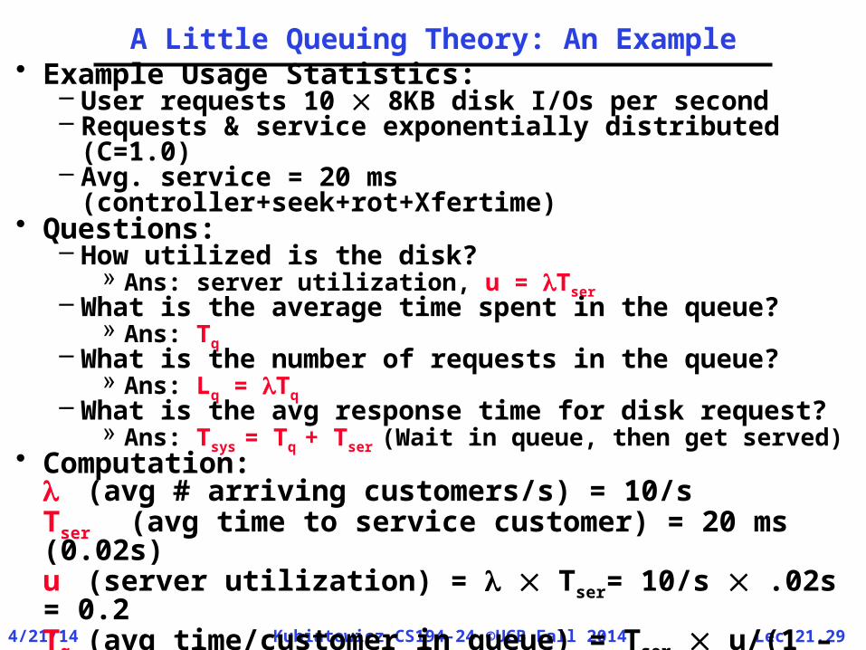
A Little Queuing Theory: An Example• Example Usage Statistics:
– User requests 10 8KB disk I/Os per second– Requests & service exponentially distributed
(C=1.0)– Avg. service = 20 ms
(controller+seek+rot+Xfertime)• Questions:
– How utilized is the disk? » Ans: server utilization, u = Tser– What is the average time spent in the queue? » Ans: Tq– What is the number of requests in the queue? » Ans: Lq = Tq– What is the avg response time for disk request? » Ans: Tsys = Tq + Tser (Wait in queue, then get served)
• Computation: (avg # arriving customers/s) = 10/sTser (avg time to service customer) = 20 ms (0.02s)u (server utilization) = Tser= 10/s .02s = 0.2Tq (avg time/customer in queue) = Tser u/(1 – u)
= 20 x 0.2/(1-0.2) = 20 0.25 = 5 ms (0 .005s)Lq (avg length of queue) = Tq=10/s .005s = 0.05Tsys (avg time/customer in system) =Tq + Tser= 25 ms

Lec 21.304/21/14 Kubiatowicz CS194-24 ©UCB Fall 2014
Summary
• Disk Storage: Cylinders, Tracks, Sectors– Access Time: 4-12ms– Rotational Velocity: 3600—15000 – Transfer Speed: Up to 200MB/sec
• Disk Time = queue + controller + seek + rotate +
transfer• Advertised average seek time benchmark
much greater than average seek time in practice
• Other Non-volatile memories– FLASH: packaged as SSDs or Raw SIMMs– MRAM, PCM, other options
• Queueing theory: for (c=1):
u
uxCW
1
121
u
uxW
1
Top Related