


Languages
Pages
Legal


BSB07
CREATE AND USE
SPREADSHEETS
BSBITU202A

CREATE AND USE SPREADSHEETS
BSBITU202A
To the learner UNIT PURPOSE Provide the participant with basic knowledge and skills to use a spreadsheet package effectively
LEARNING PLAN (suggested) Topic/Feature
Week
(3 hour lessons)
Occupational Health and Safety, Spreadsheet Terminology, Excel Screen, Mouse Pointer, On-Line Help, Theory Create a Worksheet (enter labels, column headings, text, numbers and dates)
1
Open, edit/change and resave data Format. Insert, delete a row and column, change column width Create a header and footer. Borders, fill colour and font colour Row height and text alignment. Wrap and vertically align text
2
Autosum, copying formula using autofill, format to currency Create a workbook and change worksheet name Functions (SUM, AVERAGE, MINIMUM, MAXIMUM) Data Series
3
Calculations and formula Order of operations, entering a formula, mathematical operators Print in landscape, centre vertically and horizontally
4
Show/hide formula, print selected cells Absolute and relative cell references Charts
5
Revision 6
Assessment (2 hours) 7
HOW YOU WILL BE ASSESSED
To be considered competent in this Unit you will need to:
• Read through the module and if you feel you are already competent, you may ask the trainer for an EXIT TEST
• Complete sufficient exercises in your Log Sheet PLUS pass the final assessment task at the end of the module
The assessment for this subject is recorded as COMPETENT/NOT YET COMPETENT and no marks are recorded centrally. Your results will be reported on your Transcript of Academic Record as COMPETENT/NOT YET COMPETENT

CREATE AND USE SPREADSHEETS
LOG SHEET
NAME ................................................ CLASS ...................................
TOPIC
EXERCISE
DATE COMPLETED
Occupational Health and Safety practices, Spreadsheet Terminology, Excel Screen, Mouse Pointer, On-Line Help, Theory
Read and note On-Line Help (Complete) Theory (Complete)
CREATE A WORKSHEET - Enter labels, column headings, text and numbers
BUSFARE, FLOORSPACE, KMRATE and HOLIDAY
Open, edit/change and resave data Format Insert, delete a row/column Create a header and footer Borders, colour, row height and text alignment
BUSFARE, FLOORSPACE, KMRATE and HOLIDAY OUTGEAR
Autosum, copying formula using autofill Format to currency Using workbooks
BUSFARE, FLOORSPACE, KMRATE and HOLIDAY
Workbook - TOTAL - COLES, MUSIC, MARKS
Format a Worksheet Sort a Worksheet
Exercise - PAPER
Functions (SUM, AVERAGE, MINIMUM, MAXIMUM)
Workbook - FUNCTION - COLES, MUSIC, MARKS, STUDENT
Data Series
SERIES
TOPIC
EXERCISE
DATE COMPLETED
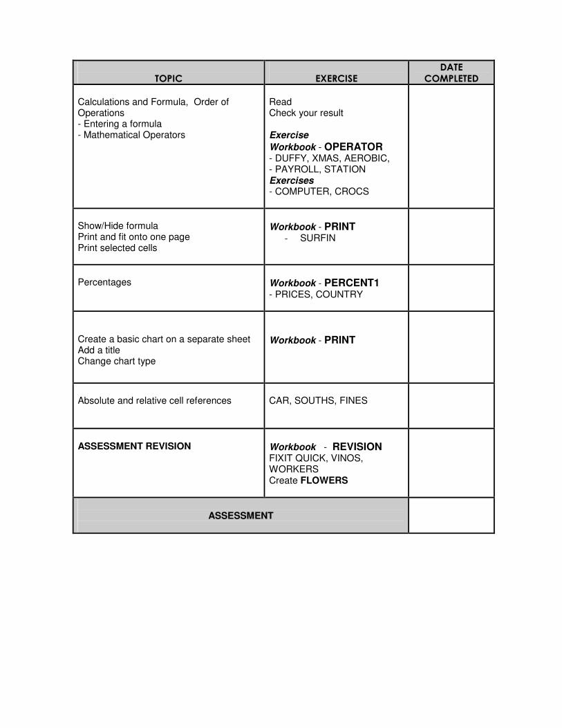
Calculations and Formula, Order of Operations - Entering a formula - Mathematical Operators
Read Check your result Exercise
Workbook - OPERATOR - DUFFY, XMAS, AEROBIC, - PAYROLL, STATION Exercises - COMPUTER, CROCS
Show/Hide formula Print and fit onto one page Print selected cells
Workbook - PRINT - SURFIN
Percentages
Workbook - PERCENT1 - PRICES, COUNTRY
Create a basic chart on a separate sheet Add a title Change chart type
Workbook - PRINT
Absolute and relative cell references
CAR, SOUTHS, FINES
ASSESSMENT REVISION
Workbook - REVISION FIXIT QUICK, VINOS, WORKERS Create FLOWERS
ASSESSMENT

TAFE NSW Hunter Institute Page 1 of 64 Faculty of Business and Computing Updated June 2009
LO1 USE RELEVANT OCCUPATIONAL HEALTH AND
SAFETY PRACTICES
Commonwealth and State legislation requires that all office environments adopt occupational health and
safety practices. The employer must provide a safe and healthy environment and the employee is
responsible for establishing safe working habits.
ERGONOMICS The study of the relationship between workers and their working environment. Ergonomic design and its correct use results in increased work efficiency, decreased fatigue, reduced health and injury problems and increased work satisfaction.
WORKSTATION A workstation consists of a chair, desk, document holder, footrest and computer. All elements of the workstation should be adjusted to suit the user: Correct posture should be demonstrated when sitting at the workstation.
Chair - height and back support � feet flat on floor � ankle, knees and hips at right angles � support lower back with back of the chair � back straight
Table � adjust height of desk so elbows are at right angles to keyboard � tops of legs should be just below table
Screen - tilt and brightness � keep screen brightness to a minimum � tilt the screen so that it may be viewed comfortably
Desk-top layout � clear desk of all unnecessary materials � use a document holder for your working papers to avoid neck strain
Power access � to avoid personal injury, ensure all electrical leads and computer cables are out of the way

TAFE NSW Hunter Institute Page 2 of 64 Faculty of Business and Computing Updated June 2009
Rest breaks and exercise periods � do some exercises or move away from the screen for 5 minutes every hour � stretch and relax fingers at least five times � blink eyes to rest and give them relief � lift shoulders upwards, backwards then relax them for one minute each � clasp hands above head, reach upwards, fingers interlaced, stretch, then drop arms � stand with feet slightly apart, hands in small of back, bend backwards, knees straight, hold for
two seconds
Activity
Please adjust your own workstation
Activity
START EXCEL
�
• Click on START
BUTTON
• START MENU appears
• Click on PROGRAMS
• Select from cascading menu
Activity
LEAVE EXCEL
Office Button, Close - when dialogue box appears, choose No to exit without saving the workbook You will return to the Windows desktop or
Click on the Close icon at the top right hand corner of the Excel window
TAFE NSW Hunter Institute Page 3 of 64 Faculty of Business and Computing Updated June 2009
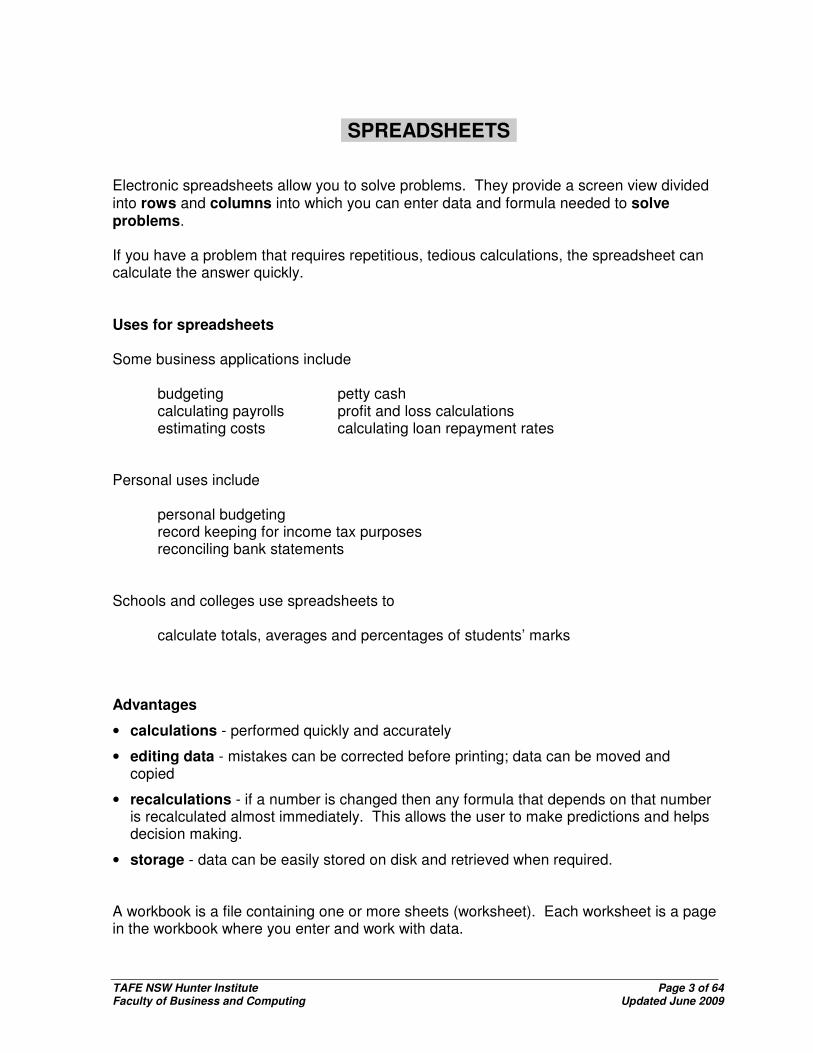
SPREADSHEETS Electronic spreadsheets allow you to solve problems. They provide a screen view divided into rows and columns into which you can enter data and formula needed to solve problems. If you have a problem that requires repetitious, tedious calculations, the spreadsheet can calculate the answer quickly. Uses for spreadsheets Some business applications include budgeting petty cash calculating payrolls profit and loss calculations estimating costs calculating loan repayment rates Personal uses include personal budgeting record keeping for income tax purposes reconciling bank statements Schools and colleges use spreadsheets to calculate totals, averages and percentages of students’ marks Advantages
• calculations - performed quickly and accurately
• editing data - mistakes can be corrected before printing; data can be moved and copied
• recalculations - if a number is changed then any formula that depends on that number is recalculated almost immediately. This allows the user to make predictions and helps decision making.
• storage - data can be easily stored on disk and retrieved when required. A workbook is a file containing one or more sheets (worksheet). Each worksheet is a page in the workbook where you enter and work with data.
TAFE NSW Hunter Institute Page 4 of 64 Faculty of Business and Computing Updated June 2009
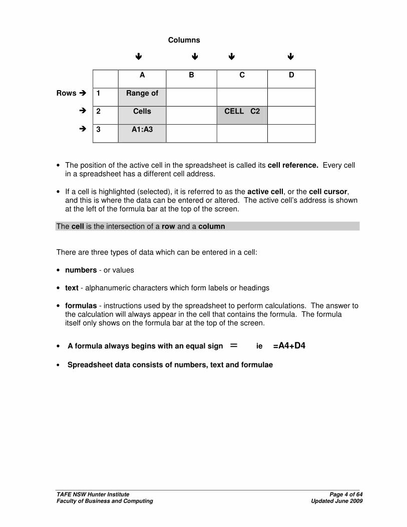
Columns
���� ���� ���� ����
A B C D
Rows � 1 Range of
� 2 Cells CELL C2
� 3 A1:A3
• The position of the active cell in the spreadsheet is called its cell reference. Every cell
in a spreadsheet has a different cell address. • If a cell is highlighted (selected), it is referred to as the active cell, or the cell cursor,
and this is where the data can be entered or altered. The active cell’s address is shown at the left of the formula bar at the top of the screen.
The cell is the intersection of a row and a column There are three types of data which can be entered in a cell: • numbers - or values • text - alphanumeric characters which form labels or headings • formulas - instructions used by the spreadsheet to perform calculations. The answer to
the calculation will always appear in the cell that contains the formula. The formula itself only shows on the formula bar at the top of the screen.
• A formula always begins with an equal sign = ie =A4+D4
• Spreadsheet data consists of numbers, text and formulae

TAFE NSW Hunter Institute Page 5 of 64 Faculty of Business and Computing Updated June 2009
THE EXCEL SCREEN
Office Button
Cell Reference Area
Formula Bar
Title Bar
Ribbon Split Box Horizontally
Start Button
Worksheets Scroll Bar
Zoom Slider
Worksheet Window

TAFE NSW Hunter Institute Page 6 of 64 Faculty of Business and Computing Updated June 2009
EXCEL SCREEN COMPONENTS
The Office Button The Office Button holds the commonly used functions in all the Microsoft applications. The common functions of New, Open, Save, Print, Close, etc are located here. Title Bar
Shows name of application - Microsoft Excel and name of workbook.
Quick Access Toolbar
The Quick Access toolbar holds three buttons: Save, Undo and Redo. You can also add other buttons that you use often but we do not cover that at this level. The Ribbon
The ribbon holds all the functions grouped together onto Tabs. Anything you want to do with your text can be carried out through these tabs. The Home tab holds the commonly used functions for formatting cells and basic functions for working with data.
The Insert tab holds the buttons used to add pictures, charts, tables, etc to your spreadsheet.
Scroll Bars Used to move up, down, left or right in worksheet. Formula Bar As you type data in an active cell, it also appears in the Formula bar. Also, the cell reference (A2) and the Enter � and Cancel � boxes are displayed.
Home
Insert

TAFE NSW Hunter Institute Page 7 of 64 Faculty of Business and Computing Updated June 2009
Worksheet Tabs A worksheet is selected by clicking once on relevant tab. Three sheets are usually contained in a workbook but you can add as many as required. Useful for keeping related information together. Minimise, Maximise and Close a Workbook
When a window is active it shows three buttons at the top right hand corner. The bottom buttons refer to the current worksheet and the top ones apply to the entire Spreadsheet Application.
Minimise Close Maximise
���� USING THE MOUSE
Click Press left or right mouse button once (usually left mouse button). Double Click Rapidly press left button twice. Used to access programs, open files etc Click and Drag Hold left mouse button while dragging the cursor over a set of cells to select them
TAFE NSW Hunter Institute Page 8 of 64 Faculty of Business and Computing Updated June 2009
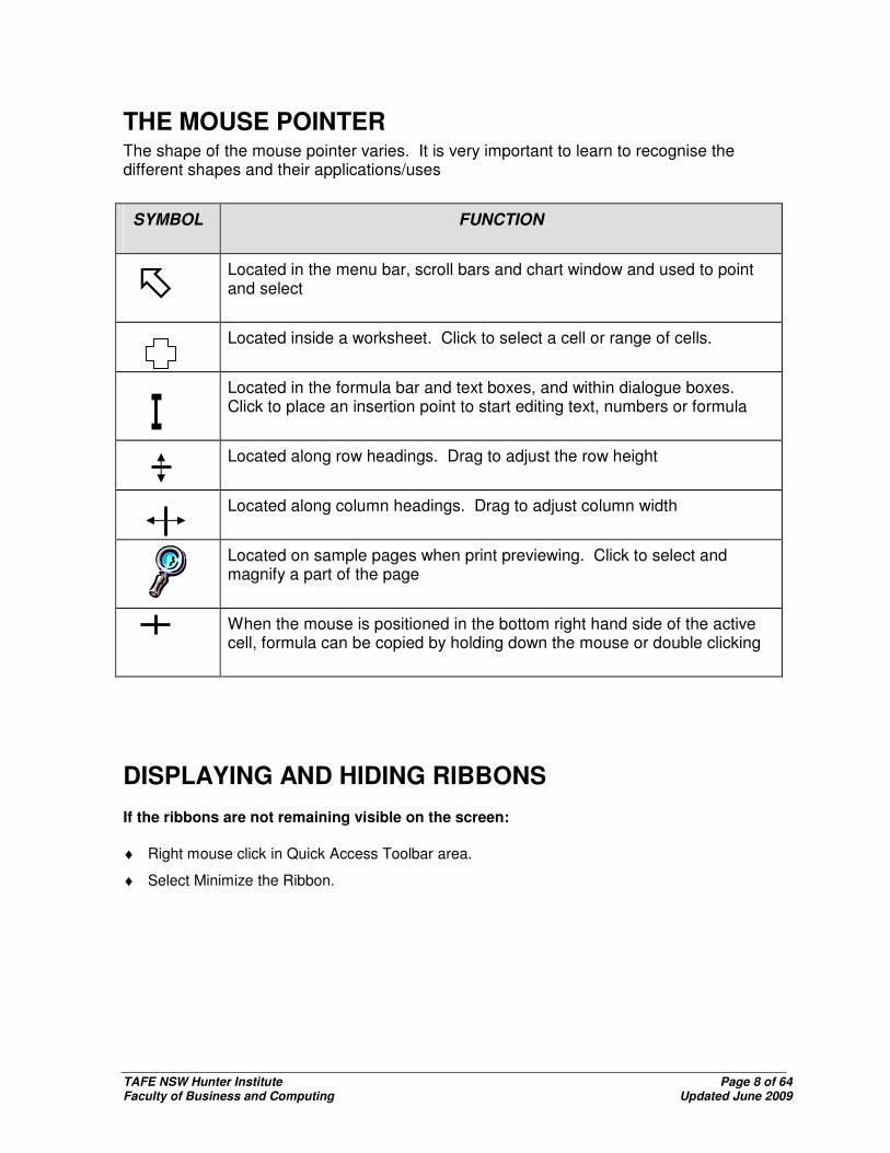
THE MOUSE POINTER The shape of the mouse pointer varies. It is very important to learn to recognise the different shapes and their applications/uses
SYMBOL
FUNCTION
Located in the menu bar, scroll bars and chart window and used to point and select
Located inside a worksheet. Click to select a cell or range of cells.
Located in the formula bar and text boxes, and within dialogue boxes. Click to place an insertion point to start editing text, numbers or formula
Located along row headings. Drag to adjust the row height
Located along column headings. Drag to adjust column width
Located on sample pages when print previewing. Click to select and magnify a part of the page
When the mouse is positioned in the bottom right hand side of the active cell, formula can be copied by holding down the mouse or double clicking
DISPLAYING AND HIDING RIBBONS If the ribbons are not remaining visible on the screen: ♦ Right mouse click in Quick Access Toolbar area.
♦ Select Minimize the Ribbon.

TAFE NSW Hunter Institute Page 9 of 64 Faculty of Business and Computing Updated June 2009
♦ Activity QUESTIONS
Examine the worksheet above and answer the following questions: What is the name of the Worksheet?.......................
What row is the column label Gross Wages on?
............................................................................ What is the cell reference for Zapper, M? ...............
How many columns contain data? .......................
What is the cell reference for the active cell?...........
What cell contains a formula? .............................
Is D4 a value, label or formula?................................
What row has a border? ......................................
What is contained in the range A5 to A10?
.................................................................................
What information is displayed in the formula bar?
............................................................................

TAFE NSW Hunter Institute Page 10 of 64 Faculty of Business and Computing Updated June 2009
Check your answers What is the name of the Worksheet? CROC
What row is the column label Gross Wages on? 4
What is the cell reference for Zapper, M? A10
How many columns contain data? 4
What is the cell reference for the active cell? D10
What cell contains a formula? D10 (any cell in the range C5:D10)
Is D4 a value, label or formula? Label
What row has a border? 4
What is contained in the range A5 to A10? Row Labels - Employee’s names
What information is displayed in the formula bar? =B10-C10 (formula to subtract Income Tax from Gross Wages)
Use Manuals and On-Line Help to Solve Operational Problems
Help Feature
To open help on your screen click on the Microsoft Help Button or press F1. You can then type in the search box the topic you require assistance with. Type in your question using plain English then click on SEARCH.
Activity
Type in your questions in the box provided: What is a formula? – click on SEARCH – double click on enter a formula to calculate a value – click on the printer icon at top of screen to print the topic What is a worksheet? – click on SEARCH – double click on about workbooks and worksheets – click on the printer icon at top of screen to print the topic

TAFE NSW Hunter Institute Page 11 of 64 Faculty of Business and Computing Updated June 2009
CREATING A WORKSHEET
ENTER ROW AND COLUMN LABELS, TEXT AND NUMBERS
SHOW ME HOW EXERCISE BUSFARE.XLS
ENTER DATA INTO A WORKSHEET: An entry made into a cell is either a label, number or formula. Text is called a label, headings are a common form of label entry and can be comprised of letters and/or numbers. Text is automatically left aligned and numbers (also called values) are automatically right aligned. ♦ Click on the cell where data is to appear ♦ Type in the data ♦ Confirm the data entry by pressing [ENTER] or any of the cursor movement keys - �������� CORRECTING MISTAKES If you make a mistake while you are entering data you can:
• press the <BACKSPACE> key then retype the data
• stop the entry by clicking the button in the Formula Bar
• press the <ESC> key If you have already accepted the cell entry:
• click on the cell and retype the whole entry OR • press <F2> and edit within the cell
CREATE A WORKSHEET Activity
Click on the Office Button and select New and enter the data below: Note: the text appears left aligned and the numbers right aligned.
A B C D E F
1 BUS ROUTE AUG SEPT OCT NOV DEC
2 University-Belmont 2430 1544 1128 3055 1245
3 Newcastle-Wallsend 1215 1602 1724 2411 2602
4 Charlestown-Newcastle 1844 1745 2350 1985 2187
5 Newcastle-Swansea 2343 1677 1695 2245 2946
TAFE NSW Hunter Institute Page 12 of 64 Faculty of Business and Computing Updated June 2009
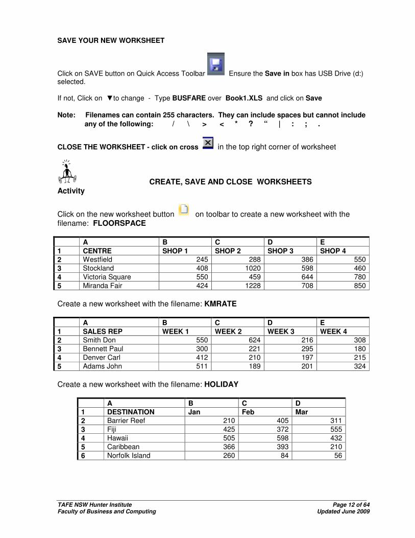
SAVE YOUR NEW WORKSHEET
Click on SAVE button on Quick Access Toolbar Ensure the Save in box has USB Drive (d:) selected. If not, Click on ▼to change - Type BUSFARE over Book1.XLS and click on Save Note: Filenames can contain 255 characters. They can include spaces but cannot include
any of the following: / \ > < * ? “ | : ; .
CLOSE THE WORKSHEET - click on cross in the top right corner of worksheet
CREATE, SAVE AND CLOSE WORKSHEETS Activity
Click on the new worksheet button on toolbar to create a new worksheet with the filename: FLOORSPACE
A B C D E
1 CENTRE SHOP 1 SHOP 2 SHOP 3 SHOP 4
2 Westfield 245 288 386 550
3 Stockland 408 1020 598 460
4 Victoria Square 550 459 644 780
5 Miranda Fair 424 1228 708 850
Create a new worksheet with the filename: KMRATE
A B C D E
1 SALES REP WEEK 1 WEEK 2 WEEK 3 WEEK 4
2 Smith Don 550 624 216 308
3 Bennett Paul 300 221 295 180
4 Denver Carl 412 210 197 215
5 Adams John 511 189 201 324
Create a new worksheet with the filename: HOLIDAY
A B C D
1 DESTINATION Jan Feb Mar
2 Barrier Reef 210 405 311
3 Fiji 425 372 555
4 Hawaii 505 598 432
5 Caribbean 366 393 210
6 Norfolk Island 260 84 56

TAFE NSW Hunter Institute Page 13 of 64 Faculty of Business and Computing Updated June 2009
SHOW ME HOW EXERCISE BUSFARE Open, Edit/Change and Resave a Worksheet
OPEN A WORKSHEET
• Click on the office button and select open - make sure you are in drive “d” (USB).
• Select/highlight filename BUSFARE • Click on Open OR double click filename EDIT/CHANGE DATA Move cursor to C5 Type in 1566 and press <ENTER> or use arrow key Move to F2, change to 2244 and press <ENTER> • YOUR WORKSHEET SHOULD NOW LOOK LIKE THIS
A B C D E F
1 BUS ROUTE AUG SEPT OCT NOV DEC
2 University-Belmont 2430 1544 1128 3055 2244
3 Newcastle-Wallsend 1215 1602 1724 2411 2602
4 Charlestown-Newcastle 1844 1745 2350 1985 2187
5 Newcastle-Swansea 2343 1566 1695 2245 2946
RESAVE WORKSHEET – Click on the save icon CLOSE THE WORKSHEET
Activity
Open, Edit/Change and Resave a Worksheet
OPEN THE WORKSHEET: FLOORSPACE
EDIT/CHANGE DATA Move cursor to C4 and change to 785 Move cursor to E3 and change to 640 RESAVE AND CLOSE THE WORKSHEET

TAFE NSW Hunter Institute Page 14 of 64 Faculty of Business and Computing Updated June 2009
OPEN THE WORKSHEET: KMRATE
EDIT/CHANGE DATA Move cursor to B5 and change to 155 Move cursor to D2 and change to 314 RESAVE AND CLOSE THE WORKSHEET
OPEN THE WORKSHEET: HOLIDAY
EDIT/CHANGE DATA Move cursor to B6 and change to 78 Move cursor to C3 and change to 480 RESAVE AND CLOSE THE WORKSHEET
SHOW ME HOW EXERCISE BUSFARE Formatting
CHANGE COLUMN WIDTH Procedure • Position cursor on vertical line between column letters (pointer
changes to black cross with arrows on horizontal bar)
• Click and drag to required width
• Repeat for all columns where required
ALIGN AND ENHANCE DATA
• Select/highlight all column headings
• Click on left, centre or right align icon on toolbar or
• Select/highlight date the click to bold, italicise or underline
TAFE NSW Hunter Institute Page 15 of 64 Faculty of Business and Computing Updated June 2009
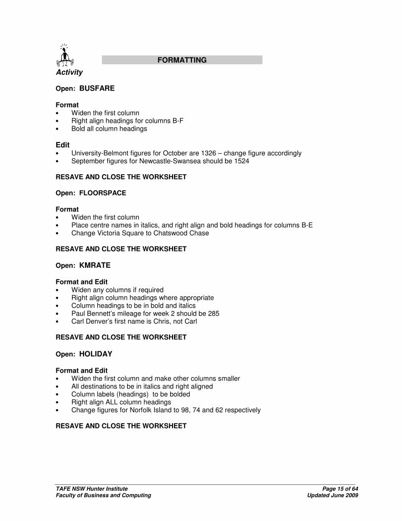
Activity
FORMATTING
Open: BUSFARE Format • Widen the first column • Right align headings for columns B-F • Bold all column headings
Edit • University-Belmont figures for October are 1326 – change figure accordingly • September figures for Newcastle-Swansea should be 1524 RESAVE AND CLOSE THE WORKSHEET Open: FLOORSPACE Format • Widen the first column • Place centre names in italics, and right align and bold headings for columns B-E • Change Victoria Square to Chatswood Chase RESAVE AND CLOSE THE WORKSHEET
Open: KMRATE Format and Edit • Widen any columns if required • Right align column headings where appropriate • Column headings to be in bold and italics • Paul Bennett’s mileage for week 2 should be 285 • Carl Denver’s first name is Chris, not Carl RESAVE AND CLOSE THE WORKSHEET
Open: HOLIDAY Format and Edit • Widen the first column and make other columns smaller • All destinations to be in italics and right aligned • Column labels (headings) to be bolded • Right align ALL column headings • Change figures for Norfolk Island to 98, 74 and 62 respectively RESAVE AND CLOSE THE WORKSHEET

TAFE NSW Hunter Institute Page 16 of 64 Faculty of Business and Computing Updated June 2009
SHOW ME HOW EXERCISE BUSFARE INSERT ROWS AND CENTRE HEADING OVER WORKSHEET
Procedure INSERT A ROW
• A new row will always be inserted above the active cell so ensure you have it placed correctly.
• From the Home ribbon select the insert button and then Insert Sheet Rows.
• Enter new data CENTRE THE HEADING OVER THE WORKSHEET • Select/highlight the cells containing the heading, drag mouse along the row to the last column
that contains data
• Click on the MERGE and CENTRE button on the Home ribbon
Activity
INSERT ROWS AND CENTRE THE HEADING OVER THE WORKSHEET
Open: BUSFARE • Add a blank row at the top of the worksheet • Insert a main heading in first column - SALES FOR HALF-YEAR - place in bold and italics • Centre the main heading over the columns • Insert a new row above Charlestown-Newcastle and enter the following data:
Shortland-Newcastle – 1505, 1640, 1668, 2535, 2602 RESAVE AND CLOSE THE WORKSHEET Open: FLOORSPACE • Add two new rows at the top of the worksheet • Insert a main heading in top row – SHOP FLOOR SPACE AVAILABLE – place in bold • Insert a subheading in second row – Measurements given in metres – in italics • Centre both the headings over the columns Hint: do one row at a time • Insert a blank row above Stockland and enter the following data;
Maroubra Junction – 322, 402, 266, 410 RESAVE AND CLOSE THE WORKSHEET
TAFE NSW Hunter Institute Page 17 of 64 Faculty of Business and Computing Updated June 2009
Open: KMRATE • Insert a blank row to separate column headings from column text • Insert two blank rows at top of worksheet • Enter a main heading – KILOMETRES TRAVELLED – bold and centre heading over columns RESAVE AND CLOSE THE WORKSHEET
Open: HOLIDAY • Insert a row above Hawaii • Enter the following data:
Solomon Islands – 29, 14, 35 • Insert a new row at beginning of worksheet • Enter a main heading – HOLIDAY DESTINATIONS – in bold and centre heading over
columns • Widen first column if required RESAVE AND CLOSE THE WORKSHEET
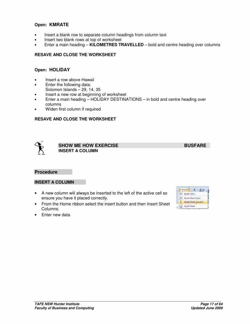
SHOW ME HOW EXERCISE BUSFARE INSERT A COLUMN
Procedure INSERT A COLUMN
• A new column will always be inserted to the left of the active cell so ensure you have it placed correctly.
• From the Home ribbon select the insert button and then Insert Sheet Columns.
• Enter new data

TAFE NSW Hunter Institute Page 18 of 64 Faculty of Business and Computing Updated June 2009
Activity
INSERT A COLUMN BUSFARE
Open: BUSFARE • Insert a new column at column B headed BUS NUMBER • Insert the following numbers into this column: Charlestown/Ncle - N228, Ncle/Swansea –
N350, Ncle/Wallsend – N232, Shortland/Ncle – N108, Uni/Belmont - N336 • Bus numbers are to be centred, along with the column heading • Add a heading TOTAL in column H. Format the heading so it is consistent with other column
headings RESAVE AND CLOSE THE WORKSHEET Open: FLOORSPACE • Insert a new column at column B headed OCCUPANCY RATE, widen the column if
necessary • Insert the following numbers into this column: 0.75, 0.8, 0.95, 0.85, 0.7. Centre figures in
column. Figures are NOT to be italicised. • Insert a new heading TOTAL after last column. Ensure it is formatted consistently. RESAVE AND CLOSE THE WORKSHEET
Open: KMRATE • Insert a new column at column A headed DEPARTMENT – re-centre main heading • Widen column and format heading so it is consistent with other column headings • Insert the following data into the new column – Haberdashery, Menswear, Toys, Kitchenware RESAVE AND CLOSE THE WORKSHEET
Open: HOLIDAY • Insert a new column at column B headed TOUR CODE, widen column if necessary • Insert the following tour codes into this column: BAR122, FIJ205, SOL196, HAW015,
CAR158, NOR010. Codes are not to be italicised • Insert new column at end headed TOTAL. Format heading so it is consistent with others • Re-centre main heading RESAVE AND CLOSE THE WORKSHEET

TAFE NSW Hunter Institute Page 19 of 64 Faculty of Business and Computing Updated June 2009
SORT FORMAT
SORT
SORT A WORKSHEET Procedure: Position cursor in any cell in column to be
sorted DO NOT HIGHLIGHT DATA Click on Sort and Filter in the Home Ribbon
and select either Sort A to Z for ascending order or Z to A for descending order
Hint: Excel can recognise column headings but it is best to insert a blank row between data and total rows before sorting
FORMAT
APPLY A BORDER, BACKGROUND COLOUR AND FONT COLOUR Procedure
•••• Select range:
� click on ▼ next to Border tool and choose style of border
� click on ▼ next to Fill Colour tool and choose a colour
� click on ▼ next to Font Colour tool and choose a colour for your text
Border Tool Fill Colour Tool
Font Colour Tool Font Size ALIGNMENT
WRAP TEXT IN CELL Text can be wrapped around a cell using the following button on the home ribbon:
TEXT ALIGNMENT Text is generally vertically aligned within a cell and can be changed using these buttons on the home ribbon:
Calibri ▼ 10 ▼
TAFE NSW Hunter Institute Page 20 of 64 Faculty of Business and Computing Updated June 2009
Activity
SORT FORMAT
BUSFARE
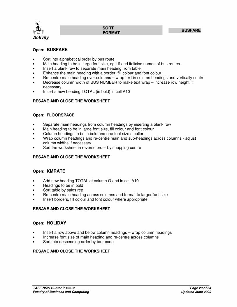
Open: BUSFARE • Sort into alphabetical order by bus route • Main heading to be in large font size, eg 16 and italicise names of bus routes • Insert a blank row to separate main heading from table • Enhance the main heading with a border, fill colour and font colour • Re-centre main heading over columns – wrap text in column headings and vertically centre • Decrease column width of BUS NUMBER to make text wrap – increase row height if
necessary • Insert a new heading TOTAL (in bold) in cell A10 RESAVE AND CLOSE THE WORKSHEET Open: FLOORSPACE • Separate main headings from column headings by inserting a blank row • Main heading to be in large font size, fill colour and font colour • Column headings to be in bold and one font size smaller • Wrap column headings and re-centre main and sub-headings across columns - adjust
column widths if necessary • Sort the worksheet in reverse order by shopping centre RESAVE AND CLOSE THE WORKSHEET
Open: KMRATE • Add new heading TOTAL at column G and in cell A10 • Headings to be in bold • Sort table by sales rep • Re-centre main heading across columns and format to larger font size • Insert borders, fill colour and font colour where appropriate RESAVE AND CLOSE THE WORKSHEET
Open: HOLIDAY • Insert a row above and below column headings – wrap column headings • Increase font size of main heading and re-centre across columns • Sort into descending order by tour code RESAVE AND CLOSE THE WORKSHEET

TAFE NSW Hunter Institute Page 21 of 64 Faculty of Business and Computing Updated June 2009
SHOW ME HOW EXERCISE BUSFARE INCREASE ROW HEIGHT CREATE A HEADER/FOOTER REMOVE BORDERS AND COLOUR
INCREASE ROW HEIGHT Procedure (read only)
� Highlight row/s in worksheet – black arrow on actual number (grey area) – drag down
� Position pointer on horizontal line between any two numbers
� Click and drag down until reference area displays required height and release mouse button
CREATE A HEADER and FOOTER Procedure (read only)
� Select the Insert ribbon
� Click on HEADER/FOOTER
� Header area will be split into three sections; left, middle and right
� Make your selection from the header and footer elements below or simply enter a choice of
your own
� To add a footer scroll down to the bottom of the page and press “click on to add footer”
� To return to your spreadsheet click anywhere in the worksheet area.
REMOVE BORDER AND COLOUR Procedure Remove border - select cells - choose No border from Border tool (5th icon in drop down box) Remove colour - select cells - choose Automatic from Colour Font tool

TAFE NSW Hunter Institute Page 22 of 64 Faculty of Business and Computing Updated June 2009
Activity
INCREASE ROW HEIGHT CREATE A HEADER/FOOTER REMOVE BORDERS AND COLOUR
BUSFARE
Open: BUSFARE • Click on the row numbers and increase row height to 22.5 • Insert a header – your name and the current date and insert a footer – the workbook
filename • Remove border and fill colour from the worksheet RESAVE AND CLOSE THE WORKSHEET Open: FLOORSPACE • Click on the row numbers and increase row height to 19.00 • Insert a header – the workbook filename and a footer – your name RESAVE AND CLOSE THE WORKSHEET
Open: KMRATE • Click on the row numbers and increase row height to 17.75 • Insert a footer - your name, the current date and the workbook filename RESAVE AND CLOSE THE WORKSHEET
Open: HOLIDAY • Click on the row numbers and increase row height to 21.00 • Insert a header – your name and the current date • Insert a footer – the workbook filename RESAVE AND CLOSE THE WORKSHEET

TAFE NSW Hunter Institute Page 23 of 64 Faculty of Business and Computing Updated June 2009
SHOW ME HOW EXERCISE OUTGEAR OPEN AN EXISTING FILE FROM P: DRIVE
Procedure
� Click on the Office button select open (or press Control + c)
� Click on P: drive
� Double click on BUSINESS then BUSINESS ADMINISTRATION then COMPUTING
� Click on ROUTINE SPREADSHEETS then TIGHES HILL MANUAL
� Double click on OUTGEAR.XLS
The file must now be saved to your D: drive
Activity
OPEN AN EXISTING FILE FROM P: DRIVE REVISION
OUTGEAR
Open: OUTGEAR
• Apply colour and borders, wrap column headings, bold and vertically align in cell
• Increase row height to 22.5 for all rows containing data
• Centre heading and sub-heading across worksheet, bold and increase point size to 18
• Insert a header (filename) and a footer (your name)
ENSURE YOUR FILE IS SAVED ON D: DRIVE AND CLOSE

TAFE NSW Hunter Institute Page 24 of 64 Faculty of Business and Computing Updated June 2009
SHOW ME HOW EXERCISE
AUTOSUM AND FORMAT TO CURRENCY COPYING FORMULA USING AUTOFILL
READ ONLY
AUTOSUM (on toolbar) will add either vertically or horizontally Procedure -.Position cursor in cell where total is to be inserted
- Click on - Area to be added is surrounded by a moving line
- Click on again to insert total. COPYING FORMULA USING AUTOFILL Procedure
- Position cursor in cell that contains the formula to be copied
- Move mouse pointer to bottom right hand corner of box (called the fill handle)
You will know you are in the correct position when pointer changes to a thinner black cross
- Drag fill handle down or across the cells where formula is to be copied to and release
FORMAT TO CURRENCY Procedure - Highlight column to be formatted
- Click on the drop down arrow next to general in the number formatting group
(located on the Home Ribbon).
- Select currency to have 2 decimal places and $ positioned next to numbers or select Accounting
to have 2 decimal places and $ spaced away from numbers

TAFE NSW Hunter Institute Page 25 of 64 Faculty of Business and Computing Updated June 2009
Activity
FORMULA (ADDING) FORMAT TO CURRENCY AUTOFILL
BUSFARE
Open: BUSFARE
• Use AUTOSUM to add the TOTAL column – calculate horizontal totals • Copy formula down • Insert formula at foot of August column to calculate totals for AUGUST. Copy formula across
remaining columns • Format all figures to currency (except BUS NUMBER) dollar sign next to numbers • Insert top and bottom border around column headings and also around TOTAL row. Add fill
colour to column headings
• Preview using Preview button, located in the office button under print. RESAVE AND CLOSE THE WORKSHEET Open: FLOORSPACE
• Use AUTOSUM to add the TOTAL column and copy formula down • Insert top and bottom border around column headings and add fill colour • Use another fill colour to highlight to Occupancy Rate column
• Click on the percentage button on the toolbar to format those cells to a percentage RESAVE AND CLOSE THE WORKSHEET
Open: KMRATE
• Use AUTOSUM to calculate horizontal and vertical totals • Sort into alphabetical order by Department RESAVE AND CLOSE THE WORKSHEET

TAFE NSW Hunter Institute Page 26 of 64 Faculty of Business and Computing Updated June 2009
SHOW ME HOW EXERCISE Using Workbooks
WORKBOOKS A workbook consists of a set of related sheets. Related data can be kept in one location. You can move around the workbook using the navigation buttons First Sheet Last Sheet
Previous Sheet Next Sheet To move a sheet within the same workbook � Select sheet tab you wish to move � Drag it to its new location (note triangle indicates position) � Release mouse button when triangle is in desired location Delete a sheet � With mouse positioned over sheet tab to be deleted, click right mouse button � Select Delete from the dialogue box Rename a sheet � With mouse positioned over sheet tab to be renamed, double click left mouse button � Existing name will be highlighted � Type the new name then press Enter

TAFE NSW Hunter Institute Page 27 of 64 Faculty of Business and Computing Updated June 2009
Activity
Using Workbooks - Autosum, Autofill and Currency
OPEN: the workbook TOTAL
• Click on worksheet tab COLES in bottom left-hand corner of screen to open ����
• Total the month of January using (Autosum) in the editing section of the home ribbon.
• Use Autofill to copy formula for all months
• Total the columns GROCERIES, MEATS, SUNDRIES and MONTHLY TOTAL
• Format to currency and apply borders, colour and/or pattern where appropriate
• Centre the heading and sub-heading across the worksheet,
• Bold and increase point size to 16
• All column headings should be vertically centred - MONTHLY TOTAL should be wrapped in box
Click on the MUSIC tab to open • Calculate the TOTAL SALES and ITEM TOTALS
• Change the sales of ALBUMS for JUL-SEPT - it should be 55500
• Insert a new column after SINGLES for COMPACT DISKS and enter the figures below:
JAN-MAR 40348 APR-JUN 53098
JUL-SEPT 43521 OCT-DEC 64890
• Auto-fill formulae across where necessary - check the TOTAL SALES to ensure range is
correct
• Apply right alignment, word-wrap and vertical centring to ALL column headings
• Apply italics and bold where desired and currency where appropriate
• Apply borders and colour and Increase row height to all cells containing data to 22.5
Click on the MARKS tab to open
• Calculate the total marks for each subject
• Change the row labels to italics and increase the row height to 22
• Bold, vertically centre and word-wrap column headings - apply borders appropriately
• Insert a new student ARNOLD - His marks are: Spreadsheet Fundamentals (66)
Database Fundamentals (79) Data Retrieval (89) and
Computer Operations (55)
• Insert a suitable title at the top of the worksheet, centred across worksheet and insert a blank
row under the title.
• Save and Close workbook TOTAL

TAFE NSW Hunter Institute Page 28 of 64 Faculty of Business and Computing Updated June 2009
Activity
FORMAT AND SORT A WORKSHEET
Filename: PAPER.XLS
• CREATE the worksheet as shown below:
A B C D E
1 PAPER DISTRIBUTORS LTD - SALES FIGURES
2
3 AREA SEPT OCT NOV TOTAL
4 CITY 6892 6412 6011
5 LAKE MACQUARIE 5831 4998 3532
6 UPPER HUNTER 2698 2846 2561
7 CENTRAL COAST 4325 4871 3996
8 MANNING 1675 2023 2174
9 TOTAL SALES
• Save the spreadsheet as PAPER.
• Ensure fields display all data. Use bold and italics where appropriate. Insert a border or fill colour to the main heading and centre over worksheet
• Calculate the total cost of each area (TOTAL) and auto-fill/copy down
• Calculate the TOTAL SALES - and click on twice.
• A mistake was made when compiling data - Lake Macquarie for November should be 6032.
• December figures have now been completed - Insert a column DEC and enter the following data:
City (7556) Lake Macquarie (5999) Upper Hunter (3012)
Central Coast (5050) Manning (3074)
Note: UPDATE TOTAL - click on again and fill down to include new data
• Insert a row between Lake Macquarie and Upper Hunter PORT STEPHENS and insert the following:
Sept (1568) Oct (1998) Nov (2020) Dec (4567)
Update TOTAL (use Autofill/fill handle)
• Delete a row - Central Coast has been included in the Sydney area.
• Use the Home Ribbon and go to the Number area to do the following

TAFE NSW Hunter Institute Page 29 of 64 Faculty of Business and Computing Updated June 2009
Format appropriate columns to currency - highlight cells first - click on on toolbar
Decrease the decimal places to 0 - select cells, click on decrease button on toolbar
• Insert blank row between data and TOTAL SALES
• Sort the spreadsheet in ascending order according to AREA (DO NOT HIGHLIGHT DATA)
• Resave and print the worksheet with the filename and your name in the footer
SHOW ME HOW EXERCISE
Functions
A function is a pre-written or in-built formula. All functions, like formulae, begin with an equal sign (=). Functions also include an argument plus a range in brackets after the function name.
The range has a colon (:) between the first and last cell, eg =SUM(A1:A3) Procedure - Active cell is where the result of the calculation is to appear - Key in equal sign and function name, plus range in brackets <ENTER> - Position cursor in cell that contains function to be copied - Position cursor in bottom right hand corner of cell (thin black cross) - Drag down or across range Example: =SUM(A5:A10) Adds the values in the range starting with A5 and ending with A10 The functions you will cover in this module are:
SUM =SUM(A5:A10) Example as above (usually inserted using the auto-sum
button ) AVERAGE =AVERAGE(A5:A10) Adds the values in the range, divides the total by number of values MINIMUM =MIN(A5:A10) Inserts the minimum/lowest value in the stipulated range MAXIMUM =MAX(A5:A10) Inserts the maximum/largest value in the stipulated range
Function name
Argument
TAFE NSW Hunter Institute Page 30 of 64 Faculty of Business and Computing Updated June 2009
OPEN THE WORKBOOK FUNCTION
Click on COLES tab
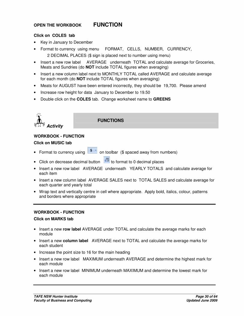
• Key in January to December
• Format to currency using menu FORMAT, CELLS, NUMBER, CURRENCY,
2 DECIMAL PLACES ($ sign is placed next to number using menu)
• Insert a new row label AVERAGE underneath TOTAL and calculate average for Groceries, Meats and Sundries (do NOT include TOTAL figures when averaging)
• Insert a new column label next to MONTHLY TOTAL called AVERAGE and calculate average for each month (do NOT include TOTAL figures when averaging)
• Meats for AUGUST have been entered incorrectly, they should be 19,700. Please amend
• Increase row height for data January to December to 19.50
• Double click on the COLES tab. Change worksheet name to GREENS
Activity
FUNCTIONS
WORKBOOK - FUNCTION
Click on MUSIC tab
• Format to currency using on toolbar ($ spaced away from numbers)
• Click on decrease decimal button to format to 0 decimal places
• Insert a new row label AVERAGE underneath YEARLY TOTALS and calculate average for each item
• Insert a new column label AVERAGE SALES next to TOTAL SALES and calculate average for each quarter and yearly total
• Wrap text and vertically centre in cell where appropriate. Apply bold, italics, colour, patterns and borders where appropriate
WORKBOOK - FUNCTION
Click on MARKS tab
• Insert a new row label AVERAGE under TOTAL and calculate the average marks for each module
• Insert a new column label AVERAGE next to TOTAL and calculate the average marks for each student
• Increase the point size to 16 for the main heading
• Insert a new row label MAXIMUM underneath AVERAGE and determine the highest mark for each module
• Insert a new row label MINIMUM underneath MAXIMUM and determine the lowest mark for each module
TAFE NSW Hunter Institute Page 31 of 64 Faculty of Business and Computing Updated June 2009
WORKBOOK - FUNCTION
Click on STUDENT tab
• Calculate horizontal and vertical totals
• Widen columns so they look less crowded
• Headings should be in bold and aligned with their respective column data
• Sort into ascending alphabetical order by student
• Add a new column (in Column G) headed AVERAGE. Calculate average mark for each student
• Add a new row at the end (in A10) headed AVERAGE. Calculate average for each subject
• Insert your name in a footer and the filename and date in the header and resave
•
SHOW ME HOW EXERCISE
Switching between open workbooks
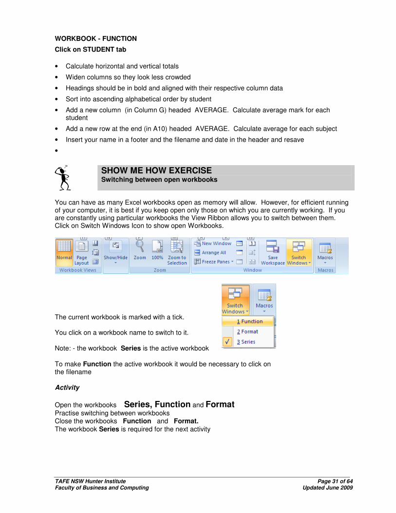
You can have as many Excel workbooks open as memory will allow. However, for efficient running of your computer, it is best if you keep open only those on which you are currently working. If you are constantly using particular workbooks the View Ribbon allows you to switch between them. Click on Switch Windows Icon to show open Workbooks.
The current workbook is marked with a tick. You click on a workbook name to switch to it. Note: - the workbook Series is the active workbook To make Function the active workbook it would be necessary to click on the filename Activity
Open the workbooks Series, Function and Format Practise switching between workbooks Close the workbooks Function and Format. The workbook Series is required for the next activity
TAFE NSW Hunter Institute Page 32 of 64 Faculty of Business and Computing Updated June 2009
SHOW ME HOW EXERCISE
Data Series
A data series is a series of values that you need in a worksheet, where the individual values are related to each other in a simple way eg series of dates, days, years, numbers. Procedure - Key in first of series eg Monday, January etc - Drag fill handle (Autofill) down or across the cells where series is to be copied to and release Note: This same method applies to dates, days, numbers etc. Just highlight enough cells
to set format
Activity
Data Series
Open: SERIES
USE AUTOFILL TO CREATE A SERIES FOR EACH COLUMN A series of months - key in first month, use autofill and drag down or across A series of numbers - 1,2,3 etc - type 1 - hold down <CTRL> when using autofill A series of time of day and days of the week - as for months A Series of numbers that are not consecutive (must key in first 2 numbers as example)
SHOW ME HOW EXERCISE
Calculations and Formula Mathematical Operators
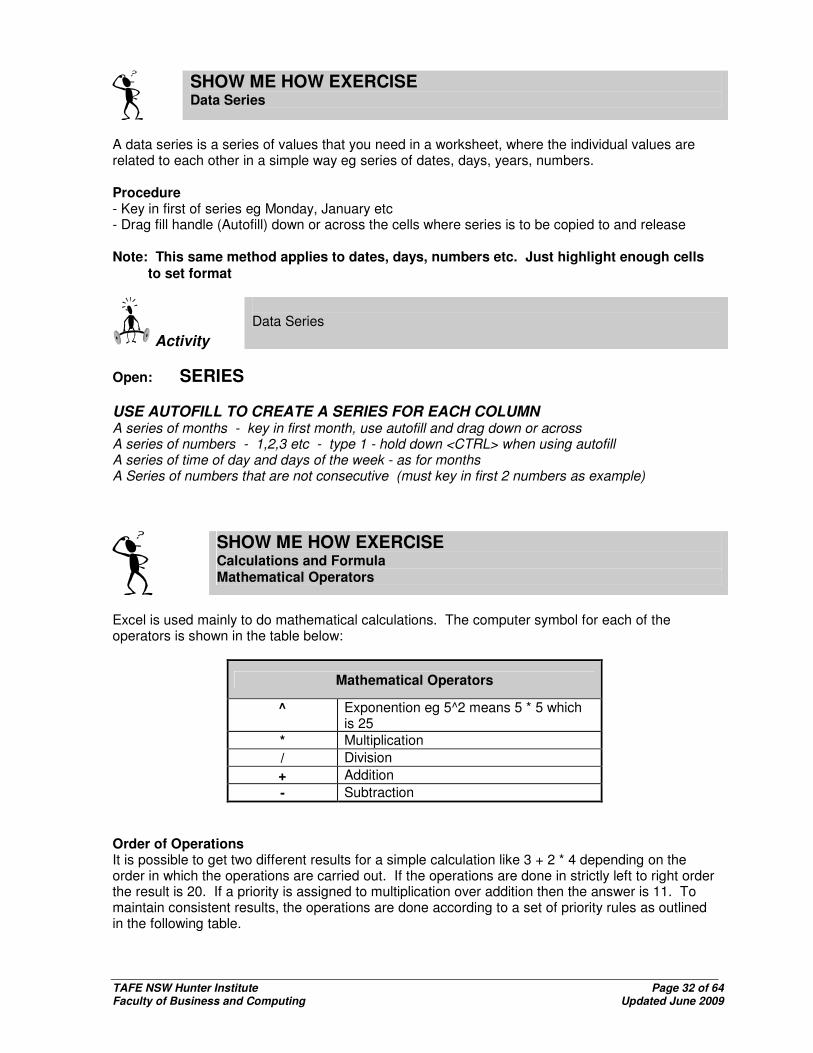
Excel is used mainly to do mathematical calculations. The computer symbol for each of the operators is shown in the table below:
Mathematical Operators
^ Exponention eg 5^2 means 5 * 5 which is 25
* Multiplication
/ Division
+ Addition
- Subtraction
Order of Operations It is possible to get two different results for a simple calculation like 3 + 2 * 4 depending on the order in which the operations are carried out. If the operations are done in strictly left to right order the result is 20. If a priority is assigned to multiplication over addition then the answer is 11. To maintain consistent results, the operations are done according to a set of priority rules as outlined in the following table.

TAFE NSW Hunter Institute Page 33 of 64 Faculty of Business and Computing Updated June 2009
Mathematical Operator Priority Rules
( ) Operations enclosed in parentheses are done first ^ Exponentions are done next from left to right * and / Multiplication and division are done next from left to
right + and - Additions and subtractions are done next from left to
right
Entering a Formula To enter a formula in an active cell, first press = (equal sign) to signify that what follows is a formula. Using the keys on the numeric keypad will make formula entries easier.
A
CHECK YOUR RESULT
1 =4+2*5 14
2 =(4+2)*5 30
3 =2*4+32/4-3 13
4 =2*(4+32)/4-3 15
5 =2*4+32/(4-3) 40
6 =2*(4+32)/(4-3) 72
7 =(2*4+32)/4-3 7
8 =(2*4+32)/(4-3) 40
Activity
Creating a workbook with multiple worksheets Calculations and Formula Mathematical Operators
Create the workbook MATHS Create and name the following worksheet Waratah • Calculate TOTAL for Price and Quantity only • Calculate TOTAL PRICE - insert formulae as indicated in D4 and Auto-fill down • Format to currency where appropriate
A B C D
1 Waratah Nursery
2
3 Type of Plant Price Quantity Total Price
4 Protea 7.55 20 =b4*c4
5 Banksia 6.95 15
6 Wattle 3.50 30
7 TOTAL
RESULT?
PRICE 18.00 QUANTITY 65 TOTAL PRICE Protea $151.00 Banksia $104.25 Wattle $105.00
TAFE NSW Hunter Institute Page 34 of 64 Faculty of Business and Computing Updated June 2009
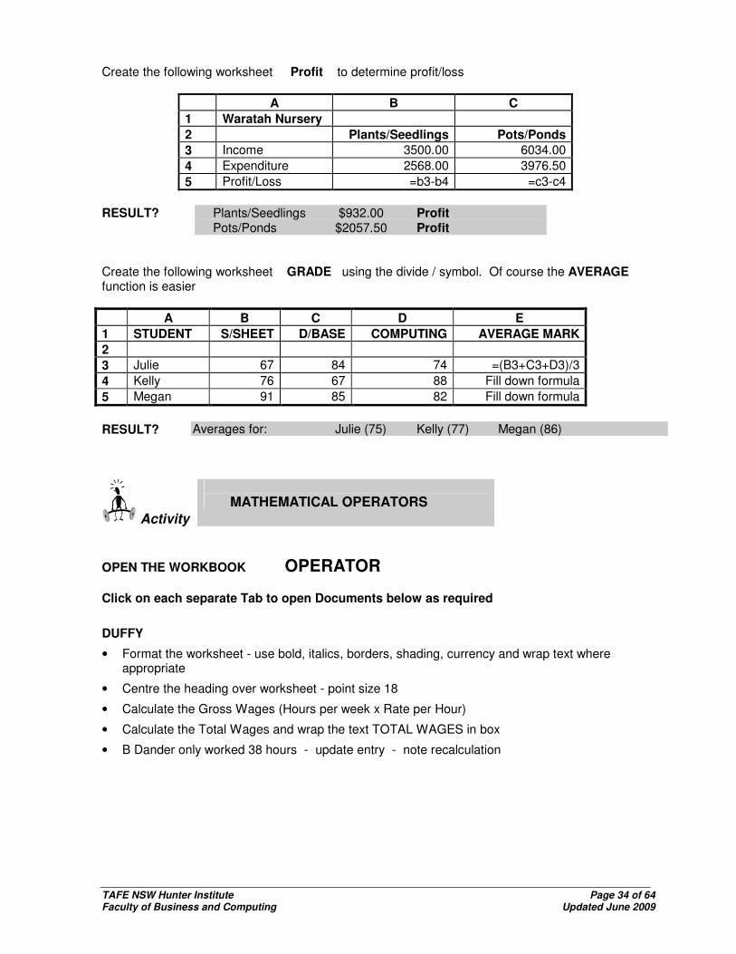
Create the following worksheet Profit to determine profit/loss
A B C
1 Waratah Nursery
2 Plants/Seedlings Pots/Ponds
3 Income 3500.00 6034.00
4 Expenditure 2568.00 3976.50
5 Profit/Loss =b3-b4 =c3-c4
RESULT? Plants/Seedlings $932.00 Profit
Pots/Ponds $2057.50 Profit
Create the following worksheet GRADE using the divide / symbol. Of course the AVERAGE function is easier
A B C D E
1 STUDENT S/SHEET D/BASE COMPUTING AVERAGE MARK
2
3 Julie 67 84 74 =(B3+C3+D3)/3
4 Kelly 76 67 88 Fill down formula
5 Megan 91 85 82 Fill down formula
RESULT? Averages for: Julie (75) Kelly (77) Megan (86)
Activity
MATHEMATICAL OPERATORS
OPEN THE WORKBOOK OPERATOR
Click on each separate Tab to open Documents below as required
DUFFY
• Format the worksheet - use bold, italics, borders, shading, currency and wrap text where appropriate
• Centre the heading over worksheet - point size 18
• Calculate the Gross Wages (Hours per week x Rate per Hour)
• Calculate the Total Wages and wrap the text TOTAL WAGES in box
• B Dander only worked 38 hours - update entry - note recalculation
TAFE NSW Hunter Institute Page 35 of 64 Faculty of Business and Computing Updated June 2009
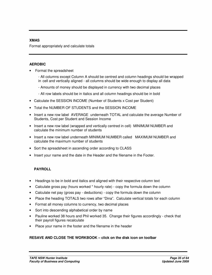
XMAS
Format appropriately and calculate totals
AEROBIC
• Format the spreadsheet
- All columns except Column A should be centred and column headings should be wrapped in cell and vertically aligned - all columns should be wide enough to display all data
- Amounts of money should be displayed in currency with two decimal places
- All row labels should be in italics and all column headings should be in bold
• Calculate the SESSION INCOME (Number of Students x Cost per Student)
• Total the NUMBER OF STUDENTS and the SESSION INCOME
• Insert a new row label AVERAGE underneath TOTAL and calculate the average Number of Students, Cost per Student and Session Income
• Insert a new row label (wrapped and vertically centred in cell) MINIMUM NUMBER and calculate the minimum number of students
• Insert a new row label underneath MINIMUM NUMBER called MAXIMUM NUMBER and calculate the maximum number of students
• Sort the spreadsheet in ascending order according to CLASS
• Insert your name and the date in the Header and the filename in the Footer.
PAYROLL
• Headings to be in bold and italics and aligned with their respective column text
• Calculate gross pay (hours worked * hourly rate) - copy the formula down the column
• Calculate net pay (gross pay - deductions) - copy the formula down the column
• Place the heading TOTALS two rows after “Dina”. Calculate vertical totals for each column
• Format all money columns to currency, two decimal places
• Sort into descending alphabetical order by name
• Pauline worked 38 hours and Phil worked 35. Change their figures accordingly - check that their payroll figures recalculate
• Place your name in the footer and the filename in the header
RESAVE AND CLOSE THE WORKBOOK – click on the disk icon on toolbar

TAFE NSW Hunter Institute Page 36 of 64 Faculty of Business and Computing Updated June 2009
STATION
• Calculate the gross profit (Sales - Cost of Sales) and copy formula down
• Calculate net profit (gross profit - expenses) and copy down
• Calculate the TOTALS row at bottom of worksheet
• Sort the worksheet in descending alphabetical order by OUTLET. Insert a blank row to separate main heading from column headings.
• Right align those headings which sit above figure columns. Place all column and row headings into italics and Times Roman font in a suitable size
• Format all figure columns as currency columns
• Place your name in the footer and the filename in the header
RESAVE AND CLOSE THE WORKBOOK
Activity
Consolidation Exercise
• CREATE the spreadsheet COMPUTER as shown below:
A B C D
1 COMPUTER ROOM -COSTS
2
3 ITEM UNIT COST NO OF UNITS TOTAL
4
5 Systems Unit 1500.00 12
6 Monitor 300.00 12
7 Keyboard 175.00 12
8 Desk 120.00 12
9 Chairs 99.00 12
10 Printers 620.00 2
11 Filing Cabinet 130.00 1
12 Whiteboard 800.00 1
13 TV Monitor 410.50 1
14 TOTAL COST
TAFE NSW Hunter Institute Page 37 of 64 Faculty of Business and Computing Updated June 2009
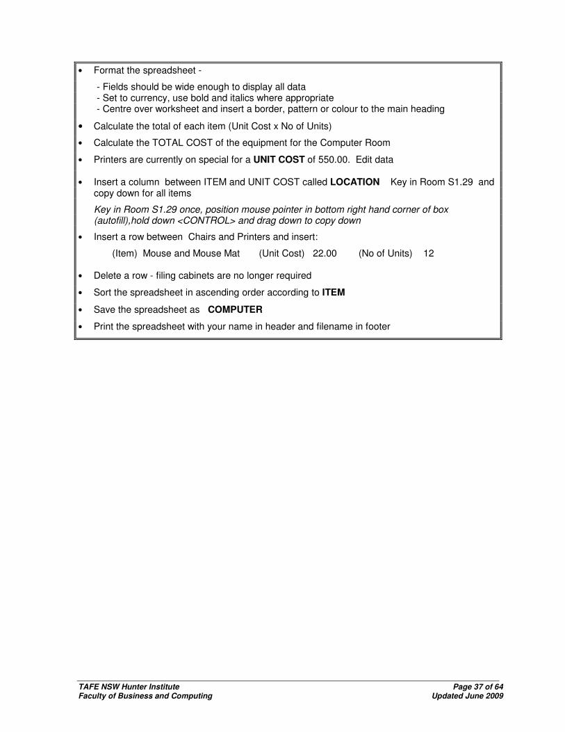
• Format the spreadsheet -
- Fields should be wide enough to display all data - Set to currency, use bold and italics where appropriate - Centre over worksheet and insert a border, pattern or colour to the main heading
• Calculate the total of each item (Unit Cost x No of Units)
• Calculate the TOTAL COST of the equipment for the Computer Room
• Printers are currently on special for a UNIT COST of 550.00. Edit data
• Insert a column between ITEM and UNIT COST called LOCATION Key in Room S1.29 and copy down for all items
Key in Room S1.29 once, position mouse pointer in bottom right hand corner of box (autofill),hold down <CONTROL> and drag down to copy down
• Insert a row between Chairs and Printers and insert:
(Item) Mouse and Mouse Mat (Unit Cost) 22.00 (No of Units) 12 • Delete a row - filing cabinets are no longer required
• Sort the spreadsheet in ascending order according to ITEM
• Save the spreadsheet as COMPUTER
• Print the spreadsheet with your name in header and filename in footer

TAFE NSW Hunter Institute Page 38 of 64 Faculty of Business and Computing Updated June 2009
OPEN: CROCS 1. Format the spreadsheet - columns should be wide enough to display information, all column
headings should be centred and bold and all employee’s names should be in italics. 2. Centre the heading ‘Manning River Crocodile Farm’ and ‘Wages for ...’ over the
spreadsheet 3. Too many ‘little accidents’ have meant high medical costs for employees so it was decided
that medical insurance would now be met by the company - wages have been increased accordingly. Insert a column heading Medical between Income Tax and Super and enter the following details for each employee:
Mayne, J 40.00 Downer, P 35.00 Skayse, C 40.00 Connell, R 45.00 Bond, E 64.00 Keates, S 45.00 Zapper, M 74.00 4. Calculate each employee’s Super (Gross Wages * 20%) - Large amount due to expected
early retirement 5. Insert another column heading TOTAL DEDUCTIONS between SUPER and NET PAY
and calculate the total of Income Tax, Medical and Super
6. Calculate Net Pay (Gross Wage - Total Deductions) 7. Unfortunately, during feeding time, C Skayse did not move fast enough today and has had a
‘big accident’. He is no longer on the payroll so delete his record from the spreadsheet 8. Insert a row label in A12 TOTAL and calculate the Gross Wage, Income Tax, Medical,
Super, Total Deductions and Net Pay 9. Insert a row label underneath Total called MAXIMUM and using the MAX function,
determine the highest wage 10. Insert two more row labels underneath Maximum called MINIMUM and AVERAGE and
determine the lowest Gross Wage and Net Pay and the average Gross Wage and Net Pay 11. Sort the spreadsheet in ascending order according to employee 12. Apply borders, colour, patterns and currency where appropriate 13. Insert your name in a footer 14. Save the workbook and preview before printing

TAFE NSW Hunter Institute Page 39 of 64 Faculty of Business and Computing Updated June 2009
SHOW ME HOW EXERCISE
Show/Hide formula Print and fit onto one page Print selected cells
PROCEDURE Display/Hide formula
CTRL + ~ ie, hold down CTRL while pressing the tilde ~ (top left key on keyboard)
Pressing CTRL + ~ a second time will hide the formulas Print worksheet to fit on one page
From the Page Layout Ribbon click on the expand icon at the bottom of the Scale to Fit section
On the PAGE tab select Fit to 1 page wide by 1 tall
Print selected range
Highlight the cells to be printed
From the OFFICE button choose PRINT
Under Print what choose Selection
TAFE NSW Hunter Institute Page 40 of 64 Faculty of Business and Computing Updated June 2009
Activity
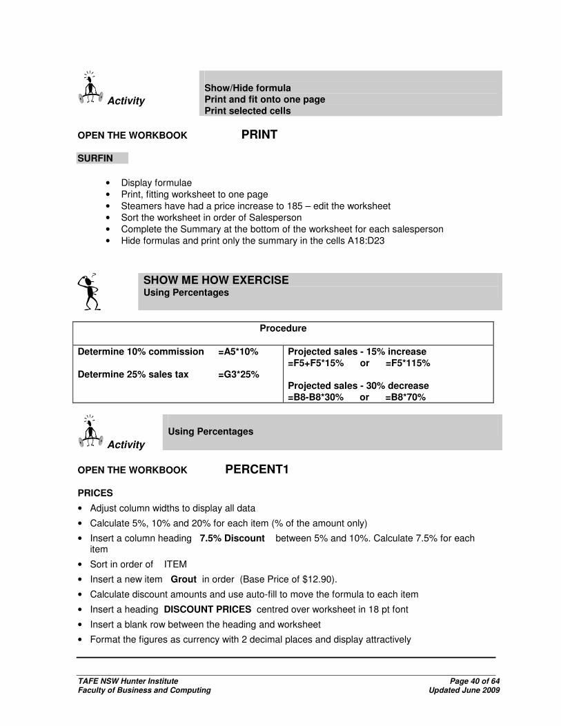
Show/Hide formula Print and fit onto one page Print selected cells
OPEN THE WORKBOOK PRINT SURFIN
• Display formulae • Print, fitting worksheet to one page • Steamers have had a price increase to 185 – edit the worksheet • Sort the worksheet in order of Salesperson • Complete the Summary at the bottom of the worksheet for each salesperson • Hide formulas and print only the summary in the cells A18:D23
SHOW ME HOW EXERCISE
Using Percentages
Procedure
Determine 10% commission =A5*10% Determine 25% sales tax =G3*25%
Projected sales - 15% increase =F5+F5*15% or =F5*115% Projected sales - 30% decrease =B8-B8*30% or =B8*70%
Activity
Using Percentages
OPEN THE WORKBOOK PERCENT1 PRICES
• Adjust column widths to display all data
• Calculate 5%, 10% and 20% for each item (% of the amount only)
• Insert a column heading 7.5% Discount between 5% and 10%. Calculate 7.5% for each item
• Sort in order of ITEM
• Insert a new item Grout in order (Base Price of $12.90).
• Calculate discount amounts and use auto-fill to move the formula to each item
• Insert a heading DISCOUNT PRICES centred over worksheet in 18 pt font
• Insert a blank row between the heading and worksheet
• Format the figures as currency with 2 decimal places and display attractively
TAFE NSW Hunter Institute Page 41 of 64 Faculty of Business and Computing Updated June 2009
COUNTRY
• Insert a row label TOTAL at bottom of worksheet and calculate Cost Price and Selling Price
• Insert a column heading TOTAL SALES and calculate the Total Sales of goods sold for month (Selling Price x Quantity Sold)
• Insert a new column heading called TOTAL COSTS between QUANTITY SOLD and TOTAL SALES and calculate (Cost Price x Quantity Sold)
• Insert a column heading called TOTAL GROSS PROFIT and calculate the Total Gross Profit for the month (Total Sales - Total Cost)
• Insert a new column label PROJECTED SALES - the premises are being renovated and total sales are expected to increase by 10% - insert a formula to determine future sales
• Wrap column headings in cell, vertically centred, using borders, colour and shading
• Format to currency where appropriate, print in landscape, vertically centred on page and displaying your name and filename
SHOW ME HOW EXERCISE
Create a basic chart on a separate sheet Add a title Change chart type
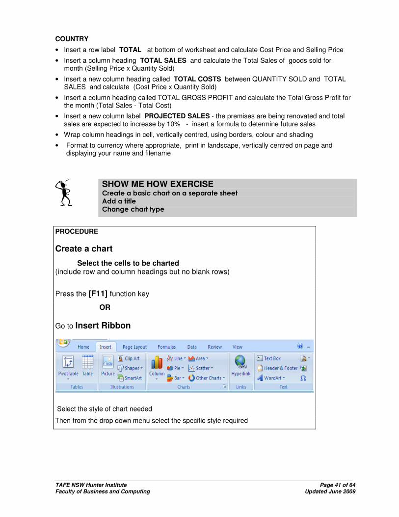
PROCEDURE
Create a chart
Select the cells to be charted (include row and column headings but no blank rows)
Press the [F11] function key
OR
Go to Insert Ribbon
Select the style of chart needed
Then from the drop down menu select the specific style required
TAFE NSW Hunter Institute Page 42 of 64 Faculty of Business and Computing Updated June 2009
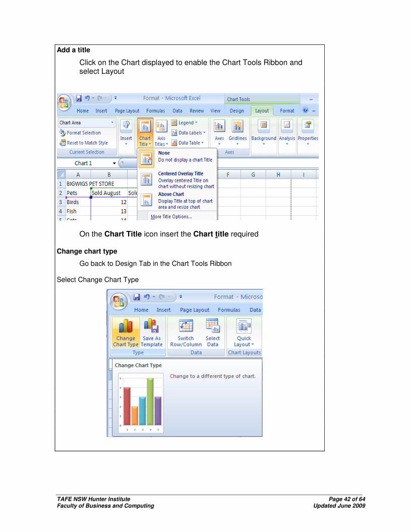
Add a title
Click on the Chart displayed to enable the Chart Tools Ribbon and select Layout
On the Chart Title icon insert the Chart title required
Change chart type
Go back to Design Tab in the Chart Tools Ribbon Select Change Chart Type
TAFE NSW Hunter Institute Page 43 of 64 Faculty of Business and Computing Updated June 2009
Activity
Create a basic chart Add a title Change chart type
OPEN THE WORKBOOK PRINT SURFIN
• Delete the blank row 19 (beneath the summary headings)
• Select the cells A18:C22 and press [F11] to create chart
• Add the title MAY SALES AND COMMISSION
• Change chart type to a Line chart
SHOW ME HOW EXERCISE
Absolute and Relative Cell References
RELATIVE REFERENCES When a formula is copied to another cell, the formula is automatically updated to the new location eg it adjusts as it is copied down - C1, C2, C3 etc ABSOLUTE REFERENCES An absolute cell address is indicated by a dollar sign ($) in front of the row or column label or both. Example a cell address $A$1 indicates that both the column and the row are absolute - that is the formula always refers back to the same cell. Formula can either be typed in, inserting the dollar signs manually or by pointing to the cell where reference is to be fixed and pressing <F4>
TAFE NSW Hunter Institute Page 44 of 64 Faculty of Business and Computing Updated June 2009
Activity
Absolute and Relative Cell References
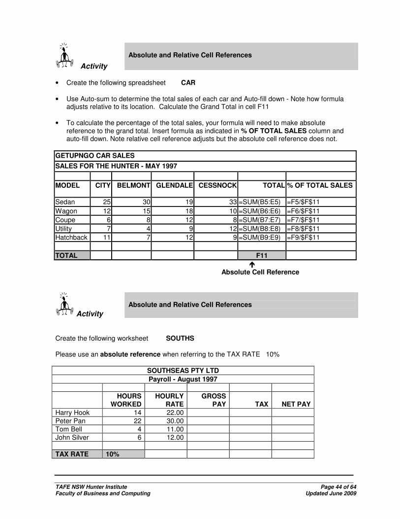
• Create the following spreadsheet CAR • Use Auto-sum to determine the total sales of each car and Auto-fill down - Note how formula
adjusts relative to its location. Calculate the Grand Total in cell F11 • To calculate the percentage of the total sales, your formula will need to make absolute
reference to the grand total. Insert formula as indicated in % OF TOTAL SALES column and auto-fill down. Note relative cell reference adjusts but the absolute cell reference does not.
GETUPNGO CAR SALES
SALES FOR THE HUNTER - MAY 1997
MODEL CITY BELMONT GLENDALE CESSNOCK TOTAL % OF TOTAL SALES
Sedan 25 30 19 33 =SUM(B5:E5) =F5/$F$11
Wagon 12 15 18 10 =SUM(B6:E6) =F6/$F$11
Coupe 6 8 12 8 =SUM(B7:E7) =F7/$F$11
Utility 7 4 9 12 =SUM(B8:E8) =F8/$F$11
Hatchback 11 7 12 9 =SUM(B9:E9) =F9/$F$11
TOTAL F11
� Absolute Cell Reference
Activity
Absolute and Relative Cell References
Create the following worksheet SOUTHS Please use an absolute reference when referring to the TAX RATE 10%
SOUTHSEAS PTY LTD
Payroll - August 1997
HOURS
WORKED HOURLY
RATE GROSS
PAY
TAX
NET PAY Harry Hook 14 22.00 Peter Pan 22 30.00 Tom Bell 4 11.00 John Silver 6 12.00
TAX RATE 10%

TAFE NSW Hunter Institute Page 45 of 64 Faculty of Business and Computing Updated June 2009
Create the following worksheet FINES Calculate the amount owing by each person - use an Absolute Reference for the Daily Overdue Rate
CARNABY VIDEO HIRE
Overdue Videos as at (current date)
DAILY OVERDUE RATE
$2.00
NAME
COMPUTER NUMBER
DAYS OVERDUE
AMOUNT OWING
ABLE 1890 4
COSSETINI 4367 1
CAMPBELL 2143 2
BARNES 1936 3
BEECH 2087 1

TAFE NSW Hunter Institute Page 46 of 64 Faculty of Business and Computing Updated June 2009
ASSESSMENT REVISION
OPEN THE WORKBOOK - REVISION - Click on FIXIT QUICK tab
• Insert a new column between Employee and Rate of Pay called HOURS WORKED and enter the following numbers/values: HOBAN, B – 40, LEWIS, G – 37, WILSON, W – 35, SMITH, B – 40, NEAL, Q – 37, MASON, R - 35
• Calculate GROSS PAY (Hours Worked x Rate of Pay)
• Insert a new column in Column E called TAX and calculate (Gross Pay * 25%)
• Insert a new column in Column F called NET PAY and calculate (Gross Pay - Tax)
• All employees have decided to pay superannuation - insert a new column between Gross Pay and Tax called SUPER - calculate superannuation (Gross Pay * 10%)
• Net Pay needs to be updated - edit formula to include full range of deductions
• Enter a new row label in Column A under employee’s names (leave one blank row) called TOTAL WAGES - calculate and insert total of NET PAY (Column G - use SUM function)
• Add another row under TOTAL WAGES called AVERAGE RATE and calculate average Rate of Pay
• Sort employees in descending order
• Insert a new employee in order PRATT, Katy Hours Worked (37) Rate of Pay ($12.60)
• Use Autofill to calculate Katy’s GROSS PAY, SUPER, TAX and NET PAY (start from original formula at top and copy down over existing numbers/values)
• Quentin Neal has left the company - delete him from the payroll
• Format the worksheet as follows: - Currency - Column labels should be all capitals, bold, text wrapped and vertically aligned in cell - Row labels should be in italics
• Insert a heading at top of worksheet FIXIT QUICK COMPANY centre it across worksheet and apply a border (top and bottom only)
• Insert a new row underneath the heading. Use =TODAY() function to insert date
• Insert a blank row between the date and column labels and apply a font colour to the column labels
• Increase the point size of the heading to 16 points
• Wendy Wilson has been attending a TAFE course - her hourly rate has been increased to $13.50 - edit data
• Create a header (filename) and footer (your name)
• Save changes to worksheet - Print two copies (one with formulae showing) in landscape, vertically centred on page
• Create a bar chart which displays the Workers’ names and their Net pays. Add an appropriate title.

TAFE NSW Hunter Institute Page 47 of 64 Faculty of Business and Computing Updated June 2009
Click on VINOS tab
• Calculate the GROSS PAY and Tax (Gross Pay * 25%) for all employees
• Insert a new row called OVERTIME between HOURS WORKED and GROSS PAY and insert
overtime hours as follows:
Wine, S (4) Scotch, D (6) Liquid, A (5)
Vino, B (9) Daniels, J (7)
• Edit GROSS PAY to include overtime ie RATE OF PAY * HOURS WORKED + OVERTIME *
RATE OF PAY * 2 - copy down formula to update
• Calculate amount for Net Pay and copy down
• Sort in ascending order of NAMES
• Bianca Vino’s brother Tony has joined the company - insert in order Rate of Pay (13.50)
Hours Worked (37) Overtime (1) - update Tony’s details by copying formula down again
• Insert a new row label TOTAL WAGES at A9 (14 pts, bold, wrap text and vertically align in
cell)
• Calculate total of GROSS PAY in B9 using range from Gross Pay
• Insert a new row label AVERAGE at A10 (14 pts, bold) and calculate the average Gross Pay
(using Gross Pay data) in cell B10
• Wrap text and vertically centre column labels and widen columns if ALL data is not displayed
Bold the row labels
• Add a border and pattern to the TOTAL WAGES and AVERAGE data
• Apply currency where appropriate (NOT THE HOURS WORKED PLEASE)
• Add a heading at the top of the worksheet VINO’S ESTATE - centre it across the worksheet
• Increase the point size for the heading to 18 and italicise
• Insert another row underneath the heading and insert the date =TODAY()
• Insert a blank row between the date and the rest of the worksheet
• Edit Amber Liquid’s hours worked - she lied - she only worked 22 hours
• Create a header (filename) and footer (your name in centre and date right aligned)
• Print a copy in landscape, vertically centred on page
• Graph the Name and Hours worked into a 3-D column chart. Add a suitable title.

TAFE NSW Hunter Institute Page 48 of 64 Faculty of Business and Computing Updated June 2009
Click on WORKERS tab
• This payroll has been prepared for the WORKERS ‘R US employees
• Insert a new column between Hourly Rate and Weekly Wage called HOURS WORKED and enter the following hours for each worker:
Dillon (37) Brendon (39) Kelly (35) Andria (37)
David (39) Steve (40) Donna (38)
• Calculate the WEEKLY WAGE and copy down
• Insert a new column after Weekly Wage called TAX - calculate Tax payable (Weekly Wage * 25%)
• Insert a new column after Tax called NET WAGE - calculate Net Wage
• Sort the worksheet in ascending order of Surname
• Insert a new row label TOTAL leaving a blank row between it and workers - calculate total amount of Weekly Wage, Tax and Net Wage
• Insert a new row label underneath Total called AVERAGE and calculate average hourly rate and hours worked
• Insert a heading WORKERS ‘R US at the top of the worksheet, increase point size to 16, bold and centre it across selection
• Insert a blank row between the heading and the worksheet
• Format the worksheet - use italics, bold, pattern and borders where it would highlight data. Vertically centre and wrap column labels in box - format to currency where appropriate - increase row heights slightly and column widths to display all data
• There have been some changes, amend as follows:
⇒ Brendon Walsh has left - delete his record
⇒ Melissa Nevins has joined the company, insert her details in correct order - she worked 15 hours this week at an hourly rate of $16.70 - ensure you check your formula and/or range to see if all workers are included in totals etc.
⇒ Donna Martin’s hourly rate has increased to $15.30 - amend her record
• Save the worksheet under a new name WORKERS1 - double click WORKERS tab at bottom of workbook and type new name in dialog box.
• Print a copy of your worksheet in landscape, centred vertically on the page with filename included in the Header and your name in the Footer.
• Create a column chart as a separate sheet showing Workers and their Hourly Rates. Print a copy.
TAFE NSW Hunter Institute Page 49 of 64 Faculty of Business and Computing Updated June 2009
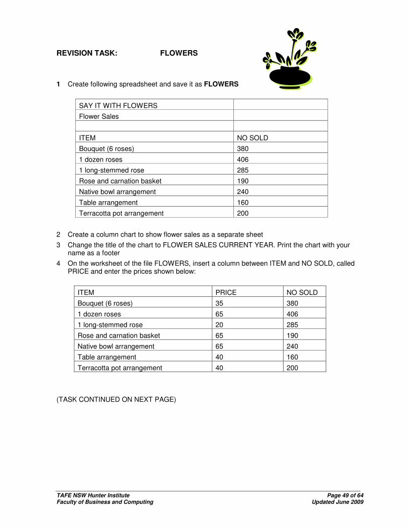
REVISION TASK: FLOWERS
1 Create following spreadsheet and save it as FLOWERS
SAY IT WITH FLOWERS
Flower Sales
ITEM NO SOLD
Bouquet (6 roses) 380
1 dozen roses 406
1 long-stemmed rose 285
Rose and carnation basket 190
Native bowl arrangement 240
Table arrangement 160
Terracotta pot arrangement 200
2 Create a column chart to show flower sales as a separate sheet
3 Change the title of the chart to FLOWER SALES CURRENT YEAR. Print the chart with your name as a footer
4 On the worksheet of the file FLOWERS, insert a column between ITEM and NO SOLD, called PRICE and enter the prices shown below:
ITEM PRICE NO SOLD
Bouquet (6 roses) 35 380
1 dozen roses 65 406
1 long-stemmed rose 20 285
Rose and carnation basket 65 190
Native bowl arrangement 65 240
Table arrangement 40 160
Terracotta pot arrangement 40 200
(TASK CONTINUED ON NEXT PAGE)

TAFE NSW Hunter Institute Page 50 of 64 Faculty of Business and Computing Updated June 2009
5 Insert two more columns to the left of column C, as follows:
ITEM PRICE LESS DISCOUNT
SELLING PRICE
NO SOLD
Bouquet (6 roses) 35 380
1 dozen roses 65 406
1 long-stemmed rose 20 285
Rose and carnation basket
65 190
Native bowl arrangement 65 240
Table arrangement 40 160
Terracotta pot arrangement
40 200
6 Insert formula in Cell C5 to calculate the discount amount – it is 5% of the Price. Fill down to calculate discount on all flower prices
7 To calculate the selling price, enter a formula in D5, subtracting the discount amount from the Price. Fill down
8 Enter a new column heading in F4: TOTAL
9 In F5, enter a formula to multiply the number of items sold by the selling price. Fill down
10 In A13, enter the heading: TOTAL SALES
11 Enter a formula in E13 and F13 to calculate both the total number sold and the total sales amount
12 In cell A14, enter the heading: AVERAGE SALES and enter a formula in F14 to calculate the average figure in the cell range F5:F11
13 Sort the spreadsheet so that the least expensive item is at the beginning of the list
14 Format the spreadsheet using borders, wrap text and apply bold, italics and currency where appropriate
15 Change vertical alignment of text in cells to centre, where necessary
16 Centre the worksheet on the page and add your name as a footer and the filename and date as a header
17 Change the page orientation to landscape
18 Print the worksheet, displaying the formula and making sure that it fits on one page
19 Ask your teacher to check your work

TAFE NSW Hunter Institute Page 51 of 64 Faculty of Business and Computing Updated June 2009
If you have checked your results with your trainer and have successfully completed the revision work, you should now be ready to attempt the summative assessment task for this Unit. Please ask your trainer for
the assessment.

TAFE NSW Hunter Institute Page 52 of 64 Faculty of Business and Computing Updated June 2009
Microsoft Excel
Spreadsheets
Extra Tips

TAFE NSW Hunter Institute Page 53 of 64 Faculty of Business and Computing Updated June 2009
MICROSOFT EXCEL – QUICK REFERENCE GUIDE
Function How is it done? Bold
Highlight and click on Borders, remove Highlight area and click on
Borders, add Highlight area and click on
Centre Align Highlight and click on
Centre (on page for printing)
Page Layout Ribbon Page Setup selection button
Column Width, resize
Highlight entire column(s) and resize using
Copy Highlight and click on
Currency, apply Highlight and click on
Cut
Highlight and click on Drag and drop text Highlight cells then move using
Fit (on one page for printing)
Page Layout Ribbon
Page Setup selection button Font, change size Highlight cell and click on in Home Ribbon
Font, change style Highlight cell and click on in Home Ribbon
Font, change colour Highlight cell and click on then select colour in Home Ribbon
Footers Insert Ribbon/Header/Footer
Gridlines (print showing)
Page Layout Ribbon, Sheet Options
Headers
Insert Ribbon /Header/Footer Headers, automatic date Headers, automatic page number Headers, automatic workbook name Headers, automatic worksheet name
Header Footer Tools Design Tab
TAFE NSW Hunter Institute Page 54 of 64 Faculty of Business and Computing Updated June 2009
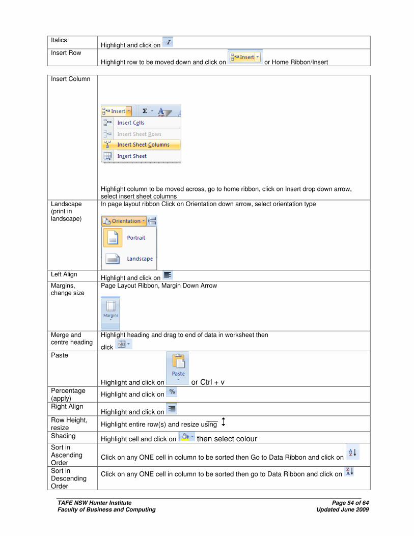
Italics Highlight and click on
Insert Row
Highlight row to be moved down and click on or Home Ribbon/Insert
Insert Column
Highlight column to be moved across, go to home ribbon, click on Insert drop down arrow, select insert sheet columns
Landscape (print in landscape)
In page layout ribbon Click on Orientation down arrow, select orientation type
Left Align
Highlight and click on Margins, change size
Page Layout Ribbon, Margin Down Arrow
Merge and centre heading
Highlight heading and drag to end of data in worksheet then
click
Paste
Highlight and click on or Ctrl + v Percentage (apply)
Highlight and click on
Right Align Highlight and click on
Row Height, resize
Highlight entire row(s) and resize using
Shading Highlight cell and click on then select colour Sort in Ascending Order
Click on any ONE cell in column to be sorted then Go to Data Ribbon and click on
Sort in Descending Order
Click on any ONE cell in column to be sorted then go to Data Ribbon and click on

TAFE NSW Hunter Institute Page 55 of 64 Faculty of Business and Computing Updated June 2009
Spellcheck
Click on Review Ribbon then click on Underline, double
Format/Cells/Font/Underline:
Underscore Highlight and click on
Wrap Text Home Ribbon Click on
EXAMPLES OF SIMPLE FORMULAS
All formulas (except Autosum) must start with an = sign.
Total
Autosum – adds a list of numbers to the left or above
Addition =SUM(B2:B10) =B2+B10
Adds ALL the cells from B2 to B10 Adds contents of B2 to contents of B10
Subtraction =B10-B2
Subtracts cell B2 from cell B10
Multiplication =B2*B10
Multiplies cell B2 by cell B10
Division =B2/B10 Divides cell B2 by cell B10
Average =AVERAGE(B2:B10) Finds the average of cells B2 to B10
Maximum =MAX(B2:B10) Finds the highest value in cells B2 to B10
Minimum =MIN(B2:B10) Finds the lowest value in cells B2 to B10
Percentage
=B2*10% =B2+B2*10% =B2-B2*10%
Finds 10% of the value in cell B2 Finds the new value including 10% markup Finds the new value deducting 10% markdown
Today =TODAY() This shows the system date
Turn Formulas on/off
CTRL ~ This displays the formulas in your worksheet, press again to return to your data

TAFE NSW Hunter Institute Page 56 of 64 Faculty of Business and Computing Updated June 2009
Microsoft Excel (Spreadsheets)Microsoft Excel (Spreadsheets)Microsoft Excel (Spreadsheets)Microsoft Excel (Spreadsheets) Formatting and FormulaeFormatting and FormulaeFormatting and FormulaeFormatting and Formulae
Formatting Hints
� To apply currency spaced away from numbers with two decimal places.
Highlight the data to be changed – click on .
� To apply currency next to numbers with choice of decimal places.
Highlight the data to be changed – click on Format/Cells/Number/Currency and select your
choices.
� To prepare a spreadsheet for printing:
Go to File/Page Setup – click through all Tabs – change orientation if necessary, apply vertical and horizontal centring, add header/footer.
� To Wrap Text in a Cell
Highlight the cell or cells to be wrapped – click on Format/Cells/Alignment/Wrap Text.
If the text doesn’t wrap – you may need to make your cell narrower so the words wrap. Sometimes, you will also need to make your cell deeper to see the wrapped text.
� To Vertically Align Data in a Cell (equal space above and below information)
Highlight the cell or cells to be vertically aligned – click on Format/Cells/Alignment/Text Alignment/Vertical – change to Center.
To resize a column – position your cursor to the right of the column letter (eg A) to be resized and when the double headed arrow appears – click and drag to desired width. To resize a row – position your cursor below the row number (eg 1) to be resized and when the double headed arrow appears – click and drag to desired depth.
To resize multiple columns – highlight all the columns to be changed then position your cursor between any two columns (eg B and C) and when the double headed arrow appears – click and drag to desired width. This will make all the highlighted columns the same.
To resize multiple rows – highlight all the rows to be changed then position your cursor between any two rows (eg 1 and 2) and when the double headed arrow appears – click and drag to desired height. This will make all the highlighted rows the same.
To centre heading across worksheet – highlight the heading to be centered (with the fat cross) and drag across to the last column containing information in the worksheet.
Click on the merge and center button . To cancel merge – go to Format/Cells/Alignment and remove tick from Merge cells.
TAFE NSW Hunter Institute Page 57 of 64 Faculty of Business and Computing Updated June 2009
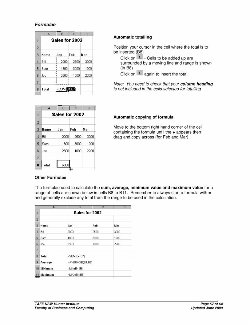
Formulae
Other Formulae
The formulae used to calculate the sum, average, minimum value and maximum value for a range of cells are shown below in cells B8 to B11. Remember to always start a formula with = and generally exclude any total from the range to be used in the calculation.
Automatic totalling
Position your cursor in the cell where the total is to be inserted (B8)
Click on - Cells to be added up are surrounded by a moving line and range is shown (in B8)
Click on again to insert the total
Note: You need to check that your column heading is not included in the cells selected for totalling
Automatic copying of formula
Move to the bottom right hand corner of the cell containing the formula until the + appears then drag and copy across (for Feb and Mar).
TAFE NSW Hunter Institute Page 58 of 64 Faculty of Business and Computing Updated June 2009
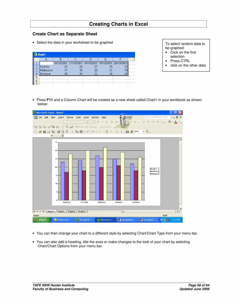
Creating Charts in Excel
Create Chart as Separate Sheet
• Select the data in your worksheet to be graphed
• Press F11 and a Column Chart will be created as a new sheet called Chart1 in your workbook as shown
below:
• You can then change your chart to a different style by selecting Chart/Chart Type from your menu bar. • You can also add a heading, title the axes or make changes to the look of your chart by selecting
Chart/Chart Options from your menu bar.
To select random data to be graphed: • Click on the first
selection • Press CTRL • click on the other data

TAFE NSW Hunter Institute Page 59 of 64 Faculty of Business and Computing Updated June 2009
Create Chart as an Object in your Worksheet • Select the data in your worksheet to be graphed
• Click on the Chart Wizard Button and: • Select the type of chart you would like and press NEXT • Check the data shown on the chart and press NEXT • Enter a title for your chart and the axes if required, then press NEXT • Check the chart is going to be placed as an object in your sheet as shown below
Your chart will appear in the same worksheet as your data as shown below: • Click on it and you can resize it using the handles on the outside • To change font sizes, etc – RIGHT MOUSE CLICK on the area to be changed
0
5
10
15
20
25
30
35
16/1
0/20
01
17/1
0/20
01
18/1
0/20
01
19/1
0/20
01
20/1
0/20
01
Sydney
Melbourne
Brisbane

TAFE NSW Hunter Institute Page 60 of 64 Faculty of Business and Computing Updated June 2009
EXAMPLE SHOWING DISCOUNT AND DISCOUNTED PRICE
A B C D E
1 Item Price Discount % Amount of Discount
Discounted Price
2
3 Dress $60.00 10% =B3*C3 =B3-(B3*C3)
4 Jacket $120.00 10% =B4*C4 =B4-(B4*C4)
5
Answers as below:
A B C D E
1 Item Price Discount % Amount of Discount
Discounted Price
2
3 Dress $60.00 10% 6 54
4 Jacket $120.00 10% 12 108
5
EXAMPLE SHOWING GST AND INCREASED PRICE
A B C D E
1 Item Price GST % Amount of GST
New Price
2
3 Pants $50.00 10% =B3*C3 =B3+(B3*C3)
4 Skirt $80.00 10% =B4*C4 =B4+(B4*C4)
5
Answers as below:
A B C D E
1 Item Price GST % Amount of GST
New Price
2
3 Pants $50.00 10% 5 55
4 Skirt $80.00 10% 8 88
5
Top Related