


Languages
Pages
Legal

CRANK-NICOLSON SCHEME FOR ASIAN OPTION
By
LEE TSE YUENG
A thesis submitted to the Department of Mathematical and Actuarial Sciences,
Faculty of Engineering and Science,
Universiti Tunku Abdul Rahman,
in partial fulfillment of the requirements for the degree of
Master of Science
August 2012

TABLE OF CONTENTS
Page
ABSTRACT ii
ACKNOWLEDGEMENTS iv
SUBMISSION OF THESIS v
APPROVAL SHEET vi
DECLARATION vii
LIST OF TABLES viii
LIST OF FIGURES ix
LIST OF ABBREVIATIONS/NOTATION/GLOSSARY OF TERMS x
CHAPTER
1.0 INTRODUCTION 1
1.1 Stock Price Model 1
1.2 Mechanics of Option 4
1.3 Styles of Option 7
2.0 REVIEW ON PROBABILITY THEORY 11
3.0 EUROPEAN OPTION 17
3.1 Introduction 17
3.2 Itô's Lemma Approach to Black-Scholes Equation 24
3.3 Crank-Nicolson Finite Difference Method 28
3.4 Implementation 30
3.5 Stability Analysis 32
3.6 Simulation and Analysis 35
3.7 Conclusion 38
4.0 ASIAN OPTION - A TWO-DIMENSIONAL PDE 39
4.1 Introduction 39
4.2 Partial Differential Equation for Asian option 40
4.3 Method of Solution 43
4.4 Boundary Values 43
4.5 Discretization 45
4.6 Implementation 49
4.7 Stability Analysis 51
4.8 Simulation and Analysis 55
4.9 Conclusion 58
5.0 ASIAN OPTION - A ONE-DIMENSIONAL PDE 59
5.1 Introduction 59
5.2 Change of Numéraire Argument 59
5.3 Boundary Values 64
5.4 Partial Differential Equation for Asian option 65
5.5 Discretization 66
5.6 Simulation and Analysis 67
5.7 Conclusion 69
6.0 CONCLUSION 70
REFERENCES 72
APPENDICES 76
ii
ABSTRACT
CRANK-NICOLSON SCHEME FOR ASIAN OPTION
Lee Tse Yueng
Finite difference scheme has been widely used in financial mathematics. In
particular, the Black-Scholes option pricing model can be transformed into a
partial differential equation and numerical solution for option pricing can be
approximated using the Crank-Nicolson difference scheme. This approach
provides a stable scheme under different volatility condition. Besides, it allows
us to acquire the option value at different times, including time zero in a single
iteration.
The thesis begins with a brief introduction to option pricing and a review on
probability theory in Chapter 1 and 2, followed by a summary of some basic
ideas and techniques for option of European style in Chapter 3. Chapter 4 and
5 contain the main results of this thesis and Chapter 6 is the conclusion.
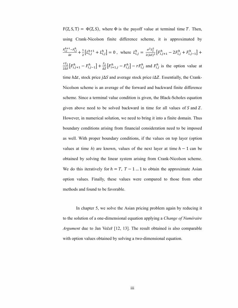
In Chapter 4, we obtain the value of Asian option by solving a two-
dimensional Black-Scholes equation using a simple Crank-Nicolson finite
difference scheme. If is the stock price and is the average stock price at
time , then the Black-Scholes equation for the Asian option price FZ, S, t is
given by F
rS F
S σS
F
S Z
F
Z rF 0 with terminal value
iii
FZ, S, T ΦZ, S, where Φ is the payoff value at terminal time . Then,
using Crank-Nicolson finite difference scheme, it is approximated by
, !,
∆# $
%&',(
)*$ &',() + 0 , where &',(
) ,-
∆- %.',(*$) 2.',(
) .',(!$) +
0-
∆-%.',(*$
) .',(!$) +
-
∆1%.'*$,(
) .',() + 2.',(
) and .',() is the option value at
time 3∆, stock price 4∆ and average stock price 5∆. Essentially, the Crank-
Nicolson scheme is an average of the forward and backward finite difference
scheme. Since a terminal value condition is given, the Black-Scholes equation
given above need to be solved backward in time for all values of and .
However, in numerical solution, we need to bring it into a finite domain. Thus
boundary conditions arising from financial consideration need to be imposed
as well. With proper boundary conditions, if the values on top layer (option
values at time h) are known, values of the next layer at time 3 1 can be
obtained by solving the linear system arising from Crank-Nicolson scheme.
We do this iteratively for 3 , 1 … 1 to obtain the approximate Asian
option values. Finally, these values were compared to those from other
methods and found to be favorable.
In chapter 5, we solve the Asian pricing problem again by reducing it
to the solution of a one-dimensional equation applying a Change of Numéraire
Argument due to Jan Večeř [12, 13]. The result obtained is also comparable
with option values obtained by solving a two-dimensional equation.

iv
ACKNOWLEDGEMENT
First and foremost, I would like to express my utmost deep and sincere
gratitude to my supervisor, Dr Chin Seong Tah. He has guided me in learning
financial mathematics from the very beginning. His personal guidance with
wide knowledge and words has given me a great value. I am also thankful for
his time, patience and understanding for everything, especially during my
difficult moments.
Thanks to Dr. Goh Yong Kheng, Head of Department of Mathematical
Sciences and Actuarial Sciences, who gave me the encouragement and support
to begin my Master’s programme.
My sincere thanks also go to Ruenn Huah Lee, for his untiring help, valuable
advice and support, not only my research, and during my difficult moment as
well. I was very lucky to have such a best friend.
I owe my loving thanks to my family. Thanks for their understanding,
encouragement and loving support throughout my life.
Lastly, I would like to offer my regards and blessings to all of those who
supported me during the completion of this thesis.
Again, thank you very much to all of you.

v
FACULTY OF ENGINEERING AND SCIENCES
UNIVERSITI TUNKU ABDUL RAHMAN
Date : 08th August 2012
SUBMISSION OF THESIS
It is hereby certified that _ LEE TSE YUENG__ ( ID No: _09UIM02242 )
has completed this thesis entitled “CRANK-NICOLSON SCHEME FOR
ASIAN OPTION” under the supervision of DR CHIN SEONG TAH
(Supervisor) from the Department of Mathematical and Actuarial Sciences,
Faculty of Engineering and Science.
I understand that the University will upload softcopy of my thesis in pdf
format into UTAR Institutional Repository, which may be made accessible to
UTAR community and public.
Yours truly,
___________________
( LEE TSE YUENG )

vi
APPROVAL SHEET
This thesis entitled “CRANK-NICOLSON SCHEME FOR ASIAN
OPTION” was prepared by LEE TSE YUENG and submitted as partial
fulfillment of the requirements for the degree of Master of Mathematical
Sciences at Universiti Tunku Abdul Rahman.
Approved by:
___________________________
(Dr. Chin Seong Tah) Date:…………………..
Professor/Supervisor
Department of Mathematical and Actuarial Sciences
Faculty of Engineering and Science
Universiti Tunku Abdul Rahman

vii
DECLARATION
I, Lee Tse Yueng hereby declare that the thesis is based on my original work
except for quotations and citations which have been duly acknowledged. I also
declare that it has not been previously or concurrently submitted for any other
degree at UTAR or other institutions.
_______________________
( LEE TSE YUENG )
Date : _______________________

viii
LIST OF TABLES
Table
1.1
Call option
Page
5
1.2 Put option
6
3.1
4.1
5.1
5.2
Comparison of Crank-Nicolson scheme and Black-
Scholes formula for pricing European call option
with k = 20 and T = 1, where T is in year.
Comparison of Crank-Nicolson finite difference
scheme and simulation method for pricing the
Asian call option with K = 20 and Tmax = 1, where
Tmax is in year.
Comparison of Crank-Nicolson finite difference
scheme and CRR Binomial Tree for pricing the
Asian call option with K = 20 and Tmax = 1, where
Tmax is in year.
Comparison of Asian call option value by solving
one-dimensional and two-dimensional partial
difference equation(PDE) using Crank-Nicolson
scheme with K = 20 and Tmax = 1, where Tmax is
in year.
36
56
68
69
ix
LIST OF FIGURES
Figures
1.1
KLSE raw data plot
Page
1
1.2 Return series, log
2
1.3
1.4
1.5
3.1
3.2
3.3
4.1
4.2
4.3
4.4
Histogram plot of return series
Payoff of call option at time
Payoff of put option at time
Comparison of Crank-Nicolson finite difference
scheme and simulation method for pricing the
European call option with 20 , 0.1 ,
0.35 and 1, where is in year.
A three-dimensional plot of European call option
with 20 , 0.1 , 0.35 , and 1 ,
where is in year.
A three-dimensional plot of European call option
with 50 , 0.1 , 0.35 , and 1 ,
where is in year.
A three-dimensional grid
Relationship between values of at several points
Comparison of Crank-Nicolson finite difference
scheme and simulation method for pricing the
Asian call option under different stock price with
20, 0.1, 0.25, and 1, where is in year.
A three-dimensional plot of Asian call option with
20, 0.1, 0.25, at time zero.
2
6
7
36
37
38
46
48
57
58

x
LIST OF ABBREVIATIONS
KLSE CI Kuala Lumpur Stock Exchange Composite Index
PDE Partial Differential Equation
SDE Stochastic Differential Equation

CHAPTER 1
INTRODUCTION
1.1 Stock Price Model
Stock prices fluctuate widely in reaction to new information. Since market
participants compete to be the first to profit from new information, as a result,
all these information are immediately reflected in current price of the stock
market. Hence, successive price changes are not correlated and the movement
is unpredictable, since they depend on as-yet unrevealed information. However,
we can obtain the expected size of the prices by using statistical method.
As an example, consider the KLSE CI (Kuala Lumpur Stock Exchange
Composite Index) daily closing values from January 2, 2004, to February 15,
2008, for a total of 1020 data.
Figure 1.1: KLSE raw data plot
2
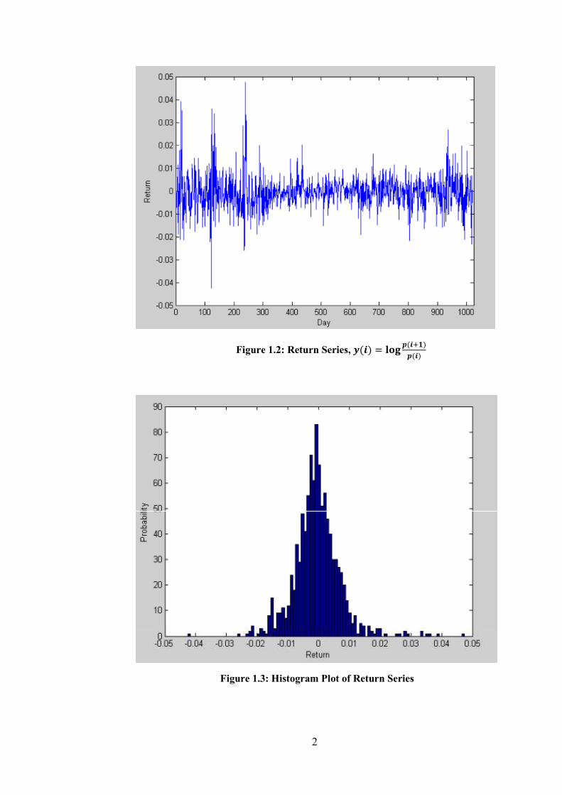
Figure 1.2: Return Series, () = ()()
Figure 1.3: Histogram Plot of Return Series
3
A typical size of the fluctuations, about half of a percent can be
identified in this example. The histogram plot above (figure 1.3) indicates that
the fluctuations of stock price are uncorrelated and have mean near zero. This
typical size is one of the most important statistical quantity that we can extract
from the market price history. We may be curious about the form of this
distribution, for instance, if it is a normal distribution.
From the shape of the histogram plot in figure 1.3, it is very plausible
that stock prices are lognormally distributed. This simply means that there are
constants and such that the logarithm of return, is normally distributed
with mean and variance . Symbolically,
ℙ ∈ , = ℙ log !" ∈ log , log
= 1√2' ( exp ,− (. − )2 /012 3012 4 5..
This is so if we assume stock prices evolve according to
7 = exp 8,9 − 2 / : + <7=
= exp( + <7) where
= ,9 − 2 / :
and <7 is the standard ℙ - Brownian motion.
4
1.2 Mechanics of Option
As stock prices fluctuate widely, market participants need to hedge
against their risks. Derivatives provide a rich means for hedging. Derivatives
are assets whose values are derived from the value of underlying assets’ prices
[1]. Option is a type of derivative. It is a contract. An option gives the holder
the right, but not the obligation, to choose whether to execute the final
transaction or not. There are two basic types of option, the call option and the
put option. A call option gives the holder the right, but not the obligation to
buy an underlying stock at time > with strike price ?, while a put option gives
the holder the right (again, not the obligation) to sell an underlying stock at
time > with price ?. In fact, the terms call and put refer to buying and selling
respectively. These are financial terms [2].
A call option will be exercised if the market price of the asset at the
expiration time, is greater than the strike price, ? that is,
> ?
This kind of option is said to be in the money because an asset worth can be
purchased for only ?.
On the other hand, if the strike price is less than at the expiration
time, that is,
< ?
Then, the call option will not be exercised because we can purchase the asset
with cheaper price at open market. Thus, the option will be worthless and is
said to be out of the money.
5
For put option, all aforesaid conditions are reversed. If the strike price
of the asset is less than the market price of the asset at the expiration time,
namely,
> ?
Then, the put option will not be exercised and is said to be out of the money.
The seller can sell the asset to the open market with the market price, which is
higher than the price stated in the put option.
The put option will only be exercised when the actual price (market
price) of the asset is less than the strike price of the asset at expiration time,
that is
< ?
In this situation, the put option is said to be in the money.
Regardless of call option or put option, an option is said to be at the
money (or on the money) if and only if the market price of the asset at the
expiration time, is equal to the strike price ?.
= ?
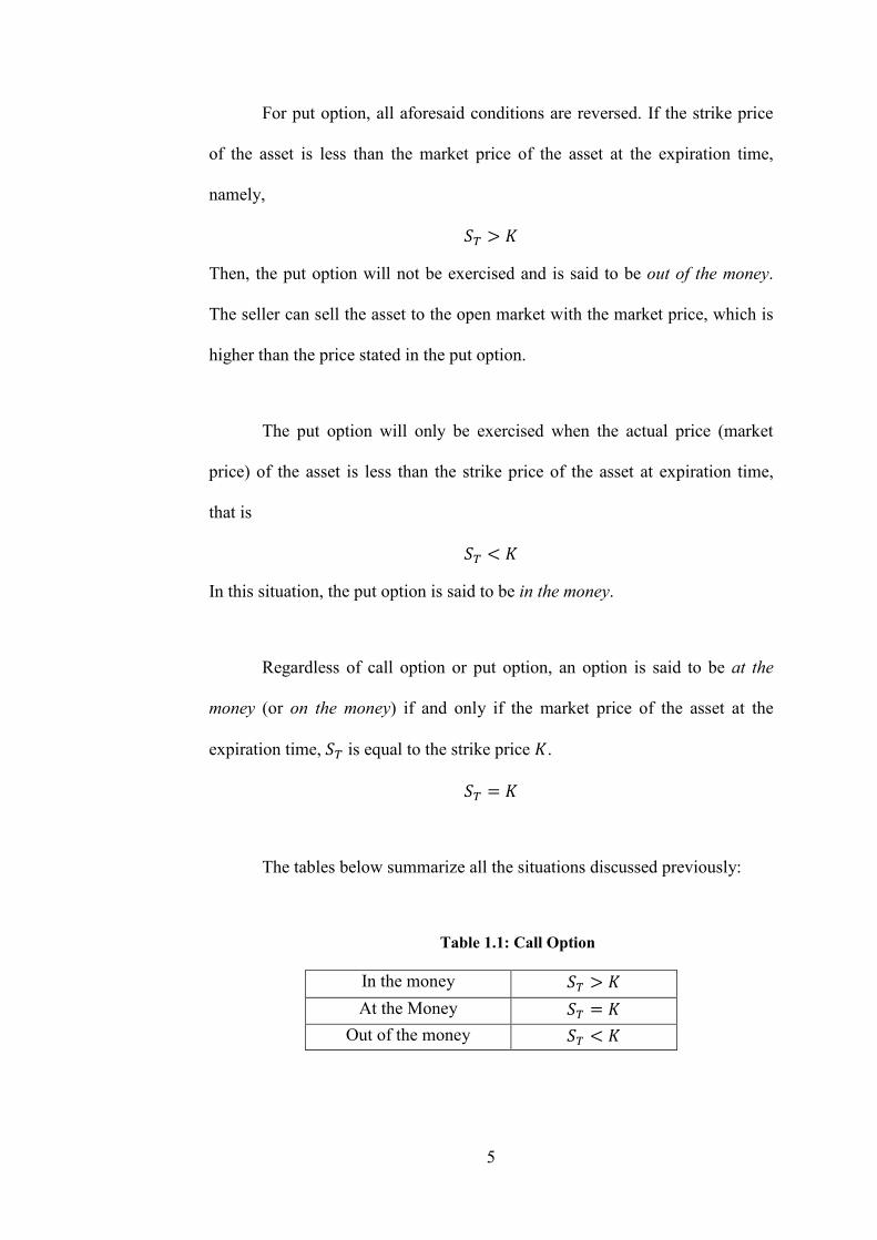
The tables below summarize all the situations discussed previously:
Table 1.1: Call Option
In the money > ?
At the Money = ?
Out of the money < ?

6
Table 1.2: Put Option
In the money < ?
At the Money = ?
Out of the money > ?
The payoff of call option and put option at time > may be written
respectively as below:
B(>) = ( − ?)
= maxE( − ?), 0G
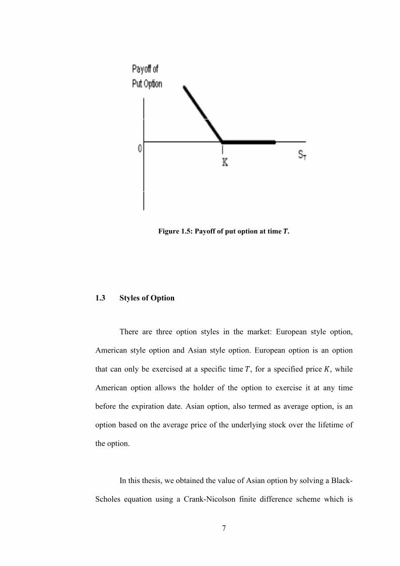
H(>) = (? − )
= maxE(? − ), 0G
These functions can be represented graphically as the following:
Figure 1.4: Payoff of call option at time I.
7
Figure 1.5: Payoff of put option at time I.
1.3 Styles of Option
There are three option styles in the market: European style option,
American style option and Asian style option. European option is an option
that can only be exercised at a specific time >, for a specified price ?, while
American option allows the holder of the option to exercise it at any time
before the expiration date. Asian option, also termed as average option, is an
option based on the average price of the underlying stock over the lifetime of
the option.
In this thesis, we obtained the value of Asian option by solving a Black-
Scholes equation using a Crank-Nicolson finite difference scheme which is

8
stable and easy to program. The Asian option prices so obtained compare
favorably with those form simulation method.
In general, the study of Asian option pricing can be divided into three
classes: close form solution for the Laplace transform, Monte Carlo simulation
and finite difference method for partial differential equation.
Apart from a closed-form formula for a Laplace transform of the Asian
option price obtained by H. Geman and M. Yor [4], the price of Asian option is
not known in explicit closed form. M. Fu, D. Madan and T. Wang [5]
compares Monte Carlo and Laplace transform methods for Asian option
pricing. Besides, the theory of Laplace transform is extended by deriving the
double Laplace transform of the continuous arithmetic Asian option [4]. V.
Linetsky [6] derives a new integral formula for the price of continuously
sampled Asian option, but for the cases of low volatility, it converges slowly.
Monte Carlo simulation [7,8,9] and finite difference method for partial
differential equation (PDE) [10,11,12,13,14] are the two main numerical
method to price the Asian options. However, without the enhancement of
variance reduction techniques, Monte Carlo simulation can be computationally
expensive and one must also resolves the inherent discretization bias resulting
from the approximation of continuous time processes through discrete
sampling as shown by Broadie, Glasserman and Kou [15].
In principle, one can find the price of an Asian option by solving a
partial differential equation in two space dimensions [16]. Besides, Ingersoll

9
found that the two-dimensional PDE for a floating strike Asian option can be
reduced to a one-dimensional PDE[16]. In 1995, Rogers and Shi formulated a
one-dimensional PDE which is able to model both floating and fixed strike
Asian options [10]. However, since the diffusion term is very small for values
of interest on the finite difference grid, it is very hard to solve this PDE
numerically. Andreasen applied Rogers and Shi’s reduction to discretely
sampled Asian option[17]. Večeř J. develops the change of JKLMOPOM
techniques for pricing Asian options. This technique was extended to jump
process by Večeř and Xu [13,14].
In 2001, Kwok, Wong and Lau discussed about the explicit scheme for
multivariate option pricing [18]. They found that the correlations among
underlying variables deteriorate the accuracy of the computation. Besides, the
explicit scheme is very difficult to control the stability in general.
However, these problems can be solved through our works here as PDE
governing the value of Asian option with no correlation term. So, the first
problem can be eliminated. The von Neumann stability analysis also carries out
to ensure our result is stable [19].
Although there are a lot of ways to compute the value of Asian option,
the Crank-Nicolson scheme is the only method that can be easily generalized to
cope with early exercise decision for an Asian option by comparing the
computed option value and immediate exercise value at each node backward in
time. Hence, this method can be applied to options without Asian feature, or
extended to American style Asian option. Besides, our proposed method is

10
unconditionally stable compared to other methods, for instance, CRR binomial
model. The CRR binomial model is only conditional stable of the type
∆: ∽ ∆.. Besides, a forward shooting grid (FSG) approach is required in this
CRR model as it cannot record the realized averaged value in almost all Asian
options. However, the FSG version of CRR model contains a subtle bias. [20].
11
CHAPTER 2
REVIEW OF PROBABILITY THEORY
Let us begin by recalling some of the definitions and basic concepts of
elementary probability. A probability space is a triple (Ω, ℱ, ℙ) where Ω is
the set of sample space, ℱ is a collection of subsets of Ω, events, and ℙ is
the probability measure defined for each event U ∈ ℱ. The collection ℱ is a
-field or -algebra, namely, Ω ∈ ℱ and ℱ is closed under the operations
of countable union and taking complements. The probability measure ℙ
must satisfy the usual axioms of probability [1,3]:
• 0 ≤ ℙU ≤ 1, for all U ∈ ℱ,
• ℙΩ = 1
• ℙA ∪ B = ℙA + ℙB for any disjoint U, Z ∈ ℱ, • If U[ ∈ ℱ for all J ∈ ℕ and U] ⊆ U ⊆ ⋯ then ℙU[ ↑ ℙ⋃[U[ as J ↑ ∞.
Definition 2.1. A real-valued random variable, b , is a real-valued
function on Ω that is ℱ -measurable. In the case of discrete random variable
(that is a random variable that can only take on countable many distinct values)
this simply means
Ec ∈ Ω: X(c) = xG ∈ ℱ
so that ℙ assigns a probability to the event EX = xG. For a general real-valued
random variable we require that
Ec ∈ Ω: X(c) ≤ xG ∈ ℱ
so that we can define the distribution function, f(.) = ℙb ≤ ..
12
To specify a (discrete time) stochastic process, we require not just a single σ-
field ℱ, but an increasing family of them.
Definition 2.2. Let ℱ be a σ-field. We call EℱgGgh a filtration if
1. ℱg is a sub-σ-algebra of ℱ for all :. 2. ℱk ⊆ ℱg for s < :.
The quadruple (Ω, ℱ, EℱgGgh, ℙ) is called a filtered probability space.
We are primarily concerned with the natural filtration, Eℱ7mG7h , associated
with a stochastic process Eb7G7h. Let ℱ7m encodes the information generated
by the stochastic process b on the interval 0, :. That is U ∈ ℱ 7m if, based
upon observations of the trajectory Eb7G7h, it is possible to decide whether or
not U has occurred.
Definition 2.3. A real-valued stochastic process is a family of real-
valued function Eb7G7h on Ω . We say that it is adapted to the filtration
Eℱ7G7h if b7 is ℱ7 measurable for each :.
One can then think of the σ-field ℱ7 as encoding all the information about
the evolution of the stochastic process up until time :, that is, if we know
whether each event in ℱ7 happens or not then we can infer the path followed by
the stochastic process up until time :. We shall call the filtration that encodes
precisely this information the natural filtration associated to the stochastic
process Eb7G7h.
13
Notation: If the value of a stochastic variable n can be completely determined
given observations of the trajectory Eb7Gopo7 then we write n ∈ ℱ 7m . More
than one process can be measurable with respect to the same filtration.
Definition 2.4. If EYgGgh is a stochastic process such that we have
Y ∈ ℱ gr for all t ≥ 0 , then we say that EYgGgh is adapted to the filtration
EℱgrGgh.
Definition 2.5. Suppose that b is an ℱ -measurable random variable
with u|b| < ∞ . Suppose that w ⊆ ℱ is a -field; then the conditional
expectation of b given x, written uyb|w, is the w-measurable random variable
with the property that for any U ∈ w
uzyb|w; U| ≜ ( uyb|w5ℙ =~ ( b5ℙ~ ≜ ub; U The conditional expectation exists, but is only unique up to the addition of a
random variable that is zero with probability one.
The tower property of conditional expectations:
Suppose that ℱ ⊆ ℱ; then
uzyuzyb|ℱ|ℱ| = uyb|ℱ
Taking out what is known in conditional expectations:
Suppose that ub and ub < ∞, if is ℱ[-measurable, we have
uyb|ℱ[ = uyb|ℱ[. This just says that if is known by time J , then if we condition on the
information up to time J we can treat as a constant.
14
Definition 2.6. Suppose that (Ω, Eℱ[G[h, ℱ, ℙ) is a filtered probability
space. The sequence of random variables Eb[G[h is a martingale with respect
to ℙ and Eℱ[G[h if
u|b[| < ∞, ∀J, and
uyb[]|ℱ[ = b[, ∀J. Definition 2.7. Let (Ω, ℱ, ℙ) be a probability space, let > be a fixed
positive number, and let ℱ(:), 0 ≤ : ≤ >, be a filtration of sub-σ-algebras of
ℱ. Consider an adapted stochastic process b(:), 0 ≤ : ≤ >. Assume that for all
0 ≤ ≤ : ≤ > and for every nonnegative, Borel-measurable function , there
is another Borel-measurable function such that
uzyb(:)ℱ()| = b(). Then we say that b is a Markov process.
Theorem 2.1. (Itô's formula)
For such that the partial derivatives 7 , , exist and are continuous and
∈ ℋ, almost surely for each t we have
(:, <7) − (0, <)= ( . (, <p)5<p +7
( (, <p)5<p + 12 ( . (, <p)57
7
Often one writes Itô formula in differential notation as:
5(:, <7) = ′(:, <7)5<7 + (:, <7)5: + 12 ′′(:, <7)5:
15
Theorem 2.2. (Girsanov’s Theorem)
Suppose that EWgGgh is a ℙ-Brownian motion with the natural filtration EℱgGgh
and that EθgGgh is an EℱgGgh-adapted process such that
u 8exp ,12 ( 75: /= < ∞
Define
Lg = exp ,− ( p5g <p − 12 ( p5
/
and let ℙ() be the probability measure defined by
ℙ()A = ( Lg(ω)ℙ(dω) . Then under the probability measure ℙ(), the process Wg()ogo, defined by
Wg() = Wg + ( p5g s,
is a standard Brownian motion.
Theorem 2.3. (Brownian Martingale Representation Theorem)
Let EFgGgh denote the natural filtration of the ℙ-Brownian motion EWgGgh. Let
EMgGgh be a square-integrable (ℙ, EWgGgh) -martingale.Then there exists an
EFgGgh-predictable process EθgGgh such that with ℙ -probability one,
7 = + ( 57 <p.
Theorem 2.4. (Conditional expectation when measure is changed)
Let (Ω, ℱ, ℙ) be a probability space and let n be an almost surely nonnegative
random variable with u(n) = 1. For U ∈ ℱ, define

16
ℙ(U) = ( n(c)5~ ℙ(c) O MMO U ∈ ℱ. Then ℙ is a probability measure. Furthermore, if b is a nonnegative random
variable, then
u(b) = u(bn). If n is almost surely strictly positive, we also have
u() = u !n"
for every nonnegative random variable .
Note: The u appearing here is expectation under probability measure ℙ, that is
u(b) = ( b(c)5 ℙ(c).
Theorem 2.5. (Radon-Nikodým)
Let ℙ and ℙ be equivalent probability measures defined on (Ω, ℱ). Then there
exist an almost surely positive random variable n such that u(n) = 1 and
ℙ(U) = ( n(c)5~ ℙ(c) O MMO U ∈ ℱ. Note: ℙ and ℙ are equivalent if and only if ℙU = 0 ⟺ ℙ(U) = 0 where
U ∈ ℱ.
17
CHAPTER 3
EUROPEAN OPTION
3.1 Introduction
European style option (for shortly, European option) is the simplest type of
option. As mentioned previously, European option can only be exercised at a
specified time >, for a specified price ?. Let Φ() be the payoff function at
time > and ¢(, :) be the option value at time : when Sg = S. Across a time
interval ¤:, we may write the changes ¤¢ of option price as
¤¢ = ¢: ¤: + ¢ ¤ + 12 ¢ ¤ + ⋯ ⋯ (1)
In order to ensure the seller of the option is able to meet the claim, we
need a replicating portfolio Π whose value at terminal time T is ¢(, :) = Φ() . A replicating portfolio Π consists of f(, :) unit of stock and cash
account, B where f and B can be either positive or negative, corresponding to
long or short positions. We do not consider f = 0 here as we cannot hedge the
claim without holding any stocks. The portfolio value Π(, :) is thus
Π(, :) = f(, :)7 + B(, :)
where 7 denotes stock price at time t.
During the short time interval ¤: , the change of portfolio value
becomes
¤Π = f¤ + OB¤: (2)
18
where O is the interest rate and OB¤: is the approximate interest paid or earned
during time ¤:. The terms f¤ is exact, there is no other higher order terms
like ¤.
At each time t, the expected payoff will change when the stock price
changes. Thus, we need to rebalance the portfolio to ensure we are able to meet
the claim eventually. So, we have to change the number of units f in response
to the new stock price (: + ¤:) before the beginning of the next time interval.
Money that is needed for or generated by this rebalancing is taken out from or
deposited into the cash account. We assume that rebalancing is instantaneous
so that equation (2) represents the entire change across the short time ¤: since
there is no money to put in or withdrawn from the portfolio, this kind of
portfolio is termed as self-financing [1].
Therefore, the difference between the two portfolios value (equation (1)
and equation (2)) is given as below:
¤(¢ − Π) = !¢: − OB" ¤: + !¢ − f" ¤ + 12 ¢ ¤ + ⋯ ⋯ (3)
Note that the equation above (Equation (3)) depends on the unknown change
¤. By choosing f = ¦, we are able to eliminate this first order dependence
and it becomes
¤(¢ − Π) = !¢: − OB" ¤: + 12 ¢ ¤ + ⋯ ⋯ (4)
Since ¤ is unknown, this changes is still an uncertain quantity. However, it
may be effectively deterministic if we average over sufficiently small steps.
19
Now, let ∆: be a time interval. If comparing this time interval with the
overall lifetime of the option, it is relatively small. However, it is large if
compared with the small time interval ¤: at which we are able to trade.
Define ∆: = ¨¤: , and ¤ represents the small price changes for © =1, … … … , ¨ . Since the direction of stock price motion is unpredictable and
always changes in an uncertain way over the time, it is said to follow a
stochastic process. We need a stochastic model for the stock prices.
We assume that in a small time interval ¤:,
¤ = ¤: + √¤:« (5)
where a refers to the expected rate of change, b is an ‘absolute volatility’
measuring the motions’ expected size and « is a random variable. At each
time-step, « has a mean of zero and variance equals to one. All these random
variables are independent across the successive steps.
The following is the accumulated change of stock price across the time
interval ∆:
∆ = ¬ ¤®] = ∆: + √∆:b (6)
where
X = 1√N ¬ ξ².³²®]
Since « are independent and the random variable b has zero mean and
variance is one. By Central Limit Theorem, b follows a normal distribution
when ¨ is sufficiently large. Equation (5) and (6) are of the same form, the
20
only difference is the time scale. So, we can argue that the law is precisely the
same on all time scales if the « have a normal distribution.
It has been suggested before that the sum of the squares of price
changes is not as random as the changes themselves. In fact, it is much less
random than the price change. Indeed,
¤ = ¤:« + 2(¤:)´ µ « + ¤:, which implies
¬¤ =®] ∆: 1 ¬ « + 2(∆:)´ µ 1¨´ µ ¬ «
®] + (∆:) 1
®]
⟶ ∆: as ¨ ⟶ ∞. Even though the square of the changes in stock price is random on
any one step, ¤:, it will become deterministic if we average across a large
number of steps.
Assuming f = ¦, the accumulated change from (4) is now becomes:
∆(¢ − Π) = ¬ ¤(¢ − Π)
®]
= !¢: − OB" ∆: + 12 ¢ ¬¤®]
= !¢: − OB" ∆: + 12 ¢ ∆:
= ,¢: − OB + 12 ¢ / ∆: (7)
Since there is no randomness in equation (7), the portfolio ¢ − Π is risk-free
and it must grow at exactly same rate as any risk-free cash account, namely
21
∆(¢ − Π) = O(¢ − Π)∆: (8)
In finance, the situation above is known as arbitrage-free: no party in the
market is able to make a riskless profit. An opportunity to lock into risk-free
profit is known as arbitrage opportunity.
As ¢ − Π = ¢ − (f + B) and f = ¦, from equation (7) and (8), we
have
,¢: − OB + 12 ¢ (, :)/ ∆: = O(¢ − Π) ∆:
¢: − OB + 12 ¢ (, :) = O(¢ − Π) ¢: − OB + 12 ¢ (, :) − O(¢ − Π) = 0
¢: − OB + 12 ¢ (, :) − O(¢ − f − B) = 0
¢: + 12 ¢ (, :) − O¢ + Of = 0
¢: + 12 ¢ (, :) − O¢ + O ¢ = 0 (9)
which is the general version of Black-Scholes equation. The value of any
derivative security depending on the stock price must satisfy the partial
difference equation (PDE) (9).
Constructing improved model for the movement of stock price and for
pricing option value is still an ongoing research. However, there is a popular
model, that is, lognormal model (, :) = . Equation (5) now becomes
¤ = (, :)¤: + √¤:« (10)
22
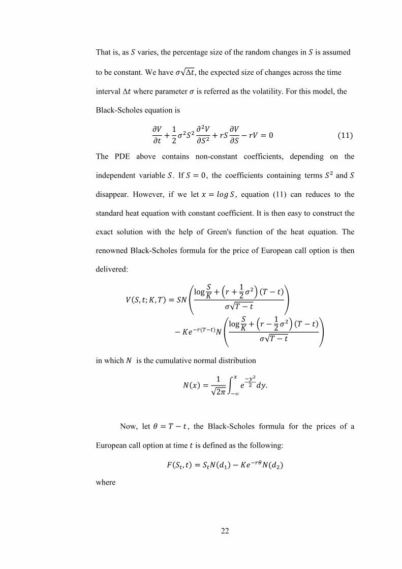
That is, as varies, the percentage size of the random changes in is assumed
to be constant. We have √∆:, the expected size of changes across the time
interval ∆: where parameter is referred as the volatility. For this model, the
Black-Scholes equation is
¢: + 12 ¢ + O ¢ − O¢ = 0 (11)
The PDE above contains non-constant coefficients, depending on the
independent variable . If = 0, the coefficients containing terms and
disappear. However, if we let . = º , equation (11) can reduces to the
standard heat equation with constant coefficient. It is then easy to construct the
exact solution with the help of Green's function of the heat equation. The
renowned Black-Scholes formula for the price of European call option is then
delivered:
¢(, :; ?, >) = ¨ »log ? + ¼O + 12 ½ (> − :) √> − : ¾− ?M¿À(¿7)¨ »log ? + ¼O − 12 ½ (> − :) √> − : ¾
in which ¨ is the cumulative normal distribution
¨(.) = 1√2' ( M¿Á 5¿∞
.
Now, let = > − : , the Black-Scholes formula for the prices of a
European call option at time : is defined as the following:
Â(7, :) = 7¨(5]) − ?M¿Àè(5)
where

23
5] = log 7? + ¼O + 12 ½ √
5 = log 7? + ¼O − 12 ½ √
= 5] − √ and ¨(∙) is the standard normal distribution function, given by
¨() = ( 1√2' M¿Á 5Á¿∞
Note that ¨() ≤ 1 if = ∞.
Using the same way, the price for European put option can also be determined.
We summarize the assumptions that are used in the model [2]:
1. The stock can be sold and bought.
• This is essential and important for constructing a hedging
portfolio. A portfolio consists of number of stocks holding and
a cash account. In order to construct a suitable hedging
portfolio, we have to keep on changing the stock holding by
selling and buying it.
2. No transaction cost is involved on buying or selling stocks.
• Here, the transaction cost refers to the charges incurred for the
transaction. It is difficult to build the transaction cost in the
model. Therefore, for simplicity, we are not considering it in
the mathematics model.

24
3. The market parameters O and are constant and known.
• The interest rate, O is differs for different customers or
investors. However, it does not have a large effect on the result.
• As mentioned before, is the volatility. The option value ¢ is a
function of and is very sensitive to .
4. No dividend.
• The underlying stock pays no dividend during the option’s life.
5. There is no arbitrage opportunity.
• No one can make a riskless profit in the market.
6. Stock price follows a Geometric Brownian motion.
• The motion of stock price cannot be predicted and move in
uncertain way. We assume that the motion follows a Geometric
Brownian motion.
3.2 Itô's Lemma Approach to Black-Scholes Equation
Geometric Brownian motion, the basic reference model for stock prices is
defined by
7 = exp(: + <7) (12)
where
25
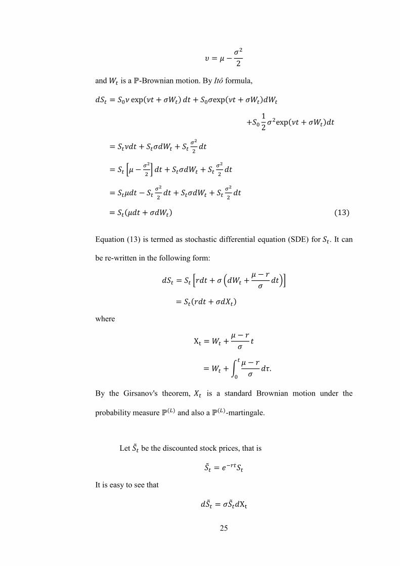
Å = 9 − 2
and <7 is a ℙ-Brownian motion. By Itô formula,
57 = exp(: + <7) 5: + exp(: + <7)5<7 + 12 exp(: + <7)5:
= 75: + 7 5<7 + 7 Æ 5:
= 7 Ç9 − Æ È 5: + 7 5<7 + 7 Æ 5:
= 795: − 7 Æ 5: + 7 5<7 + 7 Æ 5:
= 7(95: + 5<7) (13)
Equation (13) is termed as stochastic differential equation (SDE) for 7. It can
be re-written in the following form:
57 = 7 ÇO5: + ¼5<7 + 9 − O 5:½È = 7(O5: + 5b7)
where
Xg = <7 + 9 − O :
= <7 + ( 9 − O 5É7 .
By the Girsanov's theorem, b7 is a standard Brownian motion under the
probability measure ℙ(Ê) and also a ℙ(Ê)-martingale.
Let Ë7 be the discounted stock prices, that is
Ë7 = M¿À77
It is easy to see that
5Ë7 = Ë75Xg

26
Comparing with equation (13), when 9 = 0, the discounted stock prices can
now be written in the following form
Ë7 = Ëexp ,− 2 : + Xg/. and it is a ℙ(Ê)-martingale.
Let Φ = Φ(S) be the payoff function at time >. Define
7 = M¿ÀEℙ(Í)yΦ|Sg = S = Eℙ(Í)yM¿ÀΦ|Sg = S
= Eℙ(Í)yM¿ÀΦ|ℱg. By the tower property,
Eℙ(Í)y7|ℱk = Eℙ(Í) ÇyEℙ(Í)yM¿À7Φ|ℱgÎ ℱkÈ = Eℙ(Í)yM¿ÀΦ|ℱk
= p for < :. As a consequence, 7 is a ℙ(Ê)-martingale. Thus, by the Brownian
martingale representation theorem, there exists a process Ï such that we can
write 7 as an Itô integral:
7 = + ( p5bp7
= + ( p Ëp Ëp5bp7
= + ( Ðp5Ëp7
where Ðp = ÃÑÆËÑ and 5Ëp = Ëp5bp.

27
Define Ò7 = 7 − Ð7Ë7 . Then, the portfolio eÓgÒ7 + Ð7Ë7 replicate
eÓg7 , namely eÓg7 has realizable market value. As eÓg7 = Φ, the option
value at time : is then
eÓg7 = Eℙ(Í)zyM¿À(¿7)Φℱg| = Eℙ(Í)zyM¿À(¿7)ΦSg = S| (14)
Now, we introduce a new function, Â(, :). Assume that the function
Â(, :) solves the following boundary value problem
: Â(, :) + 2 Â(, :) + O Â(, :) − OÂ(, :) = 0, 0 ≤ : ≤ > Â(, :) = Φ() (15)
Define 7 = e¿ÓgÂ(, :). By Itô formula,
5 7 = 5e¿ÓgÂ(, :)
= e¿Óg ,−rÂ(, :) + Â(, :): 5: + Â(, :) 57 + 12 Â(, :) 57/
= e¿Óg ,−rÂ(, :) + Â(, :): 5: + Â(, :) (O75: + 75b7)+ 12 Â(, :) (O75: + 75b7)"
= e¿Óg ,−rÂ(, :) + Â(, :): + O7 Â(, :) + 72 Â(, :) / dt+ e¿Ógσ7 Â(, :) dXg
= e¿Ógσ7 Â(, :) dXg Then,
7 = + ( e¿ÓτσSτ
7
Â(, :) dXτ

28
is a ℙ(Ê)-martingale.
Since ¨ = e¿ÓΦ. From the martingale property,
Eℙ(Í)y¨|ℱ7 = Ng for : < >
⟹ Eℙ(Í)ye¿ÓΦ|ℱ7 = Ng ⟹ Eℙ(Í)ye¿ÓΦ|ℱ7 = e¿ÓgÂ(, :)
∴ Â(, :) = Eℙ(Í)zye¿Ó(¿g)Φℱ7| = Eℙ(Í)zye¿Ó(¿g)Φ7 = | which is actually the option value at time : that we obtained before in
expression (14).
3.3 Crank-Nicolson Finite Difference Method
Recall that the Black-Scholes model for European option:
Â: + 12 Â + O Â − OÂ = 0
Consider a function Â(, :) over a two-dimensional grid. Let © and ℎ denote
the indices for stock price, and time : respectively. At a typical point Â(, :),
write Â(, :) = ÂØ, the expression
12 Â + O Â − OÂ
is approximated by the following difference scheme
ÙØ = 2 fpp + Ofp − OÂØ
where
29
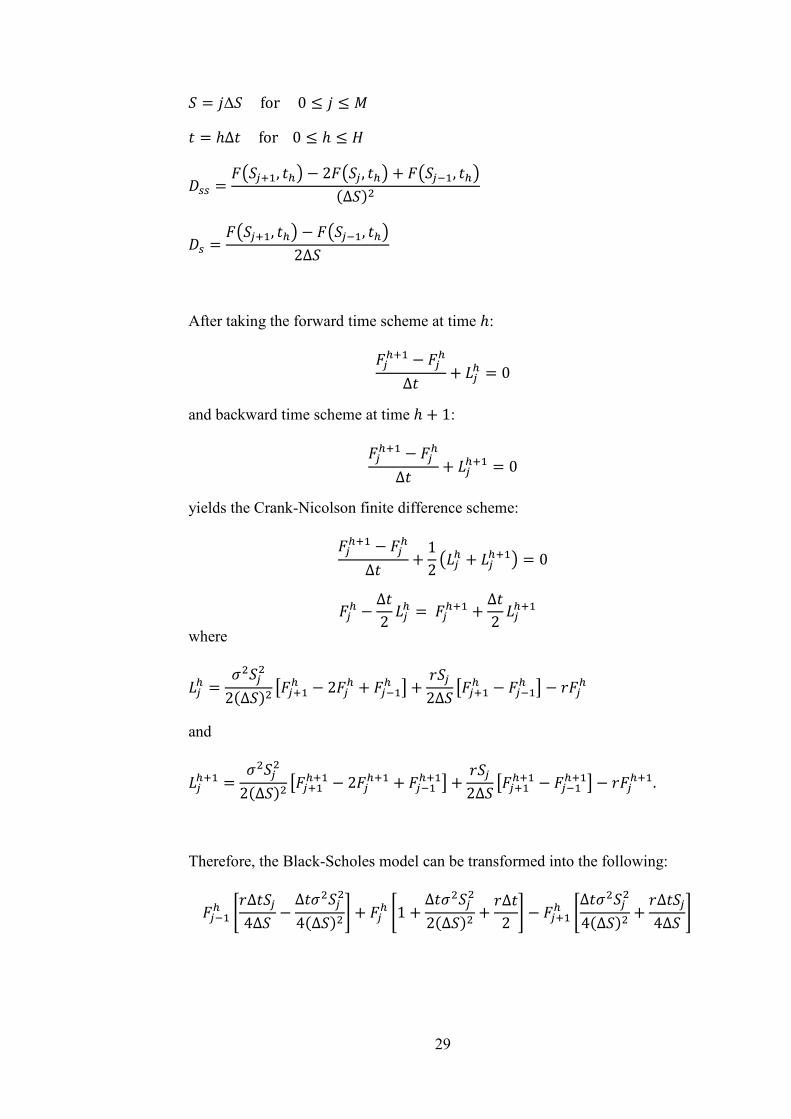
= ©∆ for 0 ≤ © ≤
: = ℎΔ: for 0 ≤ ℎ ≤ Û
fpp = Â], :Ø − 2 , :Ø + ¿], :Ø(∆)
fp = Â], :Ø − ¿], :Ø2∆
After taking the forward time scheme at time ℎ:
ÂØ] − ÂØ∆: + ÙØ = 0
and backward time scheme at time ℎ + 1:
ÂØ] − ÂØ∆: + ÙØ] = 0
yields the Crank-Nicolson finite difference scheme:
ÂØ] − ÂØ∆: + 12 ÙØ + ÙØ] = 0
ÂØ − ∆:2 ÙØ = ÂØ] + ∆:2 ÙØ] where
ÙØ = 2(∆) zÂ]Ø − 2ÂØ + ¿]Ø | + O2∆ zÂ]Ø − ¿]Ø | − OÂØ
and
ÙØ] = 2(∆) zÂ]Ø] − 2ÂØ] + ¿]Ø]| + O2∆ zÂ]Ø] − ¿]Ø]| − OÂØ].
Therefore, the Black-Scholes model can be transformed into the following:
¿]Ø 8O∆:4∆ − ∆: 4(∆) = + ÂØ 81 + ∆: 2(∆) + O∆:2 = − Â]Ø 8∆: 4(∆) + O∆:4∆ =
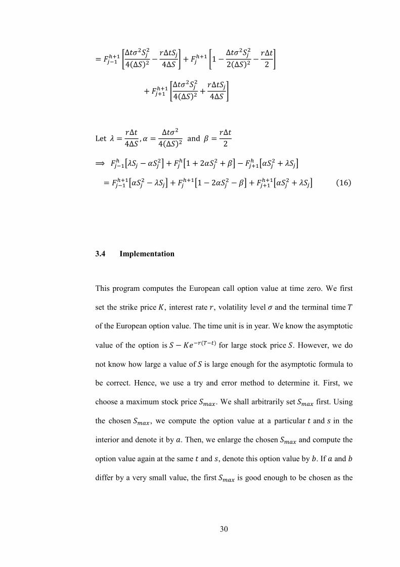
30
= ¿]Ø] 8∆: 4(∆) − O∆:4∆ = + ÂØ] 81 − ∆: 2(∆) − O∆:2 =+ Â]Ø] 8∆: 4(∆) + O∆:4∆ =
Let Ü = O∆:4∆ , Ý = ∆: 4(∆) and ß = O∆:2
⟹ ¿]Ø zÜ − Ý| + ÂØz1 + 2Ý + ß| − Â]Ø zÝ + Ü| = ¿]Ø]zÝ − Ü| + ÂØ]z1 − 2Ý − ß| + Â]Ø]zÝ + Ü| (16)
3.4 Implementation
This program computes the European call option value at time zero. We first
set the strike price ?, interest rate O, volatility level and the terminal time >
of the European option value. The time unit is in year. We know the asymptotic
value of the option is − ?M¿À(¿7) for large stock price . However, we do
not know how large a value of is large enough for the asymptotic formula to
be correct. Hence, we use a try and error method to determine it. First, we
choose a maximum stock price à4. We shall arbitrarily set à4 first. Using
the chosen à4 , we compute the option value at a particular : and in the
interior and denote it by . Then, we enlarge the chosen à4 and compute the
option value again at the same : and , denote this option value by . If and
differ by a very small value, the first à4 is good enough to be chosen as the

31
maximum stock price. à4 is usually some constant multiple of the strike
price ?.
After that, we set up the number of partition for the time, say Û and calculate
the time step 5: = á. From practical experience, we found that the accuracy of
the calculation has something to do with the ratio ââ7 . With
ââ7 = 50, both the
accuracy and computing time are reasonable. From this ratio, we then find 5.
In general, the accuracy of option price depends on the combination of number
of steps in stock price 5 and time :.
Equation (16) can be expressed in matrix form:
UÂ = ZÂ] for © = 0,1,2, … …
⇒  = U¿]ZÂ] where  = Â], , Â,,  ,, … … , Âà, ,
U =
äååæ
1 + 2Ý] + ß −(Ý + Ü) 0 ⋯ ⋯ 0 Ü] − Ý]0⋮⋮0 1 + 2Ý + ßÜ − Ý⋯⋯⋯
−(Ý + Ü´ ) 1 + 2Ý + ß⋯⋯⋯ ⋯⋯⋯⋯0
⋮⋮⋮0Üà¿] − Ýà¿]
⋮⋮0−(Ýà + Üà)1 + 2Ýà¿] + ßèééê
at time ℎ and
Z =
äååæ
1 − 2Ý] − ß Ý + Ü 0 ⋯ ⋯ 0 Ý] − Ü]0⋮⋮0 1 − 2Ý − ßÝ − Ü⋯⋯⋯
Ý + Ü´ 1 − 2Ý − ß⋯⋯⋯ ⋯⋯⋯⋯0
⋮⋮⋮0Ýà¿] − Üà¿]
⋮⋮0Ýà + Üà1 − 2Ýà¿] − ßèééê
at time ℎ + 1.
Note that the matrices U and Z are (L − 1) × (L − 1) tridiagonal matrix.

32
Since the boundary values for the option are known at terminal time, we may
perform the backward iteration to obtain the option value at time zero.
Remark: In the program code, we denote the option value (as a matrix) by H,
i.e.
HØ, = F²ì.
The Matlab function written here is named as EuropeanOption. For =20, O = 0.05, = 0.25, we may find option value by calling:
[StkPrice Call SpPrice RelErr] = EuropeanOption(20, 0.05, 0.25);
3.5 Stability Analysis
The following is a general form of Black-Scholes equation:
Â: + 12 Â + O Â − OÂ = 0
After applying Crank-Nicolson finite difference scheme, we obtained a
approximation linear system:
¿]Ø 8O∆:4∆ − ∆: 4(∆) = + ÂØ 81 + ∆: 2(∆) + O∆:2 = −Â]Ø 8∆: 4(∆) + O∆:4∆ =
= ¿]Ø] 8∆: 4(∆) − O∆:4∆ = + ÂØ] 81 − ∆: 2(∆) − O∆:2 = +Â]Ø] 8∆: 4(∆) + O∆:4∆ =.

33
Assuming the errors are propagating backward as terminal condition is given.
Let ℎ + 1 = ¨ − í and ℎ = ¨ − (í + 1).
¿]¿(î]). 8O∆:4∆ − ∆: 4(∆) = + ¿(î]). 81 + ∆: 2(∆) + O∆:2 = −Â]¿(î]). 8∆: 4(∆) + O∆:4∆ =
= ¿]¿î 8∆: 4(∆) − O∆:4∆ = + ¿î 81 − ∆: 2(∆) − O∆:2 = +Â]¿î 8∆: 4(∆) + O∆:4∆ = (17)
Solutions of equation (17) are assumed to be the following form:
¿(î]) = ï(î])Mð ñ⁄
Â]¿(î]) = ï(î])M(])ð ñ⁄
¿]¿(î]) = ï(î])M(¿])ð ñ⁄
¿î = ïî Mð ñ⁄
Â]¿î = ïî M(])ð ñ⁄
¿]¿î = ïî M(¿])ð ñ⁄ (18)
where P is a complex variable, P = √−1.
In order to find out how the error changes in time steps, substituting equations
(18) into (17), we have
ï(î])M(¿])ð ñ⁄ 8O∆:4∆ − ∆: 4(∆) = + ï(î])Mð ñ⁄ 81 + ∆: 2(∆) + O∆:2 = −ï(î])M(])ð ñ⁄ 8∆: 4(∆) + O∆:4∆ =
34
= ïî M(¿])ð ñ⁄ 8∆: 4(∆) − O∆:4∆ = + ïî Mð ñ⁄ 81 − ∆: 2(∆) − O∆:2 =
+ïî M(])ð ñ⁄ 8∆: 4(∆) + O∆:4∆ =
ï óM¿ð ñ⁄ 8O∆:4∆ − ∆: 4(∆) = + 81 + ∆: 2(∆) + O∆:2 =− Mð ñ⁄ 8∆: 4(∆) + O∆:4∆ =ô
= M¿ð ñ⁄ 8∆: 4(∆) − O∆:4∆ = + 81 − ∆: 2(∆) − O∆:2 =+ Mð ñ⁄ 8∆: 4(∆) + O∆:4∆ =
ï ó∆: 4(∆) z2 − M¿ð ñ⁄ − Mð ñ⁄ | + O∆:4∆ zM¿ð ñ⁄ − Mð ñ⁄ | + 1 + O∆:2 ô
= ∆: 4(∆) zM¿ð ñ⁄ + Mð ñ⁄ − 2| + O∆:4∆ zMð ñ⁄ − M¿ð ñ⁄ | + 1 − O∆:2
ï ó∆: 2(∆) 1 − cos(2' c⁄ ) − PO∆:2∆ sin(2' c⁄ ) + 1 + O∆:2 ô
= ∆: 2(∆) cos(2' c⁄ ) − 1 + PO∆:2∆ sin(2' c⁄ ) + 1 − O∆:2
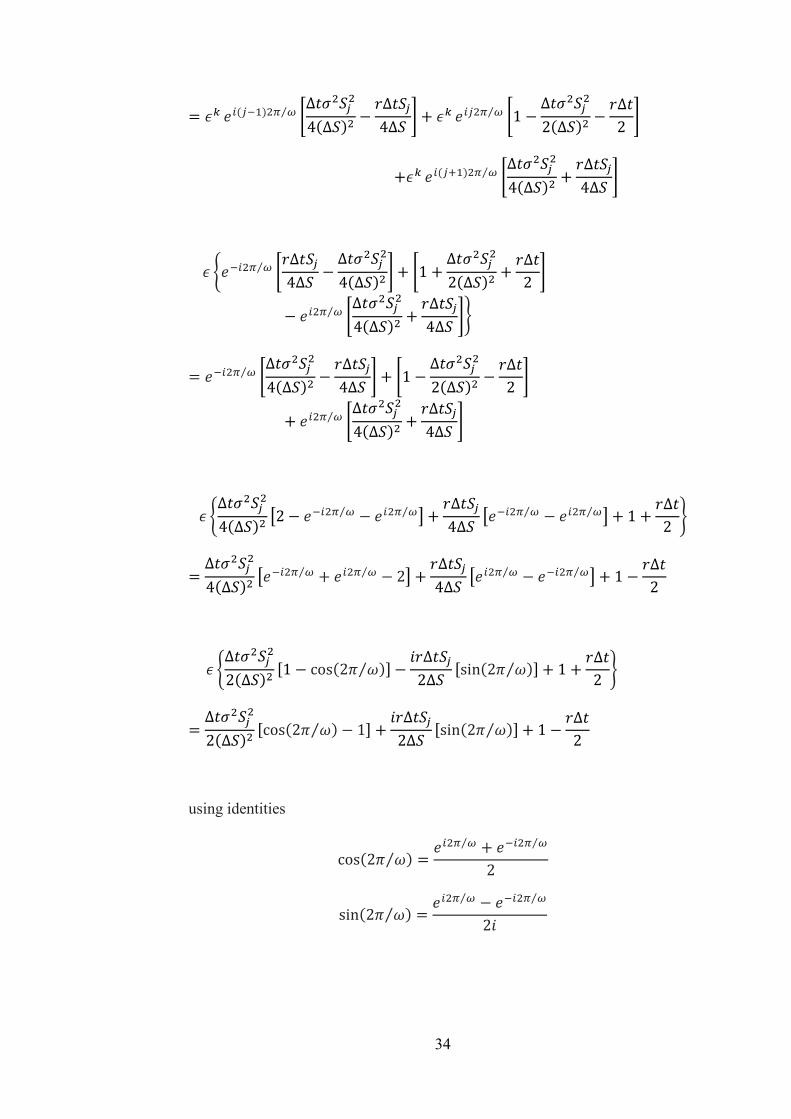
using identities
cos(2' c⁄ ) = Mð ñ⁄ + M¿ð ñ⁄2
sin(2' c⁄ ) = Mð ñ⁄ − M¿ð ñ⁄2P

35
By the von Neumann stability analysis (also known as Fourier stability
analysis), if |ï| ≤ 1, the difference equation is stable and vice-versa.
|ï| = ÷8∆: 2(∆) cos(2' c⁄ ) − 1 + 1 − O∆:2 = + 8O∆:2∆ sin(2' c⁄ )=
÷8∆: 2(∆) 1 − cos(2' c⁄ ) + 1 + O∆:2 = + 8− O∆:2∆ sin(2' c⁄ )=
= ÷81 − ,∆: 2(∆) 1 − cos(2' c⁄ ) + O∆:2 /= + 8O∆:2∆ sin(2' c⁄ )=
÷81 + ,∆: 2(∆) 1 − cos(2' c⁄ ) + O∆:2 /= + 8− O∆:2∆ sin(2' c⁄ )=
Since
∆: 2(∆) 1 − cos(2' c⁄ ) + O∆:2 ≥ 0, we have
|ï| ≤ 1.
3.6 Simulation and Analysis
Table below shows the results of different set of parameters with different
initial stock price S:
36
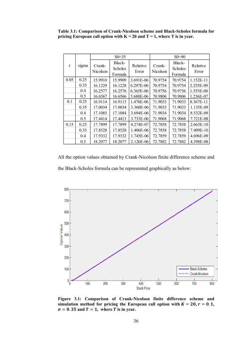
Table 3.1: Comparison of Crank-Nicolson scheme and Black-Scholes formula for
pricing European call option with K = 20 and T = 1, where T is in year.
Crank-
Nicolson
Black-
Scholes
Formula
Relative
Error
Crank-
Nicolson
Black-
Scholes
Formula
Relative
Error
0.05 0.25 15.9910 15.9909 3.691E-06 70.9754 70.9754 1.152E-11
0.35 16.1229 16.1228 6.297E-06 70.9754 70.9754 2.255E-09
0.4 16.2577 16.2576 6.365E-06 70.9756 70.9756 1.553E-08
0.5 16.6567 16.6566 5.688E-06 70.9806 70.9806 1.236E-07
0.1 0.25 16.9114 16.9113 1.478E-06 71.9033 71.9033 8.367E-11
0.35 17.0034 17.0034 3.360E-06 71.9033 71.9033 1.135E-09
0.4 17.1085 17.1084 3.694E-06 71.9034 71.9034 8.532E-09
0.5 17.4414 17.4413 3.733E-06 71.9068 71.9068 7.721E-08
0.15 0.25 17.7899 17.7899 4.274E-07 72.7858 72.7858 2.663E-10
0.35 17.8528 17.8528 1.406E-06 72.7858 72.7858 7.409E-10
0.4 17.9332 17.9332 1.745E-06 72.7859 72.7859 4.696E-09
0.5 18.2077 18.2077 2.126E-06 72.7882 72.7882 4.398E-08
r sigma
S0=35 S0=90
All the option values obtained by Crank-Nicolson finite difference scheme and
the Black-Scholes formula can be represented graphically as below:
Figure 3.1: Comparison of Crank-Nicolson finite difference scheme and
simulation method for pricing the European call option with ø = ùú, û = ú. , ü = ú. ýþ and I = , where I is in year.
37
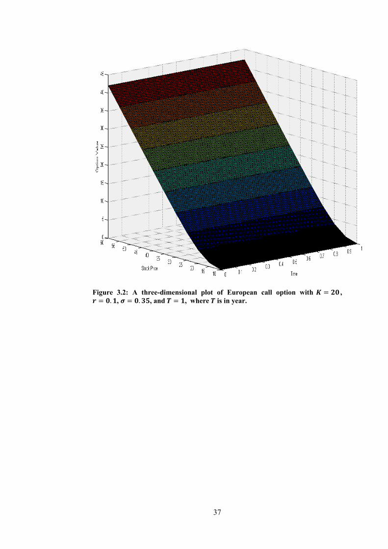
Figure 3.2: A three-dimensional plot of European call option with ø = ùú , û = ú. , ü = ú. ýþ, and I = , where I is in year.

38
Figure 3.3: A three-dimensional plot of European call option with ø = þú , û = ú. , ü = ú. ýþ, and I = , where I is in year.
3.7 Conclusion
Obviously, the option values obtained by proposed method are quite agreeable
with the Matlab build-in function method. It is considered as consistent under
different initial stock price and also volatility level.
39
CHAPTER 4
ASIAN OPTION – A TWO-DIMENSIONAL PDE
4.1 Introduction
Recall that Asian option is an option based on the average price of the
underlying stock over the lifetime of the option. The term “Asian” is a reserved
word and has no particular significance. Bankers David Spaughton told the
story of how both he and Mark Standish were both working for Bankers Trust
in 1987. They were in Tokyo, Japan on business when they found this method
of pricing option. Hence, they called the option as Asian option.
Asian option is not traded as a standardized contract in any organized
exchange. However, it is popular in the over-the-counter (OTC) market. There
are several reasons for introducing Asian option. For instance, a corporation
expecting to make payment in foreign currency can reduce its average foreign
currency exposure by using Asian option. Besides, introducing Asian option
can also avoid manipulation of the stock near expiration time. Stock price at
time is subject to manipulation. However, it is not easy to manipulate if we
average the stock price.
40
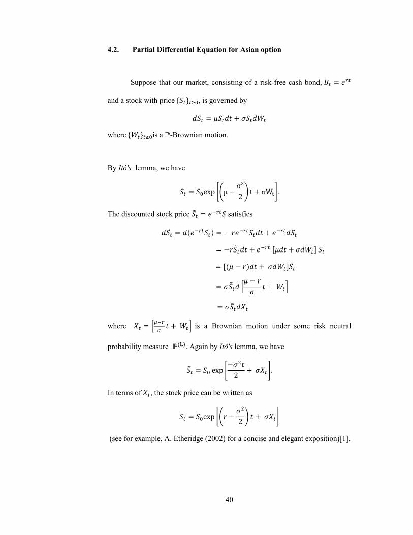
4.2. Partial Differential Equation for Asian option
Suppose that our market, consisting of a risk-free cash bond,
and a stock with price , is governed by
where is a -Brownian motion.
By Itô's lemma, we have
exp µ σ2 t σW. The discounted stock price ! " satisfies
! #"$ &" "
&! " ' ( '# &$ (!
! ) & * !+
where + ),"- * is a Brownian motion under some risk neutral
probability measure #L$. Again by Itô's lemma, we have
! exp 2 +. In terms of +, the stock price can be written as
exp & 2 +
(see for example, A. Etheridge (2002) for a concise and elegant exposition)[1].

41
Let ΦT Φ#01 , 1$ max #56T K, 0$ be the payoff function at time
where 1 refers to the stock price at time and 56T refers to the average stock
price at time and where 0 9 :; .
From our general theory [1], option value at time is given by:
V#Z, S$ e"?#T"$E#L$'Φ#01 , 1$|B( e"?#T"$E#L$'Φ#01 , 1$|S S, Z Z(
where #C$ is the risk neutral probability measure under which the discounted
stock price ! " is a #C$-martingale.
Now, we introduce a new function, D#0, , $ which solves the terminal
value problem
EDE & EDE 12 EDE E0E EDE0 &D 0 #19$
D#0, , $ Φ#0, $.
Define H "D#0, , $ . Recall that #& +$ . By the Itô's
formula,
H #"D#0, , $$
" &D EDE EDE 12 EDE EDE0 0 " &D EDE EDE #& +$
12 EDE #& +$ EDE0 0I

42
" &D EDE & EDE 12 EDE EDE0 0E
" EDE +
" EDE +. It follows that
N N K "?τσSτ
EDE +
is a #C$-martingale. Since H1 "1ΦT, by martingale property,
L#M$'H1|B( H
L#M$'"1Φ1|B( H
L#M$'"1Φ1|B( "D#, 0, $
N D#0, , $ L#M$O"#1"$Φ1PBQ L#M$O"#1"$Φ1P , 0 0Q is the option value at time .
Since the diffusion term RSTR5S is missing, equation (19) is a degenerate
diffusion equation. As
0 K :; ,
E0E , equation (19) now assumes the form,
EDE & EDE 12 EDE EDE0 &D 0
D#0, , $ Φ#0, $ #20$

43
4.3 Method of Solution
There are two problems concerning equation (20).
(a). To determine if equation (20) is a well posed problem.
(b). To propose an efficient difference scheme for solving it.
Problem (a) will not be treated here because equation (20) is a degenerate two-
dimensional diffusion equation which is known to be a well posed problem
under special boundary conditions. The far field boundary conditions are
provided by Kangro [21]. The other suitable boundary conditions are derived in
the following section.
4.4. Boundary Values
First, we consider the left boundary condition. We found that 0 implies : 0 for ; U and 01 9 :;1 9 :; 9 :;1 0 .
Hence for the Asian call option with payoff DV#01 , 1 , $ #561 W$X, when
0, we obtain
DV#0, 0, $ E#M$ Y"#1"$#0 W$X| 0, 0 0I
"#1"$#0 W$X as the left boundary condition.
Next we derive the call option price DV#0, , $ at time when it is in
money, that is, when 5Z1 U W.
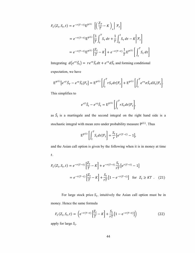
44
DV#0, , $ "#1"$E#M$ Y[\ 01 W ]X^ BI "#1"$E#M$ [1 K :1
; 1 K : ; W_ B
"#1"$E#M$ Y0 WI "#1"$ 1 E#M$ K :1 ;
Integrating `!a &! ! and forming conditional
expectation, we have
E#M$O1!1 !|BQ E#M$ K &:;|B [1 E#M$ K :!:+|B [1
. This simplifies to
1! ! E#M$ K &:;|B [1 ,
as ! is a martingale and the second integral on the right hand side is a
stochastic integral with mean zero under probability measure #C$. Thus
E#M$ K :;|B [1 & O#1"$ 1Q,
and the Asian call option is given by the following when it is in money at time
.
DV#0, , $ "#1"$ Y0 WI "#1"$ & O#1"$ 1Q "#1"$ Y0 WI & O1 "#1"$Q for 0 e W . #21$
For large stock price , intuitively the Asian call option must be in
money. Hence the same formula
DV#0 , , $ \e"#1"$ Y0 WI & O1 e"#1"$Q] #22$
apply for large .
45
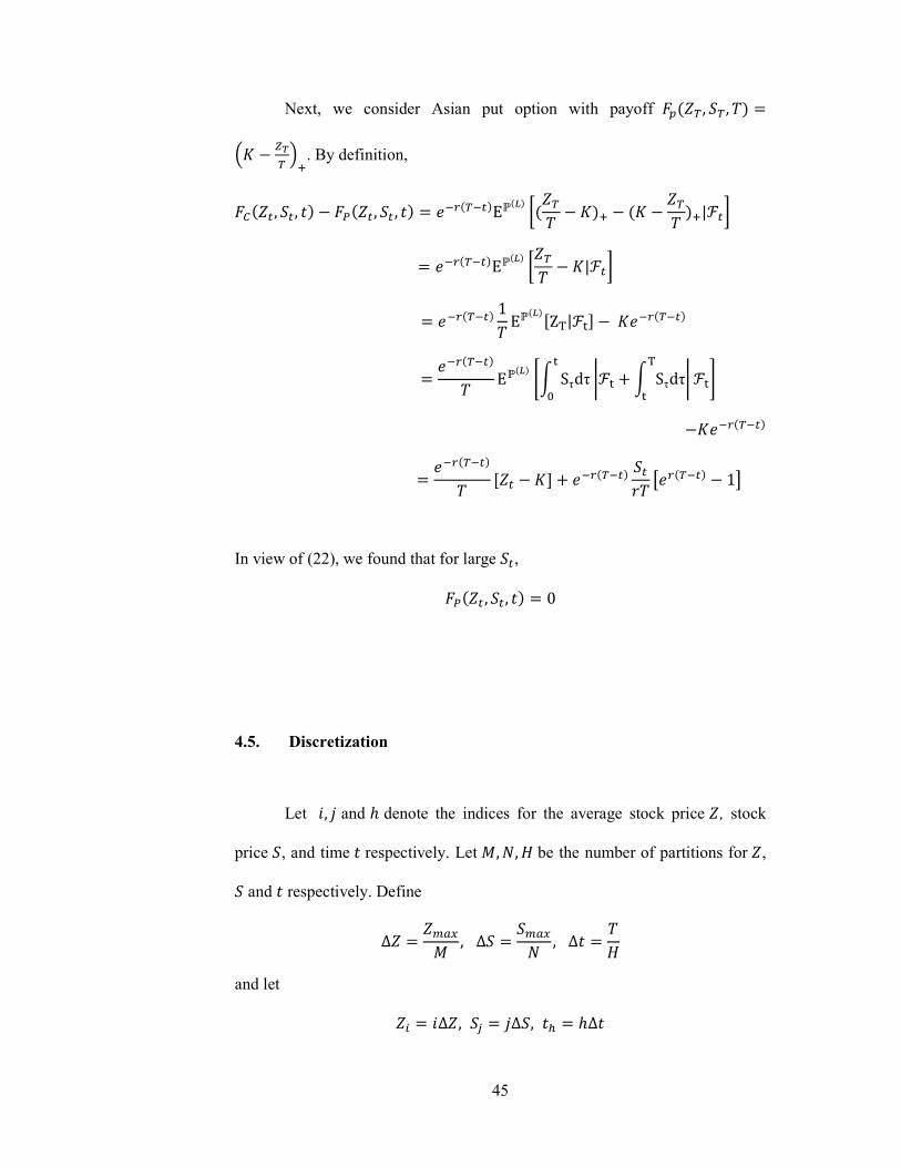
Next, we consider Asian put option with payoff Df#01 , 1 , $ gW 561 hX. By definition,
DV#0, , $ Di#0, , $ "#1"$E#M$ Y#01 W$X #W 01 $X|BI
"#1"$E#M$ Y01 W|BI
"#1"$ 1 E#M$'ZT|B [( W"#1"$ "#1"$ E#M$ K Sτdτ _B [K Sτdτ
T _ B [
W"#1"$ "#1"$ '0 W( "#1"$ & O#1"$ 1Q
In view of (22), we found that for large ,
Di#0 , , $ 0
4.5. Discretization
Let k, l and m denote the indices for the average stock price 0, stock
price , and time respectively. Let n, H, o be the number of partitions for 0,
and respectively. Define
∆0 0qrsn , ∆ qrsH , ∆ o
and let
0t k∆0, u l∆, v m∆

46
for
0 w k w n, 0 w l w H, 0 w m w o.
Figure 4.1 : A three-dimensional grid
The nodes #0t , u , v$ form a uniform grid in '0, 0qrs( x '0, qrs( x '0, (. At
a node #k, l, m$ y #0t, u , v$ the expression
2 EDE & EDE EDE0 &D
is approximated by the difference scheme
zt,uv u2 || &u| u5 &Dt,uv
where
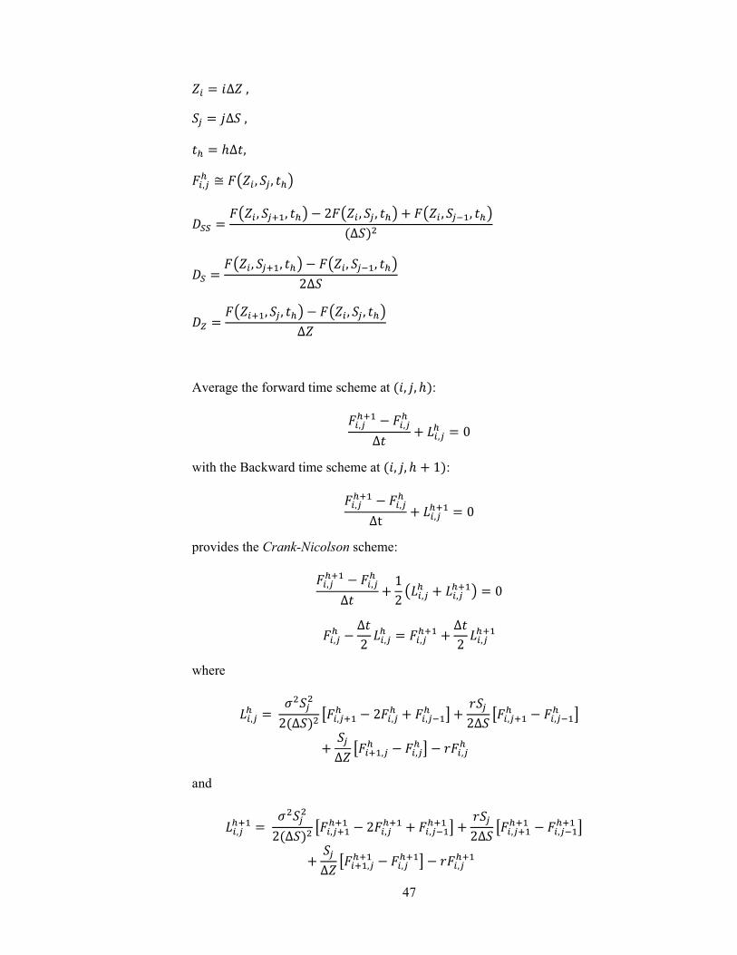
47
0t k∆0 , u l∆ , v m∆, Dt,uv D`0t , u, va || D`0t , uX~, va 2D`0t , u , va D`0t , u"~, va#∆$
| D`0t, uX~, va D`0t, u"~, va2∆
5 D`0tX~, u, va D`0t , u , va∆0
Average the forward time scheme at #k, l, m$:
Dt,uvX~ Dt,uv∆ zt,uv 0 with the Backward time scheme at #k, l, m 1$:
Dt,uvX~ Dt,uv∆t zt,uvX~ 0
provides the Crank-Nicolson scheme:
Dt,uvX~ Dt,uv∆ 12 `zt,uv zt,uvX~a 0
Dt,uv ∆2 zt,uv Dt,uvX~ ∆2 zt,uvX~
where
zt,uv u2#∆$ ODt,uX~v 2Dt,uv Dt,u"~v Q &u2∆ ODt,uX~v Dt,u"~v Q u∆0 ODtX~,uv Dt,uv Q &Dt,uv
and
zt,uvX~ u2#∆$ ODt,uX~vX~ 2Dt,uvX~ Dt,u"~vX~ Q &u2∆ ODt,uX~vX~ Dt,u"~vX~ Q u∆0 ODtX~,uvX~ Dt,uvX~Q &Dt,uvX~

48
Therefore,
&∆u4∆ ∆u4#∆$ Dt,u"~v 1 ∆u2#∆$ ∆u2∆0 &∆2 Dt,uv &∆u4∆ ∆u4#∆$ Dt,uX~ v ∆u2∆0 DtX~,uv
∆u4#∆$ &∆u4∆ Dt,u"~vX~ 1 ∆u2#∆$ ∆u2∆0 &∆2 Dt,uvX~
∆u4#∆$ &∆u4∆ Dt,uX~ vX~ ∆u2∆0 DtX~,uvX~
Let -S∆#∆|$S , ∆∆|, and ∆∆5. The above may be abbreviated to
`u uaDt,u"~v `1 2u u 2∆aDt,uv
`u uaDt,uX~v uDtX~,uv `u uaDt,u"~vX~ `1 2u u 2∆aDt,uvX~
`u uaDt,uX~vX~ uDtX~,u vX~ #23$
The figure below is a visualization of the equation above :
Figure 4.2: Relationship between values of at several points
49
Note that Dt,uv D#k, l, m$ is the option price at time m∆, average stock price
k∆ and stock price l∆. As depicted in the Figure 4.2, equation (23) represents
a relationship between values of Dat the 8 points#k, l, m$, #k, l 1, m$, #k, l 1, m$, #k 1, l, m$, #k, l, m 1$, #k, l 1, m 1$, #k, l 1, m 1$, #k 1, l, m 1$. At the time of computation, if values of D at 5 points #k 1, l, m$, #k, l, m 1$, #k, l 1, m 1$, #k, l 1, m 1$, #k 1, l, m 1$ are known, then values of
D at #k, l, m$, #k, l 1, m$, #k, l 1, m$, satisfy linear equation (23). This is the
case if starting at and 0 0qrs, iteration is performed backward in time
and in 0 . For fixed m and k , corresponding to each of the interior points
#k, l, m$ where l 1,2, . . 1, there is one and only one linear equation (23)
and therefore there are as many equations as unknowns D#k, l, m$ for l 1,2, . . 1and D#k, l, m$ may be determined.
4.6. Implementation
The way to calculate the value of Asian option at time zero is similar to the
way of finding the value of European option. First of all, we set all the given
parameters: terminal time , maximum stock price qrs , strike price W ,
interest rate & and volatility level . We then determine the maximum average
stock price as 0qrs W because this would make the payoff function equals
to zero. Finally, we determine , 0 and based on their number of
partitions. Note that the time unit is in year.

50
Let and be the matrices for time m and m 1 respectively defined
as follows:
At time m,
1 2~ ~ 2Δ # $ 0 0 ~ ~001 2 2Δ
# $1 2 2Δ0
0"~ "~
0# $1 2 2Δ
At time m 1,
1 2~ ~ 2Δ 0 0 ~ ~001 2 2Δ
1 2 2Δ0
0"~ "~
0 1 2 2Δ
Note that the matrices and are tridiagonal matrices with size # 1$ x# 1$ where .
Write system (23) in matrix form: Dv DvX~ where Dv #Dt,~v ,Dt,v , … . . Dt,"~v $1 and is the column vector arising from boundary values.
Solving, yield Dv "~DvX~ "~.
When 0 U W , option price can be calculated according to equation (21).
Hence option price is only computed using finite difference scheme when
0 w W. Below are the boundary conditions that we found previously:
1. DV#01 , 1 , $ g561 WhX
2. When stock price is zero,
DV#0, 0, $ e"?#T"$ g51 WhX

51
3. DV#0 , , $ e"?#T"$ g5Z1 Wh S?T O1 e"?#T"$Q for 0 e W
4. DV#0 , 1 , $ e"?#T"$ g5Z1 Wh S?T O1 e"?#T"$Q if stock price is
large.
To compute the value of Asian option, just call our function AsianOption
(Appendix B) with proper parameters. For instance,
[StkPrice CallPrice SpPrice RelErr] = AsianOption(20, 0.1, 0.5)
4.7. Stability Analysis
Recall that the following is the approximate difference equation after applying
Crank-Nicolson scheme:
Dt,u"~v &∆u4∆ ∆u4#∆$ Dt,uv 1 ∆u2#∆$ ∆u2∆0 &∆2
Dt,uX~ v &∆u4∆ ∆u4#∆$ DtX~,uv ∆u2∆0 Dt,u"~vX~ ∆u4#∆$ &∆u4∆ Dt,uvX~ 1 ∆u2#∆$ ∆u2∆0 &∆2
Dt,uX~ vX~ ∆u4#∆$ &∆u4∆ DtX~,uvX~ ∆u2∆0 which is derived from the general form of Black-Scholes equation:
EDE & EDE 12 EDE EDE0 &D 0

52
Let m 1 H and m H # 1$, we have
Dt,u"~"#X~$ &∆u4∆ ∆u4#∆$ Dt,u"#X~$ 1 ∆u2#∆$ ∆u2∆0 &∆2
Dt,uX~ "#X~$ &∆u4∆ ∆u4#∆$ DtX~,u"#X~$ ∆u2∆0 Dt,u"~" ∆u4#∆$ &∆u4∆ Dt,u" 1 ∆u2#∆$ ∆u2∆0 &∆2
Dt,uX~ " ∆u4#∆$ &∆u4∆ DtX~,u" ∆u2∆0 #24$
Solutions of equation (24) are assumed to be the following:
Dt,u"#X~$ #X~$#tXu$√"~ ¡⁄ Dt,uX~"#X~$ #X~$#tXuX~$√"~ ¡⁄
Dt,u"~"#X~$ #X~$#tXu"~$√"~ ¡ ⁄
DtX~,u"#X~$ #X~$ #tXuX~$√"~ ¡⁄
Dt,u" #tXu$√"~ ¡⁄ Dt,uX~" #tXuX~$√"~ ¡⁄ Dt,u"~" #tXu"~$√"~ ¡⁄
DtX~,u" #tXuX~$√"~ ¡⁄ (25)
Note that the k here refers to an index. Now, substituting equations (25) into
(24), we have
#X~$#tXu"~$√"~ ¡⁄ &∆u4∆ ∆u4#∆$ #X~$#tXu$√"~ ¡⁄ 1 ∆u2#∆$ ∆u2∆0 &∆2 #X~$#tXuX~$√"~ ¡⁄ &∆u4∆ ∆u4#∆$ #X~$ #tXuX~$√"~ ¡⁄ Y∆u2∆0I

53
#tXu"~$√"~ ¡⁄ ∆u4#∆$ &∆u4∆ #tXu$√"~ ¡⁄ 1 ∆u2#∆$ ∆u2∆0 &∆2
#tXuX~$√"~ ¡⁄ ∆u4#∆$ &∆u4∆
#tXuX~$√"~ ¡⁄ Y∆u2∆0I
£"√"~ ¡⁄ &∆u4∆ ∆u4#∆$ 1 ∆u2#∆$ ∆u2∆0 &∆2 √"~ ¡⁄ &∆u4∆ ∆u4#∆$ ∆u2∆0¤
"√"~ ¡⁄ ∆u4#∆$ &∆u4∆ 1 ∆u2#∆$ ∆u2∆0 &∆2
√"~ ¡⁄ ∆u4#∆$ &∆u4∆ ∆u2∆0
£∆u4#∆$ O2 `"√"~ ¡⁄ √"~ ¡⁄ aQ &∆u4∆ O"√"~ ¡⁄ √"~ ¡⁄ Q ∆u2∆0 O√"~ ¡⁄ Q 1 ∆u2∆0 &∆2 ¤
∆u4#∆$ O"√"~ ¡⁄ √"~ ¡⁄ 2Q &∆u4∆ O√"~ ¡⁄ "√"~ ¡⁄ Q ∆u2∆0 O√"~ ¡⁄ Q 1 ∆u2∆0 &∆2
£∆u4#∆$ '2 2 cos#2§ ¨⁄ $( &∆u4∆ O2√1 sin#2§ ¨⁄ $Q ∆u2∆0 Ocos#2§ ¨⁄ $ √1 sin#2§ ¨⁄ $Q 1 ∆u2∆0 &∆2 ¤
54
∆u4#∆$ '2 cos#2§ ¨⁄ $ 2( &∆u4∆ O2√1 sin#2§ ¨⁄ $Q ∆u2∆0 Ocos#2§ ¨⁄ $ √1 sin#2§ ¨⁄ $Q 1 ∆u2∆0 &∆2
£∆u2#∆$ '1 cos#2§ ¨⁄ $( ∆u2∆0 '1 cos#2§ ¨⁄ $( 1 &∆2 &∆u2∆ O√1 sin#2§ ¨⁄ $Q ∆u2∆0 O√1 sin#2§ ¨⁄ $Q¤
∆u2#∆$ 'cos#2§ ¨⁄ $ 1( ∆u2∆0 'cos#2§ ¨⁄ $ 1( 1 &∆2 &∆u2∆ O√1 sin#2§ ¨⁄ $Q ∆u2∆0 O√1 sin#2§ ¨⁄ $Q
using identities
√"~ ¡⁄ cos#2§ ¨⁄ $ √1 sin#2§ ¨⁄ $
cos#2§ ¨⁄ $ √"~ ¡⁄ "√"~ ¡⁄2
sin#2§ ¨⁄ $ √"~ ¡⁄ "√"~ ¡⁄2√1
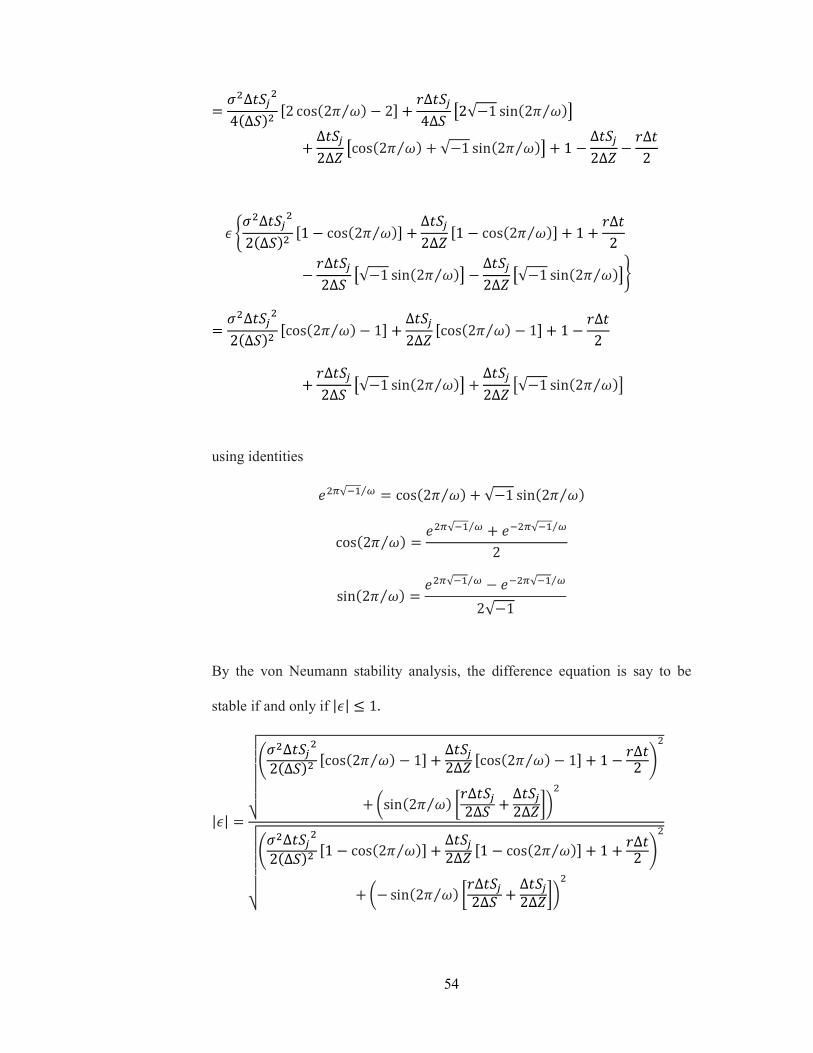
By the von Neumann stability analysis, the difference equation is say to be
stable if and only if || w 1.
|| «¬¬¬¬¬¬¬¬∆u2#∆$ 'cos#2§ ¨⁄ $ 1( ∆u2∆0 'cos#2§ ¨⁄ $ 1( 1 &∆2
\sin#2§ ¨⁄ $ Y&∆u2∆ ∆u2∆0I]
«¬¬¬¬¬¬¬¬∆u2#∆$ '1 cos#2§ ¨⁄ $( ∆u2∆0 '1 cos#2§ ¨⁄ $( 1 &∆2
\ sin#2§ ¨⁄ $ Y&∆u2∆ ∆u2∆0I]

55
«¬¬¬¬¬¬¬¬1 ∆u2#∆$ '1 cos#2§ ¨⁄ $( ∆u2∆0 '1 cos#2§ ¨⁄ $( &∆2
\sin#2§ ¨⁄ $ Y&∆u2∆ ∆u2∆0I]
«¬¬¬¬¬¬¬¬1 ∆u2#∆$ '1 cos#2§ ¨⁄ $( ∆u2∆0 '1 cos#2§ ¨⁄ $( &∆2
\ sin#2§ ¨⁄ $ Y&∆u2∆ ∆u2∆0I]
®1 ¯'1 cos#2§ ¨⁄ $( ∆u2#∆$ ∆u2∆0 &∆2 ° \sin#2§ ¨⁄ $ Y&∆u2∆ ∆u2∆0I]
±1 ¯'1 cos#2§ ¨⁄ $( ∆u2#∆$ ∆u2∆0 &∆2 ° \ sin#2§ ¨⁄ $ Y&∆u2∆ ∆u2∆0I]
Since
'1 cos#2§ ¨⁄ $( ∆u2#∆$ ∆u2∆0 &∆2 e 0, we have
|| w 1.
4.8. Simulation and Analysis
Table below compares results obtained by Crank-Nicolson scheme for
two-dimensional PDE and by CRR Binomial Tree method (Matlab Build-in
function) for pricing the Asian option for a variety of parameters combinations.
56
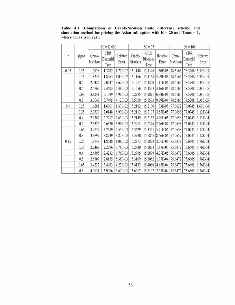
Table 4.1: Comparison of Crank-Nicolson finite difference scheme and
simulation method for pricing the Asian call option with K = 20 and Tmax = 1,
where Tmax is in year.
Crank-
Nicolson
CRR
Binomial
Tree
Relative
Error
Crank-
Nicolson
CRR
Binomial
Tree
Relative
Error
Crank-
Nicolson
CRR
Binomial
Tree
Relative
Error
0.05 0.25 1.3938 1.3702 1.72E-02 15.1148 15.1146 1.50E-05 78.5166 78.5208 5.39E-05
0.35 1.8253 1.8065 1.04E-02 15.1166 15.1158 4.99E-05 78.5166 78.5208 5.39E-05
0.4 2.0422 2.0247 8.62E-03 15.1217 15.1200 1.11E-04 78.5166 78.5208 5.39E-05
0.5 2.4762 2.4603 6.48E-03 15.1556 15.1508 3.16E-04 78.5166 78.5208 5.39E-05
0.65 3.1241 3.1089 4.90E-03 15.2995 15.2891 6.84E-04 78.5166 78.5208 5.39E-05
0.8 3.7649 3.7495 4.12E-03 15.5659 15.5503 9.99E-04 78.5166 78.5208 5.36E-05
0.1 0.25 1.6281 1.6061 1.37E-02 15.2102 15.2100 1.33E-05 77.0622 77.0745 1.60E-04
0.35 2.0329 2.0148 8.99E-03 15.2112 15.2107 3.57E-05 77.0658 77.0745 1.12E-04
0.4 2.2387 2.2217 7.63E-03 15.2149 15.2137 8.00E-05 77.0658 77.0745 1.12E-04
0.5 2.6526 2.6370 5.90E-03 15.2413 15.2376 2.46E-04 77.0658 77.0745 1.12E-04
0.65 3.2737 3.2589 4.55E-03 15.3629 15.3541 5.71E-04 77.0658 77.0745 1.12E-04
0.8 3.8899 3.8749 3.87E-03 15.5990 15.5855 8.66E-04 77.0659 77.0745 1.12E-04
0.15 0.25 1.8748 1.8548 1.08E-02 15.2873 15.2874 2.36E-06 75.6472 75.6605 1.76E-04
0.35 2.2469 2.2296 7.76E-03 15.2880 15.2878 1.18E-05 75.6472 75.6605 1.76E-04
0.4 2.4395 2.4232 6.76E-03 15.2905 15.2899 4.37E-05 75.6472 75.6605 1.76E-04
0.5 2.8307 2.8155 5.38E-03 15.3109 15.3082 1.77E-04 75.6472 75.6605 1.76E-04
0.65 3.4227 3.4083 4.23E-03 15.4132 15.4060 4.63E-04 75.6472 75.6605 1.76E-04
0.8 4.0131 3.9986 3.62E-03 15.6217 15.6102 7.37E-04 75.6472 75.6605 1.76E-04
r sigma
S0 = K =20 S0 = 35 S0 = 100

57
The following figure shows the option value obtained by two different methods
under different stock price:
Figure 4.3: Comparison of Crank-Nicolson finite difference scheme and
simulation method for pricing the Asian call option under different stock price
with ² ³´, µ ´. ¶, · ´. ³¸, and ¹ ¶, where ¹ is in year.
58
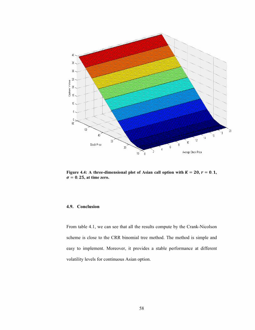
Figure 4.4: A three-dimensional plot of Asian call option with ² ³´, µ ´. ¶, · ´. ³¸, at time zero.
4.9. Conclusion
From table 4.1, we can see that all the results compute by the Crank-Nicolson
scheme is close to the CRR binomial tree method. The method is simple and
easy to implement. Moreover, it provides a stable performance at different
volatility levels for continuous Asian option.

59
CHAPTER 5
ASIAN OPTION - A ONE-DIMENSIONAL PDE
5.1. Introduction
As discussed in previous chapter, prices of Asian option can be
obtained by solving a two-dimensional PDE using a Crank-Nicolson finite
difference scheme. Recently, through a change of numéraire argument, Jan
Večeř obtained a one -dimensional heat equation whose solution leads to
Asian option pricing [13]. This one-dimensional heat equation will be derived
here and then solved by a Crank-Nicolson finite difference scheme.
5.2. Change of Numéraire Argument
Assume that
,
where , 0 , is a Brownian motion under the risk-neutral measure
. Recall that an Asian call option is an option with payoff
max 1
max !" #.

60
Let & be a deterministic function of for 0 . To price this call, we
create a portfolio process ', consisting of & number of shares of the
risky asset and bank borrowing or depositing for 0 .
We select & properly so that
' 1 .
First, note that
()*& +()*&, ()*&.
At time , we buy & units of stock and deposit balance ' &
into the bank. Thus
' & ' &, or
' ' & . Now
-()*'. ()*' '
()*&
+()*&, ()*&.
Integrating yields
()*'
()'0 -()*/&00. ()*/0&0
()'0 ()&00 ()*& ()*/0&0
which reduce to
()*& 1 00 ,

61
if we select
'0 1 1 (*)0 (*)
& 1 +1 (*)*, for 0 . Therefore,
' 1 +1 (*)*, (*)* (*)* 1 00 ,
for
0 .
In particular,
' 1 00 , 0 .
In terms of ' , the payoff is
'4 max5' , 06, and at time , the price of Asian call option is
789(*)* :;< 789(*)*'4 :;<.
To evaluate this conditional expectation, let
= ' (*)'(*)
be the portfolio value in terms of the number of the stocks. This is a change of
numéraire. We have changed the unit of account from dollars to assets.
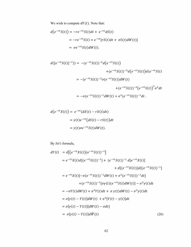
62
We wish to compute =. Note that:
+(*), (*) (*) (*) (*)> ? (*).
>(*)?*@ (*)*A+(*),
(*)*B+(*),(*)
(*)*A(*)
(*)*B+(*),AA
(*)*@ A(*)*@ .
+(*)', (*)' '
&(*)+ ,
&(*).
By Itô's formula,
= 9+(*)',(*)*@< (*)'>(*)*@? (*)*@ >(*)'?
>(*)'?>(*)*@? (*)'>(*)*@ A(*)*@?
(*)*@>&(*)? A& = A= & A&
>& =? A>= &? >& =?> ? >& =?C (26)
63
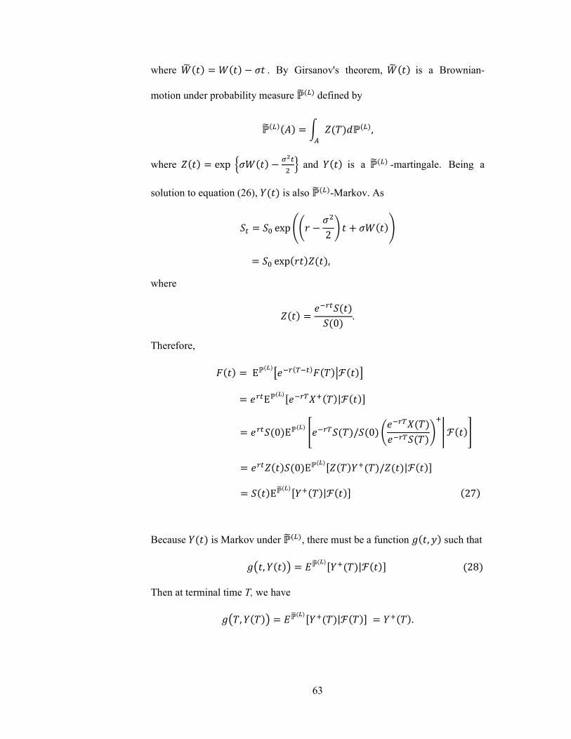
where C . By Girsanov's theorem, C is a Brownian-
motion under probability measure C defined by
CD " E , where " exp H IJ
A K and = is a C -martingale. Being a
solution to equation (26), = is also C-Markov. As
exp L A2 N
exp", where
" (*)0 . Therefore,
E89(*)* :;< ()E8>(*)'4 |;?
()0E8 QR(*) /0 (*)' (*) 4T ;U ()"0E8>R" =4 /"|;?
EC8>R=4 |;? 27
Because = is Markov under C, there must be a function W, X such that
W+, =, 7C8>R=4 |;? 28
Then at terminal time T, we have
W+ , = , 7C8>R=4 |; ? =4 .

64
5.3. Boundary Values
Recall that = Z[ represents the portfolio value in term of the number of
stocks held. As the value for ' is positive or negative while is always
positive, = is either positive or negative. When = is very negative, the
probability that = is negative or =4 0 is near one. This leads to the
condition
lim^_*∞W, X 0 , 0 .
On the other hand, when = is positive and large, the probability that
= ` 0 is near one. Therefore, for large =
W+, =, 7C8>R=4 |;? 7C8>R= |;?
=. This gives raise to the boundary condition
lim^_∞>W, X X? 0 , 0 .
At the terminal time , we also have W , X X4 as the top boundary
condition.
Note that the domain for X is unbounded. In numerical calculation, we have to
compute in a finite domain. So, we need to truncate the unbounded domain
into a bounded domain by setting the maximum value for X.

65
5.4. Partial Differential Equation for Asian option
In this section, we will derive the one-dimensional heat equation for W, X by
obtaining its differential:
W+, =, W+, =, W^+, =,= 12 W^^+, =,==
W+, =, W^+, =,9+& =,C < 12 W^^+, =, aA& =A+C ,Ab
cW+, =, 12 A+& =,AW^^+, =,d
+& =, W^+, =,C The process W+, =, =4 is a martingale under C, because iterating
28 for e f yield
7C89RW+, =,:;e< 7C8 aR7C8>R=4 |;?g ;eb
7C8>=4 h;eR? W+e, =e,.
The drift term must be zero and we conclude that the function W, X satisfies
the PDE
W, X 12 A& XAW^^, X 0 , 0 29
66
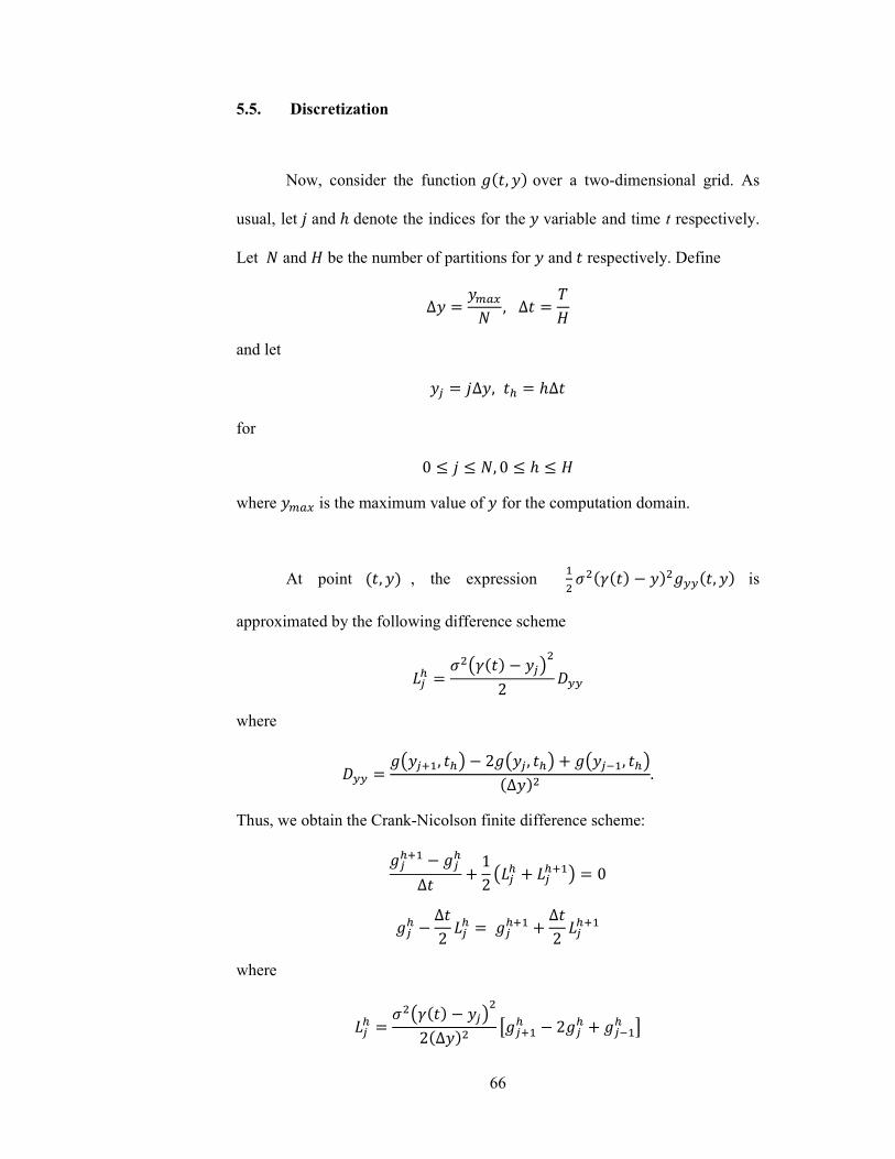
5.5. Discretization
Now, consider the function W, X over a two-dimensional grid. As
usual, let j and k denote the indices for the X variable and time t respectively.
Let l and m be the number of partitions for X and respectively. Define
∆X Xopql , ∆ m
and let
Xr j∆X, s k∆
for
0 j l, 0 k m
where Xopq is the maximum value of X for the computation domain.
At point , X , the expression @A A& XAW^^, X is
approximated by the following difference scheme
trs A+& Xr,A2 u^^
where
u^^ W+Xr4@, s, 2W+Xr, s, W+Xr*@, s,∆XA . Thus, we obtain the Crank-Nicolson finite difference scheme:
Wrs4@ Wrs∆ 12 +trs trs4@, 0
Wrs ∆2 trs Wrs4@ ∆2 trs4@
where
trs A+& Xr,A2∆XA 9Wr4@s 2Wrs Wr*@s <

67
and
trs4@ A+& ∆ Xr,A2∆XA 9Wr4@s4@ 2Wrs4@ Wr*@s4@<.
The finite difference scheme can be written as:
Wrs ∆A+& Xr,A4∆XA 9Wr4@s 2Wrs Wr*@s <
Wrs4@ ∆A+& ∆ Xr,A4∆XA 9Wr4@s4@ 2Wrs4@ Wr*@s4@<,
or
wrsWr*@s +1 2wrs,Wrs wrsWr4@s wrs4@Wr*@s4@ +1 2wrs4@,Wrs4@ wrs4@Wr4@s4@
After obtaining W, X , Asian call option value at time of the continuously
averaged with payoff at time is
x W !, '#.
5.6. Simulation and Analysis
The following tables present the result of Asian option values. The first table
compares the result using suggested method and Matlab build-in CRR
binomial tree method under different set of parameters, while the second table
shows the option values obtained by solving different dimensional of PDEs
using Crank-Nicolson method.

68
Table 5.1: Comparison of Crank-Nicolson finite difference scheme and CRR
Binomial Tree for pricing the Asian call option with K = 20 and Tmax = 1,
where Tmax is in year.
Crank-
Nicolson
CRR
Binomial
Tree
Relative
Error
Crank-
Nicolson
CRR
Binomial
Tree
Relative
Error
Crank-
Nicolson
CRR
Binomial
Tree
Relative
Error
0.05 0.25 1.3684 1.3702 1.27E-03 24.8625 24.8694 2.77E-04 78.5000 78.5208 2.65E-04
0.35 1.8064 1.8065 6.12E-05 24.8625 24.8694 2.77E-04 78.5000 78.5208 2.65E-04
0.4 2.0254 2.0247 3.35E-04 24.8626 24.8694 2.76E-04 78.5000 78.5208 2.65E-04
0.5 2.4625 2.4603 8.91E-04 24.8641 24.8706 2.62E-04 78.5000 78.5208 2.65E-04
0.65 3.1125 3.1089 1.15E-03 24.8859 24.8901 1.68E-04 78.5000 78.5208 2.65E-04
0.8 3.7245 3.7495 6.65E-03 24.9671 24.9669 8.31E-06 78.5000 78.5208 2.65E-04
0.1 0.25 1.6098 1.6061 2.28E-03 24.7275 24.7276 3.27E-06 77.0500 77.0745 3.18E-04
0.35 2.0195 2.0148 2.30E-03 24.7275 24.7276 3.23E-06 77.0500 77.0745 3.18E-04
0.4 2.2269 2.2217 2.34E-03 24.7275 24.7276 2.69E-06 77.0500 77.0745 3.18E-04
0.5 2.6433 2.6370 2.39E-03 24.7286 24.7284 7.50E-06 77.0500 77.0745 3.18E-04
0.65 3.2663 3.2589 2.30E-03 24.7460 24.7440 8.15E-05 77.0500 77.0745 3.18E-04
0.8 3.8640 3.8749 2.82E-03 24.8153 24.8096 2.28E-04 77.0500 77.0745 3.18E-04
0.15 0.25 1.8582 1.8548 1.82E-03 24.5700 24.5755 2.25E-04 75.6500 75.6605 1.39E-04
0.35 2.2337 2.2296 1.84E-03 24.5700 24.5755 2.25E-04 75.6500 75.6605 1.39E-04
0.4 2.4277 2.4232 1.88E-03 24.5700 24.5755 2.25E-04 75.6500 75.6605 1.39E-04
0.5 2.8211 2.8155 1.96E-03 24.5708 24.5761 2.17E-04 75.6500 75.6605 1.39E-04
0.65 3.4150 3.4083 1.97E-03 24.5847 24.5885 1.55E-04 75.6500 75.6605 1.39E-04
0.8 3.9936 3.9986 1.25E-03 24.6438 24.6443 2.24E-05 75.7000 75.6605 5.21E-04
r sigma
S0 = K = 20 S0 = 45 S0 = 100

69
Table 5.2: Comparison of Asian call option value by solving one-dimensional
and two-dimensional partial differential equation(PDE) using Crank-Nicolson
Scheme with K = 20 and Tmax = 1, where Tmax is in year.
One -
Dimensional
PDE
Two -
Dimensional
PDE
One -
Dimensional
PDE
Two -
Dimensional
PDE
One -
Dimensional
PDE
Two -
Dimensional
PDE
0.05 0.25 1.3684 1.3938 24.8625 24.8689 78.5000 78.5166
0.35 1.8064 1.8253 24.8625 24.8689 78.5000 78.5166
0.4 2.0254 2.0422 24.8626 24.8690 78.5000 78.5166
0.5 2.4625 2.4762 24.8641 24.8707 78.5000 78.5166
0.65 3.1125 3.1241 24.8859 24.8933 78.5000 78.5166
0.8 3.7245 3.7649 24.9671 24.9757 78.5000 78.5166
0.1 0.25 1.6098 1.6281 24.7275 24.7264 77.0500 77.0622
0.35 2.0195 2.0329 24.7275 24.7264 77.0500 77.0658
0.4 2.2269 2.2387 24.7275 24.7265 77.0500 77.0658
0.5 2.6433 2.6526 24.7286 24.7277 77.0500 77.0658
0.65 3.2663 3.2737 24.7460 24.7458 77.0500 77.0658
0.8 3.8640 3.8899 24.8153 24.8162 77.0500 77.0659
0.15 0.25 1.8582 1.8748 24.5700 24.5735 75.6500 75.6472
0.35 2.2337 2.2469 24.5700 24.5735 75.6500 75.6472
0.4 2.4277 2.4395 24.5700 24.5735 75.6500 75.6472
0.5 2.8211 2.8307 24.5708 24.5743 75.6500 75.6472
0.65 3.4150 3.4227 24.5847 24.5888 75.6500 75.6472
0.8 3.9936 4.0131 24.6438 24.6489 75.7000 75.6472
r sigma
S0 = K = 20 S0 = 45 S0 = 100
5.7. Conclusion
The Crank-Nicolson scheme used here has a very simple form and the results
obtained are close to the CRR binomial tree method.

70
CHAPTER 6
CONCLUSION
In this thesis, we apply Crank-Nicolson finite difference scheme to find option
value. An abundance literature of numerical option pricing is available in
various places, but one with systematic approach is rare to find. In chapter 4,
we obtain the value of Asian option by solving an initial value problem of a
two-dimensional Black-Scholes equation using a simple Crank-Nicolson finite
difference scheme. In chapter 5, we solve the same problem again by reducing
it to the solution of a one-dimensional equation applying a Change of
Argument due to Jan Večeř [13]. In these two chapters, we
develop a complete and systemic treatment for the solution.
Since we are solving an initial value problem in an unbounded domain, for
numerical computation, we have to truncate the unbounded domain into a
bounded domain and provide suitable boundary conditions through financial
or probabilistic consideration. Currently, we only have asymptotic boundary
conditions for large value of stock price. We have difficulty to determine a
stock price which is large enough that the boundary conditions are satisfied
with high accuracy. Thus our work here is partially based on trial and error.
Codes in Matlab are written to test our difference schemes. They are workable
and relatively accurate as compared to other methods [Chapter 4, pg 57].
However theoretical works of the effect of boundary conditions on the
solution should be studied in the future. Perhaps, we also can try to impose an

71
artificial boundary condition suggested by Han and Wu and Wong and Zhao
[22].
As Crank-Nicolson Scheme for the Black-Scholes equation involves a lot of
computations, stability analysis were carried out to ensure our result is stable
in section 4.7.
The problem of Asian options pricing is closely related to the integral of
geometric Brownian motion (called IGBM in the sequel). Indeed, it is
essentially a problem about exponential functionals of Brownian motion. In
several papers, Marc Yor [23,24] applied the properties of Bessel processes to
study the integral of geometric Brownian motion and obtained some of the
most important results about pricing of Asian options, in particular the
Geman-Yor formula [23,24] for the Laplace transform of Asian option prices
and the four known expressions for the probability density function (PDF in
the sequel) of IGBM. It will be interesting to know if an exponential
functional of Brownian motion will satisfy a simple heat equation through a
Change of Argument as presented here, for then our simple
Crank-Nicolson Scheme here is able to solve the highly complicated problem
of exponential functional of Brownian motion.

72
References
[1] A. Etheridge, A Course in Financial Calculus, New York: Cambridge
University Press, 2002.
[2] J.C. Hull, Options, Futures, and Other Derivatives, Fourth Edition,
Prentice Hall, New Jersey, 2000.
[3] S. E. Shreve, Stochastic Calculus for Finance II: Continuous-Time
Models, SpringerVerlag, New York, 2004.
[4] H. Geman, M. Yor, “Bessel processes, Asian option, and perpetuities”,
Mathematical Finance, vol. 3, pp. 349–375, 1993.
[5] M. Fu, D. Madan, T. Wang, “Pricing continuous Asian options: a
comparison of Monte Carlo and Laplace transform inversion methods”,
The Journal of Computational Finance, vol. 2, no. 2, 1998.
[6] V. Linetsky, “Exact Pricing of Asian Options: An Application of
Spectral Theory”, Working Paper, 2002.
[7] P. Boyle, D. Emanuel, “Options on the general mean”, Working paper,
1980.
[8] P. Boyle, M. Broadie, P. Glasserman, “Monte Carlo methods for
security pricing”, J. Econom. Dynam. Control, vol. 21, pp. 1267–1321,

73
1997.
[9] A. Kemna, A. Vorst, "A pricing method for options based on average
values". J. Banking Finance, vol. 14, pp. 113–129, 1997.
[10] L. Rogers, Z. Shi, “The value of an Asian option”, Journal of Applied
Probability, vol. 32, pp. 1077–1088, 1995.
[11] R. Zvan, P. Forsyth, K. Vetzal., “Robust numerical methods for PDE
models of Asian options”, The Journal of Computational Finance, vol.
1, no. 2, pp. 39–78, 1997.
[12] J. Večeř, “A new PDE approach for pricing arithmetic average Asian
options”, The Journal of Computational Finance, vol. 4, no. 4, pp.
105–113, 2001.
[13] J. Večeř, "Unified Pricing of Asian Options," Risk, June 2002.
[14] J. Večeř and M. Xu “Pricing Asian options in a semi martingale
model”, Quant. Fin. vol. 4, pp. 170-175, 2004.
[15] M. Broadie, P. Glasserman, S. Kou., “Connecting discrete and
continuous path dependent options”, Finance and Stochastics, vol. 3,
pp. 55–82, 1999.
[16] J. Ingersoll, “Theory of Financial Decision Making”, Oxford, 1987.

74
[17] J. Andreasen, “The pricing of discretely sampled Asian and lookback
options: a change of numeraire approach”, The Journal of
Computational Finance, vol. 2, no. 1, pp. 5–30, 1998.
[18] Y.K. Kwok, H.Y. Wong and K.W Lau, “Pricing algorithms of
multivariate path dependent options”, Journal of Complexity, vol. 17,
pp. 773-794, 2001.
[19] Eugene Isaacson and Herbert Bishop Keller, Analysis of Numerical
Methods. New York: Wiley, 1994.
[20] Y.K. Kwok, “Lattice tree methods for strongly path dependent
options”, Encyclopedia of Quantitative Finance, United Kingdom:
John Wiley and Sons Ltd, pp. 1022-1027, 2010.
[21] R. Kangro and R. Nicolaides, “Far field boundary conditions for
Black-Scholes equation”, SIAM Journal on Numerical Analysis, vol.
38(4), pp. 1357-1368, 2000.
[22] H.Y. Wong and J. Zhao, “An artificial boundary method for American
option pricing under CEV model”, SIAM Journal on Numerical
Analysis, vol. 46(4), pp. 2183-2209, 2008.
[23] M. Yor. “On some exponential functionals of Brownian motion,” Adv.
Appl. Prob., vol 24, pp. 509-531, 1992.

75
[24] M. Yor. “Exponential Functionals of Brownian Motion and Related
Processes,” Springer-Verlag, NewYork, 2001.
76
APPENDIX A
CODE FOR PRICING EUROPEAN OPTION
function [StkPrice Call SpPrice RelErr] =
EuropeanOption(K, r, sigma)
% Terminal time. Time unit in year
T = 1;
% Maximum stock price
Smax = 800;
% Compute the number of steps in stock price
% number of time step
H = 500;
% increment of time step
dt = 1/H;
% increment of stock price for each step
dS = sqrt(50*dt);
% number of step in Stock price
M = round(Smax/dS);
% The axis of stock price
s = dS : dS : Smax;
% Set the last interior stk price
M1 = M - 1;
% p(i,j) = Option Price at time i*dt(i=1..H); stk
price j*dS(j=1..M-1)
% left bdy value automatically taken care of during
initialization
% right bdy value at Smax = Smax - K*exp(-r(T-t));
% initialize p
p = zeros(H+1,M1);
% p(H+1,j) is the payoff at terminal time T when stk
price is j*dS
% P(1,j) is the payoff at time = 0

77
% Top Boundary
for j= 1 : M1
p(H+1,j) = max(s(j)-K,0);
end
% Define coefficients of difference equation:
% a(j)p(i-1,j-1) + b(j)p(i-1,j) + c(j)p(i-1,j+1) =
a1(j)p(i,j-1)+b1(j)p(i,j)+c1(j)p(i,j+1);
% Here i for time, j for stk price at time i
% b(j) at diagonal,a(j) to the left and c(j) to the
right
for j=1:M1
a(j)=dt/4*(r*j-sigma^2*j^2);
b(j)=1+dt*(r/2+1/2*sigma^2*j^2);
c(j)=-dt/4*(r*j+sigma^2*j^2);
end
for j=1:M1
a1(j) = -a(j);
b1(j) = 1 - dt/2*(sigma^2*j^2 + r);
c1(j) = -c(j);
end
% Construct coefficients matrices A and B
% where Ap(i-1,:) + down bdyValue(i-1) = Bp(i,:) +
up bdyValue(i)
A = zeros(M1,M1);
B = zeros(M1,M1);
% Put b(j) at diagonal, a(j) to left and c(j) to
right
for i = 1 : M1
j = i;
if i>1 A(i,j-1) = a(j); end
A(i,j) = b(j);
if j<M1 A(i,j+1) = c(j); end;
end
for i = 1 : M1
j = i;
if i>1 B(i,j-1) = a1(j); end
B(i,j) = b1(j);
if j<M1 B(i,j+1) = c1(j); end;
end

78
% vd,vu bdy Value vector of option at smax,time down
and up respectively
vd=zeros(M1,1);
vu=zeros(M1,1);
% Find Option Price
for i = H : -1 : 1
timeu = (H+1-i)*dt;
timed = (H+1-i-1)*dt;
vd(M1) = c(M1)*(Smax -K*exp(-r*timed));
vu(M1) = c1(M1)*(Smax-K*exp(-r*timeu));
p(i,:) = inv(A)* (vu-vd+B*p(i+1,:)');
end
% Check
for i = 1 : M1
idS(i) = i;
end;
format short g
StkPrice = 10 : 5 : Smax;
SpPrice = spline(idS, p(1,:), StkPrice/dS);
[Call, Put] = blsprice(StkPrice, K, r, T, sigma);
RelErr = abs(Call - SpPrice)./Call;
['StkPrice ' 'Call ' 'SpPrice ' 'RelErr']
[StkPrice' Call' SpPrice' RelErr'];
figure,plot(StkPrice',Call,'b',StkPrice',SpPrice,'r'
),xlabel('Stock Price'),ylabel('Option Value')

79
APPENDIX B
CODE FOR PRICING ASIAN OPTION BY SOLVING A TWO-
DIMENSIONAL PDE
function [StkPrice CallPrice SpPrice RelErr] =
AsianOption(K, r, sigma)
Smax = 500; % maximum stock price
Tmax = 1; % terminal time in year
Zmax = K*Tmax; % maximum accumulation of stock
price
M = 1000; % number of partition for average
stock price
N = 1000; % number of partition for stock price
T = 100; % number of partition for time
dS = Smax/N; % increment of stock price for each
step
dZ = Zmax/M; % increment of average stock price
for each step
dt = Tmax/T; % increment of time for each step
ratio = dt/dZ;
ratio2 = dt/(dS)^2;
ratio3 = dZ/(dS)^2 ;
s = dS : dS : Smax; % The axis of stock price
z = dZ : dZ : Zmax; % The axis of average stock
price
tLine = 0 : dt : Tmax;
% p(i,j,k) for Option Price at time kdt, stk
price jdS, avg stk price idz
% Top Boundary
for i = 1 : M
for j = 1 : N-1
p(i,j,T+1)=max((i-1)*dZ/Tmax - K,0);
% Payoff of call Option
end
end

80
for j = 1 : N-1
a(j)=-dt/4*((sigma^2*(j)^2)-r*(j));
b(j)=1 + (dt/2)*(sigma^2*(j)^2+(j)*dS/dZ+r);
c(j)=-dt/4*(r*(j)+sigma^2*(j)^2);
end
for j = 1 : N-1
a1(j)=-dt/4*((-sigma^2*(j)^2)+r*(j));
b1(j)=1-dt/2*(sigma^2*(j)^2+(j)*dS/dZ+r);
c1(j)=dt/4*(sigma^2*(j)^2+r*(j));
end
A=zeros(N-1,N-1);B=zeros(N-1,N-1);
% Put b(j) at diagonal of A; a(j) to left and
c(j) to right
for i = 1:N-1
j=i;
if i>1 A(i,j-1)=a(j); end
A(i,j)=b(j);
if j<N-1 A(i,j+1)=c(j); end;
end
for i = 1:N-1
j=i;
if i>1 B(i,j-1)=a1(j); end
B(i,j)=b1(j);
if j<N-1 B(i,j+1)=c1(j); end;
end
vdL = zeros(N-1,1);
vuL = zeros(N-1,1);
vdR = zeros(N-1,1);
vuR = zeros(N-1,1);
vu = zeros(N-1,1);
vd = zeros(N-1,1);
vu1 = zeros(N-1,1);
vd1 = zeros(N-1,1);

81
format short
for k = T : -1 : 1
timeu = (T+1-k-1)*dt;
timed = (T+1-k)*dt;
for j = N-1 : -1 : 1
vd(j) = -(dt*j*dS/(2*dZ))*((exp(-
r*timed))*(Zmax/Tmax - K)+ ((j*dS)/(r*Tmax))*(1-
exp(-r*timed)));
vu(j) = (dt*j*dS/(2*dZ))*((exp(-
r*timeu))*(Zmax/Tmax - K)+ ((j*dS)/(r*Tmax))*(1-
exp(-r*timeu)));
end
for i = M-1
vdR(N-1)= c(N-1) * max((exp(-
r*timed))*(i*dZ/Tmax - K)+(Smax/r*Tmax)*(1-exp(-
r*timed)),0);
vuR(N-1)= c1(N-1) * max((exp(-
r*timeu))*(i*dZ/Tmax - K)+(Smax/r*Tmax)*(1-exp(-
r*timeu)),0);
vdL(N-1)= a(1)*((exp(-
r*timed))*max(i*dZ/Tmax - K,0));
vuL(N-1)= a1(1)*((exp(-
r*timeu))*max(i*dZ/Tmax - K,0));
p(M,:,k)=inv(A)*(vuL-vdL + vuR-vdR + vu-vd +
B*p(M,:,k+1)');
end
for i = M-2 : -1 : 0
vdR(N-1)= c(N-1) * max((exp(-
r*timed))*(i*dZ/Tmax - K)+(Smax/r*Tmax)*(1-exp(-
r*timed)),0); % OK
vuR(N-1)= c1(N-1) * max((exp(-
r*timeu))*(i*dZ/Tmax - K)+(Smax/r*Tmax)*(1-exp(-
r*timeu)),0);% OK
vdL(N-1)= a(1)*((exp(-
r*timed))*max(i*dZ/Tmax - K,0)); % OK
vuL(N-1)= a1(1)*((exp(-
r*timeu))*max(i*dZ/Tmax - K,0)); % OK
for j = N-1 : -1 : 1
vu1(j) = (dt*j*dS/(2*dZ))*p(i+2,j,k+1)';

82
vd1(j) = -(dt*j*dS/(2*dZ))*p(i+2,j,k)';
end
p(i+1,:,k)=inv(A)*(vuL-vdL + vuR-vdR + vu1-
vd1 + B*p(i+1,:,k+1)');
end
end
CN=p(1,:,1);
% Check
for i=1:N-1
idS(i)=i;
end;
format long g
StkPrice = 10 : 5 : Smax;
size = length(StkPrice);
SpPrice = spline(idS,CN,StkPrice/dS);
for i = 1 : size
StockSpec(i) = stockspec(sigma, StkPrice(i));
RateSpec = intenvset('Rates', r,
'StartDates','1-Jan-2004', 'EndDates', '31-Dec-
2004','Compounding',-1);
ValuationDate = '1-Jan-2004';
Maturity = '31-Dec-2004';
TimeSpec = crrtimespec(ValuationDate, Maturity,
100);
CRRTree(i) = crrtree(StockSpec(i), RateSpec,
TimeSpec);
OptSpec = 'call';
Strike = K;
Settle = '01-Jan-2004';
ExerciseDates = '31-Dec-2004';
CallPrice(i) = asianbycrr(CRRTree(i), OptSpec,
Strike, Settle, ExerciseDates);
end

83
RelErr = abs(CallPrice-SpPrice)./CallPrice;
['StkPrice ' 'Simulation ' 'CN ' 'RelErr']
[StkPrice' CallPrice' SpPrice' RelErr'];
figure,plot(StkPrice,CallPrice,'b',StkPrice,SpPrice,
'r'),xlabel('Stock Price'),ylabel('Option Value')

84
APPENDIX C
CODE FOR PRICING ASIAN OPTION BY SOLVING A ONE –
DIMENSIONAL PDE
Code for pricing Asian Option by Solving a One-Dimensional PDE
function [y, g, S0] = AsianTransform(S0, K, r, sigma)
Tmax = 1; % Set the terminal time. Time unit in year
Ymax = 1; % set the Max Y value
Ymin = -Ymax;
X0 = (S0/(r*Tmax))*(1-exp(-r*Tmax)) - K*exp(-r*Tmax);
Y0 = X0/S0;
H = 2000; % number of time step
Y = 2000; % number of Y step
dt = Tmax/H; % increment of time step
dY = Ymax/Y; % increment of Y step
t = dt : dt : Tmax;
y = Ymin : dY : Ymax;
N = size(y,2);
% Number of holding shares
for h = 1 : H
Q(h) = ((1/r*Tmax)*(1-exp(-r*(Tmax - (h-
1)*dt))));
end
% Calculate the coefficient
for h = 1 : H
for j = 1:N
alpha(h,j) = (dt*(sigma^2)*(Q(h)-
(y(j)))^2)/(4*((dY)^2));
end
end
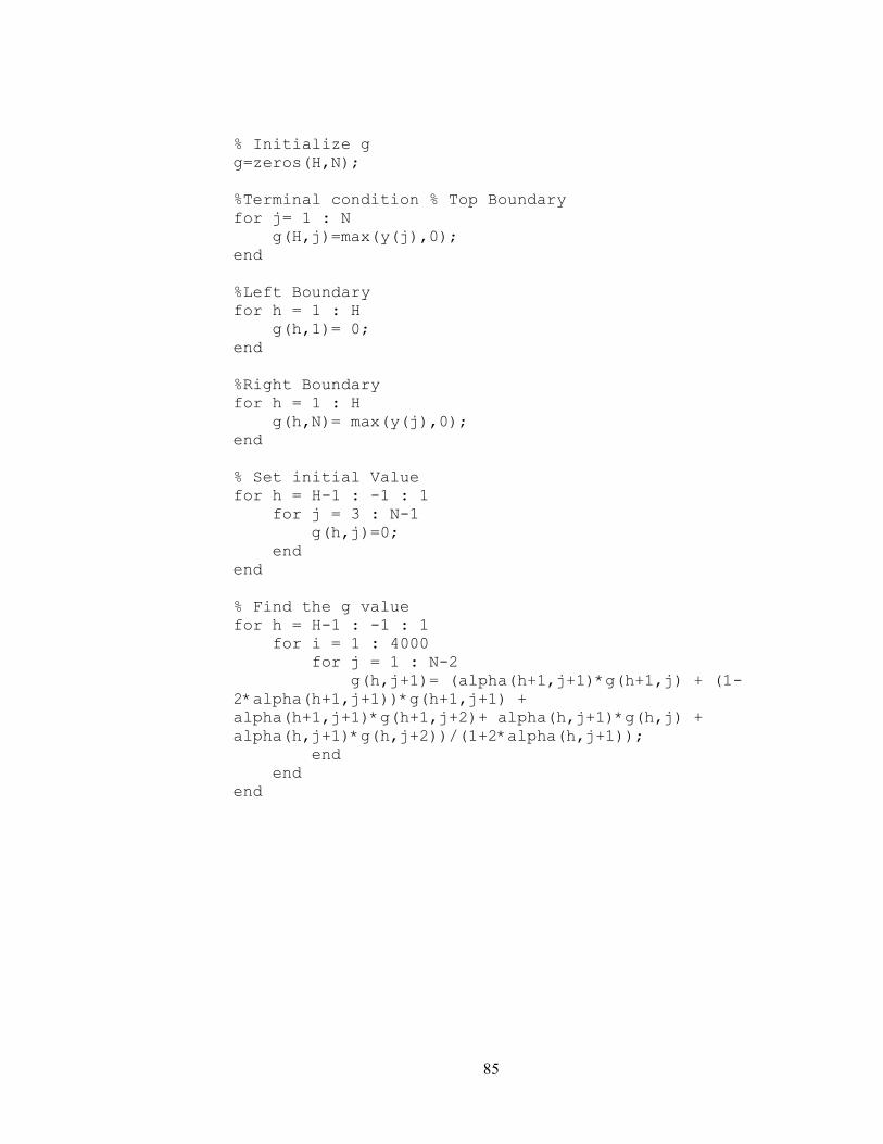
85
% Initialize g
g=zeros(H,N);
%Terminal condition % Top Boundary
for j= 1 : N
g(H,j)=max(y(j),0);
end
%Left Boundary
for h = 1 : H
g(h,1)= 0;
end
%Right Boundary
for h = 1 : H
g(h,N)= max(y(j),0);
end
% Set initial Value
for h = H-1 : -1 : 1
for j = 3 : N-1
g(h,j)=0;
end
end
% Find the g value
for h = H-1 : -1 : 1
for i = 1 : 4000
for j = 1 : N-2
g(h,j+1)= (alpha(h+1,j+1)*g(h+1,j) + (1-
2*alpha(h+1,j+1))*g(h+1,j+1) +
alpha(h+1,j+1)*g(h+1,j+2)+ alpha(h,j+1)*g(h,j) +
alpha(h,j+1)*g(h,j+2))/(1+2*alpha(h,j+1));
end
end
end
Top Related