


Languages
Pages
Legal

COVERAGE-DRIVEN TEST GENERATION FOR FUNCTIONAL VALIDATION OFPIPELINED PROCESSORS
By
HEON-MO KOO
A DISSERTATION PRESENTED TO THE GRADUATE SCHOOLOF THE UNIVERSITY OF FLORIDA IN PARTIAL FULFILLMENT
OF THE REQUIREMENTS FOR THE DEGREE OFDOCTOR OF PHILOSOPHY
UNIVERSITY OF FLORIDA
2007
1

c© 2007 Heon-Mo Koo
2

To my wife Jungmin Shin, daughter Jimin Koo, father Bonkyoung Koo, and mother
Okryon Lee for their love and encouragement
3

ACKNOWLEDGMENTS
My journey to the Ph.D. was full of challenging adventures and it became another
stepping-stone in my life. Though only my name appears on the cover of this dissertation,
the completion of my dissertation was possible with the help and efforts of many people.
First, I express my deepest appreciation to my esteemed advisor Dr. Prabhat Mishra.
Through my graduate career at University of Florida, his unfailing guidance, support,
and patience helped me overcome many crisis situations and complete this dissertation.
He often brought me to the threshold of knowledge, and ignited the interest to cross the
threshold. He also encouraged me to be an independent thinker with a high research
standard. Additionally, I am very grateful for the friendship of all of the members of his
research group.
Thanks also go out to the members of the dissertation committee, Profs. Sartaj
Sahni, Jih-Kwon Peir, Shigang Chen, and John M. Shea for their valuable suggestions.
Their insightful comments and constructive criticisms were thought-provoking and helped
my idea escalate at each phase of my research.
I am grateful to many people on the faculty and staff of the Department of Computer
and Information Science and Engineering for all that they taught and supported me in
various ways. I am also thankful to the students who I was privileged to teach and from
whom I also learned much when I was a Teaching Assistant.
Finally, and most importantly, I sincerely thank my family who have been a constant
source of help, support, and strength during doctoral studies. None of my achievement
would have been possible without their love. My very special thanks to my wife for her
unselfish devotion and love upon which the path to completing my Ph.D. was built.
I warmly appreciate my parents for their unwavering faith in me as well as unending
encouragement and support. I thank my brother and sisters for their love and support. I
appreciate parents-in-law for consistent encouragement and support.
4

TABLE OF CONTENTS
page
ACKNOWLEDGMENTS . . . . . . . . . . . . . . . . . . . . . . . . . . . . . . . . . 4
LIST OF TABLES . . . . . . . . . . . . . . . . . . . . . . . . . . . . . . . . . . . . . 7
LIST OF FIGURES . . . . . . . . . . . . . . . . . . . . . . . . . . . . . . . . . . . . 8
ABSTRACT . . . . . . . . . . . . . . . . . . . . . . . . . . . . . . . . . . . . . . . . 9
CHAPTER
1 INTRODUCTION . . . . . . . . . . . . . . . . . . . . . . . . . . . . . . . . . . 10
1.1 Processor Validation . . . . . . . . . . . . . . . . . . . . . . . . . . . . . . 121.2 Coverage-driven Functional Validation . . . . . . . . . . . . . . . . . . . . 141.3 Research Contributions . . . . . . . . . . . . . . . . . . . . . . . . . . . . . 16
2 PROCESSOR FAULT MODELING AND FUNCTIONAL COVERAGE . . . . 19
2.1 Existing Fault Models and Coverage Metrics . . . . . . . . . . . . . . . . . 192.1.1 Fault Models . . . . . . . . . . . . . . . . . . . . . . . . . . . . . . . 192.1.2 Coverage Metrics . . . . . . . . . . . . . . . . . . . . . . . . . . . . 20
2.2 Graph-based Modeling of Pipelined Processors . . . . . . . . . . . . . . . . 232.2.1 Modeling of MIPS processor . . . . . . . . . . . . . . . . . . . . . . 242.2.2 Modeling of PowerPC e500 processor . . . . . . . . . . . . . . . . . 25
2.3 Pipeline Interaction Fault Model and Functional Coverage . . . . . . . . . 262.4 Chapter Summary . . . . . . . . . . . . . . . . . . . . . . . . . . . . . . . 28
3 TEST GENERATION USING DESIGN AND PROPERTYDECOMPOSITIONS . . . . . . . . . . . . . . . . . . . . . . . . . . . . . . . . . 29
3.1 Model Checking . . . . . . . . . . . . . . . . . . . . . . . . . . . . . . . . 303.2 Test Generation using Model Checking . . . . . . . . . . . . . . . . . . . . 323.3 Related Work . . . . . . . . . . . . . . . . . . . . . . . . . . . . . . . . . . 343.4 Test Generation using Design and Property Decompositions . . . . . . . . 36
3.4.1 Generation and Negation of Properties . . . . . . . . . . . . . . . . 383.4.2 Property Decomposition . . . . . . . . . . . . . . . . . . . . . . . . 38
3.4.2.1 Decomposable properties . . . . . . . . . . . . . . . . . . . 393.4.2.2 Non-decomposable properties . . . . . . . . . . . . . . . . 40
3.4.3 Design Decomposition . . . . . . . . . . . . . . . . . . . . . . . . . . 433.4.4 Test Generation using Decompositional Model Checking . . . . . . . 443.4.5 Merging Partial Counterexamples . . . . . . . . . . . . . . . . . . . 51
3.5 Experiments . . . . . . . . . . . . . . . . . . . . . . . . . . . . . . . . . . . 523.5.1 Test Generation using Module Level Decomposition . . . . . . . . . 523.5.2 Test Generation for e500 Processor . . . . . . . . . . . . . . . . . . 54
5

3.5.2.1 Results . . . . . . . . . . . . . . . . . . . . . . . . . . . . 543.5.2.2 Micro-architectural validation using test programs . . . . 54
3.6 Chapter Summary . . . . . . . . . . . . . . . . . . . . . . . . . . . . . . . 57
4 TEST GENERATION USING SAT-BASED BOUNDED MODEL CHECKING 58
4.1 SAT-based Bounded Model Checking . . . . . . . . . . . . . . . . . . . . . 594.2 Related Work . . . . . . . . . . . . . . . . . . . . . . . . . . . . . . . . . . 614.3 Test Generation using SAT-based Bounded Model Checking . . . . . . . . 61
4.3.1 Determination of Bound . . . . . . . . . . . . . . . . . . . . . . . . 634.3.2 Design and Property Decompositions . . . . . . . . . . . . . . . . . 64
4.4 A Case Study . . . . . . . . . . . . . . . . . . . . . . . . . . . . . . . . . . 644.4.1 Experimental Setup . . . . . . . . . . . . . . . . . . . . . . . . . . 654.4.2 Test Generation: An Example . . . . . . . . . . . . . . . . . . . . . 654.4.3 Results . . . . . . . . . . . . . . . . . . . . . . . . . . . . . . . . . 66
4.5 Chapter Summary . . . . . . . . . . . . . . . . . . . . . . . . . . . . . . . 68
5 FUNCTIONAL TEST COMPACTION . . . . . . . . . . . . . . . . . . . . . . . 69
5.1 Related Work . . . . . . . . . . . . . . . . . . . . . . . . . . . . . . . . . . 705.2 FSM Modeling . . . . . . . . . . . . . . . . . . . . . . . . . . . . . . . . . 71
5.2.1 Functional FSM Modeling of Processors . . . . . . . . . . . . . . . . 725.2.1.1 Modeling of FSM states . . . . . . . . . . . . . . . . . . . 725.2.1.2 Modeling of FSM state transitions . . . . . . . . . . . . . 73
5.2.2 Functional Coverage of FSM Model . . . . . . . . . . . . . . . . . . 755.3 Compaction before Test Generation . . . . . . . . . . . . . . . . . . . . . . 76
5.3.1 Identifying Unreachable States . . . . . . . . . . . . . . . . . . . . . 765.3.2 Identifying Redundant States and Transitions . . . . . . . . . . . . 775.3.3 Identifying Illegal State Transitions . . . . . . . . . . . . . . . . . . 78
5.4 FSM Coverage-directed Test Generation . . . . . . . . . . . . . . . . . . . 795.4.1 Test Generation for State Coverage . . . . . . . . . . . . . . . . . . 795.4.2 Test Generation for Transition Coverage . . . . . . . . . . . . . . . 79
5.5 Compaction after Test Generation . . . . . . . . . . . . . . . . . . . . . . . 805.5.1 Test Matrix Reduction . . . . . . . . . . . . . . . . . . . . . . . . . 805.5.2 Test Set Minimization . . . . . . . . . . . . . . . . . . . . . . . . . . 81
5.6 Experiments . . . . . . . . . . . . . . . . . . . . . . . . . . . . . . . . . . 815.7 Chapter Summary . . . . . . . . . . . . . . . . . . . . . . . . . . . . . . . 84
6 CONCLUSIONS AND FUTURE WORK . . . . . . . . . . . . . . . . . . . . . 85
6.1 Conclusions . . . . . . . . . . . . . . . . . . . . . . . . . . . . . . . . . . . 856.2 Future Research Directions . . . . . . . . . . . . . . . . . . . . . . . . . . . 86
REFERENCES . . . . . . . . . . . . . . . . . . . . . . . . . . . . . . . . . . . . . . . 87
BIOGRAPHICAL SKETCH . . . . . . . . . . . . . . . . . . . . . . . . . . . . . . . . 96
6

LIST OF TABLES
Table page
2-1 Code coverage metrics . . . . . . . . . . . . . . . . . . . . . . . . . . . . . . . . 21
2-2 FSM coverage metrics . . . . . . . . . . . . . . . . . . . . . . . . . . . . . . . . 22
3-1 Design and property decomposition scenarios . . . . . . . . . . . . . . . . . . . 37
3-2 Comparison of test generation techniques . . . . . . . . . . . . . . . . . . . . . . 53
3-3 Various test cases generated by our framework . . . . . . . . . . . . . . . . . . . 55
4-1 Example of a test program . . . . . . . . . . . . . . . . . . . . . . . . . . . . . . 65
4-2 Comparison of test generation techniques for pipeline interactions . . . . . . . . 66
5-1 Transition rules between ssk,j−1(t− 1) and ssi,j(t) . . . . . . . . . . . . . . . . . 78
5-2 Transition rules between ssi,j(t− 1) and ssi,j(t) . . . . . . . . . . . . . . . . . . 78
5-3 Transition rules between ssl,j+1(t− 1) and ssi,j(t) . . . . . . . . . . . . . . . . . 78
7

LIST OF FIGURES
Figure page
1-1 Pre-silicon logic bugs per generation . . . . . . . . . . . . . . . . . . . . . . . . 11
1-2 Simulation-based processor validation . . . . . . . . . . . . . . . . . . . . . . . . 13
1-3 Coverage-driven validation flow . . . . . . . . . . . . . . . . . . . . . . . . . . . 15
1-4 Functional coverage-directed test generation methodology . . . . . . . . . . . . . 17
2-1 Graph model of the MIPS processor . . . . . . . . . . . . . . . . . . . . . . . . 24
2-2 Instruction flow of the PowerPC e500 processor . . . . . . . . . . . . . . . . . . 25
3-1 Test generation methodology using design and property decompositions . . . . . 29
3-2 Test generation using model checking . . . . . . . . . . . . . . . . . . . . . . . . 32
3-3 Specification-driven test generation using model checking . . . . . . . . . . . . . 33
3-4 An example of Kripke structure model . . . . . . . . . . . . . . . . . . . . . . . 42
3-5 Four different data forwarding mechanisms . . . . . . . . . . . . . . . . . . . . . 55
3-6 Micro-architectural validation flow . . . . . . . . . . . . . . . . . . . . . . . . . 56
4-1 Test program generation using SAT-based bounded model checking . . . . . . . 59
4-2 Test generation time comparison for four techniques . . . . . . . . . . . . . . . . 67
5-1 Functional test compaction methodology . . . . . . . . . . . . . . . . . . . . . . 70
5-2 Binary format of the states in FSM model . . . . . . . . . . . . . . . . . . . . . 73
5-3 Instruction flow . . . . . . . . . . . . . . . . . . . . . . . . . . . . . . . . . . . . 74
5-4 Pipeline interactions . . . . . . . . . . . . . . . . . . . . . . . . . . . . . . . . . 74
5-5 Single transitions between neighboring states . . . . . . . . . . . . . . . . . . . . 77
5-6 Test matrix for FSM coverage . . . . . . . . . . . . . . . . . . . . . . . . . . . . 81
5-7 Simplified MIPS processor . . . . . . . . . . . . . . . . . . . . . . . . . . . . . . 82
5-8 7-bits functional FSM model . . . . . . . . . . . . . . . . . . . . . . . . . . . . . 82
8

Abstract of Dissertation Presented to the Graduate Schoolof the University of Florida in Partial Fulfillment of theRequirements for the Degree of Doctor of Philosophy
COVERAGE-DRIVEN TEST GENERATION FOR FUNCTIONAL VALIDATION OFPIPELINED PROCESSORS
By
Heon-Mo Koo
December 2007
Chair: Prabhat MishraMajor: Computer Engineering
Functional verification of microprocessors is one of the most complex and expensive
tasks in the current system-on-chip design methodology. Simulation using functional
test vectors is the most widely used form of processor verification. A major challenge in
simulation-based verification is how to reduce the overall verification time and resources.
Traditionally, billions of random and directed tests are used during simulation. Compared
to random tests, directed tests can reduce overall validation effort significantly since
shorter tests can obtain the same coverage goal. However, there is a lack of automated
techniques for directed test generation targeting micro-architectural design errors.
Furthermore, the lack of a comprehensive functional coverage metric makes it difficult to
measure the verification progress. This dissertation presents a functional coverage-driven
test generation methodology. Based on the behavior of pipelined processors, a functional
coverage is defined to evaluate the verification progress. My research provides efficient
test generation techniques using formal methods by decomposing processor designs and
properties to reduce test generation time as well as memory requirement. My research
also provides a functional test compaction technique to reduce the number of directed
tests while preserving the overall functional coverage. The experiments using MIPS and
PowerPC processors demonstrate the feasibility and usefulness of the proposed functional
test generation methodology.
9
CHAPTER 1INTRODUCTION
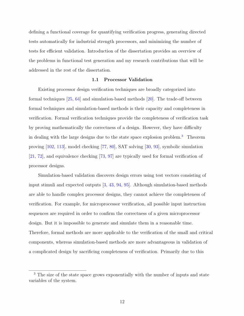
Verification is the process of ensuring that the intent of a design is preserved in
its implementation. Functional verification (or validation1 ) can expose functional logic
errors in the hardware designs which are described in behavioral model, register transfer
level model, gate level model, or switch level model. Functional errors are introduced
due to various factors including careless coding, misinterpretation of the specification,
microarchtectural design complexity, corner cases, and so on. If any functional bug is
found in a chip already fabricated, the error needs to be corrected and the modified
version of the design needs to be fabricated again, which is very expensive. In the worst
case, bug fixing after delivery to customers will entail a very costly replacement as well as
re-fabrication expenses. For example, in 1994 Intel’s Pentium processor had a functional
error called FDIV bug2 and the company had to spend a staggering cost to replace the
faulty processors.
In modern microprocessor designs, functional verification is one of the major
bottlenecks due to the combined effects of increasing design complexity and decreasing
time-to-market. Design complexity of modern processors is increasing at an alarming
rate to cope up with the required performance improvement for increasingly complex
applications in the domains of communication, multimedia, networking and entertainment.
To accommodate such faster computation requirements, today’s processors employ many
complicated micro-architectural features such as deep pipelines, dynamic scheduling,
out-of-order and superscalar execution, and dynamic speculation. This trend again shows
1 The term “validation” is generally used for simulation-based approaches, while“verification” is used for both simulation-based and formal methods.
2 The Pentium FDIV bug was the most infamous of the Intel microprocessor bugs. Dueto an error in a lookup table, certain floating point division operations would produceincorrect results.
10
Pentium Pentium Pro Pentium 4 Next ?
8002240
7855
25000
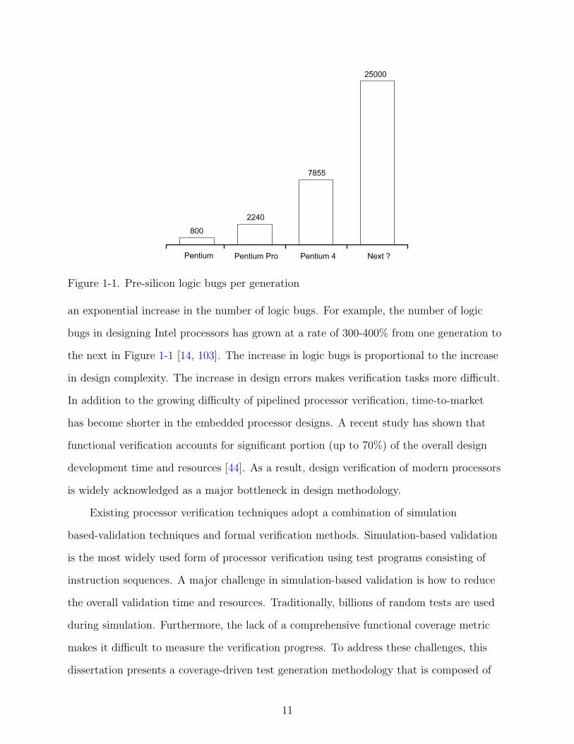
Figure 1-1. Pre-silicon logic bugs per generation
an exponential increase in the number of logic bugs. For example, the number of logic
bugs in designing Intel processors has grown at a rate of 300-400% from one generation to
the next in Figure 1-1 [14, 103]. The increase in logic bugs is proportional to the increase
in design complexity. The increase in design errors makes verification tasks more difficult.
In addition to the growing difficulty of pipelined processor verification, time-to-market
has become shorter in the embedded processor designs. A recent study has shown that
functional verification accounts for significant portion (up to 70%) of the overall design
development time and resources [44]. As a result, design verification of modern processors
is widely acknowledged as a major bottleneck in design methodology.
Existing processor verification techniques adopt a combination of simulation
based-validation techniques and formal verification methods. Simulation-based validation
is the most widely used form of processor verification using test programs consisting of
instruction sequences. A major challenge in simulation-based validation is how to reduce
the overall validation time and resources. Traditionally, billions of random tests are used
during simulation. Furthermore, the lack of a comprehensive functional coverage metric
makes it difficult to measure the verification progress. To address these challenges, this
dissertation presents a coverage-driven test generation methodology that is composed of
11
defining a functional coverage for quantifying verification progress, generating directed
tests automatically for industrial strength processors, and minimizing the number of
tests for efficient validation. Introduction of the dissertation provides an overview of
the problems in functional test generation and my research contributions that will be
addressed in the rest of the dissertation.
1.1 Processor Validation
Existing processor design verification techniques are broadly categorized into
formal techniques [25, 64] and simulation-based methods [20]. The trade-off between
formal techniques and simulation-based methods is their capacity and completeness in
verification. Formal verification techniques provide the completeness of verification task
by proving mathematically the correctness of a design. However, they have difficulty
in dealing with the large designs due to the state space explosion problem.3 Theorem
proving [102, 113], model checking [77, 80], SAT solving [30, 93], symbolic simulation
[21, 72], and equivalence checking [73, 97] are typically used for formal verification of
processor designs.
Simulation-based validation discovers design errors using test vectors consisting of
input stimuli and expected outputs [3, 43, 94, 95]. Although simulation-based methods
are able to handle complex processor designs, they cannot achieve the completeness of
verification. For example, for microprocessor verification, all possible input instruction
sequences are required in order to confirm the correctness of a given microprocessor
design. But it is impossible to generate and simulate them in a reasonable time.
Therefore, formal methods are more applicable to the verification of the small and critical
components, whereas simulation-based methods are more advantageous in validation of
a complicated design by sacrificing completeness of verification. Primarily due to this
3 The size of the state space grows exponentially with the number of inputs and statevariables of the system.
12

MOV R1, 011
MOV R2, 010
ADD R3, R1, R2
# R3 == 101
R3 == 101 ?
Design simulator
Test generator
Test Program
Fetch
Decode
PC
DIVFADD1IALU MUL1
FADD3
FADD2MUL2
FADD4
MEM
WriteBack
Register File
Memory
MUL7
Check Result
MOV R1, 011
MOV R2, 010
ADD R3, R1, R2
# R3 == 101
R3 == 101 ?
Design simulator
Test generator
Test Program
Fetch
Decode
PC
DIVFADD1IALU MUL1
FADD3
FADD2MUL2
FADD4
MEM
WriteBack
Register File
Memory
MUL7
Check Result
Figure 1-2. Simulation-based processor validation
reason, simulation-based validation is the most widely used form of verifying modern
complex processors.
The basic procedure in simulation-based processor validation consists of generating
test programs, simulating a given processor design with the test programs, comparing
the generated outputs with the expected results, and correcting design errors if the
simulation outputs are different from the expected results (Figure 1-2). A major challenge
in processor validation is how to reduce the overall validation time and resources. Since
the test generation and simulation for all input test programs is infeasible, we need a
method for deciding effective tests to achieve high confidence of the processor design. In
addition, test generation techniques must be able to accommodate complex processor
designs as well as produce tests in reasonable time. The main focus of this dissertation is
the functional test program generation for validation of pipelined processors.
13
There are three types of test generation techniques: random, constrained-random,
and directed. In the current industrial practice [2, 100], random and constrained-random
test generation techniques at architecture (ISA) level are most widely used because test
programs can be produced automatically and design errors can be uncovered early in the
design cycle. However, a huge number of tests are required to achieve high confidence of
the design correctness, and corner cases are easily missed. Furthermore, architectural test
generation techniques have difficulty in activating micro-architectural target artifacts and
pipeline functionalities since it is not possible to generate information regarding pipeline
interactions or timing details using input ISA specification.
Compared to the random or constrained-random tests, the directed tests can reduce
overall validation effort significantly since shorter tests can obtain the same functional
coverage goal. However, there is a lack of automated techniques for directed test
generation targeting micro-architectural faults. As a result, directed tests are typically
hand-written by experts. Due to manual development, it is infeasible to generate all
directed tests to achieve comprehensive coverage and this process is time consuming and
error prone. Therefore, there is a need for automated directed test generation techniques
based on micro-architectural functional coverage. Test generation using formal methods
has been successfully used due to its capability of automatic test generation. However,
the traditional test generation techniques are unsuitable for large designs due to the state
explosion problem. To address these challenges, my research provides automated test
generation techniques using decomposition of processor design and property to make the
formal methods applicable in practice.
1.2 Coverage-driven Functional Validation
A main drawback in simulation-based validation is that an assurance of the
correctness of the design requires exhaustive simulation which is possible only for small
designs. In other words, a certain degree of confidence can be achieved by simulating the
design using a large volume of tests. However, there is a lack of good metrics to quantify
14

Create coverage metric
Generate random testsor
Coverage directed tests
Run simulation
Collect coverage
Identify coverage holes
Add tests to target holes andenhance coverage metric, if needed
Create coverage metric
Generate random testsor
Coverage directed tests
Run simulation
Collect coverage
Identify coverage holes
Add tests to target holes andenhance coverage metric, if needed
Figure 1-3. Coverage-driven validation flow
this degree of confidence and to qualify a test set. Therefore, it is hard to answer the
question, “When is verification done?”, due to difficulty in measuring verification progress
and test effectiveness.
A traditional flow of coverage-driven validation begins by defining coverage metric,
followed by test generation (Figure 1-3). A coverage metric provides a way to see what
has not been verified and what tests should be added. Many coverage metrics have
been proposed for different types of design errors (e.g., control flow, data flow) and at
different design abstraction levels (e.g., behavioral, RTL, gate level). In coverage-driven
test generation, tests are created to activate a target coverage point and it can effectively
reduce the number of tests compared to the random test generation. Through simulation,
the coverage is analyzed by examining whether target functionalities have been covered
or not, thereby we can measure the validation progress. If coverage holes are found,
additional tests are generated to exercise them. If higher degree of confidence is required,
we can improve the coverage metric or make use of additional coverage measures.
Verification engineers can change the scope or depth of coverage during the validation
15

process. For example, they can start from simple coverage metrics in the early verification
stage and use more complex coverage metrics later on. However, existing coverage metrics
do not have a direct relationship with the design functionality, we need a coverage metric
based on the functionality of the design. This dissertation provides a comprehensive
functional coverage metric by defining a functional fault model for pipelined processors.
Although directed tests require a smaller test set compared to random tests for
the same functional coverage goal, the number of tests can still be extremely large.
Therefore, there is a need for functional test compaction techniques. My research provides
a functional test compaction technique to reduce the directed test set.
1.3 Research Contributions
The goal of my research is to provide an efficient functional test generation methodology
for validation of pipelined processors, thereby reducing overall validation efforts. Since
generating and simulating all possible instruction sequences is not possible for modern
processor verification, we need a method to decide an effective test set to achieve high
confidence of the design correctness. In addition, test generation techniques should be able
to handle complex processor designs and produce the tests in efficient way. Therefore, two
important things should be considered in test generation: (i) what tests to be generated
and (ii) how to create them. Moreover, compacting the test set without sacrificing
coverage goal is necessary to further reduce validation efforts.
Figure 1-4 shows the overall flow of the proposed coverage-driven functional test
generation methodology [66]. The first step is to create a processor model and a functional
fault model from the processor architecture specification. Next, it generates a list of
all possible functional faults based on the fault model and the processor model under
validation. Test compaction is performed before test generation by eliminating the
redundant faults for the given design constraints. One of the remaining faults is selected
for test generation. A test program for this fault is produced automatically by formal
verification methods, e.g., model checking. The fault is removed from the fault list. This
16

Processor model Functional fault model
Generate fault list
Select an undetected faultfor test generation
Generate a test programfor the fault using formal methods
Generate a list of other faultsdetected by the test program
Put the detected faults offof the fault list
Detect all faults?
Yes
No
Architecture Specification(English Document)
Test compaction
Test set
Test compaction
Figure 1-4. Functional coverage-directed test generation methodology
loop repeats until tests are generated for all the faults in the fault list. Functional test
compaction is performed after this flow of test generation. It is important to note that
two steps of compaction techniques are applied before and after test generation. This
dissertation makes three major contributions: i) development of efficient fault models
and a coverage metric for pipeline interaction functionalities, ii) novel test generation
techniques using formal methods for modern complex processor designs, and iii) functional
test compaction.
17

We define a pipeline interaction fault model using both graph and FSM-based
modeling of pipelined processors. The fault model is used to define a functional coverage.
The functional coverage is used to measure the validation progress by reporting the faults
that are covered by a given set of test programs.
This dissertation presents a unified methodology for automated test generation
using model checking and satisfiability (SAT) solving. To alleviate the state explosion
problem in the existing model checking-based test generation, we have developed efficient
test generation techniques that use design level as well as property level decompositions
to reduce test generation time and memory requirement. This dissertation presents
procedures for decomposing desired properties and processor model with an algorithm for
constructing test programs from partial counterexamples. Compared to traditional model
checking, SAT-based bounded model checking (BMC) is more efficient in generating
counterexamples if there exists a counterexample within search bound. However,
appropriate decision of the search space of tests is another challenging problem. This
dissertation also provides a procedure for determining the bound in the presence of design
and property decompositions. The dissertation shows the applicability of design and
property decompositions in the context of traditional model checking and SAT-based
BMC.
Development of a test compaction technique in the dissertation reduces the number of
directed tests without loss of functional coverage in an effort to further reduce the overall
validation effort. Even though the proposed test generation techniques require a much
smaller test set than random tests, the volume of a directed test set still remains huge.
Redundant properties are eliminated before test generation and test matrix reduction
techniques are applied after test generation. The efficient test generation and compaction
techniques in this dissertation will reduce the overall validation effort by several order of
magnitude.
18

CHAPTER 2PROCESSOR FAULT MODELING AND FUNCTIONAL COVERAGE
Coverage metrics are necessary to evaluate the progress of functional validation.
Several coverage metrics are commonly used during functional validation such as code
coverage, and state/transition coverage of abstract finite state machines (FSM). However,
these coverage metrics do not have a direct relationship with the design functionality. For
example, none of the existing coverage metrics determines if all possible interactions of
stalls are tested in a pipelined processor. Therefore, we need a coverage metric based on
the functionality of pipelined processors. In this chapter, a pipeline interaction fault model
is defined using graph-based modeling of pipelined processors. The fault model is used for
generating directed tests and defining the functional coverage to measure the validation
progress by reporting the faults that are covered by a given set of test programs.
2.1 Existing Fault Models and Coverage Metrics
The process of modeling design errors in the design hierarchy is called fault modeling
which is necessary to generate tests and analyze the result of the tests [1, 107]. A fault
model should be able to represent high percentage of actual errors. Moreover, it should be
as simple as possible to reduce complexity of test generation and coverage analysis. The
fault model can be used to define coverage metrics. For example, stuck-at fault model and
corresponding stuck-at fault coverage are used for manufacturing tests. This summarizes
existing work on functional fault models and coverage metrics.
2.1.1 Fault Models
Functional fault is a representation of an error at the abstracted functional level.
Since modeling of faults depends on modeling of design, fault models have been developed
at different levels of design abstraction, e.g., functional, structural (gate level), and
switch level [23, 62]. Functional fault models are defined at a high abstraction level
and functional faults correspond to incorrect execution of the functionalities against a
given specification. For example, in validation of microprocessor designs, an instruction
19

fault causes an intended instruction to be incorrectly executed by executing a wrong
instruction or producing a wrong result [106]. Structural fault models are defined at the
gate level where the design is described as a netlist of gates. Structural faults refer to
incorrect interconnections in the netlist. The most well-known is the stuck-at-fault model
in which faults are modeled by assigning a fixed logic state 0 or 1 to a circuit line. Switch
level fault models are defined at the transistor level and faults are mainly modeled in
analog circuit testing. For example, in stuck-open fault model, if a transistor is always
non-conducting, it is considered to be stuck-open [111]. In addition, there are fault models
that may not fall under any level of the design abstractions. The quiescent current (IDDQ)
fault model, for example, does not fit in any of the design hierarchies but it can represent
some physical defects which are not presented by any other model [26].
The fault model at the lowest level of abstraction provides the benefit of describing
more accurate defects but the number of faults can be too huge to deal with them in
practice. Therefore, it is necessary to develop fault models at higher level of abstraction
in order to reduce the number of faults and corresponding tests as well as to detect errors
at early design stages. However, due to the less accurate modeling, many faults at lower
levels may remain undetected by the test set generated at higher levels. Therefore, there
are two conflicting goals in fault modeling: high accuracy and low complexity.
2.1.2 Coverage Metrics
A suite of comprehensive coverage metrics is vital for the success of simulation-based
validation because the coverage suite is essential for evaluating validation progress and
guiding test generation by identifying unexplored areas of the design. Although increasing
the coverage complexity generally provides more confidence in the correctness of the
designs, it requires more validation efforts. Therefore, the ideal suite of coverage metrics
should achieve comprehensive validation without redundancy among the coverage metrics.
Tasiran and Keutzer [104] have presented an extensive survey on coverage metrics in
simulation-based verification. Piziali [92] described a comprehensive study on functional
20

verification coverage measurement and analysis. This section outlines the existing coverage
metrics popularly used in functional validation of processor designs such as code coverage,
FSM coverage, and functional coverage.
Table 2-1. Code coverage metrics
Coverage ReportLine Which lines have been executedStatement/block Which statements have been executedPath/branch Which control flows have been taken for if, for, etcEvent/trigger Which event in the sensitivity list of a process has been triggeredToggle Which signals have transitioned from 0 to 1 and vice versaExpression/condition Which permutation of branch conditions have been executed
Code-based coverage metrics define the extent to which the design has been exercised
usually at behavioral or RTL abstraction level, and examine syntactic structures in the
design description during execution. Table 2-1 shows various types of code coverage
metrics. The code coverage analysis consists of determining a quantitative measure of code
coverage as well as reporting the areas of a design description not exercised by a set of
tests. This analysis is used to create additional test cases to improve the coverage.
Verification engineers choose coverage metrics based on the design stages and the
cost of performing the coverage measurement. Code coverage metrics are often employed
as the first step because they can be applied at relatively low cost in a systematic way.
For example, in early design stages, the simple line coverage can provide a good overall
assessment of the completeness of the validation. Code coverage does not indicate the
correctness of the design description since it considers only possible errors in the structure
and the logic of the code itself. In other words, code coverage is not a sufficient indicator
of test quality or verification completeness because many functional errors can escape even
with 100% code coverage. Furthermore, it does not conform to any specific fault model
[105]. However, code coverage can provide minimum coverage requirement and its results
can be used to identify corner cases.
21
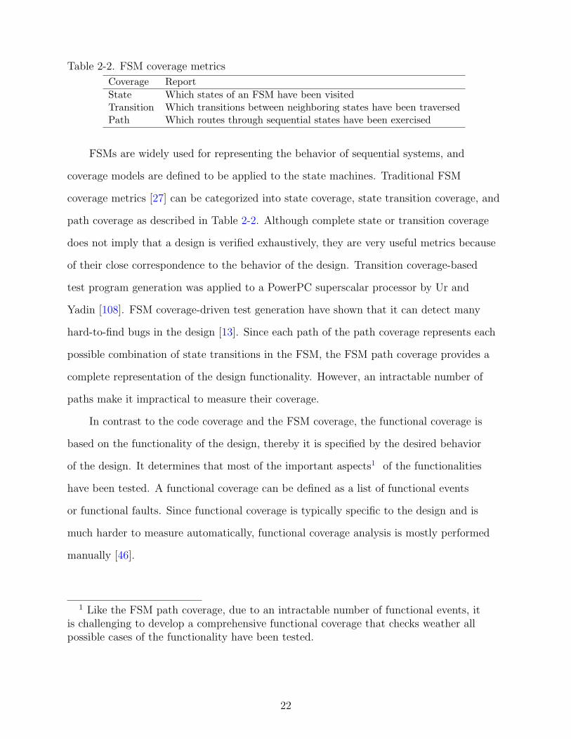
Table 2-2. FSM coverage metrics
Coverage ReportState Which states of an FSM have been visitedTransition Which transitions between neighboring states have been traversedPath Which routes through sequential states have been exercised
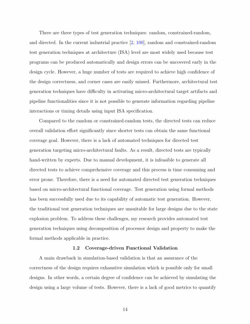
FSMs are widely used for representing the behavior of sequential systems, and
coverage models are defined to be applied to the state machines. Traditional FSM
coverage metrics [27] can be categorized into state coverage, state transition coverage, and
path coverage as described in Table 2-2. Although complete state or transition coverage
does not imply that a design is verified exhaustively, they are very useful metrics because
of their close correspondence to the behavior of the design. Transition coverage-based
test program generation was applied to a PowerPC superscalar processor by Ur and
Yadin [108]. FSM coverage-driven test generation have shown that it can detect many
hard-to-find bugs in the design [13]. Since each path of the path coverage represents each
possible combination of state transitions in the FSM, the FSM path coverage provides a
complete representation of the design functionality. However, an intractable number of
paths make it impractical to measure their coverage.
In contrast to the code coverage and the FSM coverage, the functional coverage is
based on the functionality of the design, thereby it is specified by the desired behavior
of the design. It determines that most of the important aspects1 of the functionalities
have been tested. A functional coverage can be defined as a list of functional events
or functional faults. Since functional coverage is typically specific to the design and is
much harder to measure automatically, functional coverage analysis is mostly performed
manually [46].
1 Like the FSM path coverage, due to an intractable number of functional events, itis challenging to develop a comprehensive functional coverage that checks weather allpossible cases of the functionality have been tested.
22

Azatchi et al. [11] have presented analysis techniques for a cross-product functional
coverage [51] by providing manual analysis techniques as well as fully automated coverage
analysis. To extract useful information out of the coverage data, they described coverage
queries that combine manual and automatic analysis and find holes that contain specific
coverage events. In the cross-product coverage, the list of coverage events consists of
all possible Cartesian products of the values for a given set of attributes. Based on the
cross-product coverage, Ziv [116] has proposed functional coverage measurement with
temporal properties-based assertions. Hole analysis for discovering large uncovered spaces
for cross-product functional coverage model was presented by Lachish et al. [74]. The
problem with the cross-product coverage is that the number of cross-product events is too
large to enable fast analysis. In addition, it is necessary to distinguish legal events since
not all attributes are independent thereby many of the cross-product events can never be
executed.
Piziali [92] described other types of functional coverage models as collections of
discrete events, trees, and hybrid models that combine trees and cross-product. Fournier
et al. [46] have proposed the validation suite for the PowerPC architecture based on a
set of combinational coverage models. Mishra and Dutt [85] have proposed a node/edge
coverage of the graph model of pipelined processors to generate tests. Recently, Harris
[53] has proposed a behavioral coverage metric which evaluates the validation of the
interactions between processes.
2.2 Graph-based Modeling of Pipelined Processors
The structure of a pipelined processor can be modeled as a graph G = (V, E). Nodes
V denotes two types of components in the processor: units (e.g., Fetch, Decode, etc) and
storages (e.g., register file or memory). Edges E consists of two types of edges: pipeline
edges and data transfer edges. A pipeline edge transfers an instruction (operation) from
a parent unit to a child unit. A data-transfer edge transfers data between units and
storages. This graph model is similar to the pipeline level block diagram available in a
23
MainMemory
Memory
RegFile
Fetch
FADD1
FADD2
FADD4
FADD3
WriteBack
MEM
MUL7
MUL2
MUL1IALU
Data
DIV
PC
Decode
Memory
StorageInstruction FlowData Transfer
Unit
Instruction
17
12
16
1
2
3 4
5
10
11
13
14
15
Figure 2-1. Graph model of the MIPS processor
typical architecture manual. This section presents graph models for a MIPS processor and
a PowerPC e500 processor.
2.2.1 Modeling of MIPS processor
For illustration, we use a simplified version of the multi-issue MIPS processor [54].
Figure 2-1 shows the graph model of the processor that can issue up to four operations
(an integer ALU operation, a floating-point addition operation, a multiply operation,
and a divide operation). In the figure, rectangular boxes denote units, dashed rectangles
are storages, bold edges are instruction-transfer (pipeline) edges, and dashed edges are
data-transfer edges. A path from a root node (e.g., Fetch) to a leaf node (e.g, WriteBack)
consisting of units and pipeline edges is called a pipeline path. For example, one of the
pipeline path is {Fetch, Decode, IALU, MEM, WriteBack}. A path from a unit to main
memory or register file consisting of storages and data-transfer edges is called a data-
transfer path. For example, {MEM, DataMemory, MainMemory} is a data-transfer path.
24
Fetch stage 1
Fetch stage 2
Decode stage
Issue stage
MU stage 1
MU stage 2
MU stage 3
MU stage 4
Completion stage
Write-back stage
LSU stage 1
LSU stage 2
LSU stage 3
SU1 SU2
DividePost-divide
Execute stage
� 7 pipeline stages� Superscalar� Dynamic scheduling
RS RS
IQ
GIQ
I-cache
RenameBuffers
CompletionQueue
RS RS
D-cache
Figure 2-2. Instruction flow of the PowerPC e500 processor
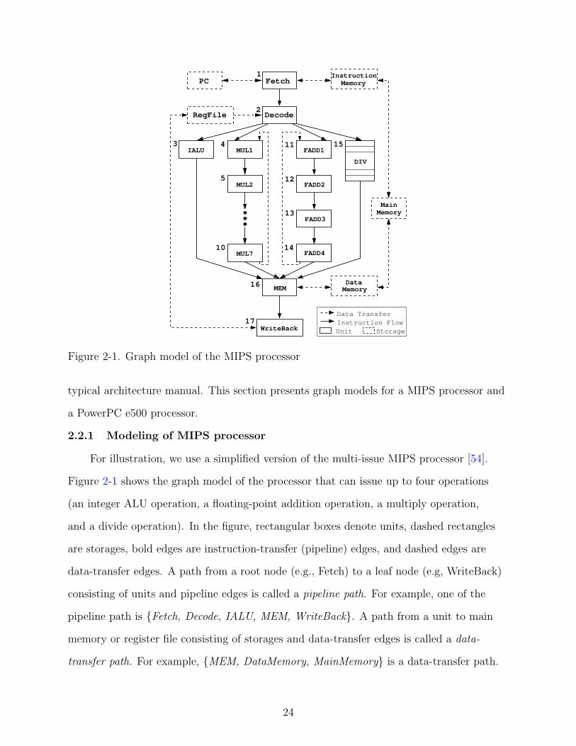
2.2.2 Modeling of PowerPC e500 processor
Figure 2-2 shows a functional graph model of the four-wide superscalar commercial
e500 processor based on the Power ArchitectureTM Technology2 [58] with seven pipeline
stages. We have developed a processor model based on the micro-architectural structure,
the instruction behavior, and the rules in each pipeline stage that determine when
instructions can move to the next stage. The micro-architectural features in the processor
model include pipelined and clock-accurate behaviors such as multiple issue for instruction
parallelism, out-of-order execution and in-order-completion for dynamic scheduling,
register renaming for removing false data dependency, reservation stations for avoiding
stalls at Fetch and Decode pipeline stages, and data forwarding for early resolution of
read-after-write (RAW) data dependency.
2 The Power Architecture and Power.org wordmarks and the Power and Power.org logosand related marks are trademarks and service marks licensed by Power.org
25

2.3 Pipeline Interaction Fault Model and Functional Coverage
Today’s test generation techniques and formal methods are very efficient to find
logical bugs in a single module. Hard-to-find bugs arise often from the inter-module
interactions among many pipeline stages and buffers of modern processor designs. In
this section, we primarily focus on such hard-to-verify interactions among modules in a
pipelined processor. If we consider the graph model of the pipelined processor described in
the previous section, the pipeline interactions imply the activities between the nodes in the
graph model.
We first define the possible pipeline interactions based on the number of nodes in the
graph model and the average number of activities in each node. For example, an IALU
node can have four activities: operation execution, stall, exception, and no operation
(NOP). In general, the number of activities for a node will be different based on what
activity we would like to test. For example, execution of ADD and SUB operations can be
treated as the same activity because they go through the same pipeline path. Separation
of them into different activities will refine the functional tests but increase the test
generation complexity. Furthermore, the number of activities varies for different nodes.
Considering a graph model with n nodes where each node can have on average r activities,
a total of r(1 − rn)/(1 − r) properties are required to verify all interactions. The basic
idea of the proof is that if we consider no interactions, there are (n × r) test programs
necessary. In the presence of one interaction we need (nC2 × r2) test programs for possible
combination of two nodes. nCi denotes the ways of choosing i nodes from n nodes. Based
on this model, the total number of interactions will be:
n∑i=1
nCi × ri (2–1)
Although the total number of interactions can be extremely large, in reality the
number of simultaneous interactions can be small and many other realistic assumptions
26

can reduce the number of properties to a manageable one. For example, we can consider
four functional activities in each node: operation execution, stall, exception, or NOP
(no-operation). A unit in “operation execution” carries out its functional operations
such as fetching an instruction, decoding opcode/operand, performing arithmetic/logic
computation, etc. The “Stall” in a unit can be caused by various reasons such as data
dependency, structural hazard, child node stall, etc. Exception in a node is an exceptional
state such as divide-by-zero or overflow. A pipeline interaction can be described as a
combination of nodes and their activities. We define two types of faults: node interaction
fault, and transition interaction fault.
• Node interaction fault model: An interaction is faulty if execution of multipleactivities at a given clock cycle does not correctly perform its interacted computation.
• Transition interaction fault model: A transition is faulty if a pipeline interaction ata given clock cycle does not correctly go through the pipeline interaction of the nextclock cycle.
The node interaction describes a snapshot behavior of a pipelined processor at a given
time, whereas the transition interaction captures the temporal behavior of the processor.
Comparing to FSM coverage, the node interaction faults and transition interaction faults
correspond to FSM state faults and FSM state transition faults. In the presence of a fault,
unexpected values will be written to the primary output such as data memory or register
file, or the test program will finish at incorrect clock cycle during simulation.
Using these pipeline interaction fault models, we define a functional coverage metric
with the consideration of the following cases:
• A node interaction fault is covered if the specified nodes are in their correct states atthe same clock cycle.
• A transition interaction fault is covered if two node interactions are exercisedconsecutively during clock transition.
The functional coverage (FC) is defined as follows:
FC =the number of faults detected by the test programs
total number of detectable faults in the fault model(2–2)
27

2.4 Chapter Summary
A coverage metric based on the functionality of pipelined processors is necessary for
the functional coverage-driven validation. This dissertation defines pipeline interaction
fault models. They are used to define a functional coverage as well as to facilitate
automated analysis of the functional coverage. It is important to note that the proposed
fault models are correspondent to FSM states and transitions respectively. In the following
chapters, the interaction faults are described as negated properties to produce directed test
programs.
28

CHAPTER 3TEST GENERATION USING DESIGN AND PROPERTY DECOMPOSITIONS
A significant bottleneck in processor validation is the lack of automated tools and
techniques for directed test generation. Model checking-based test generation has been
introduced as a promising approach for pipelined processor validation due to its capability
of automatic test generation. However, traditional approaches are unsuitable for large
designs due to the state explosion problem in model checking. We propose an efficient
test generation technique using both design and property decompositions to enable model
checking-based test generation for complex designs.
Processor modelProcessor model
Test generation
Test cases
PropertiesProperties
Propertydecomposition
Modeldecomposition
Architecturalspecification
Figure 3-1. Test generation methodology using design and property decompositions
Figure 3-1 shows our functional test program generation methodology. The processor
model can be generated from the architecture specification or can be developed by the
designers. The properties can be generated from the specification based on a functional
coverage such as graph coverage or pipeline interaction coverage. Additional properties can
be added based on interesting scenarios using combined pipeline stage rules and corner
cases. For efficient test generation, we decompose the properties as well as the processor
model. Model checker and SAT solver are used to generate partial counterexamples for
29
the partitioned modules and decomposed properties. These partial counterexamples are
integrated to construct the final test program.
The proposed methodology makes three important contributions: i) it develops a
procedure for decomposing a temporal logic property into multiple smaller properties,
ii) it presents an algorithm for merging the counterexamples generated by decomposed
properties, and iii) it develops an integrated framework to support both design and
property decompositions for efficient test generation of pipelined processors.
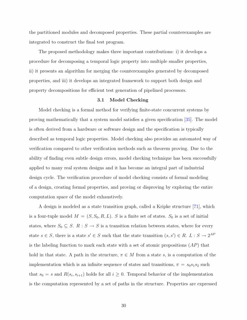
3.1 Model Checking
Model checking is a formal method for verifying finite-state concurrent systems by
proving mathematically that a system model satisfies a given specification [35]. The model
is often derived from a hardware or software design and the specification is typically
described as temporal logic properties. Model checking also provides an automated way of
verification compared to other verification methods such as theorem proving. Due to the
ability of finding even subtle design errors, model checking technique has been successfully
applied to many real system designs and it has become an integral part of industrial
design cycle. The verification procedure of model checking consists of formal modeling
of a design, creating formal properties, and proving or disproving by exploring the entire
computation space of the model exhaustively.
A design is modeled as a state transition graph, called a Kripke structure [71], which
is a four-tuple model M = (S, S0, R, L). S is a finite set of states. S0 is a set of initial
states, where S0 ⊆ S. R : S → S is a transition relation between states, where for every
state s ∈ S, there is a state s′ ∈ S such that the state transition (s, s′) ∈ R. L : S → 2AP
is the labeling function to mark each state with a set of atomic propositions (AP ) that
hold in that state. A path in the structure, π ∈ M from a state s, is a computation of the
implementation which is an infinite sequence of states and transitions, π = s0s1s2 such
that s0 = s and R(si, si+1) holds for all i ≥ 0. Temporal behavior of the implementation
is the computation represented by a set of paths in the structure. Properties are expressed
30

as propositional temporal logic that describes sequences of transitions on the computation
paths of expected design behavior. A property is composed of three things as follows:
• Atomic propositions: variables in the design.
• Boolean connectives: AND, OR, NOT, IMPLY, etc.
• Temporal operators, assuming p is a state or path formula:
1. Fp (Eventually): True if there exists a state on the path where p is true.
2. Gp (Always): True if p is true at all states on the path.
3. Xp (Next): True if p is true at the state immediately after the current state.
4. p1Up2 (Until): True if p2 is true in a state and p1 is true in all preceding states.
For example, the property G(req → F (ack)) describes that if req is asserted then the
design must eventually reach a state where ack is asserted.
Given a formal model M = (S, S0, R, L) of a design and a propositional temporal
logic property p, the model checking problem is to find a set of all states in S that satisfy
p, {s ∈ S|M, s| = p}. If all initial states are in the set, the design satisfies the property. If
the property does not hold for the design, a trace from the error state to an initial state
is given as a counterexample that helps designers debug the error. To achieve complete
confidence of correctness of the design, the specification1 should include all the properties
that the design should satisfy.
Due to the high complexity of realistic designs, the number of states of the design can
be very large and the explicit traversal of the state space becomes infeasible, known as
the state explosion problem. To alleviate this problem, symbolic model checking [22, 80]
represents the finite state machine of the design in the form of binary decision diagrams
1 The hardware design process is divided into several steps based on refinement levelof abstractions. The next lower level of the specification on a certain abstraction level iscalled implementation. If we partition the hardware design process into architecture-level,RTL (register transfer level), gate level, transistor level, and layout level, then RTL designis implementation of architecture design whereas RTL design is specification of the gatelevel design.
31

(BDDs) [19], a canonical form for boolean expression. More than 1020 states can be
handled by BDD-based model checkers. More recently, SAT solvers have been applied
to bounded model checking [15, 16]. The basic idea behind SAT-based bounded model
checking is to consider counterexamples of a particular length and produce a propositional
formula that is satisfiable if such a counterexample exists. This technique can not only
generate counterexamples much faster of minimal length but also handle larger number of
states of the design compared to traditional symbolic model checking.
Despite the success of symbolic model checking, the state explosion problem is still
challenging in applying to large designs of industrial strength. To reduce the number
of states of the design model, a lot of techniques have been proposed such as symmetry
reductions [31, 42, 82, 101], partial order reductions [5, 6, 12, 49, 91], and abstraction
techniques [9, 10, 32, 36, 39, 61, 76]. Among these techniques, combining model checking
with abstraction has been successfully applied to verify a pipeline ALU circuit with
more than 101300 reachable states [33]. The proposed test generation approaches in this
dissertation fit in the abstraction techniques in that the components of the original design
model that are irrelevant to a given property are removed through the decomposition of
design and property under consideration.
3.2 Test Generation using Model Checking
Test generation using model checking is one of the most promising directed test
generation approaches due to its capability of automatically producing a counterexample.
SpecificationSpecification
Model checker
Counterexample
(Test)
PropertiesProperties
Figure 3-2. Test generation using model checking
32

Figure 3-2 shows a basic test generation framework using model checking. In this scenario,
a processor model is described in a temporal specification language and a desired behavior
is expressed in the form of temporal logic property. A model checker exhaustively searches
all reachable states of the model to check if the property holds (verification) or not
(falsification), which is called unbounded model checking. If the model checker finds any
reachable state that does not satisfy the property, it produces a counterexample. This
falsification can be quite effectively exploited for test generation. Instead of a desired
property, its negated version is applied to the model checker to produce a counterexample.
The counterexample contains a sequence of instructions from an initial state to a state
where the negated version of the property fails.
Processor modelProcessor model
Modelchecker
Counterexample
(Test)
PropertiesProperties
Processor architecture(ADL specification)
Figure 3-3. Specification-driven test generation using model checking
Specification-driven test generation using model checking has shown promising
results [86]. It can generate test programs at early design stage without any low-level
implementation knowledge. Figure 3-3 shows a specification-driven test program
generation scenario. A designer starts by specifying the processor architecture in an
Architecture Description Language (ADL) that is used to capture both the structure and
the behavior of the processor. A processor model is generated from the ADL specification.
Various properties (desired behaviors) are generated from the high level microarchitectural
33

processor specification. A model checker accepts the properties and the model of the
processor to produce test programs that are used for validation of the processor design.
However, the time and memory required for test generation are prohibitively large.
Furthermore, this method cannot be used for test generation of complex pipelined
processors due to the state explosion problem. This dissertation presents an efficient
test generation technique to reduce both test generation time and memory requirement
for complex processors. The proposed test generation approach reduces the search space
of counterexamples by decomposing design specification and properties [67, 69] and
restricting the length of counterexamples [68, 87].
3.3 Related Work
Traditionally, validation of microprocessors has been performed by applying a
combination of random and directed test programs using simulation-based techniques.
There are many successful test generation frameworks in industry today. Genesys-Pro
[2], used for functional verification of IBM processors, combines architecture and testing
knowledge for efficient test generation. In Piparazzi [2], a model of micro-architectural
processor and the user’s specification are converted into a Constraint Satisfaction
Problem (CSP) and the dedicated CSP solver is used to construct an actual test program.
Many techniques have been proposed for directed test program generation based on
an instruction tree traversal [4], micro-architectural coverage [70, 108], and functional
coverage using Bayesian Networks [44]. Recently, Gluska [48] described the need for
coverage directed test generation in coverage-oriented verification of the Intel Merom
microprocessor.
Several formal model-based test generation techniques have been developed for
validation of pipelined processors. In FSM-based test generation, FSM coverage is
used to generate test programs based on reachable states and state transitions [24,
56, 59, 65]. Since complicated micro-architectural mechanisms in modern processor
designs include interactions among many pipeline stages and buffers, the FSM-based
34

approaches suffer from the state space explosion problem. To alleviate the state explosion,
Utamaphethai et al. [109] have presented an FSM model partitioning technique based
on micro-architectural pipeline storage buffers. Similarly, Shen and Abraham [99] have
proposed an RTL abstraction technique that creates an abstract FSM model while
preserving clock accurate behaviors. Wagner et al. [112] have presented a Markov model
driven random test generator with activity monitors that provides assistance in locating
hard-to-find corner case design bugs and performance problems.
Model checking [35] has been successfully used in processor verification for proving
properties. Ho et al. [55] extract controlled token nets from a logic design to perform
efficient model checking. Jacobi [60] used a methodology to verify out-of-order pipelines
by combining model checking for the verification of the pipeline control, and theorem
proving for the verification of the pipeline functionality. Compositional model checking is
used to verify a processor microarchitecture containing most of the features of a modern
microprocessor [63]. Parthasarathy et al. [90] have presented a safety property verification
framework using sequential SAT and bounded model checking. Model checking based
techniques are also used in the context of falsification by generating counterexamples.
Clarke et al. [34] have presented an efficient algorithm for generation of counterexamples
and witnesses in symbolic model checking. Bjesse et al. [17] have used counterexample
guided abstraction refinement to find complex bugs. Automatic test generation techniques
using model checking have been proposed in software [47] as well as in hardware validation
[83]. However, traditional model checking based techniques does not scale well due to
the state space explosion problem. To reduce the test generation time and memory
requirement, Mishra and Dutt [84, 85] have proposed a design decomposition technique at
the module level when the original property contains variables for only a single module.
However, their technique does not handle properties that have variables from multiple
modules. Such properties are common in test generation. Our framework allows such
35
input properties by decomposing the properties as well as the model of the pipelined
processor.
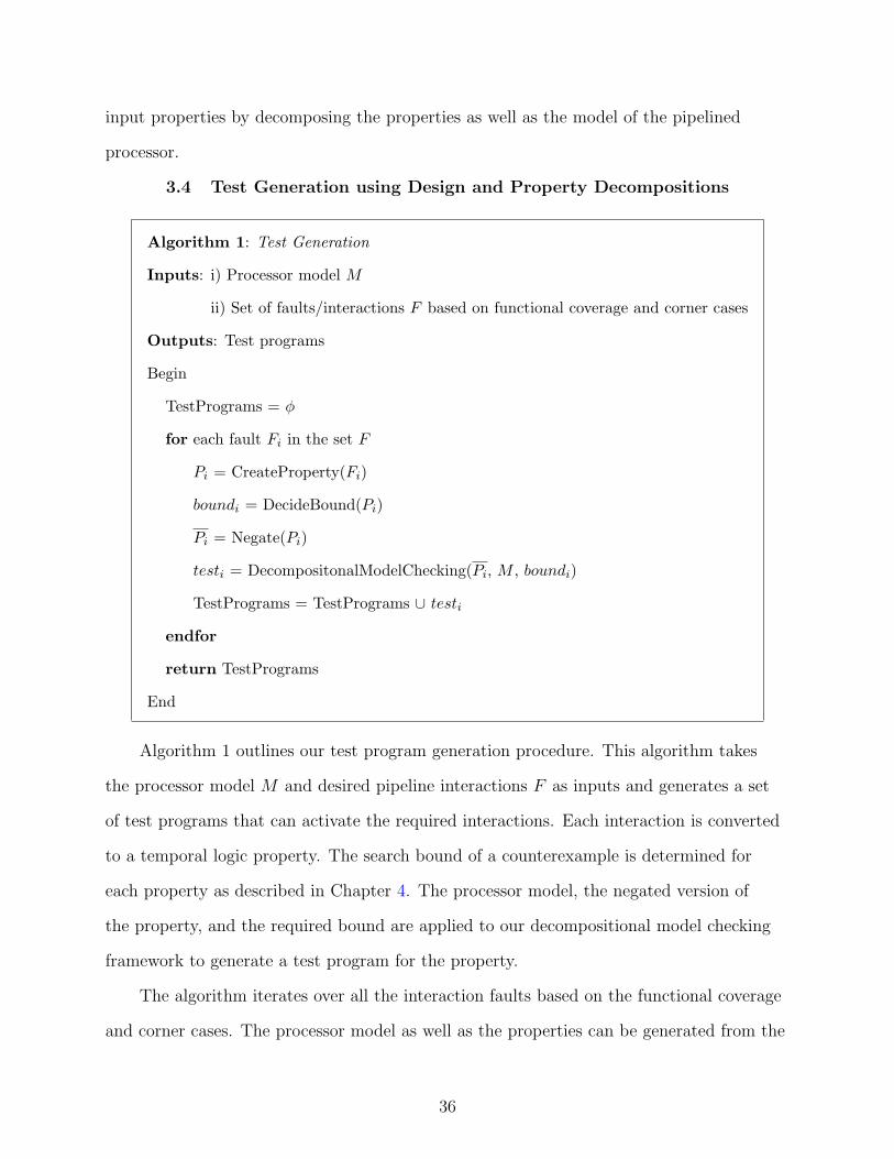
3.4 Test Generation using Design and Property Decompositions
Algorithm 1: Test Generation
Inputs: i) Processor model M
ii) Set of faults/interactions F based on functional coverage and corner cases
Outputs: Test programs
Begin
TestPrograms = φ
for each fault Fi in the set F
Pi = CreateProperty(Fi)
boundi = DecideBound(Pi)
Pi = Negate(Pi)
testi = DecompositonalModelChecking(Pi, M , boundi)
TestPrograms = TestPrograms ∪ testi
endfor
return TestPrograms
End
Algorithm 1 outlines our test program generation procedure. This algorithm takes
the processor model M and desired pipeline interactions F as inputs and generates a set
of test programs that can activate the required interactions. Each interaction is converted
to a temporal logic property. The search bound of a counterexample is determined for
each property as described in Chapter 4. The processor model, the negated version of
the property, and the required bound are applied to our decompositional model checking
framework to generate a test program for the property.
The algorithm iterates over all the interaction faults based on the functional coverage
and corner cases. The processor model as well as the properties can be generated from the
36
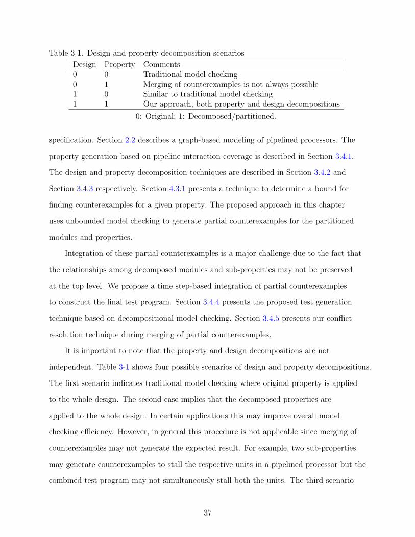
Table 3-1. Design and property decomposition scenarios
Design Property Comments0 0 Traditional model checking0 1 Merging of counterexamples is not always possible1 0 Similar to traditional model checking1 1 Our approach, both property and design decompositions
0: Original; 1: Decomposed/partitioned.
specification. Section 2.2 describes a graph-based modeling of pipelined processors. The
property generation based on pipeline interaction coverage is described in Section 3.4.1.
The design and property decomposition techniques are described in Section 3.4.2 and
Section 3.4.3 respectively. Section 4.3.1 presents a technique to determine a bound for
finding counterexamples for a given property. The proposed approach in this chapter
uses unbounded model checking to generate partial counterexamples for the partitioned
modules and properties.
Integration of these partial counterexamples is a major challenge due to the fact that
the relationships among decomposed modules and sub-properties may not be preserved
at the top level. We propose a time step-based integration of partial counterexamples
to construct the final test program. Section 3.4.4 presents the proposed test generation
technique based on decompositional model checking. Section 3.4.5 presents our conflict
resolution technique during merging of partial counterexamples.
It is important to note that the property and design decompositions are not
independent. Table 3-1 shows four possible scenarios of design and property decompositions.
The first scenario indicates traditional model checking where original property is applied
to the whole design. The second case implies that the decomposed properties are
applied to the whole design. In certain applications this may improve overall model
checking efficiency. However, in general this procedure is not applicable since merging of
counterexamples may not generate the expected result. For example, two sub-properties
may generate counterexamples to stall the respective units in a pipelined processor but the
combined test program may not simultaneously stall both the units. The third scenario
37

is meaningless since design decomposition is not useful if the original property is not
applicable to the partitioned design components. The last scenario depicts our approach
where both design and properties are partitioned.
3.4.1 Generation and Negation of Properties
The pipeline interaction properties described in Section 2.3 are expressed in linear
temporal logic (LTL) [35] where each property consists of temporal operators (G, F,
X, U) and Boolean connectives (∧, ∨, ¬, and →). We generate a property for each
pipeline interaction from the specification. Since pipeline interactions at a given cycle are
semantically explicit and our processor model is organized as structure-oriented modules,
pipeline interactions can be converted in the form of a property such as F(p1 ∧ p2 ∧. . .∧ pn) that combines activities pi over n modules using logical AND operator. The
atomic proposition pi is a functional activity at a node i such as operation execution,
stall, exception or NOP. The property is true when all the pi’s (i = 1 to n) hold at some
time step. Since we are interested in counterexample generation, we need to generate the
negation of the property first. The negation of the properties can be expressed as:
¬X(p) = X(¬p),¬G(p) = F (¬p)
¬F (p) = G(¬p),¬pUq = pR¬q (3–1)
For example, the negation of F(p1 ∧ p2 ∧ . . .∧ pn), interaction fault, can be described
as G(¬p1 ∨ ¬p2 ∨ . . .∨ ¬pn) whose counterexamples will satisfy the original property. In
the following section, we describe how to decompose these properties (already negated) for
efficient test generation using model checking.
3.4.2 Property Decomposition
Various combinations of temporal operators and Boolean connectives are possible
to express desired properties in temporal logic. If the properties are decomposable, the
partial counterexamples generated from the decomposed properties can be used for
generating a counterexample of the original property. However, not all properties are
38
decomposable, and in certain situations decompositions are not beneficial compared to
traditional model checking-based test generation. This section describes how to decompose
these properties (already negated) in respect to generation of a counterexample. We
assume that a set of counterexamples always exist for the original property since the
original property is the negated version of the desired property and the design is assumed
to be correct.
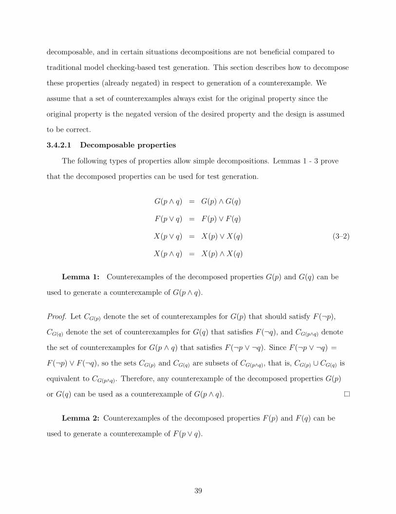
3.4.2.1 Decomposable properties
The following types of properties allow simple decompositions. Lemmas 1 - 3 prove
that the decomposed properties can be used for test generation.
G(p ∧ q) = G(p) ∧G(q)
F (p ∨ q) = F (p) ∨ F (q)
X(p ∨ q) = X(p) ∨X(q) (3–2)
X(p ∧ q) = X(p) ∧X(q)
Lemma 1: Counterexamples of the decomposed properties G(p) and G(q) can be
used to generate a counterexample of G(p ∧ q).
Proof. Let CG(p) denote the set of counterexamples for G(p) that should satisfy F (¬p),
CG(q) denote the set of counterexamples for G(q) that satisfies F (¬q), and CG(p∧q) denote
the set of counterexamples for G(p ∧ q) that satisfies F (¬p ∨ ¬q). Since F (¬p ∨ ¬q) =
F (¬p) ∨ F (¬q), so the sets CG(p) and CG(q) are subsets of CG(p∧q), that is, CG(p) ∪ CG(q) is
equivalent to CG(p∧q). Therefore, any counterexample of the decomposed properties G(p)
or G(q) can be used as a counterexample of G(p ∧ q).
Lemma 2: Counterexamples of the decomposed properties F (p) and F (q) can be
used to generate a counterexample of F (p ∨ q).
39

Proof. Since G(¬p ∧ ¬q) = G(¬p) ∧ G(¬q), so the set CF (p∨q) is equal to the intersection
of CF (p) and CF (q), that is, CF (p) ∩ CF (q) is equivalent to CF (p∨q). Therefore, a common
counterexample between F (p) and F (q) can be used as a counterexample of F (p ∨ q).
Lemma 3: Counterexamples of the decomposed properties X(p) and X(q) can be
used to generate a counterexample of X(p ∧ q) and X(p ∨ q).
Proof. Since X(¬p ∨ ¬q) = X(¬p) ∨ X(¬q), so the sets CX(p) and CX(q) are subsets of
CX(p∧q), that is, CX(p) ∪ CX(q) is equivalent to CX(p∧q). Therefore, any counterexample of
the decomposed properties X(p) or X(q) can be used as a counterexample of X(p ∧ q).
In addition, since X(¬p ∧ ¬q) = X(¬p) ∧ X(¬q), so the set CX(p∨q) is equal to the
intersection of CX(p) and CX(q), CX(p) ∩ CX(q) is equivalent to CX(p∨q). Therefore, a
common counterexample between X(p) and X(q) can be used as a counterexample of
X(p ∨ q).
3.4.2.2 Non-decomposable properties
It is important to note that the property decomposition is not possible in various
scenarios when the combination of decomposed properties is not logically equivalent to the
original property. For example, F (p∧q) 6= F (p)∧F (q), and G(p∨q) 6= G(p)∧G(q). However,
with respect to test generation, the counterexamples of the decomposed properties can be
used to generate a counterexample of the original property as described below.
The property F (p ∧ q) is true when both p and q hold at the same time step.
But F (p) ∧ F (q) is true even when p and q hold at different time steps. Therefore,
F (p ∧ q) 6= F (p) ∧ F (q). However, we can use F (p) and F (q) for test generation to activate
the property F (p ∧ q) based on Lemma 4.
Lemma 4: Counterexamples of the decomposed properties F (p) and F (q) can be
used to generate the counterexample of F (p ∧ q).
40

Proof. Since the relation between F (p ∧ q) and F (p) ∧ F (q) is F (p ∧ q) → F (p) ∧ F (q),
so CF (p∧q) ⊃ (CF (p) ∪ CF (q)). Therefore, any counterexample of the decomposed properties
F (p) or F (q) is a counterexample of F (p ∧ q).
The property G(p ∨ q) is true when either p or q holds at every time step. But
G(p) ∨ G(q) is true either when p holds at every time step, or when q holds at every
time step. Therefore, G(p ∨ q) 6= G(p) ∨ G(q). In this case, the counterexamples
of the decomposed properties G(p) and G(q) cannot directly be used to generate a
counterexample of G(p) ∨ G(q) since G(p) ∨ G(q) → G(p ∨ q), that is, (CG(p) ∩ CG(q)) ⊃CG(p∨q). In other words, not all common counterexamples of G(p) and G(q) can be
used as a counterexample of G(p ∨ q). Furthermore, it is hard to know whether the
common counterexamples of G(p) and G(q) belong to CG(p∨q). To address this problem,
this dissertation proposes a scheme of introducing the notion of clock that allows the
decomposed properties to produce a counterexample of G(p ∨ q) as described in Lemma 5.
Lemma 5: Counterexamples of G(p) and G(q) can be used to generate a counterexample
of G(p ∨ q) by introducing a specific time step.
Proof. The relation between G(p ∨ q) and G(p) ∨ G(q) with time step is G((clk 6=ts) ∨ (p ∨ q)) = G((clk 6= ts) ∨ p) ∨ G((clk 6= ts) ∨ q) because both sides are evaluated
true when (clk 6= ts), or when (clk = ts) and p = true or q = true. Therefore,
CG((clk 6=ts)∨(p∨q)) ≡ (CG((clk 6=ts)∨p) ∩ CG((clk 6=ts)∨q)).
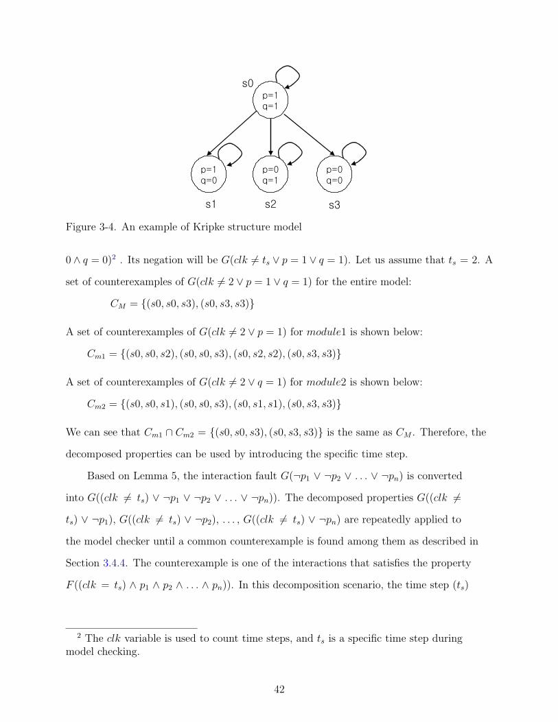
For example, Figure 3-4 describes a Kripke structure [35] with four states s0, s1, s2,
and s3, where s0 is the only initial state. The structure has three transitions: (s0, s1),
(s0, s2), (s0, s3), and self-loop in each state. There are two local variables p for module1
and q for module2 : p holds on states {s0, s1} and q holds on states {s0, s2}. Assuming
the original property is F (p = 0∧q = 0), a specific time step is introduced F (clk = ts∧p =
41
p=1
q=1
p=1
q=0
p=0
q=1
p=0
q=0
s0
s1 s2 s3
Figure 3-4. An example of Kripke structure model
0 ∧ q = 0)2 . Its negation will be G(clk 6= ts ∨ p = 1 ∨ q = 1). Let us assume that ts = 2. A
set of counterexamples of G(clk 6= 2 ∨ p = 1 ∨ q = 1) for the entire model:
CM = {(s0, s0, s3), (s0, s3, s3)}
A set of counterexamples of G(clk 6= 2 ∨ p = 1) for module1 is shown below:
Cm1 = {(s0, s0, s2), (s0, s0, s3), (s0, s2, s2), (s0, s3, s3)}
A set of counterexamples of G(clk 6= 2 ∨ q = 1) for module2 is shown below:
Cm2 = {(s0, s0, s1), (s0, s0, s3), (s0, s1, s1), (s0, s3, s3)}
We can see that Cm1 ∩ Cm2 = {(s0, s0, s3), (s0, s3, s3)} is the same as CM . Therefore, the
decomposed properties can be used by introducing the specific time step.
Based on Lemma 5, the interaction fault G(¬p1 ∨ ¬p2 ∨ . . . ∨ ¬pn) is converted
into G((clk 6= ts) ∨ ¬p1 ∨ ¬p2 ∨ . . . ∨ ¬pn)). The decomposed properties G((clk 6=ts) ∨ ¬p1), G((clk 6= ts) ∨ ¬p2), . . . , G((clk 6= ts) ∨ ¬pn) are repeatedly applied to
the model checker until a common counterexample is found among them as described in
Section 3.4.4. The counterexample is one of the interactions that satisfies the property
F ((clk = ts) ∧ p1 ∧ p2 ∧ . . . ∧ pn)). In this decomposition scenario, the time step (ts)
2 The clk variable is used to count time steps, and ts is a specific time step duringmodel checking.
42
should be decided to guarantee that a counterexample exist within the given bound (ts).
As described in the analysis of bounded model checking techniques [8], deciding bound
is a challenging problem since the depth of counterexamples is unknown in most cases.
Section 4.3.1 describes a way of deciding the bound (ts) that enables test generation using
SAT-based bounded model checking.
For certain properties such as pUq, F (p → F (q)), F (p → G(q)), G(p → G(q)), or
G(p → F (q)), decompositions are not beneficial compared to traditional model checking
because it is very difficult to decide a specific time step between their decomposed
properties. Although many property decompositions are not possible, it is important
to note that the scenarios described in this section are sufficient to generate the test
programs in the context of pipeline interactions. In addition to these interaction
properties, many micro-architectural properties have been created that are based on
real experiences of industrial designers for test generation of an e500 processor.
An important consideration during property decomposition is how to specify/handle
the different types of variables in the property. In general, the properties are described
as pairs of module names and variable names. An interaction fault property pi can be
either a local variable in a single module or a global variable over multiple modules. If pi
is a local variable, it is converted into (mi.pi) where mi is the corresponding module. If pi
is a global variable, pi is decomposed into sub-properties of corresponding modules. For
example, for the property G(¬p1 ∨ ¬p2), if p1 is an interface variable between m1 and m2,
then the property is converted as G(¬m1.p1 ∨ (¬m2.p1 ∨¬m2.p2)). Decomposition of global
variables is based on the decomposed modules of a processor model and their interfaces.
3.4.3 Design Decomposition
Decomposition of a design plays a central role in the generation of efficient test
programs. Ideally, the design should be decomposed into components such that there is
very little interaction among the partitioned components. For a pipelined processor the
natural partition is along the pipeline boundaries as described in Section 2.2. In other
43
words, the partitioned pipelined processor can be viewed as a graph where nodes consist of
units (e.g., fetch, decode etc.) or storages (e.g., memory or register file), and edges consist
of connectivity among them. Typically, instruction is transferred between units, and data
is transferred between units and storages. This graph model is similar to the pipeline level
block diagram available in a typical architecture manual.
It is important to note that the design decomposition is dependent on the property
decomposition. The pipelined processor can be simply partitioned into functional modules.
However, we need to change the partitioning policy based on the properties. Because some
properties are hard to be decomposed at the module level when they are spread across
multiple modules or in the complicated forms such as pUq, F (p → G(q)), G(p → F (q)),
and so on. For example, a property may not be decomposable based on a module level
partitioning but it may be decomposable based on a pipeline path level partitioning.
We consider three partitioning techniques: module-level, path-level and stage-level
partitioning. Module (or node) level partitioning gives the lowest level of granularity in
the graph model in Figure 2-1. The integer-ALU pipeline path {Fetch, Decode, IALU,
MEM, WriteBack} is treated as one of the path level partitions. Similarly, the multiplier
path, the floating-point adder path, and the divider path are the other examples of
path level partitioning for the MIPS processor in Figure 2-1. Stage-level partitioning is
determined by the distance from the root node (e.g., Fetch). In general, various forms of
design and property partitioning are possible and different graph clustering algorithms
can be used to find different design partitions for a given property decomposition.
Section 3.4.4 describes two design partitioning techniques using illustrative examples.
3.4.4 Test Generation using Decompositional Model Checking
Algorithm 2 presents our decompositional model checking procedure (invoked
from Algorithm 1) for design and property decompositions. It applies the decomposed
properties (sub-properties) to model checking with the corresponding design partition, and
compose the generated partial counterexamples to construct the final test program.
44

Algorithm 2: DecompositionalModelChecking
Inputs: i) Property Pi, ii) Design D, iii) Bound boundi
Outputs: Test program
Begin
TaskList = φ; NextList = φ; AllList = φ; PrimaryInputs = φ; clk = boundi
{P 1i , P 2
i , ..., Pmi } = DecomposeProperty(Pi); {M1,M2, ..., Mn} = DecomposeDesign(D)
for each design partition Mj
TaskList[j] = AllList[clk][j] = P ji /* P j
i is applicable to Mj */
endfor
while TaskList is not empty and clk > 0
outRk = RemoveEntry(TaskList[k])
P ki = MergeRequirements(outRk, AllList, clk)
P ki = Negate(P k
i )
Counterexample = ModelChecking(P ki , Mk, clk)
inpRk = input requirements for Mk from Counterexample
if inpRk are not primary inputs
for each applicable parent node Mr of Mk
outRr = Extract output requirements for Mr from inpRk
NextList[r] = NextList[r] ∪ outRr
AllList[clk][r] = AllList[clk][r] ∪ outRr
endfor
else PrimaryInputs = PrimaryInputs ∪ inpRk
endif
if TaskList is empty
clk = clk − 1; TaskList = NextList; NextList = φ
endif
endwhile
if clk = 0 and TaskList is not empty
Report(boundi is too small); testi = φ
endif
else testi = ExtractInstructions(PrimaryInputs)
return testi
End
45
This algorithm accepts a property Pi (already negated in Algorithm 1), a design D,
and search bound boundi as inputs and produces the required test program. The property
is decomposed based on the techniques described in Section 3.4.2. Similarly, the design
is decomposed based on the property decomposition and the techniques described in
Section 3.4.3. This algorithm uses three lists to maintain the decomposed properties:
TaskList for the present clock cycle clk, NextList for the next cycle i.e., clk − 1,
and AllList for all properties. Each entry in the TaskList and the NextList contain
a collection of sub-properties that are applicable to corresponding design partitions.
Therefore, each list can have up to n entries where n is the number of design partitions in
the processor model. The tasks in the TaskList need to be performed in the current time
step (clk). The tasks in the NextList will be performed in the next time step (clk − 1).
AllList contains all the entries of TaskList for each time step. This information is used to
resolve the conflict among sub-properties as described in Section 3.4.5. Initially these lists
are empty.
The proposed algorithm generates one test program for each property set DPi
that consists of one or more sub-properties based on their applicability to different
modules or partitions in the design as discussed in Section 3.4.1. The algorithm adds
the sub-properties in the TaskList and AllList based on the partitions to which these
properties are applicable. The algorithm iterates over all the sub-properties in the
TaskList. It removes an entry (say k-th location) from the TaskList which is the output
requirement outRk of k-th partition. In general, this entry can be a list of sub-properties
(due to simultaneous output requirements from multiple children nodes) that need to be
applied to partition Mk. These sub-properties are composed to create the intermediate
property P ki using MergeRequirements procedure described in Section 3.4.5. After
negation of P ki , the property P k
i is applied to the corresponding partition Mk using the
model checker to generate a counterexample. The generated counterexample is analyzed
to find the input requirements inpk for the partition Mk. If these are primary inputs
46
(inputs of the root node in the graph model), then they are stored in PrimaryInputs list.
Otherwise, for each parent node Mr to which inpk is applicable, the algorithm extracts
the output requirements for Mr. This output requirement is added to the r-th entry of
the NextList as well as to the AllList. Finally, if the tasks for the current time step
is completed (TaskList empty), NextList is copied to the TaskList and the time step
clk is reduced by one. This process continues until both the lists are empty. Using the
precise bound (boundi) for the original property Pi enables the clk to be zero and two lists
empty at the same time. If the boundi is larger than the counterexample of Pi, two lists
will empty before the clk becomes zero. These two cases imply that we have obtained the
primary input assignments for all the sub-properties. These assignments are converted
into a test program consisting of a sequence of instructions. However, if the time step clk
reaches zero even when sub-properties remain in the lists, then the boundi needs to be
assigned a larger value. This implies that all the counterexamples of Pi exist out of the
boundi.
For illustration, consider a simple property P1 to verify a multiple execution scenario
consisting of IALU (3rd module) and DIV (15th module) nodes in Figure 2-1 at clock
cycle 5. We assume the module level partitioning of the design for this example. The
property can be decomposed into two sub-properties P 31 (IALU not stalled in cycle 5)
and P 151 (DIV not stalled in cycle 5). This implies that TaskList will have two entries
before entering the while loop: TaskList[3] = P 31 and TaskList[15] = P 15
1 . At the
first iteration of the while loop P 31 will be applied to M3 (IALU) using model checker;
generated counter example will be analyzed to find the output requirement for the Decode
unit (2nd module in Figure 2-1) in clock cycle 4; and the requirement will be added
to NextList[2]. During second iteration of the while loop P 151 (TaskList[15]) will be
applied to M15 (DIV); generated counter example will be analyzed to find the output
requirement for the Decode unit in clock cycle 4; and the requirement will be added
to NextList[2]. At this point, the TaskList is empty and the NextList has only one
47
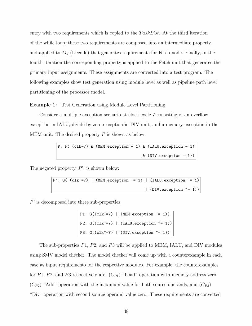
entry with two requirements which is copied to the TaskList. At the third iteration
of the while loop, these two requirements are composed into an intermediate property
and applied to M2 (Decode) that generates requirements for Fetch node. Finally, in the
fourth iteration the corresponding property is applied to the Fetch unit that generates the
primary input assignments. These assignments are converted into a test program. The
following examples show test generation using module level as well as pipeline path level
partitioning of the processor model.
Example 1: Test Generation using Module Level Partitioning
Consider a multiple exception scenario at clock cycle 7 consisting of an overflow
exception in IALU, divide by zero exception in DIV unit, and a memory exception in the
MEM unit. The desired property P is shown as below:
P: F( (clk=7) & (MEM.exception = 1) & (IALU.exception = 1)
& (DIV.exception = 1))
The negated property, P ’, is shown below:
P’: G( (clk~=7) | (MEM.exception ~= 1) | (IALU.exception ~= 1)
| (DIV.exception ~= 1))
P ’ is decomposed into three sub-properties:
P1: G((clk~=7) | (MEM.exception ~= 1))
P2: G((clk~=7) | (IALU.exception ~= 1))
P3: G((clk~=7) | (DIV.exception ~= 1))
The sub-properties P1, P2, and P3 will be applied to MEM, IALU, and DIV modules
using SMV model checker. The model checker will come up with a counterexample in each
case as input requirements for the respective modules. For example, the counterexamples
for P1, P2, and P3 respectively are: (CP1) “Load” operation with memory address zero,
(CP2) “Add” operation with the maximum value for both source operands, and (CP3)
“Div” operation with second source operand value zero. These requirements are converted
48

into properties and applied to the respective parent modules. In this case, P1’ (from CP1)
is applied to IALU, and P23’ (combine CP2 and CP3)3 is applied to the Decode unit in
the next step. In each case, clock cycle value is reduced by one as shown below:
P1’: G((clk~=6) | (aluOp.opcode ~= LD) | (aluOp.src1Val ~= 0))
P23’: G((clk~=6) | (decOp[0].opcode ~= ADD) | (decOp[0].src1Val ~= 2) |
(decOp[0].src2Val ~= 2) | (decOp[3].opcode ~= DIV) |
(decOp[3].src2Val ~= 0))
The outcome of the property P1’ will be applied to Decode unit (generates P1” say)
whereas the outcome of the P23’ will be applied to fetch unit (generate primary inputs
PIi) in time step 5. In time step 4, P1” will be applied to Fetch unit that generates the
primary inputs PIj. The primary inputs PIi and PIj are combined based on their time
step (clock cycle) to generate the final test program as shown below:
Fetch Instructions ([0] for ALU... [3] for DIV) \\
Cycle [0] [1] [2] [3] //R0 is 0
1 ADDI R2 R0 #2 NOP NOP NOP //R2 = 2
2 NOP NOP NOP NOP
3 NOP NOP NOP NOP
4 LD R1 0(R0) NOP NOP NOP
5 ADD R3 R2 R2 NOP NOP DIV R3 R0 R0
Example 2: Test Generation using Path-level Partitioning
The example shown above assumes a module-level partitioning of the processor
model. However, it is not always possible to decompose a property based on module
level partitioning. For example, if we are trying to determine whether two feedback
3 Note that when multiple children create requirements for the parent (e.g, P23’),conflicts can occur. In such cases, alternative assignments need to be evaluated for theconflicting variable as described in Section 3.4.5.
49

(data-forwarding) paths shown in Figure 2-1 are activated at the same time, it is not
possible to decompose this property at module level because the “implication” relation
between feedOut and feedIn (in the following property) will be lost.
To enable property decomposition in the this example, we need to partition the design
differently. The floating-point adder path (FADD1 to FADD4) should be treated as a
design partition Fpath. Similarly, the multiplier path (MUL1 to MUL7) should be treated
as another partition Mpath. This new partitioning is applied for test generation. First, P1
and P2 can be applied on Fpath and Mpath respectively to generate counterexamples C1
and C2. Next, C1 and C2 are combined and the corresponding property is applied to the
Decode unit to generate the counterexample C3. Next, the property corresponding to C3
is applied to the Fetch unit that generates the primary input requirements. Finally, these
primary input requirements are converted into the required test program. The property
decomposition procedure is shown below.
/* Original Property */
P: F((clk=9) & (FADD4.feedOut -> X(FADD1.feedIn))
& (MUL7.feedOut -> X(MUL1.feedIn)))
/* Converted Property */
P: F(((clk=9 & FADD4.feedOut) & (clk=10 & FADD1.feedIn))
& ((clk=9 & MUL7.feedOut) & (clk=10 & MUL1.feedIn)))
/* Property after Negation*/
P’: G(((clk~=9 | ~FADD4.feedOut) | (clk~=10 | ~FADD1.feedIn))
| ((clk~=9 | ~MUL7.feedOut) | (clk~=10 | ~MUL1.feedIn)))
/* Properties after Decomposition*/
P1: G((clk~=9 | ~FADD4.feedOut) | (clk~=10 | ~FADD1.feedIn))
P2: G((clk~=9 | ~MUL7.feedOut) | (clk~=10 | ~MUL1.feedIn))
50

3.4.5 Merging Partial Counterexamples
The output requirement (outRk in Algorithm 2) generated from a single child node
can be directly used for the corresponding module (Mk) simply by negating the output
requirement. In the case of multiple children, the input requirements generated from
children nodes need to be merged appropriately into the output property for the parent
node. However, this is non trivial since the input requirements can conflict each other
due to the fact that the model checker assigns arbitrary values to the variables that do
not have influence on falsification of the children nodes. For example, in Figure 2-2, four
reservation station (RS) modules share the parent module Issue. Counterexamples (input
requirements of each RS) generated from four RSs at the time step ts + 1 should be
combined for creating the output property of Issue module at clk = ts. However, they can
require different output values for the same variable of the module Issue.
In case of output requirement conflict, the algorithm adjusts input requirements of the
children nodes by excluding the current input requirement, called false requirement. For
example, assume that output variables of the parent are p and q, the input requirement of
one child is (p = 1 ∧ q = 0) that is generated by G((clk 6= (ts + 1)) ∨ ¬(m1.p = 1)) at
module1, and the input requirement of the other child is (p = 0 ∧ q = 1) that is generated
by G((clk 6= (ts + 1)) ∨ ¬(m2.q = 1)) at module2. Obviously, there is no way to assign
output p and q to satisfy these two conflicting inputs. We refine the sub-properties of
children nodes to resolve the conflict requirements by excluding the false requirement. The
desired sub-properties stored in AllList[ts + 1] for children nodes are modified by adding
the negated version of the conflict requirement as shown below:
F ((clk = (ts + 1)) ∧ (m1.p = 1) ∧ ¬(m1.p = 1 ∧m1.q = 0))
F ((clk = (ts + 1)) ∧ (m2.q = 1) ∧ ¬(m2.p = 0 ∧m2.q = 1))
To generate the input requirements of the module1, the above properties are negated as
shown below:
51
G((clk 6= (ts + 1)) ∨ ¬(m1.p = 1) ∨ (m1.p = 1 ∧m1.q = 0))
G((clk 6= (ts + 1)) ∨ ¬(m2.q = 1) ∨ (m2.p = 0 ∧m2.q = 1))
These sub-properties does not allow the counterexample (p = 1 ∧ q = 0) any more. The
generated counterexample will be (p = 1 ∧ q = 1) as the input requirements of module1
and module2. As a result, we can merge them into the output requirement of the parent
node as (p = 1 ∧ q = 1) at clk = ts. If there is an interface variable r between the
parent and its child module2, it does not cause the output requirement conflict of the
parent node since the input requirement of module1 does not care about the variable r. If
there is another child node module3 that has the interface variables p and r, we need to
adjust three input requirements of module1, module2, and module3 to resolve any conflict
among them. It is possible that there is no common variable assignments for shared input
variables among children nodes since their output requirements may be generated from
false input requirements from the subsequent stages (grandchildren nodes). In this case,
we need to refine the sub-properties of grandchildren nodes stored in AllList[ts + 2]. The
procedure of sub-property refinement continues until the conflict is resolved or clk is equal
to boundi which is upper bound to search for a test program.
3.5 Experiments
The proposed test generation methodology is applied on a multi-issue MIPS
architecture [54] and a superscalar commercial e500 processor [58]. Various test generation
experiments were performed for validating the pipeline interactions by varying different
design partitions and property decompositions. This section presents experimental results
in terms of time and memory requirement in test generation.
3.5.1 Test Generation using Module Level Decomposition
The test generation technique using UMC and module level decomposition is applied
on a multi-issue MIPS architecture as shown in Figure 2-1. SMV [79] model checker has
been used to perform all the experiments. Few simplifications was needed to the MIPS
processor to compare with two other approaches: i) naive approach where the original
52
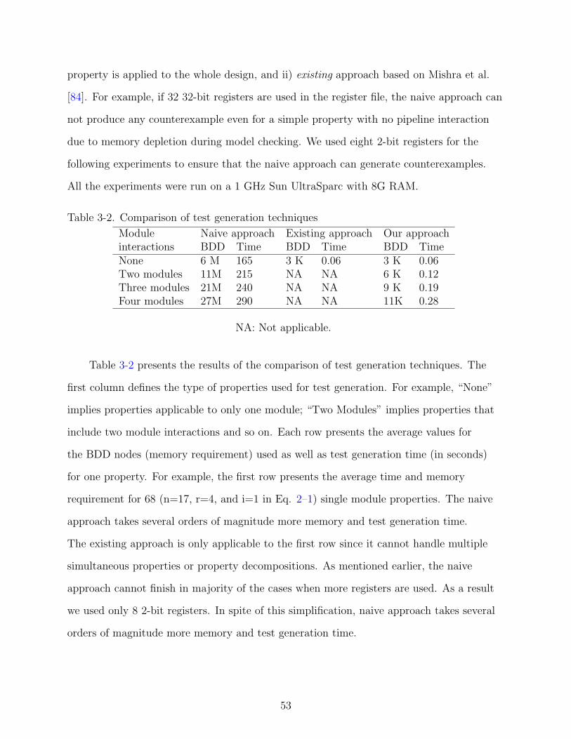
property is applied to the whole design, and ii) existing approach based on Mishra et al.
[84]. For example, if 32 32-bit registers are used in the register file, the naive approach can
not produce any counterexample even for a simple property with no pipeline interaction
due to memory depletion during model checking. We used eight 2-bit registers for the
following experiments to ensure that the naive approach can generate counterexamples.
All the experiments were run on a 1 GHz Sun UltraSparc with 8G RAM.
Table 3-2. Comparison of test generation techniques
Module Naive approach Existing approach Our approachinteractions BDD Time BDD Time BDD TimeNone 6 M 165 3 K 0.06 3 K 0.06Two modules 11M 215 NA NA 6 K 0.12Three modules 21M 240 NA NA 9 K 0.19Four modules 27M 290 NA NA 11K 0.28
NA: Not applicable.
Table 3-2 presents the results of the comparison of test generation techniques. The
first column defines the type of properties used for test generation. For example, “None”
implies properties applicable to only one module; “Two Modules” implies properties that
include two module interactions and so on. Each row presents the average values for
the BDD nodes (memory requirement) used as well as test generation time (in seconds)
for one property. For example, the first row presents the average time and memory
requirement for 68 (n=17, r=4, and i=1 in Eq. 2–1) single module properties. The naive
approach takes several orders of magnitude more memory and test generation time.
The existing approach is only applicable to the first row since it cannot handle multiple
simultaneous properties or property decompositions. As mentioned earlier, the naive
approach cannot finish in majority of the cases when more registers are used. As a result
we used only 8 2-bit registers. In spite of this simplification, naive approach takes several
orders of magnitude more memory and test generation time.
53

3.5.2 Test Generation for e500 Processor
The proposed decompositional model checking technique was also applied on a
superscalar PowerPC e500 processor.4 Our processor model includes micro-architectural
structure and clock accurate behaviors of the processor. We represented one clock cycle
as two time steps (low and high at each cycle) so that the processor model accommodates
the behaviors of read and write at the same cycle in the first-in-first-out (FIFO) queues
and reservation stations. We performed various test generation experiments for validating
the pipeline interactions and corner cases. In this section, we present a subset of the
test sequences generated by our test generation framework. Next, we describe how the
generated test programs are used in processor validation framework.
3.5.2.1 Results
Table 3-3 shows a subset of the directed test cases, their corresponding length in
terms of number of instructions, and test generation time. For example, the test program
for case 11 validates the feature of Completion Queue (CQ) by piling data up and down
in the first-in-first-out (FIFO) queue. Test programs for case 3 through 6 exercise operand
read from four different resources as shown in Figure 3-5, which can be generated at
micro-architecture level but very difficult at ISA level. In terms of efficiency, only several
seconds were spent on test generation except for the case 11 where test generation took
few minutes. The test cases 13-18 shows various interaction scenarios. For example, test
case 13 only activates one node whereas test case 15 considers three node interactions at
the same clock cycle.
3.5.2.2 Micro-architectural validation using test programs
Micro-architectural design errors such as performance bugs are hard to be exposed by
architectural test generation. Furthermore, they may not be detected by ISA functional
4 The e500 processor specification and RTL design were provided by FreescaleSemiconductor Inc.
54

Table 3-3. Various test cases generated by our framework
Test cases Test length Time1 Instruction dual issue 15 302 Renaming src1 operand 12 253 Read operand from forwarding path (RAW) 9 204 Reservation station reads operand from forwarding path 7 155 Read operand from renaming reg. (RAW) 10 206 Read operand from GPR (RAW) 11 257 Renaming for WAW (no stall) 8 208 Stall at Decode stage due to IQ full 14 359 Stall at Decode stage due to CQ full, then released queue 34 61
full at the next clock cycle10 CQ full, then full again 35 7011 CQ full, then empty, and then full again 95 29012 Retire only one instruction in Completion 12 2813 “lwz” instruction at LSU stage3 7 1514 “add” at Fetch 2 and “mulhw” at MU stage2 simultaneously 6 1815 “addi” at Completion, “mulhw” at MU stage1, & “lwz” at 12 25
LSU stage1 at the same clock16 “mulhw” at Completion, “add” & “addi” waits in 12 40
completion queue, & “lzw” at LSU stage317 “lwz” and “add” at Completion, “mulhw” at MU stage3, 14 35
“addi” at CQ, “lwz” at LSU stage118 “mulhw” & “add” retire, “mulhw” at MU stage4, 15 45
“addi” at CQ, & “lwz” at LSU-stage2
Issue Execute Complete Write-Back
ReservationStation
3 5 6
4 Instruction flow
Forwarding data
Figure 3-5. Four different data forwarding mechanisms
55

Micro-architecturaltest generation
RTPG
RTLsimulator
Functionalsimulator
CompareCheck if the faultis activated
Assembly sequence
Initializationinformation
Testbench
Functionaloutput
Instructionflow
Performance validation Functional validation
Figure 3-6. Micro-architectural validation flow
simulation. For example, test generation for uncovering incorrect stalls in pipeline stages
require timing information of instruction flow and those bugs are only visible during the
clock-accurate simulation. Therefore, micro-architectural validation plays an important
role in ensuring the correctness of performance as well as functionality of the processor
designs.
We have performed micro-architectural validation by using the existing methodology
in an industrial settings that includes an internal random test pattern generator (RTPG)
tool. Figure 3-6 shows the validation flow. We converted the assembly test sequences
generated by our method into the input format of the RTPG tool that produces
testbenches for RTL simulation. The simulator shows how instructions go through
the pipeline stages on a cycle-by-cycle basis as well as whether the stored results in
register files and memory are correct or not. Capturing when and which instructions
move from one stage to the next ensures that the generated tests exercise the target
micro-architectural artifacts. We compared the validation effort for activating these
micro-architectural features using the existing validation methodology in an industrial
setting and our approach. On an average each of our test case took less than 100 clock
56

cycles whereas the existing random/pseudo-random tests took approximately 100,000 clock
cycles to activate the target fault.
3.6 Chapter Summary
Functional verification is widely acknowledged as a major bottleneck in microprocessor
design methodology. Compared to the random or constrained-random tests, the directed
tests can reduce overall validation effort since shorter tests can obtain the same coverage
goal. However, there is a lack of automated techniques for directed test generation.
This chapter presented an efficient directed test generation technique for validation
of performance as well as functionality of the modern microprocessors. Our methodology
is based on decompositional model checking where the processor model as well as the
properties are decomposed and the model checking is applied on smaller partitions of the
design using decomposed properties. We introduced the notion of time steps to enable
decomposition of the properties into smaller ones based on their clock cycles. We have
developed an efficient algorithm to merge the partial counterexamples generated by the
decomposed properties to create the final test program corresponding to the original
property. Our experimental results using MIPS and PowerPC e500 processor architectures
demonstrate the efficiency of our method by generating complicated micro-architectural
tests. Since the proposed technique is generic, its framework can be used for validation of
other industrial-strength processors. Furthermore, this work can be seamlessly integrated
in the current RTPG validation methodology without modification of the existing
validation flow.
57

CHAPTER 4TEST GENERATION USING SAT-BASED BOUNDED MODEL CHECKING
Efficient test generation is crucial for the simulation-based validation since it
determines the quality of test suites as well as the performance of validation. This chapter
presents an efficient test generation methodology for functional validation of processor
designs using SAT-based bounded model checking (BMC).
As a complementary technique of unbounded model checking (UMC) in Chapter 3,
SAT-based bounded model checking (BMC) has given promising results in the verification
domain. The basic idea is to restrict the search space that is reachable from initial
states within a fixed number (k) of transitions, called the bound. After unwinding the
model of design k times, the BMC problem is converted into a propositional satisfiability
(SAT) problem. A SAT solver is used to find a satisfiable assignment of variables that is
converted into a counterexample. If the bound is known in advance, SAT-based BMC is
typically more effective for falsification than UMC because the search for counterexamples
is faster and the SAT capacity reaches beyond the BDD capacity [15]. However, finding
the bound is a challenging problem since the depth of counterexamples is unknown in
general.
Choosing an incorrect bound increases test generation time and memory requirement.
In the worst case, test generation may not be possible. For example, we can increase
the bound iteratively starting from a small bound until a counterexample is found. This
approach is advantageous for shallow counterexamples, but disadvantageous for deep
counterexamples due to accumulation of iterative running time. Another example is to
choose a large bound such that all counterexamples are found. This approach loses the
benefits of BMC due to search in a large number of irrelevant states when the bound is
too big. Therefore, the performance of test generation closely depends on the schemes of
deciding the bound. We propose a method to find the bound for each property instead of
using the maximum bound for all properties.
58

Processor architecture(Specification)
Processormodel
Properties
SAT-basedBMC
Decidebound
Negateproperty
Test programs
Faultmodel
Decompose(if necessary)
Decompose(if necessary)
Figure 4-1. Test program generation using SAT-based bounded model checking
Figure 4-1 shows our test generation methodology. Processor model and properties
are generated from the architecture specification. We use the pipeline interaction fault
model to define functional coverage. Temporal logic properties are created from pipeline
interaction faults. We determine the bound for each property to reduce test generation
time and memory requirement compared to using the maximum bound for all properties.
The processor model, negated properties, and the bound are applied to SAT-based BMC
to generate a test program. Based on the coverage report, more properties can be added, if
necessary. We use design and property decompositions to further improve the performance
of test generation. Our technique makes two important contributions: i) it develops a
procedure to determine the bound for each property, and ii) it presents a scheme for design
and property decompositions in the context of SAT-based BMC.
4.1 SAT-based Bounded Model Checking
Boolean satisfiability (SAT) problem is to determine whether there exists a variable
assignment such that a propositional formula evaluates to true. If there exists such
an assignment, the formula is called satisfiable. Otherwise, the formula is said to be
59

unsatisfiable. For example, the formula (a|¬b) ∧ (¬b|c) ∧ (¬c|¬a) is satisfiable when a = 1,
b = 0, and c = 0. SAT solver is a tool to check satisfiability of a given Boolean formula
represented in Conjunctive Normal Form (CNF)1 .
Bounded Model Checking (BMC) is a restricted form of model checking. Instead
of exhaustively searching a counterexample, BMC searches for a counterexample of a
particular length k, called bound or maximum length of counterexamples. The assumption
is that the property can be falsified (a counterexample exists) within k time steps.
In SAT-based BMC, the BMC problem is encoded into the satisfiability problem
and a SAT solver is used as a verification engine instead of a model checker. To perform
verification, SAT-based BMC includes the following steps:
1. Unfold design and property up to the bound k.
2. Encode the bounded design and property into a CNF formula.
3. Apply the CNF formula to a SAT solver.
4. If satisfiable, then the property does not hold for the design and the satisfiableassignment of variables is converted to a counterexample.
5. If unsatisfiable and k ≥ d (d: diameter2 ), then the property holds for the design, elseif unsatisfiable and k < d, then the property does not hold.
The CNF formula is satisfiable if and only if a violated state is reachable within the
bound k. The resulting satisfiable assignment of variables is translated into an error trace
from a valid initial state to the violated state. If the bound k is equal to or larger than
the diameter and the CNF formula is unsatisfiable, then the design satisfies the property
1 CNF is a conjunction of clauses, each clause is a disjunction of literals, and a literalis a Boolean variable or its negation. For example, the formula (a|¬b) ∧ (¬b|c) ∧ (¬c|¬a)conforms the CNF.
2 Diameter is the reachable longest time step in the state space of a given finite statesystem. By definition, any state that can be reached can be reached within the diameter.[81]
60

because there is no counterexample in the state space. However, if the bound k is smaller
than the diameter and the CNF formula is unsatisfiable, then SAT-based BMC cannot
prove or disprove the correctness of design since states beyond the bound k still remain
unchecked.
4.2 Related Work
Biere et al. [16] introduced bounded model checking (BMC) combined with
satisfiability solving. The recent developments in SAT-based BMC techniques have
been presented in [15, 30, 93]. BMC is an incomplete method that cannot guarantee a
true or false determination when a counterexample does not exist within a given bound.
However, once the bound of a counterexample is known, large designs can be falsified very
fast since SAT solvers [50, 78, 88, 114] do not require exponential space, and searching
counterexample in an arbitrary order consumes much less memory than breadth first
search in model checking.
The performance of bounded and unbounded algorithms was analyzed on a set of
industrial benchmarks in [7, 8]. The capacity increase of BMC techniques has become
attractive for industrial use. An Intel study [37] showed that BMC has better capacity and
productivity over unbounded model checking for real designs taken from the Pentium-4
processor. Recently, Gurumurthy et al. [52] have used BMC as test program generator for
mapping pre-computed module-level test sequences to processor instructions.
SAT-based BMC is one of the most promising test generation engines due to its
capacity and performance. However, finding the bound is a challenging problem. We
propose a method to determine the bound for each test generation scenario, thereby
making SAT-based BMC feasible in practice.
4.3 Test Generation using SAT-based Bounded Model Checking
During test generation, the processor model is described in a temporal specification
language such as SMV [79] or NuSMV [29]. We create negated properties and their
bounds. A SAT-based BMC unfolds the processor model along with a negated property
61

up to the bound and converts it into a conjunctive normal form (CNF) formula. A SAT
solver accepts the CNF formula as input and finds a satisfiable assignment of variables.
The satisfiable assignment is converted into a counterexample. To create a test program,
we extract a sequence of instructions from an initial state to a state where the negated
property fails.
Algorithm 2: Test Generation using SAT-based BMC
Inputs: i) Processor model M
ii) Set of faults S from interaction fault model
Outputs: Test programs to excite the pipeline interactions
Begin
TestPrograms = φ
for each fault Si in the set S
Pi = CreateProperty(Si)
Pi = Negate(Pi)
ki = DecideBound(Pi)
testi = DoSATbasedBMC(M , Pi, ki)
TestPrograms = TestPrograms ∪ testi
endfor
return TestPrograms
End
Algorithm 2 describes our test generation procedure. This algorithm takes processor
model M and interaction faults S as inputs and generates test programs. For each fault
Si, the algorithm produces one test program. Fault Si is composed of a set of node
activities and their relations. The algorithm iterates over all the interaction faults in the
fault model. Each fault Si is converted to a temporal logic property Pi. The procedure
for creating and negating the property is described in Section 3.4.1. Bound ki for each
property is decided as discussed in Section 4.3.1. SAT-based BMC takes processor model
62

M , negated properties Pi, and bound ki as inputs and generates a counterexample. A test
program is extracted by analyzing the counterexample.
So far, we assumed that the whole design model is applied to SAT-based BMC.
This approach is effective when the design is of moderate size and the bound is shallow.
However, for the test generation scenarios consisting of large designs and deep counterexamples,
SAT-based BMC may not be able to generate tests in a reasonable amount of time due
to large search space. In other words, the complexity problem still remains in SAT-based
BMC. In such cases, decompositions of property as well as design will reduce the test
generation complexity.
4.3.1 Determination of Bound
The bound for all interactions should be large enough to generate at least one
counterexample for the interaction whose state is farthest from the initial state. This
interaction can be reached by the longest pipeline path and data transfer path in the
graph model of pipelined processors. The longest path represents the largest number of
clock cycles for the first instruction to stay in the pipelined processor. Once an instruction
finishes its execution at the leaf node (e.g., WriteBack), the instruction does not affect the
execution flow of the following instructions any more. For example, in the graph model
of the MIPS processor in Figure 2-1, the maximum bound is determined by the length of
{FE→ DE→ IALU→ MEM→ Cache→ MM → Cache→ MEM→ WB} if cache miss takes
more time than any other pipeline paths. However, this bound is over-conservative in most
test scenarios because a lot of interactions do not include this longest path. Therefore,
using bound for each interaction is more efficient for test generation in terms of time and
memory requirement.
Bound for each interaction is determined by the longest temporal distance from
the root node to the nodes under consideration. For example, bound for the property
“IALU, FADD2, and FADD3 in operation execution at the same time” will be 5 because
FADD3 has the longest temporal distance from Fetch stage. If a property includes stall or
63

exception activity, the temporal distance between the root node and the leaf node (WB) is
added to consider the causal node of the stall or exception. After deciding counterexample
bound, either traditional model checking or SAT-based BMC can be used for generating
counterexamples by taking processor model, negated properties, and bound as inputs.
4.3.2 Design and Property Decompositions
Design and property decompositions can be used to further improve the test
generation performance. In this section, we consider only three partitioning techniques:
module-level partitioning, vertical (path-level) partitioning, and horizontal (stage-level)
partitioning. Depending on the properties, other forms of decompositions may be useful.
For example, module (or node) level partitioning provides the lowest level of granularity
in the graph model described in Section 2.2. However, SAT-based BMC at the module
level may not be beneficial anymore because UMC can handle small designs efficiently.
Experimental results in Section 4.4.3 show that UMC might be better for small designs.
In addition, module level decomposition is not always possible since local properties
are not preserved at the global level in general. However, the properties that are not
decomposable at module level may be decomposable by the horizontal and vertical
partitioning techniques.
4.4 A Case Study
We performed various test generation experiments to validate the pipeline interactions
by varying interactions of functional units and decompositions of design and properties.
We excluded illegal interactions based on the fact that their negated properties could
not generate any counterexample. In this section, we present our experimental setup
followed by test generation examples using horizontal and vertical decompositions. Next,
we compare our test generation technique with UMC-based test generation method as well
as BMC using the maximum bound.
64

4.4.1 Experimental Setup
We applied our methodology on a simplified MIPS architecture [12], as shown in
Figure 2-1. We chose the MIPS processor since it has been well studied in academia
and there are HDL implementations available for the processor that can be used for
validation purposes. Additionally, the MIPS processor has many interesting features, such
as fragmented pipelines and multi-cycle functional units that are representatives of many
commercial pipelined processors such as TI C6x and PowerPC.
For our experiments, we used Cadence SMV [79] as a model checker and zChaff
[88] as a SAT solver. We used 16 16-bit registers in the register file for the following
experiments. All the experiments were run on a 1 GHz Sun UltraSparc with 8G RAM.
4.4.2 Test Generation: An Example
Consider a test generation scenario for verifying the interaction “Decode in stall,
and IALU, FADD3 in operation execution at the same time”. Based on Algorithm 1, the
property F(Decode.stall ∧ IALU.exe ∧ FADD3.exe) is generated from the interaction.
Its negation will be G(¬Decode.stall ∨ ¬IALU.exe ∨ ¬FADD3.exe). According to
the horizontal and vertical partitioning, we can use a partial set of modules {Fetch,
Decode, IALU, FADD1, FADD2, FADD3} to generate a test program. Based on the
procedure of deciding bound for each property, bound will be 5. SAT-based BMC
accepts the decomposed processor model, the negated property, and the bound. The
generated test program is shown in Table 4-1 where Decode unit is in stall due to the
read-after-write(RAW) hazard by FADD instruction.
Table 4-1. Example of a test program
Fetch cycle Instructions1 FADD R1 R2 R22 NOP3 ADD R3 R2 R24 ADD R3 R1 R25 NOP
65
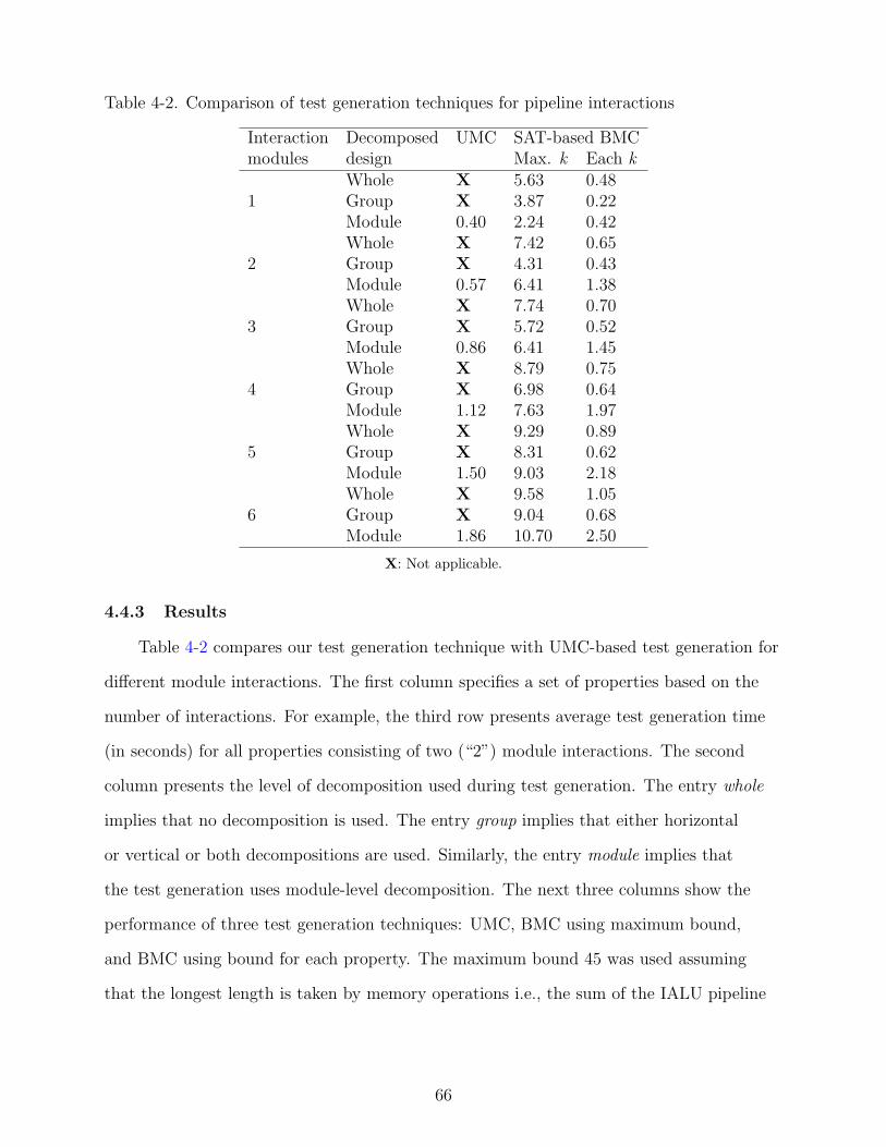
Table 4-2. Comparison of test generation techniques for pipeline interactions
Interaction Decomposed UMC SAT-based BMCmodules design Max. k Each k
Whole X 5.63 0.481 Group X 3.87 0.22
Module 0.40 2.24 0.42Whole X 7.42 0.65
2 Group X 4.31 0.43Module 0.57 6.41 1.38Whole X 7.74 0.70
3 Group X 5.72 0.52Module 0.86 6.41 1.45Whole X 8.79 0.75
4 Group X 6.98 0.64Module 1.12 7.63 1.97Whole X 9.29 0.89
5 Group X 8.31 0.62Module 1.50 9.03 2.18Whole X 9.58 1.05
6 Group X 9.04 0.68Module 1.86 10.70 2.50
X: Not applicable.
4.4.3 Results
Table 4-2 compares our test generation technique with UMC-based test generation for
different module interactions. The first column specifies a set of properties based on the
number of interactions. For example, the third row presents average test generation time
(in seconds) for all properties consisting of two (“2”) module interactions. The second
column presents the level of decomposition used during test generation. The entry whole
implies that no decomposition is used. The entry group implies that either horizontal
or vertical or both decompositions are used. Similarly, the entry module implies that
the test generation uses module-level decomposition. The next three columns show the
performance of three test generation techniques: UMC, BMC using maximum bound,
and BMC using bound for each property. The maximum bound 45 was used assuming
that the longest length is taken by memory operations i.e., the sum of the IALU pipeline
66

024681012
1 2 3 4 5 6Number of interactions
Gen
erat
ion
time
(sec
)
Max. bound without decomposition
Max. bound with decomposition
Individual bound without decomposition
Individual bound with decomposition
Figure 4-2. Test generation time comparison for four techniques
path length (5) and data-transfer path length (40). In the table, X indicates that a
counterexample was not found due to “Out of Memory” problem.
Figure 4-2 shows test generation time comparison for four techniques using: maximum
bound without decomposition, maximum bound with decomposition, individual bound
without decomposition, and individual bound with decomposition. As expected, Table 4-2
and Figure 4-2 show that the test generation time grows with the increase of the number
of module interactions. UMC can be used only with module level decompositions while
SAT-based BMC can be used without decomposition. Bound for each property reduces
approximately 90% of the test generation time compared to using BMC with maximum
bound. An interesting observation is that UMC with module level decomposition provides
better performance than SAT-based BMC. This is because the time to unfold the model
and convert it to a SAT problem is more than the time to search for a counterexample.
67

4.5 Chapter Summary
We presented a directed test generation technique for pipelined processors using
SAT-based bounded model checking. We developed a technique to convert pipeline
interaction faults into temporal logic properties. We presented a procedure for determining
bound for each property. We also developed a method for decomposing design and
properties in the context of SAT-based BMC. Our experimental results using MIPS
processor demonstrated that the test generation time using our technique is an order-of-magnitude
better compared to UMC-based or SAT-based BMC with maximum bound.
68

CHAPTER 5FUNCTIONAL TEST COMPACTION
In the current industrial practice, random and biased-random test generation
techniques at architecture (ISA) level are most widely used for simulation-based validation
to uncover errors early in the design cycle [2, 100]. Although directed tests require a
smaller test set compared to random tests for the same functional coverage goal, the
number of directed tests can still be extremely large. Therefore, there is a need for
functional test compaction techniques. Since a test generated for activating a particular
functional fault goes through pipeline paths over multiple clock cycles, there is a high
probability that the test can accompany multiple pipeline interactions before and after
it reaches the state that it tries to activate. We present an efficient test compaction
technique to significantly reduce the functional test set for validation of pipelined
processors.
Figure 5-1 shows the overall flow of our proposed test compaction methodology.
Using the specification of a processor, we create a finite state machine (FSM) model of
the processor and an FSM coverage metric based on pipeline interactions. Each FSM
state (transition) indicates a pipeline interaction and can be represented as a property for
test generation. FSM compaction is performed before test generation by eliminating the
states and the transitions that are illegal, redundant, or unreachable for the given design
constraints. Properties for the remaining states (after elimination) can be automatically
generated from the FSM model of the processor. Test programs to exercise the states in
the FSM model are produced using the model checking-based test generation technique.
Once all the tests are generated, test compaction is performed by pruning redundant test
programs to reduce the size of a test set.
The proposed method makes three important contributions. First, we propose an
efficient FSM model of the pipelined processors, and define FSM state and transition
coverage based on the pipeline interactions. Second, we propose an efficient compaction
69

Processor FSM model
FSM state/transition compaction
Directedtest generation
Covered all statesand transition?
Test compaction
Yes
No
Property for each state/transition
Reduced tests
Processor specification
FSM stateand transition
coverage
Figure 5-1. Functional test compaction methodology
technique to significantly reduce FSM states/transitions. Finally, we apply existing test
matrix reduction and minimization techniques to further reduce the number of directed
tests.
5.1 Related Work
Several FSM model-based test generation methodologies [24, 59, 65, 115] have
been developed for validation of pipelined processors where an FSM model is used to
generate a test suite based on FSM coverage metrics such as state, transition, or path
coverage. In modern processor designs, complicated micro-architectural mechanisms
include interactions among many pipeline stages and buffers that can lead the FSM-based
approaches to the state space explosion problem. To alleviate the state explosion, FSM
abstraction techniques [89, 99, 109] have been presented. However, these techniques use
70
reverse engineering to derive an FSM model from its RTL implementation because there
is a lack of a golden reference model. We propose a specification-driven FSM modeling
technique.
Due to the large volume of test data and the extremely long test time for manufacturing
test, considerable research has been done to reduce the structural test data volume. Test
compaction techniques are generally categorized into dynamic and static compactions.
Dynamic compaction is applied during test generation while static compaction is applied
after test generation. Rudnick and Patel [96] have proposed dynamic test compaction
for sequential circuits using fault simulation and genetic algorithms. El-Maleh and Osais
[41] have presented decomposition-based static compaction algorithms where a test
vector is decomposed into atomic components and the test vector is eliminated if its
components can be all moved to other test vectors. Set covering has been applied to
static compaction procedures for combinational circuits using the fault detection matrix
[18, 45, 57]. Dimopoulos and Linardis [40] have modeled static compaction for sequential
circuits as a set-covering problem. The matrix reduction techniques [110] can be applied
to mitigate the complexity of set covering by eliminating redundant rows (faults) and
columns (test vectors) in the fault detection matrix.
Although a lot of structural test compaction techniques have been proposed in
manufacturing test domain, there has been no work in functional test compaction in
validation domain since functional redundancy can be hard to find among functional
tests. Since the volume of functional tests can be extremely large even for directed tests,
we propose a functional test compaction methodology to reduce overall processor design
validation efforts.
5.2 FSM Modeling
Many works [28, 56, 75, 98] have been done on FSM modeling of processors as
bottom-up approaches where an abstract FSM model is extracted from RTL designs for
formal verification and test generation. However, in addition to difficulty in creating an
71
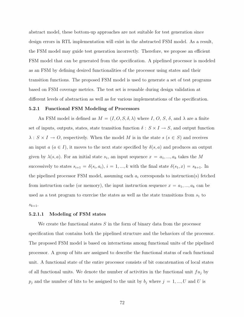
abstract model, these bottom-up approaches are not suitable for test generation since
design errors in RTL implementation will exist in the abstracted FSM model. As a result,
the FSM model may guide test generation incorrectly. Therefore, we propose an efficient
FSM model that can be generated from the specification. A pipelined processor is modeled
as an FSM by defining desired functionalities of the processor using states and their
transition functions. The proposed FSM model is used to generate a set of test programs
based on FSM coverage metrics. The test set is reusable during design validation at
different levels of abstraction as well as for various implementations of the specification.
5.2.1 Functional FSM Modeling of Processors
An FSM model is defined as M = (I, O, S, δ, λ) where I, O, S, δ, and λ are a finite
set of inputs, outputs, states, state transition function δ : S × I → S, and output function
λ : S × I → O, respectively. When the model M is in the state s (s ∈ S) and receives
an input a (a ∈ I), it moves to the next state specified by δ(s, a) and produces an output
given by λ(s, a). For an initial state s1, an input sequence x = a1, ..., ak takes the M
successively to states si+1 = δ(si, ai), i = 1, ..., k with the final state δ(s1, x) = sk+1. In
the pipelined processor FSM model, assuming each ai corresponds to instruction(s) fetched
from instruction cache (or memory), the input instruction sequence x = a1, ..., ak can be
used as a test program to exercise the states as well as the state transitions from s1 to
sk+1.
5.2.1.1 Modeling of FSM states
We create the functional states S in the form of binary data from the processor
specification that contains both the pipelined structure and the behaviors of the processor.
The proposed FSM model is based on interactions among functional units of the pipelined
processor. A group of bits are assigned to describe the functional status of each functional
unit. A functional state of the entire processor consists of bit concatenation of local states
of all functional units. We denote the number of activities in the functional unit fuj by
pj and the number of bits to be assigned to the unit by bj where j = 1, ..., U and U is
72

the number of functional units in the processor. Therefore, the total number of bits to
describe the processor FSM states is N =∑U
j=1 bj. We denote the number of states in the
machine M by NS = |S| = 2N . The state of functional unit fuj is denoted as ssj using
bj bits and the state sk of the processor FSM can be defined by concatenating ss1, ss2, ...,
ssU .
WB
…MEM IFID
Bit: BN B(N-1) … … B4 B3 B2 B1Figure 5-2. Binary format of the states in FSM model
For example, we assign two bits to represent four functional states of Fetch unit: ‘00’
for idle, ‘01’ for instruction fetch, ‘10’ for stall, and ‘11’ for exception. Figure 5-2 shows an
example of the FSM states of the pipelined processor. Given that all the functional units
have only four possible states, each unit requires 2 bits for its four functionalities. This
binary format of functional FSM model provides an efficient indexing mechanism to access
and analyze each functional state. In addition, next states can be described as Boolean
functions. For example, assuming the state transitions (si, sj) and (si, sk) with sj = ‘0011’
and sk = ‘0010’, the next states of si are expressed as B̄4B̄3B2B1 + B̄4B̄3B2B̄1 = B̄4B̄3B2.
For each state, a list of the next states are produced by transition functions described in
the following section.
5.2.1.2 Modeling of FSM state transitions
In this section, we describe the state transition functions based on the pipelining
behavior of the processor and the functional decomposition of the processor FSM into
smaller FSMs at unit level. The pipelining behaviors are the rules in each pipeline stage
that determine when instructions can move to the next stage and when they cannot. Since
not all the functional units affect the next state of other functional units, the transition
functions of the FSM can be decomposed into sub-functions each of which is dedicated to
a specific functional unit.
73
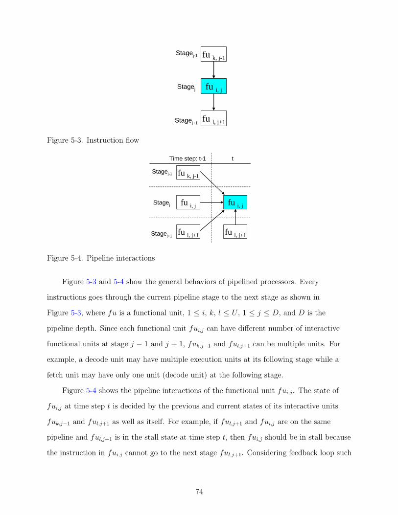
fu k, j-1
fu i, j
fu l, j+1
Stagej-1
Stagej
Stagej+1
Figure 5-3. Instruction flow
fu k, j-1
fu i, j
fu l, j+1
Stagej-1
Stagej
Stagej+1
fu i, j
fu l, j+1
Time step: t-1 t
Figure 5-4. Pipeline interactions
Figure 5-3 and 5-4 show the general behaviors of pipelined processors. Every
instructions goes through the current pipeline stage to the next stage as shown in
Figure 5-3, where fu is a functional unit, 1 ≤ i, k, l ≤ U , 1 ≤ j ≤ D, and D is the
pipeline depth. Since each functional unit fui,j can have different number of interactive
functional units at stage j − 1 and j + 1, fuk,j−1 and ful,j+1 can be multiple units. For
example, a decode unit may have multiple execution units at its following stage while a
fetch unit may have only one unit (decode unit) at the following stage.
Figure 5-4 shows the pipeline interactions of the functional unit fui,j. The state of
fui,j at time step t is decided by the previous and current states of its interactive units
fuk,j−1 and ful,j+1 as well as itself. For example, if ful,j+1 and fui,j are on the same
pipeline and ful,j+1 is in the stall state at time step t, then fui,j should be in stall because
the instruction in fui,j cannot go to the next stage ful,j+1. Considering feedback loop such
74

as data forwarding in the pipelined processor, fui,j at t will be also affected by the state of
fui,j+α at (t− 1) where 0 ≤ α ≤ D.
Based on the pipelining behavior, the state transition to the functional unit fui,j at
time step t is defined as ssi,j(t) = f(ssk,j−1(t − 1), ssi,j(t − 1), ssl,j+1(t − 1), ssl,j+1(t)).
Here, ssi,j(t) represents a set of bits to describe the functional state of fui,j at time step t,
and f represents a transition function decided by interactive units. Therefore, the state s
of the processor FSM can be expressed by concatenating ssi,j where i = 1, ..., U and 1 ≤ j
≤ D.
5.2.2 Functional Coverage of FSM Model
State coverage and transition coverage are most widely used as a coverage metric of
FSM models to generate a test set. State coverage ensures that every state of an FSM has
been visited. Transition (arc) coverage ensures that every transition between FSM states
has been traversed.
Assuming that each state transition occurs on the basis of clock cycle, the state
coverage of the proposed FSM model is similar to the pipeline interaction coverage at a
given clock cycle because an FSM state consists of the states of each functional unit. The
test program that covers the state will activate the corresponding pipeline interaction.
We can compute the number of theoretically possible FSM states based on the number of
functional units in the processor model and the average number of activities at each unit.
In general, the number of activities for a unit will be different based on what activities
we want to test. Furthermore, the number of activities varies for different units, thereby
each unit may require different number of bits for its functional states. Considering an
FSM model with m units where each unit can have on average p activities, the FSM will
have pm states which can be extremely large even for simple processors. For example, a
simple MIPS processor [54] with 10 functional units and 4 activities has approximately one
million states. This theoretical number of functional states can be reduced by eliminating
unreachable states using functional constraints described in the processor specification.
75

A test suite generated for the state coverage can successfully be used to reveal design
bugs during simulation-based validation. However, the state coverage has many holes
that represent functional behaviors and the hard-to-find bugs typically reside in state
transitions. Based on the state transition functions described in Section 5.2.1.2, each
state has a list of their next states. When a test visits the state and goes to one of its
next state, we put the next state off the list since the transition between the two states
is covered. State transition coverage of the FSM is achieved when the next state lists for
every states are empty. The number of state transitions is determined by the processor’s
functional behaviors. Theoretically, The maximum number of state transitions is N2,
where N is the number of states, and any state can go to any state.
5.3 Compaction before Test Generation
The state and transition compaction of an FSM plays a major role in efficient test
generation since reduction of one state or transition implies one less test vector to generate
and apply on the RTL implementation. The basic idea is to identify and eliminate all the
unreachable and redundant states as well as transitions with respect to coverage-driven
test generation.
5.3.1 Identifying Unreachable States
We use functional constraints described in the processor specification to distinguish
unreachable states from reachable ones. The constraints are represented as binary patterns
of FSM states. The states of those patterns are removed from the FSM and they are
not considered during test generation and coverage analysis since they are unreachable.
For example, for single instruction issue constraint at Issue stage with only one pipeline
register, if there are two following parallel execution pipelines EX1 and EX2, both
execution units cannot be in normal operation at the same time since this behavior is
illegal due to the single issue restriction. Assuming that EX1 and EX2 correspond to
the state variables B6B5 and B4B3 respectively in an 8-bit FSM, the binary pattern
‘xx0101xx’ represents unreachable states for the single issue constraint, where ‘01’
76
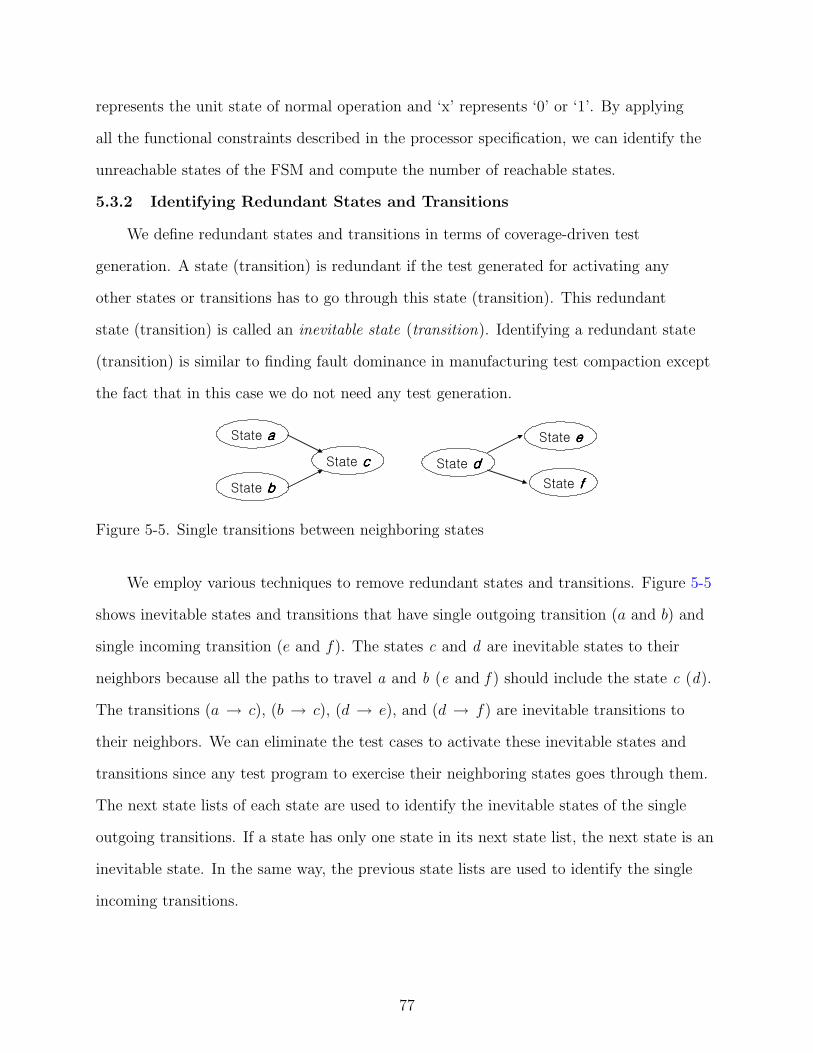
represents the unit state of normal operation and ‘x’ represents ‘0’ or ‘1’. By applying
all the functional constraints described in the processor specification, we can identify the
unreachable states of the FSM and compute the number of reachable states.
5.3.2 Identifying Redundant States and Transitions
We define redundant states and transitions in terms of coverage-driven test
generation. A state (transition) is redundant if the test generated for activating any
other states or transitions has to go through this state (transition). This redundant
state (transition) is called an inevitable state (transition). Identifying a redundant state
(transition) is similar to finding fault dominance in manufacturing test compaction except
the fact that in this case we do not need any test generation.
State aaaa
State bbbb
State cccc
State eeee
State ffff
State dddd
Figure 5-5. Single transitions between neighboring states
We employ various techniques to remove redundant states and transitions. Figure 5-5
shows inevitable states and transitions that have single outgoing transition (a and b) and
single incoming transition (e and f). The states c and d are inevitable states to their
neighbors because all the paths to travel a and b (e and f ) should include the state c (d).
The transitions (a → c), (b → c), (d → e), and (d → f) are inevitable transitions to
their neighbors. We can eliminate the test cases to activate these inevitable states and
transitions since any test program to exercise their neighboring states goes through them.
The next state lists of each state are used to identify the inevitable states of the single
outgoing transitions. If a state has only one state in its next state list, the next state is an
inevitable state. In the same way, the previous state lists are used to identify the single
incoming transitions.
77

5.3.3 Identifying Illegal State Transitions
The processor specification provides the rules in each pipeline unit when instructions
can move to the next stage and when they cannot. Our technique to identify illegal state
transitions is based on the rules in each functional unit and the composition of sub-state
transitions at unit level into processor state transitions as described in Section 5.2.1.2.
For example, if the state of the functional unit ssi,j is in normal operation at time t, then
the state of the previous stage unit ssk,j−1 cannot be in idle state at time t − 1 since the
instruction in fui,j must be ready at the previous pipeline stage at time t− 1.
Table 5-1. Transition rules between ssk,j−1(t− 1) and ssi,j(t)
ssk,j−1(t− 1) ssi,j(t)idle idle, stallnormal op. normal op., stall, exceptionstall idle, stallexception idle, stall
Table 5-2. Transition rules between ssi,j(t− 1) and ssi,j(t)
ssi,j(t− 1) ssi,j(t)idle idle, normal op., stall, exceptionnormal op. idle, normal op., exceptionstall idle, normal op., stall, exceptionexception idle
Table 5-3. Transition rules between ssl,j+1(t− 1) and ssi,j(t)
ssl,j+1(t− 1) ssi,j(t)idle idle, normal op., stall, exceptionnormal op. idle, normal op., stall, exceptionstall idle, normal op., stall, exceptionexception idle
Sub-state transition rules between interactive units are presented in the following
tables assuming four functional activities at each unit and one register between consecutive
pipeline stages. For example, in Table 5-1, if ssk,j−1(t − 1) = stall, then ssi,j(t) can be
either in idle or stall state because no instruction moves from the previous stage. In
Table 5-2 and Table 5-3, if ssk,j−1(t − 1) or ssl,j+1(t − 1) = exception, then ssi,j(t) should
be the idle state to flush the following instructions in the pipeline.
78

5.4 FSM Coverage-directed Test Generation
Model checking is very promising for directed test generation. In this approach, each
state and their transitions are converted into temporal properties. Instead of using the
properties, their negated version is applied to a model checker such that the model checker
produces a counterexample automatically. The counterexample contains a sequence of
instructions (test program) from an initial state to the state where the negated version of
the property fails.
5.4.1 Test Generation for State Coverage
An FSM state is composed of the sub-states of all functional units. We convert each
state into a linear temporal logic (LTL) property [35] where each property consists of
sub-states, temporal operators (G,F, X, U), and Boolean connectives (∧, ∨, ¬, and →).
Since pipeline interactions at a given cycle are semantically explicit and our processor
model is organized as structure-oriented functional units, each state can be converted
in the form of a property F (p1 ∧ p2 ∧ . . . ∧ pU ∧ (clk = t)) that combines activities pi
at i -th unit over U functional units at time step t. The negation of the property results
in G(¬p1 ∨ ¬p2 ∨ . . . ∨ ¬pU ∨ (clk 6= t)) that is applied to a model checker for test
generation.
For example, in order to generate a test for a 4-bit FSM state sj = ‘0011’ that has
2-bit sub-states ss1 and ss2 for two functional units, the property of the state is described
as F (ss1 = ‘00’ ∧ ss2 = ‘11’ ∧ (clk = t)) and its negated property G(ss1 6= ‘00’ ∨ ss2 6=‘11’ ∨ (clk 6= t)) is applied to generate a test program that activates the state sj at time t.
5.4.2 Test Generation for Transition Coverage
Using the state transition functions described in Section 5.2.1.2, the next state can be
expressed in the same form of the current state as p1’ ∧ p2’ ∧ . . . ∧ pU ’ ∧ (clk = t + 1).
Temporal operator X is used to describe the state transition between two consecutive
states where Xp means that p holds at next time step. We convert each state transition in
the form of a property F ((p1 ∧ p2 ∧ . . . ∧ pU ∧ (clk = t)) → X(p1’ ∧ p2’ ∧ . . . ∧ pU ’ ∧
79
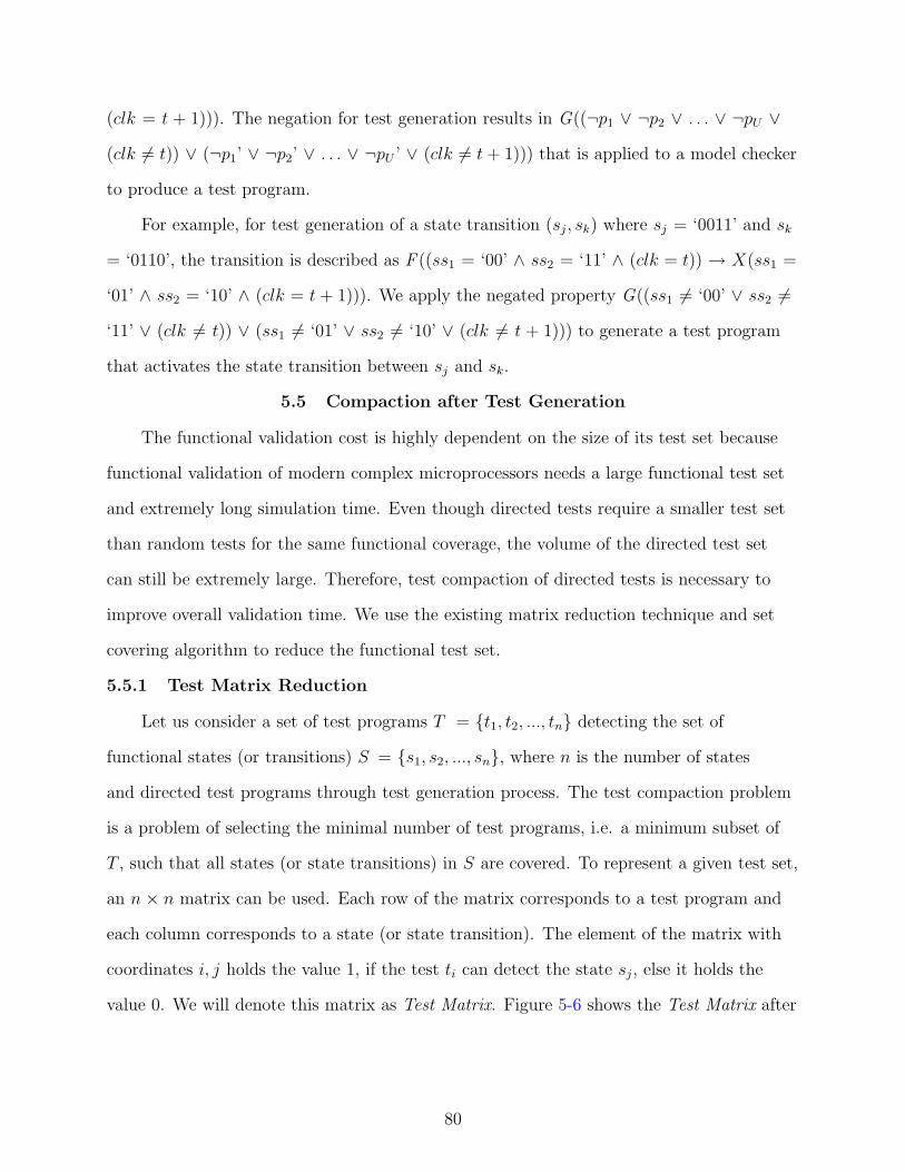
(clk = t + 1))). The negation for test generation results in G((¬p1 ∨ ¬p2 ∨ . . . ∨ ¬pU ∨(clk 6= t)) ∨ (¬p1’ ∨ ¬p2’ ∨ . . . ∨ ¬pU ’ ∨ (clk 6= t + 1))) that is applied to a model checker
to produce a test program.
For example, for test generation of a state transition (sj, sk) where sj = ‘0011’ and sk
= ‘0110’, the transition is described as F ((ss1 = ‘00’ ∧ ss2 = ‘11’ ∧ (clk = t)) → X(ss1 =
‘01’ ∧ ss2 = ‘10’ ∧ (clk = t + 1))). We apply the negated property G((ss1 6= ‘00’ ∨ ss2 6=‘11’ ∨ (clk 6= t)) ∨ (ss1 6= ‘01’ ∨ ss2 6= ‘10’ ∨ (clk 6= t + 1))) to generate a test program
that activates the state transition between sj and sk.
5.5 Compaction after Test Generation
The functional validation cost is highly dependent on the size of its test set because
functional validation of modern complex microprocessors needs a large functional test set
and extremely long simulation time. Even though directed tests require a smaller test set
than random tests for the same functional coverage, the volume of the directed test set
can still be extremely large. Therefore, test compaction of directed tests is necessary to
improve overall validation time. We use the existing matrix reduction technique and set
covering algorithm to reduce the functional test set.
5.5.1 Test Matrix Reduction
Let us consider a set of test programs T = {t1, t2, ..., tn} detecting the set of
functional states (or transitions) S = {s1, s2, ..., sn}, where n is the number of states
and directed test programs through test generation process. The test compaction problem
is a problem of selecting the minimal number of test programs, i.e. a minimum subset of
T , such that all states (or state transitions) in S are covered. To represent a given test set,
an n × n matrix can be used. Each row of the matrix corresponds to a test program and
each column corresponds to a state (or state transition). The element of the matrix with
coordinates i, j holds the value 1, if the test ti can detect the state sj, else it holds the
value 0. We will denote this matrix as Test Matrix. Figure 5-6 shows the Test Matrix after
80
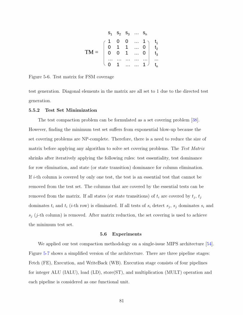
s1 s2 s3 … sn
1 0 0 … 1 t10 1 1 … 0 t20 0 1 … 0 t3… … … … … ...0 1 … … 1 tn
TM =
Figure 5-6. Test matrix for FSM coverage
test generation. Diagonal elements in the matrix are all set to 1 due to the directed test
generation.
5.5.2 Test Set Minimization
The test compaction problem can be formulated as a set covering problem [38].
However, finding the minimum test set suffers from exponential blow-up because the
set covering problems are NP-complete. Therefore, there is a need to reduce the size of
matrix before applying any algorithm to solve set covering problems. The Test Matrix
shrinks after iteratively applying the following rules: test essentiality, test dominance
for row elimination, and state (or state transition) dominance for column elimination.
If i-th column is covered by only one test, the test is an essential test that cannot be
removed from the test set. The columns that are covered by the essential tests can be
removed from the matrix. If all states (or state transitions) of ti are covered by tj, tj
dominates ti and ti (i-th row) is eliminated. If all tests of si detect sj, sj dominates si and
sj (j-th column) is removed. After matrix reduction, the set covering is used to achieve
the minimum test set.
5.6 Experiments
We applied our test compaction methodology on a single-issue MIPS architecture [54].
Figure 5-7 shows a simplified version of the architecture. There are three pipeline stages:
Fetch (FE), Execution, and WriteBack (WB). Execution stage consists of four pipelines
for integer ALU (IALU), load (LD), store(ST), and multiplication (MULT) operation and
each pipeline is considered as one functional unit.
81
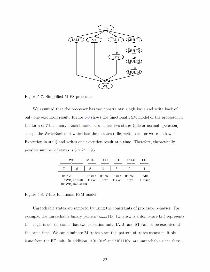
FE
LD1IALU ST
LD2
WB
MULT1
MULT3
MULT2
MULT4
Figure 5-7. Simplified MIPS processor
We assumed that the processor has two constraints: single issue and write back of
only one execution result. Figure 5-8 shows the functional FSM model of the processor in
the form of 7-bit binary. Each functional unit has two states (idle or normal operation)
except the WriteBack unit which has three states (idle, write back, or write back with
Execution in stall) and writes one execution result at a time. Therefore, theoretically
possible number of states is 3× 25 = 96.
7 6 5 4 3 2 1
FEIALUSTLDMULTWB
0: idle1: issue
0: idle1: exe
0: idle1: exe
0: idle1: exe
0: idle1: exe
00: idle01: WB, no stall10: WB, stall at EX
Figure 5-8. 7-bits functional FSM model
Unreachable states are removed by using the constraints of processor behavior. For
example, the unreachable binary pattern ‘xxxx11x’ (where x is a don’t-care bit) represents
the single issue constraint that two execution units IALU and ST cannot be executed at
the same time. We can eliminate 24 states since this pattern of states means multiple
issue from the FE unit. In addition, ‘101101x’ and ‘101110x’ are unreachable since these
82

patterns are only possible in dual issue scenario. After removing all unreachable states,
the number of states to be considered is reduced to 57 (41% reduction). For FSM state
compaction, we searched for incoming and outgoing single transitions that have inevitable
states to their neighbors to travel to other states. We do not need to generate a test for
those states since one or more test programs to exercise their neighbors will cover them.
After state compaction, we could reduce the number of tests by 6 (11% reduction). As
a result, the number of directed test programs required for the state coverage is 51. Our
framework generated 51 tests using model checking. After applying test matrix reduction
technique on these 51 tests, 26 essential tests are identified. Set covering produced another
3 tests in the matrix. As a result, the total number of tests is 29 (70% overall reduction)
to cover all the states of the MIPS processor.
So far we discussed the test compaction in the context of FSM states. In the
remainder of this section, we present the results for test compaction using FSM transitions.
Unless we apply our test compaction technique we need to generate test for 3249 (57× 57)
transitions since there are 57 valid states. Clearly, each state cannot have transition to
all other states. Once we apply the elimination technique described in Section 5.3.3, our
framework identifies 2793 illegal transitions (86% reduction) and thereby only 456 valid
transitions are left. In other words, only 456 test vectors are sufficient to cover all the
transitions in the MIPS processor. This can be improved further by applying matrix
reduction and set covering techniques. However, the number of final required tests depend
on the length of each test. If each test tries to cover a longest path in the transition
diagram, only 44 (overall 99% reduction) tests will be required. However, a model checker
typically uses the shortest possible test to activate the required transition which can lead
to any number between 44 and 456. Therefore, our approach can generate 86-99% overall
reduction in functional tests without sacrificing functional coverage.
83

5.7 Chapter Summary
This chapter presented a functional test compaction methodology that can significantly
reduce the number of directed tests without sacrificing the functional coverage. Our test
compaction technique made three important contributions. First, it proposed a simple
FSM model of the pipelined processors and defined FSM state and transition coverage
based on pipeline interactions. Second, we proposed an FSM state/transition reduction
technique to eliminate the redundant states/transitions that can be covered by the
remaining states/transitions with respect to test generation. This leads to reduction
on directed tests since each state/transition in the FSM corresponds to a directed test.
Finally, we used existing test matrix reduction and minimization techniques to further
reduce the number of directed tests. Our experimental results using a simple MIPS
processor demonstrated an overall 86-99% reduction of functional tests.
84
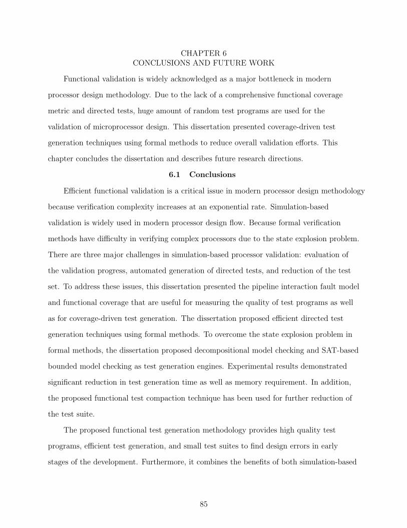
CHAPTER 6CONCLUSIONS AND FUTURE WORK
Functional validation is widely acknowledged as a major bottleneck in modern
processor design methodology. Due to the lack of a comprehensive functional coverage
metric and directed tests, huge amount of random test programs are used for the
validation of microprocessor design. This dissertation presented coverage-driven test
generation techniques using formal methods to reduce overall validation efforts. This
chapter concludes the dissertation and describes future research directions.
6.1 Conclusions
Efficient functional validation is a critical issue in modern processor design methodology
because verification complexity increases at an exponential rate. Simulation-based
validation is widely used in modern processor design flow. Because formal verification
methods have difficulty in verifying complex processors due to the state explosion problem.
There are three major challenges in simulation-based processor validation: evaluation of
the validation progress, automated generation of directed tests, and reduction of the test
set. To address these issues, this dissertation presented the pipeline interaction fault model
and functional coverage that are useful for measuring the quality of test programs as well
as for coverage-driven test generation. The dissertation proposed efficient directed test
generation techniques using formal methods. To overcome the state explosion problem in
formal methods, the dissertation proposed decompositional model checking and SAT-based
bounded model checking as test generation engines. Experimental results demonstrated
significant reduction in test generation time as well as memory requirement. In addition,
the proposed functional test compaction technique has been used for further reduction of
the test suite.
The proposed functional test generation methodology provides high quality test
programs, efficient test generation, and small test suites to find design errors in early
stages of the development. Furthermore, it combines the benefits of both simulation-based
85
techniques and formal methods to reduce the overall effort for functional validation of
pipelined processors.
6.2 Future Research Directions
Automated coverage-driven test generation for validation of microprocessors is a
challenging problem. The work presented in this dissertation can be extended in the
following directions:
• Develop an efficient technique of clustering modules for decompositional modelchecking. Not all the properties described in temporal logic can be decomposed at themodule level. However, if the design is decomposed into several groups of modules,most of the properties can benefit from decompositional model checking.
• Find the bounds of counterexamples for SAT-based bounded model checking for otherfunctional fault models. Proper determination of the bounds for each property resultsin reduction of test generation time.
• Develop an algorithm to find the most effective test programs in a test set. Theyprobably contain complex combinations of pipeline interactions. Instead of findingan optimal test set which is NP problem, greedy approach can be applied to testcompaction methodology by identifying the most effective tests.
• Extend the proposed coverage-driven test generation methodology to SoC designvalidation which will have much more communication and interaction among itsfunctional units.
• Investigate relationship between functional verification and manufacturing testing.The goal is to reuse the common aspects of the two activities for improved functionalverification. For example, automatic test pattern generation (ATPG) can beguided (or even replaced) by the functional test programs generated for functionalverification. Similarly, the properties, constraints as well as the functional verificationenvironments can be used to guide ATPGs. Likewise, the manufacturing test patternscan be used in functional verification to improve functional coverage and reduceverification effort.
86

REFERENCES
[1] J. Abraham and W. Fuchs. Fault and error models for VLSI. Proc. of IEEE,74(5):639–654, 1986.
[2] A. Adir, E. Almog, L. Fournier, E. Marcus, M. Rimon, M. Vinov, and A. Ziv.Genesys-pro: Innovations in test program generation for functional processorverification. IEEE Design & Test of Computers, 21(2):84–93, 2004.
[3] A. Adir, S. Asaf, L. Fournier, I. Jaeger, and O. Peled. A framework for thevalidation of processor architecture compliance. In Proc. of Design AutomationConference (DAC), pages 902–905, 2007.
[4] A. Aharon, D. Goodman, M. Levinger, Y. Lichtenstein, Y. Malka, C. Metzger,M. Molcho, and G. Shurek. Test program generation for functional verification ofpowerpc processors in ibm. In Proc. of Design Automation Conference (DAC), pages279–285, 1995.
[5] R. Alur, R. K. Brayton, T. A. Henzinger, S. Qadeer, and S. K. Rajamani.Partial-order reduction in symbolic state-space exploration. Formal Methods inSystem Design, 18(2):97–116, 2001.
[6] R. Alur, K. McMillan, and D. Peled. Deciding global partial-order properties.Formal Methods in System Design, 26(1):7–25, 2005.
[7] N. Amla, X. Du, A. Kuehlmann, R. Kurshan, and K. McMillan. An analysis ofSAT-based model checking techniques in an industrial environment. In Conferenceon Correct Hardware Design and Verification Methods (CHARME), pages 254–268.Springer, 2005.
[8] N. Amla, R. Kurshan, K. McMillan, and R. Medel. Experiment analysis of differenttechniques for bounded model checkings. In Tools and Algorithms for the Analysisand Construction of Systems (TACAS), volume 2619 of LNCS, pages 34–48.Springer, 2003.
[9] Z. S. Andraus, M. H. Liffiton, and K. A. Sakallah. Refinement strategies forverification methods based on datapath abstraction. In Proc. of Asia South PacificDesign Automation Conference (ASPDAC), pages 19–24, 2006.
[10] Z. S. Andraus and K. A. Sakallah. Automatic abstraction and verification of verilogmodels. In Proc. of Design Automation Conference (DAC), pages 218–223, 2004.
[11] H. Azatchi, L. Fournier, E. Marcus, S. Ur, A. Ziv, and K. Zohar. Advancedanalysis techniques for cross-product coverage. IEEE Transactions on Computers,55(11):1367–1379, 2006.
[12] T. Basten, D. Bonacki, and M. Geilen. Cluster-based partial-order reduction.Automated Software Engineering, 11(4):365–402, 2004.
87

88
[13] M. Benjamin, D. Geist, A. Hartman, G. Mas, and R. Smeets. A study incoverage-driven test generation. In Proc. of Design Automation Conference (DAC),pages 970–975, 1999.
[14] B. Bentley. High level validation of next generation microprocessors. In Proceedingsof High Level Design Validation and Test (HLDVT), pages 31–35, 2002.
[15] A. Biere, A. Cimatti, and E. M. Clarke. Bounded model checking. Advances inComputers, 58, 2003.
[16] A. Biere, A. Cimatti, E. M. Clarke, and Y. Zhu. Symbolic model checking withoutBDDs. In Tools and Algorithms for the Analysis and Construction of Systems(TACAS), volume 1579 of LNCS, pages 193–207. Springer, 1999.
[17] P. Bjesse and J. Kukula. Using counter example guided abstraction refinement tofind complex bugs. In Proc. of Design Automation and Test in Europe (DATE), page10156, 2004.
[18] K. O. Boateng, H. Konishi, and T. Nakata. A method of static compaction of teststimuli. In Proceedings of Asian Test Symposium (ATS), pages 137–142, 2001.
[19] R. Bryant. Graph-Based Algorithms for Boolean Function Manipulation. IEEETrans. Computers, C-35(8):677–691, August 1986.
[20] R. E. Bryant. A methodology for hardware verification based on logic simulation.Journal of the ACM (JACM), 38(2):299–328, 1991.
[21] R. E. Bryant. Symbolic simulation techniques and applications. In Proc. of DesignAutomation Conference (DAC), pages 517–521, 1991.
[22] J. R. Burch, E. M. Clarke, and K. L. McMillan. Symbolic model checking: 1020
states and beyond. Information and Computation, 98:142–170, 1992.
[23] M. L. Bushnell and V. D. Agrawal. Essentials of Electronic Testing for Digital,Memory and Mixed-Signal VLSI Circuits. Kluwer Academic Publishers, Boston, MA,2000.
[24] D. Campenhout, T. Mudge, and J. Hayes. High-level test generation for designverification of pipelined microprocessors. In Proc. of Design Automation Conference(DAC), pages 185–188, 1999.
[25] P. Camurati and P. Prinetto. Formal verification of hardware correctness:Introduction and survey of current research. IEEE Computer, 21(7):8–19, 1988.
[26] S. Chakravarty and P. J. Thadikaran. Introduction to IDDQ Testing. KluwerAcademic Publishers, Boston, MA, 1997.
[27] K.-T. Cheng and J.-Y. Jou. A functional fault model for sequential machines. IEEETransactions on Computer-Aided Design, 11(9):1065.1073, 1992.

89
[28] K.-T. Cheng and A. S. Krishnakumar. Automatic generation of functional vectorsusing the extended finite state machine model. ACM Transactions on DesignAutomation of Electronic Systems (TODES), 1(1):57–79, 1996.
[29] A. Cimatti, E. M. Clarke, F. Giunchiglia, and M. Roveri. NUSMV: A new symbolicmodel verifier. In Proc. of Intl. Conference on Computer Aided Verification (CAV),volume 1633 of LNCS, pages 495–499. Springer, 1999.
[30] E. M. Clarke, A. Biere, R. Ramimi, and Y. Zhu. Bounded model checking usingsatisfiability solving. Formal Methods in System Design (FMSD), 19(1):7–34, 2001.
[31] E. M. Clarke, T. Filkorn, and S. Jha. Exploiting symmetry in temporal logic modelchecking. In Proc. of International Conference on Computer Aided Verification(CAV), pages 450–462, 1993.
[32] E. M. Clarke, O. Grumberg, S. Jha, Y. Lu, and H. Veith. Counterexample-guidedabstraction refinement for symbolic model checking. Journal of the ACM (JACM),50(5):752–794, 2003.
[33] E. M. Clarke, O. Grumberg, and D. E. Long. Model checking and abstraction. ACMTransactions on Programming Languages and Systems (TOPLAS), 16(5):1512–1542,1994.
[34] E. M. Clarke, O. Grumberg, K. L. McMillan, and X. Zhao. Efficient generationof counterexamples and witnesses in symbolic model checking. In Proc. of DesignAutomation Conference (DAC), pages 427–432, 1995.
[35] E. M. Clarke, O. Grumberg, and D. A. Peled. Model Checking. MIT Press,Cambridge, MA, 1999.
[36] E. M. Clarke, H. Jain, and D. Kroening. Verification of specc using predicateabstraction. Formal Methods in System Design, 30(1):5–28, 2007.
[37] F. Copty, L. Fix, R. Fraer, E. Giunchiglia, G. Kamhi, A. Tacchella, and M. Y.Vardi. Benefits of bounded model checking at an industrial setting. In Proc. of Intl.Conference on Computer Aided Verification (CAV), LNCS, pages 436–453. Springer,2001.
[38] F. Corno, P. Prinetto, M. Rebaudengo, and M. S. Reorda. New static compactiontechniques of test sequences for sequential circuits. In Proc. of European Conferenceon Design and Test (ED&TC)), pages 37–43, 1997.
[39] P. Cousot and R. Cousot. Abstract interpretation: A unified lattice model for staticanalysis of programs by construction or approximation of fixpoints. In Proc. of theACM Symposium on Principles of Programming Languages, pages 238–252, 1997.
[40] M. Dimopoulos and P. Linardis. Efficient static compaction of test sequence setsthrough the application of set covering techniques. In Proc. of Design Automationand Test in Europe (DATE), page 10194, 2004.
90
[41] A. H. El-Maleh and Y. E. Osais. Test vector decomposition-based static compactionalgorithms for combinational circuits. ACM Transactions on Design Automation ofElectronic Systems, 8(4):430–459, 2003.
[42] E. Emerson and R. Trefler. From asymmetry to full symmetry: New techniques forsymmetry reduction in model checking. In Proc. of Correct Hardware Design andVerification Methods (CHARME), volume 1703 of LNCS, pages 142–156. Springer,1999.
[43] S. Ezer and S. Johnson. Smart diagnostics for configurable processor verification. InProc. of Design Automation Conference (DAC), pages 789–794, 2005.
[44] S. Fine and A. Ziv. Coverage directed test generation for functional verificationusing bayesian networks. In Proc. of Design Automation Conference (DAC), pages286–291, 2003.
[45] P. F. Flores, H. C. Neto, and J. P. Marques-Silva. On applying set coveringmodels to test set compaction. In Proceedings of Great Lakes Sympoisum on VLSI(GLSVLSI), pages 8–11, 1999.
[46] L. Fournier, A. Koyfman, and M. Levinger. Developing an architecture validationsuite: application to the powerpc architecture. In Proc. of Design AutomationConference (DAC), pages 189–194, 1999.
[47] A. Gargantini and C. Heitmeyer. Using model checking to generate tests fromrequirements specifications. In ACM SIGSOFT Software Engineering Notes,volume 24, pages 146–162, 1999.
[48] A. Gluska. Practical methods in coverage-oriented verification of the merommicroprocessor. In Proc. of Design Automation Conference (DAC), pages 332–337,2006.
[49] P. Godefroid, D. Peled, and M. Staskauskas. Using partial-order methods in theformal validation of industrial concurrent programs. In Proc. of InternationalSymposium on Software Testing and Analysis (ISSTA), pages 261–269, 1996.
[50] E. Goldberg and Y. Novikov. BerkMin: a fast and robust SAT-solver. In Proc. ofDesign Automation and Test in Europe (DATE), pages 142–149, 2002.
[51] R. Grinwald, E. Harel, M. Orgad, S. Ur, and A. Ziv. User defined coverage - Atool supported methodology for design verification. In Proc. of Design AutomationConference (DAC), pages 158–163, 1998.
[52] S. Gurumurthy, S. Vasudevan, and J. A. Abraham. Automated mapping ofpre-computed module-level test sequences to processor instructions. In Proc. ofIntl. Test Conference (ITC), 2005.
[53] I. G. Harris. A coverage metric for the validation of interacting processes. In Proc.of Design Automation and Test in Europe (DATE), pages 1019–1024, 2006.
91
[54] J. Hennessy and D. Patterson. Computer Architecture: A Quantitative Approach.Morgan Kaufmann, Sanfrancisco, CA, 2003.
[55] P. Ho, A. Isles, and T. Kam. Formal verification of pipeline control using controlledtoken nets and abstract interpretation. In Proc. of International Conference onComputer-Aided Design (ICCAD), pages 529–536, 1998.
[56] R. C. Ho, C. H. Yang, M. A. Horowitz, and D. L. Dill. Architecture validation forprocessors. In Proc. International Symposium on Computer Architecture (ISCA),pages 404–413, 1995.
[57] D. S. Hochbaum. An optimal test compression procedure for combinational circuits.IEEE Transactions on Computer-Aided Design of Integrated Circuits and Systems,15(10):1294–1299, 1996.
[58] http:www.freescale.com/files/32bit/doc/ref manual/e500CORERMAD.pdf.PowerPCTM e500 Core Family Reference Manual, 2006.
[59] H. Iwashita, S. Kowatari, T. Nakata, and F. Hirose. Automatic test programgeneration for pipelined processors. In Proc. International Conference on Computer-Aided Design (ICCAD), pages 580–583, 1994.
[60] C. Jacobi. Formal verification of complex out-of-order pipelines by combiningmodel checking and theorem proving. In E. Brinksma and K. Larsen, editor, Proc.of Computer Aided Verification (CAV), volume 2404 of LNCS, pages 309–323.Springer-Verlag, 2002.
[61] H. Jain, D. Kroening, N. Sharygina, and E. Clarke. Word level predicate abstractionand refinement for verifying rtl verilog. In Proc. of Design Automation Conference(DAC), pages 445–450, 2005.
[62] N. Jha and S. Gupta. Testing of Digital Systems. Cambridge University Press,Cambridge, United Kingdom, 2003.
[63] R. Jhala and K. L. McMillan. Microarchitecture verification by compositional modelchecking. In G. Berry et al., editor, Proc. of Computer Aided Verification (CAV),volume 2102 of LNCS, pages 396–410. Springer-Verlag, 2001.
[64] C. Kern and M. Greenstreet. Formal verification in hardware design: A survey. ACMTransactions on Design Automation of Electronic Systems (TODAES), 4(2):123–193,1999.
[65] K. Kohno and N. Matsumoto. A new verification methodology for complex pipelinebehavior. In Proc. of Design Automation Conference (DAC), pages 816–821, 2001.
[66] H.-M. Koo and P. Mishra. Functional coverage-driven test generation formicroprocessor verification. In Proc. of US-Korea Conference (UKC), pages 19–24,2006.
92
[67] H.-M. Koo and P. Mishra. Functional test generation using property decompositionsfor validation of pipelined processors. In Proc. of Design Automation and Test inEurope (DATE), pages 1240–1245, 2006.
[68] H.-M. Koo and P. Mishra. Test generation using (sat)-based bounded modelchecking for validation of pipelined processors. In Proc. of ACM Great LakesSymposium on VLSI (GSLVLSI), pages 362–365, 2006.
[69] H.-M. Koo and P. Mishra. Automated micro-architectural test generation forvalidation of modern processors. In Proc. of US-Korea Conference (UKC), pages25–30, 2007.
[70] H.-M. Koo, P. Mishra, J. Bhadra, and M. Abadir. Directed micro-architecturaltest generation for an industrial processor: A case study. In IEEE InternationalWorkshop on Microprocessor Test and Verification (MTV)), pages 33–36, 2006.
[71] S. Kripke. Semantic consideration on model logic. In Proc. of a Colloquium: Modaland Many valued Logics, pages 83–94, 1963.
[72] N. Krishnamurthy, A. K. Martin, M. S. Abadir, and J. A. Abraham. ValidatingPowerPC microprocessor custom memories. IEEE Design & Test, 17(4):61–76, 2000.
[73] A. Kuehlmann and F. Krohm. Equivalence checking using cuts and heaps. In Proc.of Design Automation Conference (DAC), pages 263–268, 1997.
[74] O. Lachish, E. Marcus, S. Ur, and A. Ziv. Hole analysis for functional coverage data.In Proc. of Design Automation Conference (DAC), pages 807–812, 2002.
[75] C. Liu, C.-C. Yen, and J.-Y. Jou. Automatic functional vector generation using theinteracting FSM model. In Proc. of International Symposium on Quality ElectronicDesign (ISQED), pages 372–377, 2001.
[76] F. Y. Mang and P.-H. Ho. Abstraction refinement by controllability andcooperativeness analysis. In Proc. of Design Automation Conference (DAC),pages 224–229, 2004.
[77] P. Manolios and S. K. Srinivasan. A complete compositional reasoning framework forthe efficient verification of pipelined machines. In Proc. of International Conferenceon Computer Aided Design (ICCAD), pages 863–870, 2005.
[78] J. P. Marques-Silva and K. A. Sakallh. GRASP: A search algorithm for propositionalsatisfiability. IEEE Transactions on Computers, 48(5):506–521, 1999.
[79] K. L. McMillan. SMV Model Checker, Cadence Berkeley Laboratory.http://embedded.eecs.berkeley.edu/Alumni/kenmcmil/smv, October, 2002.
[80] K. L. McMillan. Symbolic Model Checking: An Approach to the State ExplosionProblem. Kluwer Academic Publishers, Boston, MA, 1993.
93
[81] K. L. McMillan. Methods for exploiting SAT solvers in unbounded model checking.In Proceedings of MEMOCODE, pages 135–142, 2003.
[82] A. Miller, A. Donaldson, and M. Calder. Symmetry in temporal logic modelchecking. ACM Computing Surveys (CSUR), 38(3):1–36, 2006.
[83] P. Mishra and N. Dutt. Automatic Functional Test Program Generation forPipelined Processors using Model Checking. In Proc. of High Level Design Validationand Test (HLDVT), pages 99–103, 2002.
[84] P. Mishra and N. Dutt. Graph-based functional test program generation forpipelined processors. In Proc. of Design Automation and Test in Europe (DATE),pages 182–187, 2004.
[85] P. Mishra and N. Dutt. Functional coverage driven test generation for validation ofpipelined processors. In Proc. of Design Automation and Test in Europe (DATE),pages 678–683, 2005.
[86] P. Mishra and N. D. Dutt. Functional Verification of Programmable EmbeddedArchitectures: A Top-Down Approach. Springer Verlag, New York, NY, 2005.
[87] P. Mishra, H.-M. Koo, and Z. Huang. Language-driven validation of pipelinedprocessors using satisfiability solvers. In IEEE International Workshop on Micropro-cessor Test and Verification (MTV)), pages 119–126, 2005.
[88] M. H. Moskewicz, C. F. Madigan, Y. Zhao, L. Zhang, and S. Malik. Chaff:Engineering an efficient SAT solver. In Proc. of Design Automation Conference(DAC), pages 530–535, 2001.
[89] D. Moundanos, J. A. Abraham, and Y. V. Hoskote. Abstraction techniques forvalidation coverage analysis and test generation. IEEE Transactions on Computers,47(1):2–14, 1998.
[90] G. Parthasarathy, M. K. Iyer, K.-T. Cheng, and L.-C. Wang. Safety propertyverification using sequential sat and bounded model checking. IEEE Design & Testof Computers, 21(2):132–143, 2004.
[91] D. Peled. Using partial-order methods in the formal validation of industrialconcurrent programs. In Proc. of International Conference on Computer AidedVerification (CAV), pages 409–423, 1993.
[92] A. Piziali. Functional Verification Coverage Measurement and Analysis. KluwerAcademic Publishers, Boston, MA, 2004.
[93] M. R. Prasad, A. Biere, and A. Gupta. A survey of recent advances in SAT-basedformal verification. Intl. Journal on Software Tools for Technology Transfer (STTT),7(2):156–173, 2005.

94
[94] M. Puig-Medina, G. Ezer, and P. Konas. Verification of configurable processor cores.In Proc. of Design Automation Conference (DAC), pages 426–431, 2000.
[95] A. Roy, S. K. Panda, R. Kumar, and P. P. Chakrabarti. A framework for systematicvalidation and debugging of pipeline simulators. ACM Transactions on DesignAutomation of Electronic Systems (TODES), 10(3):462–491, 2005.
[96] E. M. Rudnick and J. H. Patel. Efficient techniques for dynamic test sequencecompaction. IEEE Transactions on Computers, 48(3):323–330, 1999.
[97] A. Sen. Error diagnosis in equivalence checking of high performance microprocessors.Electronic Notes in Theoretical Computer Science (ENTCS), 174(4):9–18, 2007.
[98] J. Shen and J. Abraham. Verification of processor microarchitectures. In Proc. ofVLSI Test Symposium (VTS), pages 189–194, 1999.
[99] J. Shen and J. A. Abraham. An RTL abstraction technique for processormicroarchitecture validation and test generation. Journal of Electronic Testing:Theory and Applications, 16(1-2):67–81, 2000.
[100] K. Shimizu, S. Gupta, T. Koyama, T. Omizo, J. Abdulhafiz, L. McConville, andT. Swanson. Verification of the cell broadband engine processor. In Proc. of DesignAutomation Conference (DAC), pages 338–343, 2006.
[101] A. P. Sistla and P. Godefroid. Symmetry and reduced symmetry in modelchecking. ACM Transactions on Programming Languages and Systems (TOPLAS),26(4):702–734, 2004.
[102] M. Srivas and M. Bickford. Formal verification of a pipelined microprocessor. IEEESoftware, 7(5):52–64, 1990.
[103] T. Schubert. High level formal verification of next generation microprocessors. InProceedings of Design Automation Conference (DAC), pages 1–6, 2003.
[104] S. Tasiran and K. Keutzer. Coverage metrics for functional validation of hardwaredesigns. IEEE Design & Test of Computers, 18(4):36–45, 2001.
[105] P. A. Thaker, V. D. Agrawal, and M. E. Zaghloul. Validation vector grade (VVG):A new coverage metric for validation and test. In Proc. of VLSI Test Symposium,pages 182–188, 1999.
[106] S. Thatte and J. Abraham. Test generation for microprocessors. IEEE Transactionson Computers, 29(6):429–441, 1980.
[107] C. Timoc, M. Buehler, T. Griswold, C. Pina, F. Stott, and L. Hess. Logical modelsof physical failures. In Proc. of International Test Conference (ITC), pages 546–553,1983.

95
[108] S. Ur and Y. Yadin. Micro architecture coverage directed generation of testprograms. In Proc. of Design Automation Conference (DAC), pages 175–180, 1999.
[109] N. Utamaphethai, R. D. S. Blanton, and J. P. Shen. Effectiveness ofmicroarchitecture test program generation. IEEE Design & Test, 17(4):38–49,2000.
[110] T. Villa, T. Kam, R. K. Brayton, and A. L. Sangiovanni-Vincentelli. Explicit andimplicit algorithms for binate covering problems. IEEE Transactions on Computer-Aided Design of Integrated Circuits and Systems, 16(7):677–691, 1997.
[111] R. L. Wadsack. Fault modeling and logic simulation of CMOS and MOS integratedcircuits. Bell System Technical Journal, 57(5):1449–1474, 1978.
[112] I. Wagner, V. Bertacco, and T. Austin. StressTest: an automatic approach to testgeneration via activity monitors. In Proc. of Design Automation Conference (DAC),pages 783–788, 2005.
[113] M. Wilding, D. Greve, and D. Hardin. Efficient simulation of formal processormodels. Formal Methods in System Design, 18(3):233–248, 2001.
[114] H. Zhang. SATO: An efficient propositional prover. In Proc. of InternationalConference on Automated Deduction (CADE), volume 1249 of LNCS, pages 272–275.Springer, 1997.
[115] Y. Zhang, D. Wang, J. Wang, and W. Zheng. Using model-based test programgenerator for simulation validation. In Embedded Software and Systems, volume 3605of LNCS, pages 549–556. Springer, 2005.
[116] A. Ziv. Cross-product functional coverage measurement with temporalproperties-based assertions. In Proc. of Design Automation and Test in Europe(DATE), pages 834–841, 2003.

BIOGRAPHICAL SKETCH
Heon-Mo Koo received his B.S. and M.S. degrees at the Department of Electronic
and Electric Engineering from Kyungpook National University in South Korea in 1993
and 1995 respectively. During M.S. studies, he developed digital image processing and
video compression algorithms. In 1995, he joined at LG Electronics Research Center in
Seoul, South Korea. As a senior research engineer, he worked on functional modeling
and validation of MPEG encoder/decoder, development of a RISC-type embedded
processor for MPEG decoder, and digital video processing and enhancement algorithms
for HDTV and DVD systems. Since 2003, he has been working on verification of modern
microprocessor designs, functional test generation for validation, formal verification,
and functional modeling and validation of SoC designs at Embedded Systems Lab. in
University of Florida. In 2006, he worked at Formal Verification and Test Group in
Freescale Inc. as a research intern. During internship, he designed a pipelined PowerPC
processor model at micro-architecture level and established a directed test generation
methodology for validation of the processor design. In August 2007, he joined Graphics
Chipset Group at Intel Corp. as a Software Development Engineer. He has been working
on developing simulation models of multi-format media decoder for the next generation
graphics chips at Intel. He is also working on the software design and testing, and is
assisting hardware team on RTL validation.
96
Top Related