


Languages
Pages
Legal

Fundamentals of Acoustics Course No: M02-022
Credit: 2 PDH
J. Paul Guyer, P.E., R.A., Fellow ASCE, Fellow AEI
Continuing Education and Development, Inc. 9 Greyridge Farm Court Stony Point, NY 10980 P: (877) 322-5800 F: (877) 322-4774 [email protected]
J. Paul Guyer, P.E., R.A. Paul Guyer is a registered civil engineer, mechanical engineer, fire protection engineer, and architect with over 35 years experience in the design of buildings and related infrastructure. For an additional 9 years he was a senior-level advisor to the California Legislature. He is a graduate of Stanford University and has held numerous national, state and local positions with the American Society of Civil Engineers and National Society of Professional Engineers.
Fundamentals of Acoustics
G u y e r P a r t n e r s4 4 2 4 0 C l u b h o u s e D r i v e
E l M a c e r o , C A 9 5 6 1 8( 5 3 0 ) 7 7 5 8 - 6 6 3 7
j p g u y e r @ p a c b e l l . n e t
© J. Paul Guyer 2009 1
© J. Paul Guyer 2009 2
This course is adapted from the Unified Facilities Criteria of the United States government, which is in the public domain, has unlimited distribution and is not copyrighted.
CONTENTS
1. INTRODUCTION
2. DECIBELS
2.1 Definition and use
2.2 Decibel addition
2.3 Decibel subtraction
2.4 Decibel averaging
3. SOUND PRESSURE LEVEL
3.1 Definition, sound pressure level
3.2 Definition, reference pressure
3.3 Abbreviations
3.4 Limitations on use of sound pressure level
4. SOUND POWER LEVEL
4.1 Definition, sound power level
4.2 Definition, reference power
4.3 Abbreviations
4.4 Limitations on sound power level data
5. SOUND INTENSITY LEVEL
5.1 Definition, sound intensity level
5.2 Definition, reference intensity
5.3 Notation
5.4 Computation of sound power level from intensity level
5.5 Determination of sound intensity
6. VIBRATION LEVELS
6.1 Definition, vibration level
© J. Paul Guyer 2009 3

6.2 Definition, reference vibration
6.3 Abbreviations
7. FREQUENCY
7.1 Frequency unit, hertz
7.2 Discrete frequencies, tonal components
7.3 Octave frequency bands
7.4 Octave band levels (1/3)
7.5 A-, B- and C-weighted sound levels
7.6 Calculation of A-weighted sound level
8. TEMPORAL VARIATIONS
9. SPEED OF SOUND AND WAVELENGTH
9.1 Temperature effect
9.2 Wavelength
10. LOUDNESS
10.1 Loudness judgments
10.2 Sons and phons
11. VIBRATION TRANSMISSIBILITY
11.1 Isolation efficiency
12. VIBRATION ISOLATION EFFECTIVENESS
12.1 Static deflection of a mounting system
12.2 Natural frequency of a mount
12.3 Application suggestions
© J. Paul Guyer 2009 4
1. INTRODUCTION
1.1 This discussion presents the basic quantities used to describe acoustical
properties. For the purposes of the material contained in this document perceptible
acoustical sensations can be generally classified into two broad categories, these are:
• Sound. A disturbance in an elastic medium resulting in an audible sensation.
Noise is by definition “unwanted sound”.
• Vibration. A disturbance in a solid elastic medium which may produce a
detectable motion.
1.2 Although this differentiation is useful in presenting acoustical concepts, in reality
sound and vibration are often interrelated. That is, sound is often the result of acoustical
energy radiation from vibrating structures and, sound can force structures to vibrate.
Acoustical energy can be completely characterized by the simultaneous determination
of three qualities. These are:
• Level or Magnitude. This is a measure of the intensity of the acoustical energy.
• Frequency or Spectral Content. This is a description of an acoustical energy
with respect to frequency composition.
• Time or Temporal Variations. This is a description of how the acoustical energy
varies with respect to time.
1.3 The subsequent material in this chapter defines the measurement parameters for
each of these qualities that are used to evaluate sound and vibration.
© J. Paul Guyer 2009 5
2. DECIBELS
The basic unit of level in acoustics is the “decibel” (abbreviated dB). In acoustics, the
term “level” is used to designated that the quantity is referred to some reference value,
which is either stated or implied.
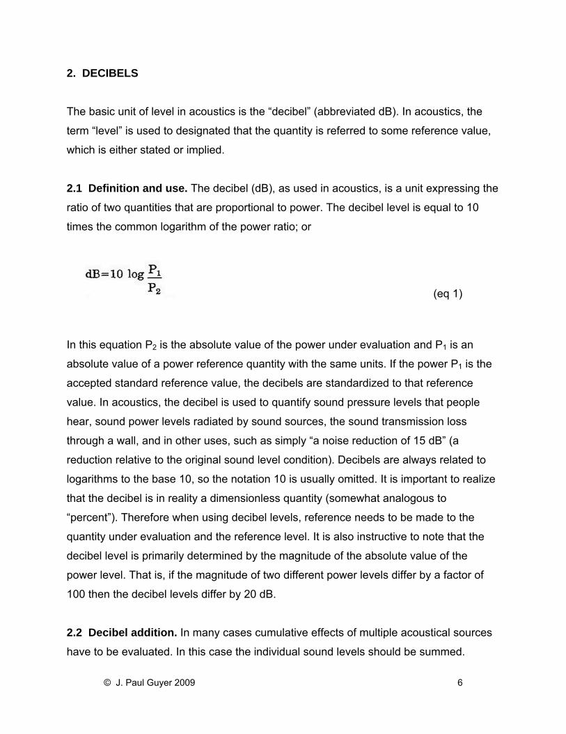
2.1 Definition and use. The decibel (dB), as used in acoustics, is a unit expressing the
ratio of two quantities that are proportional to power. The decibel level is equal to 10
times the common logarithm of the power ratio; or
(eq 1)
In this equation P2 is the absolute value of the power under evaluation and P1 is an
absolute value of a power reference quantity with the same units. If the power P1 is the
accepted standard reference value, the decibels are standardized to that reference
value. In acoustics, the decibel is used to quantify sound pressure levels that people
hear, sound power levels radiated by sound sources, the sound transmission loss
through a wall, and in other uses, such as simply “a noise reduction of 15 dB” (a
reduction relative to the original sound level condition). Decibels are always related to
logarithms to the base 10, so the notation 10 is usually omitted. It is important to realize
that the decibel is in reality a dimensionless quantity (somewhat analogous to
“percent”). Therefore when using decibel levels, reference needs to be made to the
quantity under evaluation and the reference level. It is also instructive to note that the
decibel level is primarily determined by the magnitude of the absolute value of the
power level. That is, if the magnitude of two different power levels differ by a factor of
100 then the decibel levels differ by 20 dB.
2.2 Decibel addition. In many cases cumulative effects of multiple acoustical sources
have to be evaluated. In this case the individual sound levels should be summed.
© J. Paul Guyer 2009 6
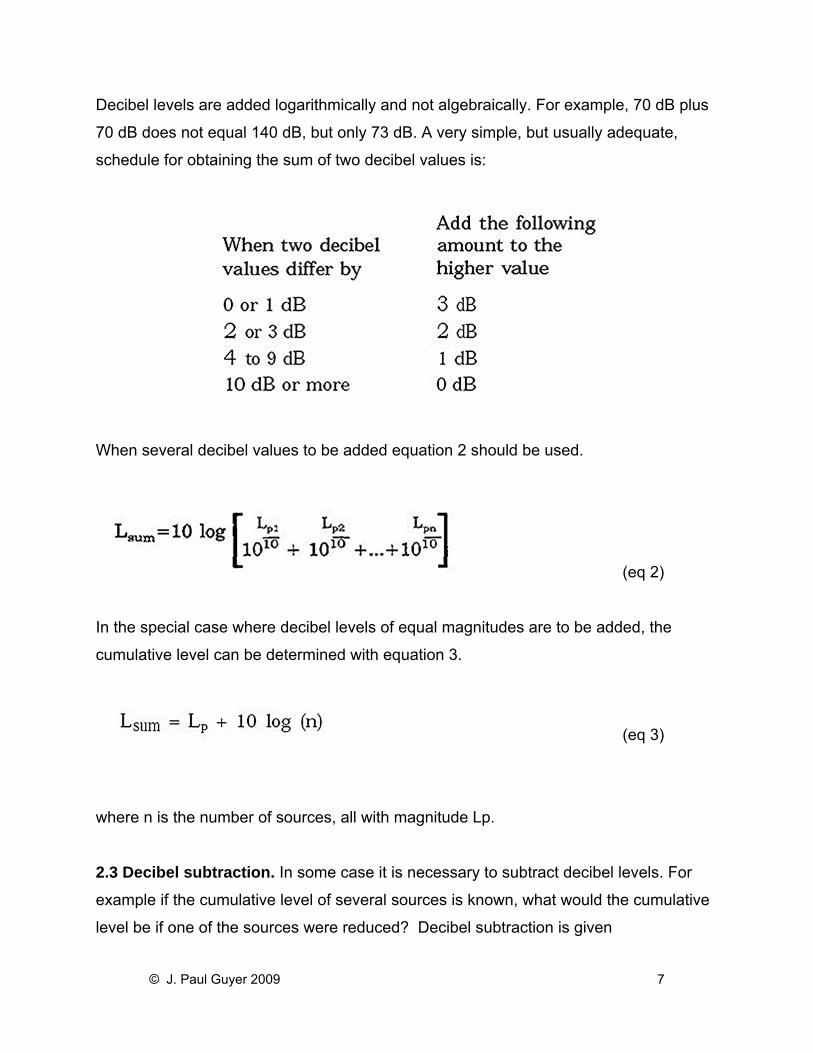
Decibel levels are added logarithmically and not algebraically. For example, 70 dB plus
70 dB does not equal 140 dB, but only 73 dB. A very simple, but usually adequate,
schedule for obtaining the sum of two decibel values is:
When several decibel values to be added equation 2 should be used.
(eq 2)
In the special case where decibel levels of equal magnitudes are to be added, the
cumulative level can be determined with equation 3.
(eq 3)
where n is the number of sources, all with magnitude Lp.
2.3 Decibel subtraction. In some case it is necessary to subtract decibel levels. For
example if the cumulative level of several sources is known, what would the cumulative
level be if one of the sources were reduced? Decibel subtraction is given
© J. Paul Guyer 2009 7
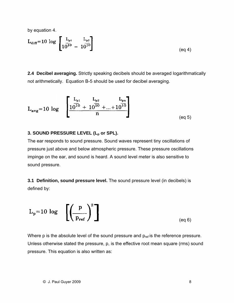
by equation 4.
(eq 4)
2.4 Decibel averaging. Strictly speaking decibels should be averaged logarithmatically
not arithmetically. Equation B-5 should be used for decibel averaging.
(eq 5)
3. SOUND PRESSURE LEVEL (Lp or SPL). The ear responds to sound pressure. Sound waves represent tiny oscillations of
pressure just above and below atmospheric pressure. These pressure oscillations
impinge on the ear, and sound is heard. A sound level meter is also sensitive to
sound pressure.
3.1 Definition, sound pressure level. The sound pressure level (in decibels) is
defined by:
(eq 6)
Where p is the absolute level of the sound pressure and pref is the reference pressure.
Unless otherwise stated the pressure, p, is the effective root mean square (rms) sound
pressure. This equation is also written as:
© J. Paul Guyer 2009 8
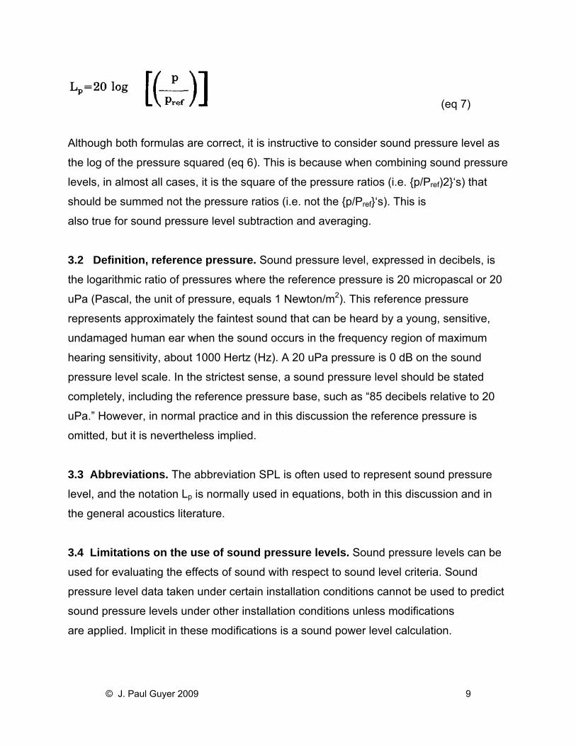
(eq 7)
Although both formulas are correct, it is instructive to consider sound pressure level as
the log of the pressure squared (eq 6). This is because when combining sound pressure
levels, in almost all cases, it is the square of the pressure ratios (i.e. {p/Pref)2}‘s) that
should be summed not the pressure ratios (i.e. not the {p/Pref}‘s). This is
also true for sound pressure level subtraction and averaging.
3.2 Definition, reference pressure. Sound pressure level, expressed in decibels, is
the logarithmic ratio of pressures where the reference pressure is 20 micropascal or 20
uPa (Pascal, the unit of pressure, equals 1 Newton/m2). This reference pressure
represents approximately the faintest sound that can be heard by a young, sensitive,
undamaged human ear when the sound occurs in the frequency region of maximum
hearing sensitivity, about 1000 Hertz (Hz). A 20 uPa pressure is 0 dB on the sound
pressure level scale. In the strictest sense, a sound pressure level should be stated
completely, including the reference pressure base, such as “85 decibels relative to 20
uPa.” However, in normal practice and in this discussion the reference pressure is
omitted, but it is nevertheless implied.
3.3 Abbreviations. The abbreviation SPL is often used to represent sound pressure
level, and the notation Lp is normally used in equations, both in this discussion and in
the general acoustics literature.
3.4 Limitations on the use of sound pressure levels. Sound pressure levels can be
used for evaluating the effects of sound with respect to sound level criteria. Sound
pressure level data taken under certain installation conditions cannot be used to predict
sound pressure levels under other installation conditions unless modifications
are applied. Implicit in these modifications is a sound power level calculation.
© J. Paul Guyer 2009 9
4. SOUND POWER LEVEL (Lw or PWL) Sound power level is an absolute measure of the quantity of acoustical energy
produced by a sound source. Sound power is not audible like sound pressure. However
they are related (see section 6). It is the manner in which the sound power is radiated
and distributed that determines the sound pressure level at a specified location. The sound power level, when correctly determined, is an indication of the sound radiated by
the source and is independent of the room containing the source. The sound power
level data can be used to compare sound data submittals more accurately and to
estimate sound pressure levels for a variety of room conditions. Thus, there is technical
need for the generally higher quality sound power level data.
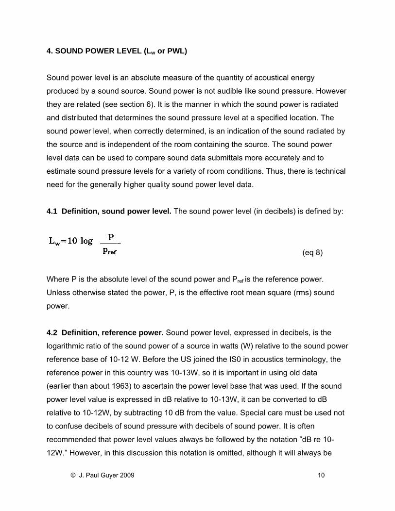
4.1 Definition, sound power level. The sound power level (in decibels) is defined by:
(eq 8)
Where P is the absolute level of the sound power and Pref is the reference power.
Unless otherwise stated the power, P, is the effective root mean square (rms) sound
power.
4.2 Definition, reference power. Sound power level, expressed in decibels, is the
logarithmic ratio of the sound power of a source in watts (W) relative to the sound power
reference base of 10-12 W. Before the US joined the IS0 in acoustics terminology, the
reference power in this country was 10-13W, so it is important in using old data
(earlier than about 1963) to ascertain the power level base that was used. If the sound
power level value is expressed in dB relative to 10-13W, it can be converted to dB
relative to 10-12W, by subtracting 10 dB from the value. Special care must be used not
to confuse decibels of sound pressure with decibels of sound power. It is often
recommended that power level values always be followed by the notation “dB re 10-
12W.” However, in this discussion this notation is omitted, although it will always be
© J. Paul Guyer 2009 10
made clear when sound power levels are used.
4.3 Abbreviations. The abbreviation PWL is often used to represent sound power
level, and the notation Lw normally used in equations involving power level. This custom
is followed in the manual.
4.4 Limitations of sound power level data. There are two notable limitations
regarding sound power level data: Sound power can not be measured directly but are
calculated from sound pressure level data, and the directivity characteristics of a source
are not necessarily determined when the sound power level data are obtained.
• PWL calculated, not measured. Under the first of these limitations, accurate
measurements and calculations are possible, but nevertheless there is no simple
measuring instrument that reads directly the sound power level value. The
procedures involve either comparative sound pressure level measurements
between a so-called standard sound source and the source under test (i.e. the
“substitution method”), or very careful acoustic qualifications of the test room in
which the sound pressure levels of the source are measured. Either of these
procedures can be involved and requires quality equipment and knowledgeable
personnel. However, when the measurements are carried out properly, the
resulting sound power level data generally are more reliable than most ordinary
sound pressure level data.
• Loss of directionality characteristics. Technically, the measurement of sound
power level takes into account the fact that different amounts of sound radiate in
different directions from the source, but when the measurements are made in a
reverberant or semi-reverberant room, the actual directionality pattern of the
radiated sound is not obtained. If directivity data are desired, measurements
must be made either outdoors, in a totally anechoic test room where reflected
sound cannot distort the sound radiation pattern, or in some instances by using
© J. Paul Guyer 2009 11
sound intensity measurement techniques. This restriction applies equally to both
sound pressure and sound power measurements.
5. SOUND INTENSITY LEVEL (Li) Sound intensity is sound power per unit area. Sound intensity, like sound power, is not
audible. It is the sound intensity that directly relates sound power to sound pressure.
Strictly speaking, sound intensity is the average flow of sound energy through a unit
area in a sound field. Sound intensity is also a vector quantity, that is, it has both a
magnitude and direction. Like sound power, sound intensity is not directly measurable,
but sound intensity can be obtained from sound pressure measurements.
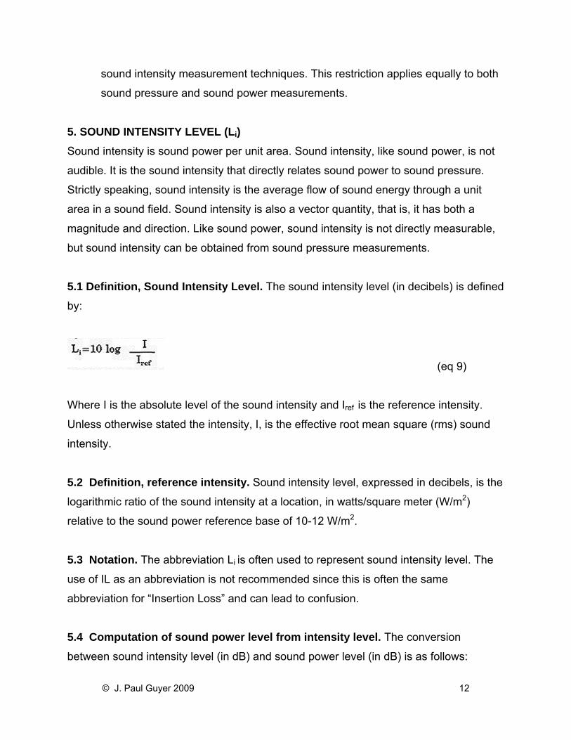
5.1 Definition, Sound Intensity Level. The sound intensity level (in decibels) is defined
by:
(eq 9)
Where I is the absolute level of the sound intensity and Iref is the reference intensity.
Unless otherwise stated the intensity, I, is the effective root mean square (rms) sound
intensity.
5.2 Definition, reference intensity. Sound intensity level, expressed in decibels, is the
logarithmic ratio of the sound intensity at a location, in watts/square meter (W/m2)
relative to the sound power reference base of 10-12 W/m2.
5.3 Notation. The abbreviation Li is often used to represent sound intensity level. The
use of IL as an abbreviation is not recommended since this is often the same
abbreviation for “Insertion Loss” and can lead to confusion.
5.4 Computation of sound power level from intensity level. The conversion
between sound intensity level (in dB) and sound power level (in dB) is as follows:
© J. Paul Guyer 2009 12

(eq 10)
where A is the area over which the average intensity is determined in square meter
(m2). Note this can also be written as:
LW = Li + 10 log{A} (eq 11)
if A is in English units (sq. ft.) then equation 11 can be written as:
LW = Li + 10 log{A} - 10 (eq 12)
Note, that if the area A completely closes the sound source, these equations can
provide the total sound power level of the source. However care must be taken to
ensure that the intensity used is representative of the total area. This can be done
by using an area weighted intensity or by logarithmically
combining individual Lw’s.
5.5 Determination of sound intensity. Although sound intensity cannot be measured
directly, a reasonable approximation can be made if the direction of the energy flow can
be determined. Under free field conditions where the energy flow direction is
predictable (outdoors for example) the magnitude of the sound pressure level (Lp) is
equivalent to the magnitude of the intensity level (Li). This results because, under these
conditions, the intensity (I) is directly proportional to the square of the sound pressure
(p2). This is the key to the relationship between sound pressure level and sound power
level. This is also the reason that when two sounds combine the resulting sound level is
proportional to the log of the sum of the squared pressures (i.e. the sum of the p2’s) not
the sum of the pressures (i.e. not the sum of the p’s). That is, when two sounds
combine it is the intensities that add, not the pressures. Recent advances in
measurement and computational techniques have resulted in equipment that
determines sound intensity directly, both magnitude and direction. Using this
© J. Paul Guyer 2009 13

instrumentation sound intensity measurements can be conducted in more complicated
environments, where fee field conditions do not exist and the relationship between
intensity and pressure is not as direct.
6. VIBRATION LEVELS Vibration levels are analogous to sound pressure levels.
6.1 Definition, vibration level. The vibration level (in decibels) is defined by:
(eq 13)
Where a is the absolute level of the vibration and aref is the reference vibration. In the
past different measures of the vibration amplitude have been utilized, these include,
peak-to-peak (p-p), peak (p), average and root mean square (rms) amplitude. Unless
otherwise stated the vibration amplitude, a, is the root mean square (rms). For simple
harmonic motion these amplitudes can be related by:
In addition vibration can be measured with three different quantities, these are,
acceleration, velocity and displacement. Unless otherwise stated the vibration levels
used in this manual are in terms of acceleration and are called “acceleration levels”. For
simple harmonic vibration at a single frequency the velocity and displacement can be
related to acceleration by:
© J. Paul Guyer 2009 14
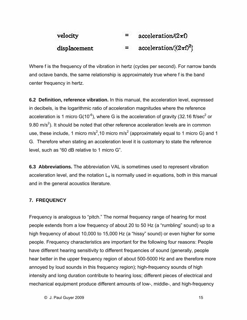
Where f is the frequency of the vibration in hertz (cycles per second). For narrow bands
and octave bands, the same relationship is approximately true where f is the band
center frequency in hertz.
6.2 Definition, reference vibration. In this manual, the acceleration level, expressed
in decibels, is the logarithmic ratio of acceleration magnitudes where the reference
acceleration is 1 micro G(10-6), where G is the acceleration of gravity (32.16 ft/sec2 or
9.80 m/s2). It should be noted that other reference acceleration levels are in common
use, these include, 1 micro m/s2,10 micro m/s2 (approximately equal to 1 micro G) and 1
G. Therefore when stating an acceleration level it is customary to state the reference
level, such as “60 dB relative to 1 micro G”.
6.3 Abbreviations. The abbreviation VAL is sometimes used to represent vibration
acceleration level, and the notation La is normally used in equations, both in this manual
and in the general acoustics literature.
7. FREQUENCY Frequency is analogous to “pitch.” The normal frequency range of hearing for most
people extends from a low frequency of about 20 to 50 Hz (a “rumbling” sound) up to a
high frequency of about 10,000 to 15,000 Hz (a “hissy” sound) or even higher for some
people. Frequency characteristics are important for the following four reasons: People
have different hearing sensitivity to different frequencies of sound (generally, people
hear better in the upper frequency region of about 500-5000 Hz and are therefore more
annoyed by loud sounds in this frequency region); high-frequency sounds of high
intensity and long duration contribute to hearing loss; different pieces of electrical and
mechanical equipment produce different amounts of low-, middle-, and high-frequency
© J. Paul Guyer 2009 15
noise; and noise control materials and treatments vary in their effectiveness as a
function of frequency (usually, low frequency noise is more difficult to control; most
treatments perform better at high frequency).
7.1 Frequency unit, hertz, Hz. When a piano string vibrates 400 times per second, its
frequency is 400 vibrations per second or 400 Hz. Before the US joined the IS0 in
standardization of many technical terms (about 1963), this unit was known as “cycles
per second.”
7.2 Discrete frequencies, tonal components. When an electrical or mechanical
device operates at a constant speed and has some repetitive mechanism that produces
a strong sound, that sound may be concentrated at the principal frequency of operation
of the device. Examples are: the blade passage frequency of a fan or propeller, the
gear-tooth contact frequency of a gear or timing belt, the whining frequencies of a
motor, the firing rate of an internal combustion engine, the impeller blade frequency of a
pump or compressor, and the hum of a transformer. These frequencies are designated
“discrete frequencies” or “pure tones” when the sounds are clearly tonal in character,
and their frequency is usually calculable. The principal frequency is known as the
“fundamental,” and most such sounds also contain many “harmonics” of the
fundamental. The harmonics are multiple of the fundamental frequency, i.e., 2, 3, 4, 5,
etc. times the fundamental. For example, in a gear train, where gear tooth contacts
occur at the rate of 200 per second, the fundamental frequency would be 200 Hz, and it
is very probable that the gear would also generate sounds at 400, 600, 800, 1000, 1200
Hz and so on for possibly 10 to 15 harmonics. Considerable sound energy is often
concentrated at these discrete frequencies, and these sounds are more noticeable and
sometimes more annoying because of their presence. Discrete frequencies can be
located and identified within a general background of broadband noise (noise that has
all frequencies present, such as the roar of a jet aircraft or the water noise in a cooling
tower or waterfall) with the use of narrowband filters that can be swept through the full
frequency range of interest.
© J. Paul Guyer 2009 16
7.3 Octave frequency bands. Typically, a piece of mechanical equipment, such as a
diesel engine, a fan, or a cooling tower, generates and radiates some noise over the
entire audible range of hearing. The amount and frequency distribution of the total noise
is determined by measuring it with an octave band analyzer, which is a set of
contiguous filters covering essentially the full frequency range of human hearing. Each
filter has a bandwidth of one octave, and nine such filters cover the range of interest for
most noise problems. The standard octave frequencies are given in table l. An octave
represents a frequency interval of a factor of two. The first column of table l gives the
band width frequencies and the second column gives the geometric mean frequencies
of the bands. The latter values are the frequencies that are used to label the various
octave bands. For example, the 1000-Hz octave band contains all the noise falling
between 707 Hz (1000/square root of 2) and 1414 Hz (1000 x square root of 2). The
frequency characteristics of these filters have been standardized by agreement (ANSI
S1.11 and ANSI S1.6). In some instances reference is made to “low”, “mid” and “high”
frequency sound. This distinction is somewhat arbitrary, but for the purposes of this
manual low frequency sound includes the 31 through 125 Hz octave bands, mid
frequency sound includes the 250 through 1,000 Hz octave bands, and high frequency
sound includes the 2,000 through 8,000 Hz octave band sound levels. For finer
resolution of data, narrower bandwidth filters are sometimes used; for example, finer
constant percentage bandwidth filters (e.g. half-octave, third-octave, and tenth-octave
filters), and constant width filters (e.g. 1 Hz, 10 Hz, etc.). The spectral information
presented in this manual in terms of full octave bands. This has been found to be a
sufficient resolution for most engineering considerations. Most laboratory test data is
obtained and presented in terms of 1/3 octave bands. A reasonably approximate
conversion from 1/3 to full octave bands can be made (see below). In certain cases the
octave band is referred to as a “full octave” or "1/1 octave” to differentiate it from partial
octaves such as the 1/3 or 1/2 octave bands. The term “overall” is used to designate the
total noise without any filtering.
7.4 Octave band levels (1/3). Each octave band can be further divided into three 1/3
octave bands. Laboratory data for sound pressure, sound power and sound intensity
© J. Paul Guyer 2009 17
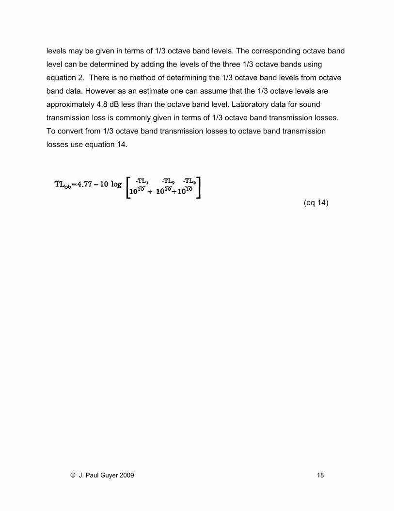
levels may be given in terms of 1/3 octave band levels. The corresponding octave band
level can be determined by adding the levels of the three 1/3 octave bands using
equation 2. There is no method of determining the 1/3 octave band levels from octave
band data. However as an estimate one can assume that the 1/3 octave levels are
approximately 4.8 dB less than the octave band level. Laboratory data for sound
transmission loss is commonly given in terms of 1/3 octave band transmission losses.
To convert from 1/3 octave band transmission losses to octave band transmission
losses use equation 14.
(eq 14)
© J. Paul Guyer 2009 18

Bandwidth and Geometric Mean Frequency of Standard Octave and 1/3 Octave Bands
Table 1
Where TLob is the resulting octave band transmission loss and TL1, TL2 & TL3 are the
1/3 octave band transmission losses.
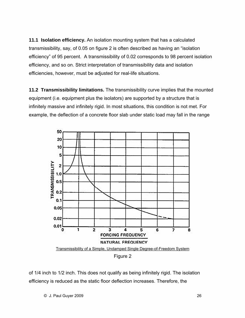
7.5 A-, B- & C-weighted sound levels. Sound level meters are usually equipped with
“weighting circuits” that tend to represent the frequency characteristics of the average
human ear for various sound intensities. The frequency characteristics of the A-, B-, and
C-weighting networks are shown in figure 2. The relative frequency response of the
average ear approximates the A curve when sound pressure levels of about 20 to 30 dB
are heard. For such quiet sounds, the ear has fairly poor sensitivity in the low-frequency
© J. Paul Guyer 2009 19
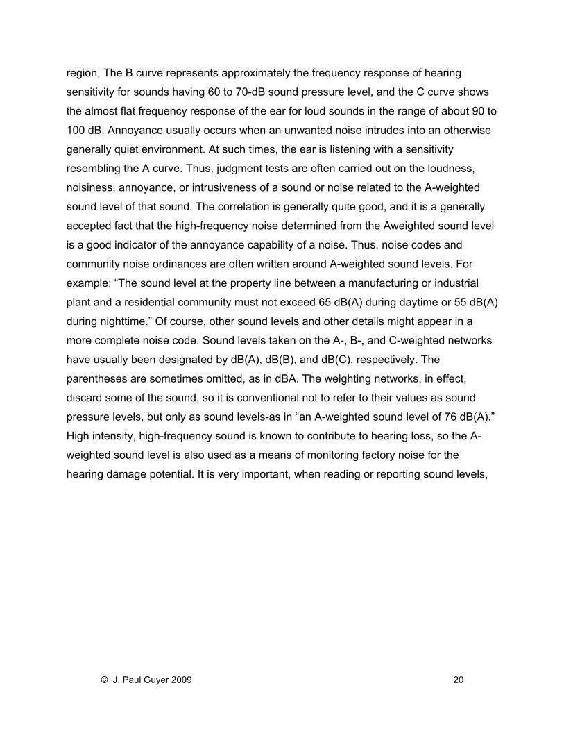
region, The B curve represents approximately the frequency response of hearing
sensitivity for sounds having 60 to 70-dB sound pressure level, and the C curve shows
the almost flat frequency response of the ear for loud sounds in the range of about 90 to
100 dB. Annoyance usually occurs when an unwanted noise intrudes into an otherwise
generally quiet environment. At such times, the ear is listening with a sensitivity
resembling the A curve. Thus, judgment tests are often carried out on the loudness,
noisiness, annoyance, or intrusiveness of a sound or noise related to the A-weighted
sound level of that sound. The correlation is generally quite good, and it is a generally
accepted fact that the high-frequency noise determined from the Aweighted sound level
is a good indicator of the annoyance capability of a noise. Thus, noise codes and
community noise ordinances are often written around A-weighted sound levels. For
example: “The sound level at the property line between a manufacturing or industrial
plant and a residential community must not exceed 65 dB(A) during daytime or 55 dB(A)
during nighttime.” Of course, other sound levels and other details might appear in a
more complete noise code. Sound levels taken on the A-, B-, and C-weighted networks
have usually been designated by dB(A), dB(B), and dB(C), respectively. The
parentheses are sometimes omitted, as in dBA. The weighting networks, in effect,
discard some of the sound, so it is conventional not to refer to their values as sound
pressure levels, but only as sound levels-as in “an A-weighted sound level of 76 dB(A).”
High intensity, high-frequency sound is known to contribute to hearing loss, so the A-
weighted sound level is also used as a means of monitoring factory noise for the
hearing damage potential. It is very important, when reading or reporting sound levels,
© J. Paul Guyer 2009 20
Approximate Electrical Frequency Response of
the A-, B-, and C-weighted Networks of Sound Level Meters.
Figure 2
to identify positively the weighting network used, as the sound levels can be quite
different depending on the frequency content of the noise measured. In some cases if
no weighting is specified, A-weighting will be assumed. This is very poor practice and
should be discouraged.
7.6 Calculation of A-weighted sound level. For analytical or diagnostic purposes,
octave band analyses of noise data are much more useful than sound levels from only
the weighting networks. It is always possible to calculate, with a reasonable degree of
accuracy, an A-weighted sound level from octave band levels. This is done by
subtracting the decibel weighting from the octave band levels and then summing the
levels logarithmically using equation 2. But it is not possible to determine accurately the
detailed frequency content of a noise from only the weighted sound levels. In some
instances it is considered advantageous to measure or report A-weighted octave band
levels. When this is done the octave band levels should not be presented as “sound
levels in dB(A)“, but must be labeled as “octave band sound levels with A-weighting”,
otherwise confusion will result.
© J. Paul Guyer 2009 21
8. TEMPORAL VARIATIONS Both the acoustical level and spectral content can vary with respect to time. This can be
accounted for in several ways. Sounds with short term variations can be measured
using the meter averaging characteristics of the standard sound level meter as defined
by ANSI S1.4. Typically two meter averaging characteristics are provided, these are
termed “Slow” with a time constant of approximately 1 second and “Fast” with a time
constant of approximately 1/8 second. The slow response is useful in estimating the
average value of most mechanical equipment noise. The fast response if useful in
evaluating the maximum level of sounds which vary widely.
9. SPEED OF SOUND AND WAVELENGTH The speed of sound in air is given by equation 15 where c is the speed of sound in air in
ft./set, and tF is the temperature in degrees Fahrenheit.
c = 49.03 x (460 + tF)1/2 (eq 15)
9.1 Temperature effect. For most normal conditions, the speed of sound in air can be
taken as approximately 1120 ft./sec. For an elevated temperature of about 1000 deg. F,
as in the hot exhaust of a gas turbine engine, the speed of sound will be approximately
1870 ft./sec. This higher speed becomes significant for engine muffler designs, as will
be noted in the following paragraph.
9.2 Wavelength. The wavelength of sound in air is given by equation 16.
Λ = c/f (eq 16)
Where Λ is the wavelength in ft., c is the speed of sound in air in ft./sec, and f is the
frequency of the sound in Hz. Over the frequency range of 50 Hz to 12,000 Hz, the
© J. Paul Guyer 2009 22

wavelength of sound in air at normal temperature varies from 22 feet to 1.1 inches, a
relatively large spread. The significance of this spread is that many acoustical materials
perform well when their dimensions are comparable to or larger than the wavelength of
sound. Thus, a l-inch thickness of acoustical ceiling tile applied directly to a wall is quite
effective in absorbing high-frequency sound, but is of little value in absorbing low
frequency sound. At room temperature, a l0-feet long dissipative muffler is about 9
wavelengths long for sound at 1000 Hz and is therefore quite effective, but is only about
0.4 wavelength long at 50 Hz and is therefore not very effective. At an elevated exhaust
temperature of 1000 deg. F, the wavelength of sound is about 2/3 greater than at room
temperature, so the length of a corresponding muffler should be about 2/3 longer in
order to be as effective as one at room temperature. In the design of noise control
treatments and the selection of noise control materials, the acoustical performance will
frequently be found to relate to the dimensions of the treatment compared to the
wavelengths of sound. This is the basic reason why it is generally easier and less
expensive to achieve high-frequency noise control (short wavelengths) and more
difficult and expensive to achieve low frequency noise control (long wavelengths).
B-10. LOUDNESS
The ear has a wide dynamic range. At the low end of the range, one can hear very faint
sounds of about 0 to 10 dB sound pressure level. At the upper end of the range, one
can hear with clarity and discrimination loud sounds of 100-dB sound pressure level,
whose actual sound pressures are 100,000 times greater than those of the faintest
sounds. People may hear even louder sounds, but in the interest of hearing
conservation, exposure to very loud sounds for significant periods of time should be
avoided. It is largely because of this very wide dynamic range that the logarithmic
decibel system is useful; it permits compression of large spreads in sound power and
pressure into a more practical and manageable numerical system. For example, a
commercial jet airliner produced 100,000,000,000 ( = 1011) times the sound power of a
cricket. In the decibel system, the sound power of the jet is 110 dB greater than that of
© J. Paul Guyer 2009 23
the cricket (110 = 10 log 1011). Humans judge subjective loudness on a still more
compressed scale.
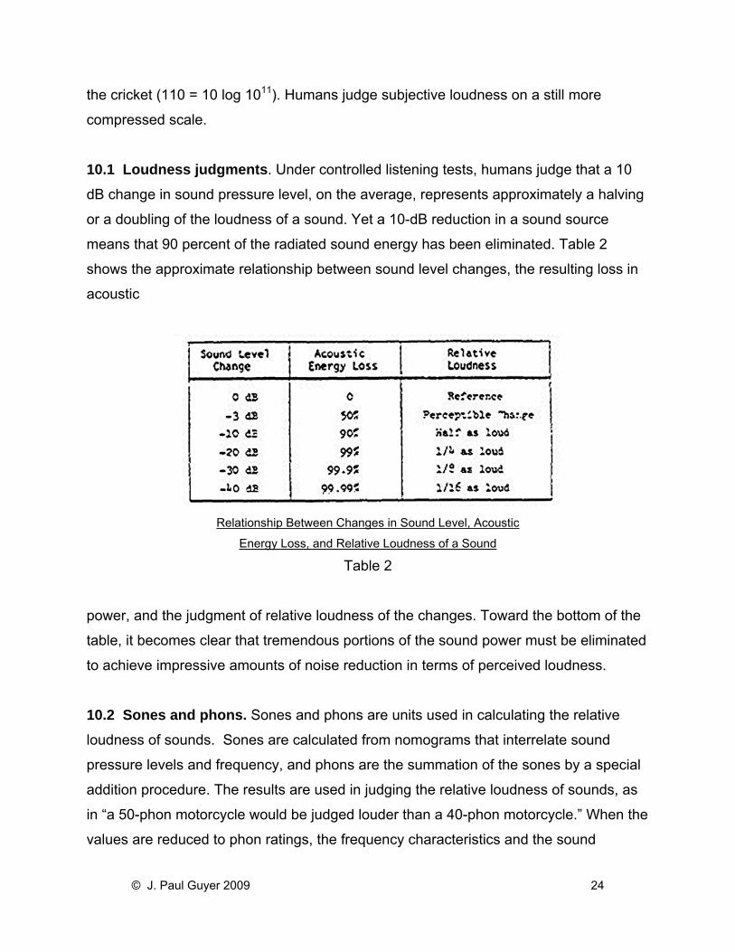
10.1 Loudness judgments. Under controlled listening tests, humans judge that a 10
dB change in sound pressure level, on the average, represents approximately a halving
or a doubling of the loudness of a sound. Yet a 10-dB reduction in a sound source
means that 90 percent of the radiated sound energy has been eliminated. Table 2
shows the approximate relationship between sound level changes, the resulting loss in
acoustic
Relationship Between Changes in Sound Level, Acoustic
Energy Loss, and Relative Loudness of a Sound
Table 2
power, and the judgment of relative loudness of the changes. Toward the bottom of the
table, it becomes clear that tremendous portions of the sound power must be eliminated
to achieve impressive amounts of noise reduction in terms of perceived loudness.
10.2 Sones and phons. Sones and phons are units used in calculating the relative
loudness of sounds. Sones are calculated from nomograms that interrelate sound
pressure levels and frequency, and phons are the summation of the sones by a special
addition procedure. The results are used in judging the relative loudness of sounds, as
in “a 50-phon motorcycle would be judged louder than a 40-phon motorcycle.” When the
values are reduced to phon ratings, the frequency characteristics and the sound
© J. Paul Guyer 2009 24
pressure level data have become detached, and the noise control analyst or engineer
has no concrete data for designing noise control treatments. Sones and phons are not
used in this discussion, and their use for noise control purposes is of little value. When
offered data in sones and phons, the noise control engineer should request the original
octave or 1/3 octave band sound pressure level data, from which the sones and phons
were calculated.
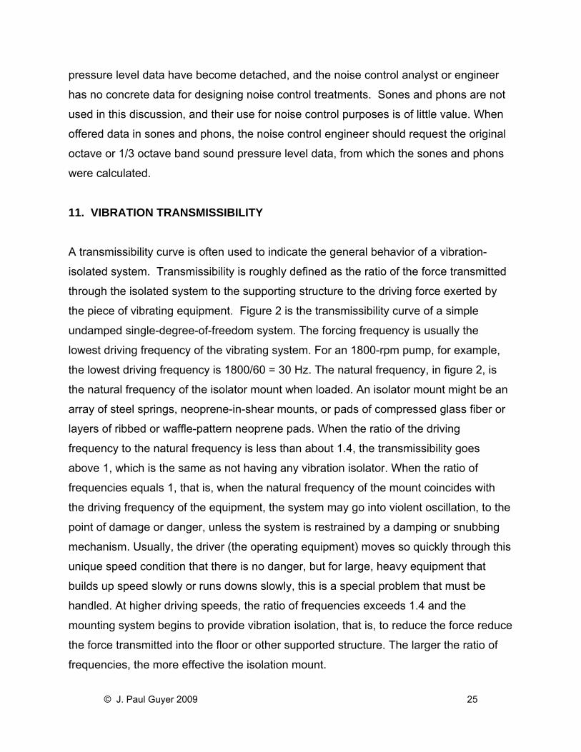
11. VIBRATION TRANSMISSIBILITY A transmissibility curve is often used to indicate the general behavior of a vibration-
isolated system. Transmissibility is roughly defined as the ratio of the force transmitted
through the isolated system to the supporting structure to the driving force exerted by
the piece of vibrating equipment. Figure 2 is the transmissibility curve of a simple
undamped single-degree-of-freedom system. The forcing frequency is usually the
lowest driving frequency of the vibrating system. For an 1800-rpm pump, for example,
the lowest driving frequency is 1800/60 = 30 Hz. The natural frequency, in figure 2, is
the natural frequency of the isolator mount when loaded. An isolator mount might be an
array of steel springs, neoprene-in-shear mounts, or pads of compressed glass fiber or
layers of ribbed or waffle-pattern neoprene pads. When the ratio of the driving
frequency to the natural frequency is less than about 1.4, the transmissibility goes
above 1, which is the same as not having any vibration isolator. When the ratio of
frequencies equals 1, that is, when the natural frequency of the mount coincides with
the driving frequency of the equipment, the system may go into violent oscillation, to the
point of damage or danger, unless the system is restrained by a damping or snubbing
mechanism. Usually, the driver (the operating equipment) moves so quickly through this
unique speed condition that there is no danger, but for large, heavy equipment that
builds up speed slowly or runs downs slowly, this is a special problem that must be
handled. At higher driving speeds, the ratio of frequencies exceeds 1.4 and the
mounting system begins to provide vibration isolation, that is, to reduce the force reduce
the force transmitted into the floor or other supported structure. The larger the ratio of
frequencies, the more effective the isolation mount.
© J. Paul Guyer 2009 25
11.1 Isolation efficiency. An isolation mounting system that has a calculated
transmissibility, say, of 0.05 on figure 2 is often described as having an “isolation
efficiency” of 95 percent. A transmissibility of 0.02 corresponds to 98 percent isolation
efficiency, and so on. Strict interpretation of transmissibility data and isolation
efficiencies, however, must be adjusted for real-life situations.
11.2 Transmissibility limitations. The transmissibility curve implies that the mounted
equipment (i.e. equipment plus the isolators) are supported by a structure that is
infinitely massive and infinitely rigid. In most situations, this condition is not met. For
example, the deflection of a concrete floor slab under static load may fall in the range
Transmissibility of a Simple, Undamped Single Degree-of-Freedom System
Figure 2
of 1/4 inch to 1/2 inch. This does not qualify as being infinitely rigid. The isolation
efficiency is reduced as the static floor deflection increases. Therefore, the
© J. Paul Guyer 2009 26
transmissibility values of figure 2 should not be expected for any specific ratio of driving
frequency to natural frequency.
• Adjustment for floor deflection. In effect, the natural frequency of the isolation
system must be made lower or the ratio of the two frequencies made higher to
compensate for the resilience of the floor. This fact is especially true for upper
floors of a building and is even applicable to floor slabs poured on grade (where
the earth under the slab acts as a spring). Only when equipment bases are
supported on large extensive portions of bedrock can the transmissibility curve
be applied directly.
• Adjustment for floor span. This interpretation of the transmissibility curve is
also applied to floor structures having different column spacings. Usually, floors
that have large column spacing, such as 50 to 60 feet, will have larger deflections
that floors of shorter column-spacing, such as 20 to 30 feet. To compensate, the
natural frequency of the mounting system is usually made lower as the floor span
increases. All of these factors are incorporated into the vibration isolation
recommendations in this chapter.
• Difficulty of field measurement. In field situations, the transmissibility of a
mounting system is not easy to measure and check against a specification. Yet
the concept of transmissibility is at the heart of vibration isolation and should not
be discarded because of the above weakness. The material that follows is based
on the valuable features of the transmissibility concept, but added to it are some
practical suggestions.
12. VIBRATION ISOLATION EFFECTIVENESS With the transmissibility curve as a guide, three steps are added to arrive at a fairly
practical approach toward estimating the expected effectiveness of an isolation mount.
© J. Paul Guyer 2009 27
12.1 Static deflection of a mounting system. The static deflection of a mount is
simply the difference between the free-standing height of the uncompressed, unloaded
isolator and the height of the compressed isolator under its static load. This difference is
easily measured in the field or estimated from the manufacturer’s catalog data. An
uncompressed 6 inch high steel spring that has a compressed height of only 4 inches
when installed under a fan or pump is said to have a static deflection of 2 inches. Static
deflection data are usually given in the catalogs of the isolator manufacturers or
distributors. The data may be given in the form of “stiffness” values. For example, a
stiffness of 400 lb/in. means that a 400 lb load will produce a 1 inch static deflection, or
that an 800 lb load will produce a 2 inch deflection, assuming that the mount has
freedom to deflect a full 2 inches.
12.2 Natural frequency of a mount. The natural frequency of steel springs and most
other vibration isolation materials can be calculated approximately from the formula in
equation 17.
(eq 17)
where fn is the natural frequency in Hz and SD is the static deflection of the mount in
inches.
• Example, steel spring. Suppose a steel spring has a static deflection of 1 inch
when placed under one corner of a motor-pump base. The natural frequency of
the mount is approximately:
• Example, rubber pad. Suppose a layer of 3/8-inch-thick ribbed neoprene is
used to vibration isolate high-frequency structure borne noise or vibration. Under
© J. Paul Guyer 2009 28
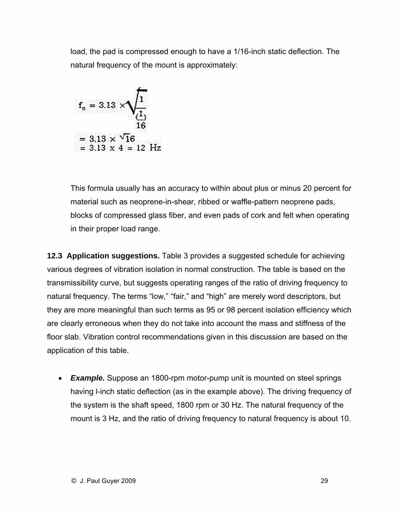
load, the pad is compressed enough to have a 1/16-inch static deflection. The
natural frequency of the mount is approximately:
This formula usually has an accuracy to within about plus or minus 20 percent for
material such as neoprene-in-shear, ribbed or waffle-pattern neoprene pads,
blocks of compressed glass fiber, and even pads of cork and felt when operating
in their proper load range.
12.3 Application suggestions. Table 3 provides a suggested schedule for achieving
various degrees of vibration isolation in normal construction. The table is based on the
transmissibility curve, but suggests operating ranges of the ratio of driving frequency to
natural frequency. The terms “low,” “fair,” and “high” are merely word descriptors, but
they are more meaningful than such terms as 95 or 98 percent isolation efficiency which
are clearly erroneous when they do not take into account the mass and stiffness of the
floor slab. Vibration control recommendations given in this discussion are based on the
application of this table.
• Example. Suppose an 1800-rpm motor-pump unit is mounted on steel springs
having l-inch static deflection (as in the example above). The driving frequency of
the system is the shaft speed, 1800 rpm or 30 Hz. The natural frequency of the
mount is 3 Hz, and the ratio of driving frequency to natural frequency is about 10.
© J. Paul Guyer 2009 29

Suggested Schedule for Estimating Relative Vibration Isolation Effectiveness of a Mounting System
Table 3
Table 3 shows that this would provide a “fair” to “high” degree of vibration isolation of
the motor pump at 30 Hz. If the pump impeller has 10blades, for example, this driving
frequency would be 300 Hz, and the ratio of driving to natural frequencies would be
about 100; so the isolator would clearly give a “high” degree of vibration isolation for
impeller blade frequency.
• (2) Caution. The suggestion on vibration isolation offered in this discussion are
based on experiences with satisfactory installations of conventional electrical and
mechanical HVAC equipment in buildings. The concepts and recommendations
described here may not be suitable for complex machinery, with unusual
vibration modes, mounted on complex isolation systems. For such problems,
assistance should be sought from a vibration specialist.
© J. Paul Guyer 2009 30
Top Related