


Languages
Pages
Legal

Annals ofGlaciology 27 1998 © International Glaciological Society
Cotnparison of ERS satellite radar altitneter heights with GPS-derived heights on the Amery Ice Shelf, East Antarctica
HELEN A. PHILLIPS/ IAN ALLISON,2 R. COLE MAN,3 G. HYLAND,2 PETER]' MORGA ,4 N.W. YOU NG2
IAntarctic GRG and lA SOS, University of Tasmania, Box 252-80, Hobart, Tasmania 700}, Australia 2Antarctic eRe and Australian Antarctic Division, Box 252-80, Hobart, Tasmania 7001, Australia
3 Antarctic eRe and Department rif Geography and Environmental Studies, University oJTasmania, Box 252-80, Hobart, Tasmania 7001, Austral£a
4 Faculty of Info rmation Sciences and Engineering, University qfGanbena, Box }, BeLconnen, Australian Capital Ten ito1Y 2616, Australia
ABSTR ACT. In the spring of 1995 an extensive global positioning system (GPS) survey was carried out on the Amery Ice Shelf, East Antarctica, providing ground-truth ell ipsoidal height measurements for the European remote-sensing satellite (ERS) : adar altimeters. GPS- and altimeter-derived surface heights have been compared at the 111tersecting points of the ERS ground tracks and the GPS survey. The mean a nd rms height difference for all ERS-I geodetic-phase tracks across the survey region is 0.0 ± 0.1 m a nd 1.7 m, respec tively. The spatia l distribution of the height differences is highly correlated with surface topographic variations. Compari sons of GPS-derived surface-elevation profiles along ERS ground tracks show that the ERS a ltimeters can closely follow the GPS repre entation of the actual surface.
1. INTRODUCTION
The satellite radar altimeter is an invaluable instrument for providing height measurements over ice sheets and ice shelves. The periodic monitoring of the pola r regions using such measurements has long been proposed by the climatechange and glaciological communities (Robin, 1966). The first altimeter study on the Amery Ice Shelf, East Antarctica, was made by Brooks and others (1983) using Seas at da ta. They compared an altimeter-derived digital elevation model (DEM ) with levell ing data from a traverse made 9 years previously to look for evidence of elevation change over that period. A subsequent study looking for evidence of elevation changes in the Lambert Glacier- Amery Ice Shelf system employed orbit crossove r analysis of Seasat and Geosat altimeter data (Lingle and others, 1994).
The internal consistency of a ltimeter height measurements can be determined by comparing surface heights along repeating tracks, and at exact crossover locations (Brooks and others, 1978). However, in order to assess the quality of the absolute height measurement and to determine how well the altimeter height profile represents the true surface, an independently surveyed reference surface, referenced to the same ellipsoid and from the same epoch, is required. Such a surface can be obtained using kinematic global positioning system (GPS) surveying techniques. This paper presents the results of a GPS survey carried out on the Amery Ice Shelf during the austral spring of 1995, designed to provide a height reference surface for the European remote-sensing satell ite (ERS-I and ERS-2) altimeters.
2. GPS FIELD SURVEY AND DATA PROCESSING
The field programme took place on the Amery Ice Shelf
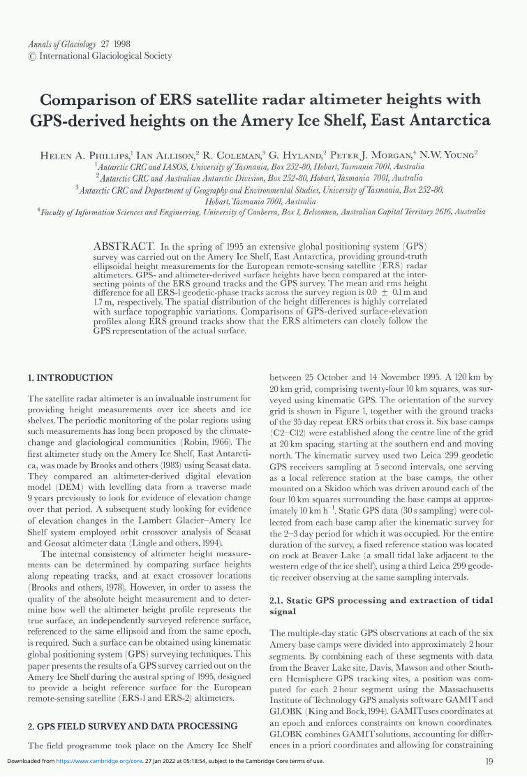
between 25 O ctober and 14 November 1995. A 120 km by 20 km grid, comprising twenty-four 10 km squares, was surveyed using kinematic GPS. The ori enta tion of the survey grid is shown in Figure I, together with the ground tracks of the 35 day repeat ERS orbits th at cross it. Six base camps (C2- C I2) were established along the centre line of the grid at 20 km spacing, starting a t the southern end and moving north . The kinematic survey used two Leica 299 geodetic GPS receivers sampling at 5 second intervals, one serving as a local reference station a t the base camps, the other mounted on a Skidoo which was driven a round each of the four 10 km squares surrounding the base camps at approximately 10 km h - I. Static GPS data (30 s sampling) were collected from each base camp after the kinematic survey for the 2- 3 day period for which it was occupied. For the entire duration of the survey, a fi xed reference sta tion was located on rock at Beaver Lake (a small tidal lake adjacent to the western edge of the ice shelf), using a third Leica 299 geodetic receiver observing at the same sampling intervals.
2.1. Sta t ic GPS processing and extraction of tidal signal
The multiple-day sta tic GPS observations at each of the six Amery base camps were divided into approximately 2 hour segments. By combining each of these segments with data from the Beaver Lake site, Davis, Mawson and other Southern H emisphere GPS tracking sites, a position was compu ted for each 2 hour segment using the Massachuse tts Institute of Technology GPS a nalysis softwa re GAMIT and GLOBK (King and Bock, 1994). GAMITuses coordinates at an epoch and enforces constraints on known coordinates. GLOBK combines GAMITsolutions, accounting for differences in a priori coordinates and allowing for constraining
19 Downloaded from https://www.cambridge.org/core. 27 Jan 2022 at 05:18:54, subject to the Cambridge Core terms of use.
Phillips and others: Comparison of altimeter- and GPS-derived heights on Amery Ice Shelf
., " "-""'.- -
Fig. 1. Location of survey grid and ERS altimeter ground tracks on the Amery lee Shelf. The survey grid dimensions are 120 km x 20 km (adjacent grid nodes are 10 km apart). Base camps (C2- C12) were established at every second grid node along the centre line, and at Beaver Lake. Arrows on ERS tracks indicate the direction ofsatellite travel. Areas of no shading denote the approximate extent qf the ice shelf; light shading denotes grounded ice; and the darkest shading indicates open or ice-covered water.
velocities to an a priori model. The 2 hourly averaged positions were calculated using a precise 3 day orbit for each camp, which overcame the discontinuities associated with short-span data in 24 hour segments. The movement was transformed into horizontal and vertical components tangential and normal to the surface of the World Geodetic System 1984 (WGS84) ellipsoid, which closely represent surface ice flow and vertical height variations, respectively.
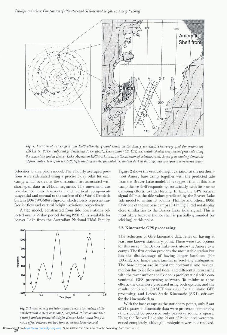
A tide model, constructed from tide observations collected over a 22 day period during 1990- 91, is available for Beaver Lake from the Australian National Tidal Facility.
1200
• 1000
800
E600 S-E
f 400
20
200
0
- 200 0 0.5
• 1.5
lime (days) 2 2.5
Fig. 2. Time series qf the tide-induced vertical variation at the northernmost Ame1Y base camp, computed at 2hour intervals (stars), and the predicted tideJor Beaver Lake (solid line). A mean iffset between the two time series has been removed.
Figure 2 shows the vertical-height variation at the northernmost Amery base camp, together with the predicted tide from the Beaver Lake model. This suggests that at this base camp the ice shelf responds hydrostatically, with little or no damping effects, to tidal forcing. In fact, the GPS vertical signal follows the tide values predicted by the Beaver Lake tide model to within 10- 50 mm (Phillips and others, 1996). Only one of the six base camps (C4 in Fig. I) did not display close similarities to the Beaver Lake tidal signaL This is most likely because the ice shelf is partially grounded (or sticking) at this point.
2.2. K in ell1.atic GPS processin g
The reduction of GPS kinematic data relies on having at least one known stationary point. There were two options for this survey: the Beaver Lake rock site or the Amery base camps. The first option provides the most stable station but has the disadvantage of having longer baselines (60-100 km), and hence uncertainties in resolving ambiguities. The base camps are in constant horizontal and vertical motion due to ice flow and tides, and differential processing with the rover unit on the Skidoo is problematical with conventional GPS processing software. To minimise these effects, the data were processed using both options, and the results combined. GAMIT was used for the static GPS processing, and Leica's Static Kinematic (SKI ) software for the kinematic data.
With the base camps as the stationary points, only 2 out of 24 squares of kinematic data were processed completely; others could be processed only part-way round a square. Using the Beaver Lake site, 21 out of 24 squares were processed completely, although ambiguities were not resolved.
Downloaded from https://www.cambridge.org/core. 27 Jan 2022 at 05:18:54, subject to the Cambridge Core terms of use.
Phillips and others: Comparison qf altimeter- and GPS -derived heights on Amery !ce Shelj
The GPS closure, i.e. the rms differences in the base-camp station coordinates between the start and finish of the sur
vey, was approx imately 0.4 m in a ll three components (lati
tude, longitude and height).
3. ALTIMETER DATA PROCESSING
The ERS altimeters have been operated with different orbi
tal repeat periods: 3, 35 and 168 days. In this analysis we have used data from both the 35 day phase (October and November 1995) and the 168 day geodetic phase (April 1994- March 1995).
By using the 35 day data from the same time period as the field survey, we hope to have minimised any temporal height bias due to seasonal variations in penetration depth of the radar signal, resulting from changes in surface properties of the ice shelf (Ridley and Partington, 1988). Figure I shows the five ERS satellite ground tracks from the 35 day phase that cross the GPS survey grid. There are two repeat cycles of ERS-2 and one cycle of ERS-I available from October and November 1995, all in ice mode.
The 168 day data provide a m uch denser spatial coverage over the survey region: 2- 3 km between adj acent ground tracks, compared to approximately 30 km between adjacent tracks for the 35 day data. There are 48 ER S-I satellite tracks from the geodetic phase that cross the GPS survey grid, all in ice mode.
There are a number of known biases and errors inherent in surface heights inferred from altimeter range measurements coll ected over an ice sheet or ice shelf. Those that have been corrected for in this analysis are listed below.
3.1. Merging of precise orbits
Highly precise orbits (relative to the WGS84 ellipsoid ) produced with the Delft Gravity Model DGM-E04, based on satelli te laser ranging, a ltimeter residuals and altimeter crossovers, were recently made available by the Delft Un iversity of Technology (Scharoo and others, in press). These orbits were used to update the spacecraft position. The radial precision of the Delft orbits is approximately 90 mm.
3.2. Retracking
The power received from each return altimeter echo is recorded as a waveform within a finite-width range window, quantised into 64 range bins of equal width (1.82 m in ice mode), with the leading edge corresponding to the initial interaction with the surface. The range measurement is made to the midpoint of the range window, and therefore, to obtain the true range, the distance to the leading edge needs to be determined. The technique used to do this is the simple offset centre of gravity (OCOG ) algorithm, descr ibed by Wi ngham and others (1986). A percentage threshold value, determined by the total power under the waveform, is used to locate the retrack point on the leading edge. Retracking corrections in this analysis were made using the 10% , 25% and 50% threshold values.
3.3. Tidal correction
The ocean-tide values supplied in the altimeter records were derived from a model that is not valid over ice shelves. As previously mentioned, the GPS vertical height variation observed over the ice-shelf survey region closely matches
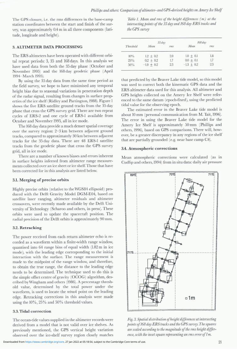
Table 1. Mean and rms cif the height dijfirences (m) at the intersecting points qf the 35 day and 168 day ERS tracks and the GPS survey
35 day 168 day Threshold AIieall rms j\!Jean 1"1ns
10% 1.2 ± 0.2 2.0 1.0 ± 0.1 1.8 25% 0.2 ± 0.2 1.7 0.0 ± 0.1 1.7 50% - 1.0 ± 0.2 2.3 - 1.3 ± 0.2 2.3
that predicted by the Beaver Lake tide model, so this model was used to correct both the kinematic GPS data and the ERS altimeter data used for this analysis. All a ltimeter and GPS heights collected on the Amery Ice Shelf were referenced to the same datum (epoch-fixed ), using the predicted tidal value for the observing epoch.
The estimated error in the Beaver Lake tide model is about 10 mm (personal communication from M. Tait, 1996). The error in using the Beaver Lake tide model for the Amery Ice Shelf is approximately 50 mm (Phillips and others, 1996), based on GPS comparisons. There wi ll , however, be a greater discrepancy in any regions of the ice shelf that are partially grounded (e.g. near base camp C4).
3.4. Atmospheric corrections
Mean atmospheric corrections were calculated (as in Cudlip and others, 1994) from in situ data: daily air pressure
69'1:; 70'1:; 71 'E:
7.t'S .. ~ .. ... . . .. · .
o1m
Fig. 3. Spatial distribution cifheight dijfirences at intersecting points qf 168 day ERS tracks and the GPS survey. The squares are scaled according to the magnitude qf the rms height difference' with the inset square representing an rms error qf 1 m.
21 Downloaded from https://www.cambridge.org/core. 27 Jan 2022 at 05:18:54, subject to the Cambridge Core terms of use.
Phillips and others: Comparison if altimeter- and GPS -derived heights on Amery Ice Shelf
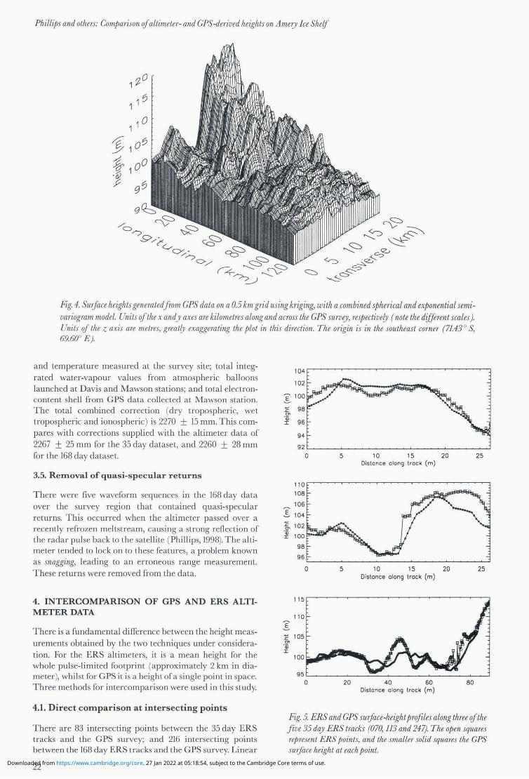
Fig. 4. Surface heights generated from GPS data on a 0.5 km grid using kriging, with a combined spherical and exponential semivariogram model. Units of the x and y axes are kilometres along and across the GPS survey, respectively (note the dijJerent scales). Units if the z axis are metres, greatly exaggerating the plot in this direction. The origin is in the southeast corner (7l.43 0 S, 69.600 E).
and temperature measured at the survey site; total integrated water-vapour values from atmospheric balloons launched at Davis and Mawson stations; and total electroncontent shell from GPS data collected at Mawson station. The total combined correction (dry tropospheric, wet tropospheric and ionospheric ) is 2270 ± 15 mm. This compares with corrections supplied with the altimeter data of 2267 ± 25 mm for the 35 day dataset, and 2260 ± 28 mm for the 168 day dataset.
3.5. Retnoval of quasi-specular returns
There were five waveform sequences in the 168 day data over the survey region that contained quasi-specular returns. This occurred when the altimeter passed over a recently refrozen meltstream, causing a strong reflection of the radar pulse back to the satellite (Phillips, 1998). The altimeter tended to lock on to these features , a problem known as snagging, leading to an erroneous range measurement. These returns were removed from the data.
4. INTERCOMPARISON OF GPS AND ERS ALTIMETER DATA
There is a fundamental difference between the height measurements obtained by the two techniques under consideration, For the ERS altimeters, it is a mean height for the whole pulse-limited footprint (approximately 2 km in diameter), whilst for GPS it is a height ofa single point in space, Three methods for intercomparison were used in this study,
4.1. Direct cotnparison at intersecting points
104
I :E 0'
'0; 96 I
94
92 0
110
106
I 104
:g, 102 '0;
100 I
98
96
0
115
110
I :E 105 0'
'0; I
95 0
5 10 15 20 Distance along track (m)
5 10 15 20 Distance along track (m)
20 40 60 80 Distance along track (m)
25
25
There are 83 intersecting points between the 35 day ERS tracks and the GPS survey; and 216 intersecting points between the 168 day ERS tracks and the GPS survey, Linear
Fig. 5. ERS and GPS surface-height prrifiles along three of the five 35 dr.ry ERS tracks (070, 113 and 247), The open squares represent ERS points, and the smaller solid squares the GPS surface height at each point.
22 Downloaded from https://www.cambridge.org/core. 27 Jan 2022 at 05:18:54, subject to the Cambridge Core terms of use.
Phillips and others: Comparison if altimeter- and GPS -derived heights on Amery Ice Shelf
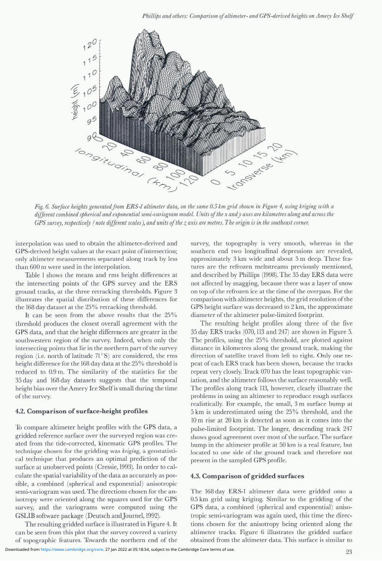
Fig. 6. Surface heights generatedfrom ERS-I altimeter data, on the same 0.5 km grid shown in Figure 4, using kriging with a different combined spherical and exponential semi-variogram model. Units rif the x and y axes are kilometres along and across the GPS SUrVlry, respectively (note different scales), and units rif the z axis are metres. The origin is in the southeast corner.
interpolation was used to obtain the altimeter-derived and GPS-derived height values at the exact point of intersection; only a ltimeter measurements separated a long track by less than 600 m were used in the interpolation.
Table I shows the means and rms height differences at the intersecting points of the GPS survey and the ERS ground tracks, at the three retracking thresholds. Figure 3 illustrates the spatial distribution of these differences for the 168 day dataset at the 25% retracking threshold.
It can be seen from the above results that the 25% threshold produces the closest overall agreement with the GPS data, and that the height differences a re greater in the southwestern region of the survey. Indeed, when only the intersecting points that lie in the northern part of the survey region (i. e. north of latitude 71°S) are considered, the rms height difference for the 168 day data at the 25% threshold is reduced to 0.9 m. The similarity of the statistics for the 35 day and 168 day datasets suggests that the temporal height bias over the Amery Ice Shelfis small during the time of the su rvey.
4.2. Comparison of surface-height profiles
To compare altimeter height profiles with the GPS data, a gridded reference surface over the surveyed region was created from the tide-corrected, kinematic GPS profiles. The technique chosen for the gridding was kriging, a geosta tistical technique that produces an optimal prediction of the surface at unobserved points (Cressie, 1993). In order to calculate the spatial variability of the data as accurately as possible, a combined (spherical and exponential) anisotropic semi-variogram was used. The directions chosen for the anisotropy were oriented along the squares used for the GPS survey, and the variograms were computed using the GSLIB software package (Deutsch andJournel, 1992).
The resulting gridded surface is illustrated in Figure 4. It can be seen from this plot that the survey covered a variety of topographic features. Towards the northern end of the
survey, the topography is very smooth, whereas in the southern end two longitudinal depressions are revealed, approximately 3 km wide and about 5 m deep. These features are the re frozen meltstreams previously mentioned, and described by Phillips (1998). The 35 day ERS data were not affected by snagging, because there was a layer of snow on top of the refrozen ice at the time of the overpass. For the compari son with altimeter heights, the grid resolu tion of the GPS height surface was decreased to 2 km, the approximate diameter of the a ltimeter pulse-limited footprint.
The resulting height profi les along three of the five 35 day ERS tracks (070, 113 and 247) are shown in Figure 5. The profiles, using the 25% threshold, are plotted against distance in kilometres a long the ground track, making the direction of satellite travel from left to right. Only one repeat of each ERS track has been shown, because the tracks repeat very closely. Track 070 has the least topographic variation, and the altimeter follows the surface reasonably well. The profil es along track 113, however, clearly illustrate the problems in using an altimeter to reproduce rough surfaces reali stically. For example, the small, 3 m surface bump at 5 km is underestimated using the 25% threshold, and the 10 m rise at 20 km is detected as soon as it comes into the pulse-limited footprint. The longer, descending track 247 shows good agreement over most of the surface. The surface bump in the altimeter profile at 50 km is a real feature, but located to one side of the ground track and therefore not present in the sampled GPS profile.
4.3. Comparison of gridded surfaces
The 168 day ERS-I a ltimeter data were gridded onto a 0.5 km grid using kriging. Simi la r to the gridding of the GPS data, a combined (spherical and exponential) anisotropic semi-variogram was again used, this time the directions chosen for the anisotropy being oriented along the altimeter tracks. Figure 6 illustrates the gridded surface obtained from the altimeter data. This surface is similar to
23 Downloaded from https://www.cambridge.org/core. 27 Jan 2022 at 05:18:54, subject to the Cambridge Core terms of use.
Phillips and others: Comparison if altimeter -and GPS -derived heights on Ame1Y Ice Shelf
that generated from the GPS data (Fig. 4), but the altimeter surface is smoother and most of the features appear broader. T his is to be expected, because the altimeter measures a mean surface height over the area of the pulse-limited footprint, and a lso tends to "see" high features early, as seen in
track 113 (Fig. 5).
5. CONTRIBUTIONS TO OBSERVED HEIGHT DIFFERENCES
Differences between the ERS altimeter-derived heights and the GPS-derived heights can arise from a number of possible sources. The combined rms error remaining in the altimeter height measurements after merging in the precise orbits (rvgO mm ) and correcting for propagation delays (-"-'15mm) and tidal motion (",50 mm) is ",104 mm. The
rms error introduced by the OCOG re tracking method is
0.49 m per waveform in ice mode (Scott and others, 1994), which amounts to ",80 mm for the 35 day dataset (83 intersections ), and ",50 mm for the 168 day dataset (216 intersections). The potential remaining sources of bias are:
Terrain bias: the shape of the altimeter waveform re
ceived by a radar altimeter is dependent on the properties of the surface with which the pulse interacts, and will be distorted to a varying degree, depending on inhomogeneities on the surface. No simple retracker can account for these non-uniform waveforms, and techniques such
as waveform migration (Wingham and others, 1993) are
being developed to cope with this problem.
Suiface layer penetration: this problem has been approached by Davis (1993) in his surface and volume retracking program, but has not been fu lly tested [or ice mode, where there is a wider range window and the
waveforms are more coarsely sampled. Surface penetration is of the order of I m on the Amery Ice Shelf, wh ich introduces a height bias of about 10 cm (personal comm unication from]. Rid ley, 1997).
6. CONCLUSIONS
It has been shown that the ERS altimeters can reproduce the surface topography o[ an ice shelf, closely matching that obtained through ground survey, especially when the surface topography is smooth. At the 25 % threshold in the OCO G a lgorithm, the mean and rms height differences at the intersecting points of the ER S-l geodetic phase tracks with the GPS survey are 0.0 ± 0.1 m and 1.7 m, respectively. The spatial d istribution of the height differences is highly correlated with the topographic variations evident in the g ridded surface.
The total rms error remaining in the ERS altimeter
height measurements, after merging in the precise orbits and correcting for propagation delays, tidal motion and tracking error, is at most 0.13 m. This error, combined with the GPS closure error of 0.4 m, does not fu ll y account for the rms height difference of 1.7 m between the ERS and GPS heights. The only remaining sources of discrepancy are
biases in the ER S heights arising from terrain effects and, to a lesser extent, surface layer penetration. An a priori knowledge of the surface topography would be required to extract more accurate height information from satell ite altimetry over ice regions.
24
This study has provided an accurate ground-truthing reference surface for the ERS a ltimeters, due to the large survey area and the high precision of the GPS coordinates. Data from the geodetic phase ofERS-1 are being used within the Antarctic CRC to generate a high-resolution, accurate DEM of the Amery Ice Shelf. The reference surface will also be used, in conjunction with height measurements from future altimeter missions, to provide ongoing monitoring of elevation change on the Amery Ice Shelf.
ACKNOWLEDGEMENTS
The authors would like to thank: the Amery team members for the fieldwork (M. Craven, R. M anson, A. Ruddell, P. J ohnson, S. Anglesey and P. Scholtz); the Australian National Tidal Facility at Flinders University, South Australia,
for Beaver Lake tidal predictions; M . Craven for producing Figure I; ]. Ridley and R. M assom for reviewing early versions of the manuscript; R. Manson for her role in processing the GPS data; and N. Adams for suppl ying atmospheric data. The ERS radar altimeter data are copy
right to the European Space Agency, 1991 - 96, and provided through AO project ERS.A02.AUS103.
REFERENCES
Brooks, R. L. , W.]. Campbcll, R. O. Ramseier, H . R. Stanlcy and H.]. Zwa lly. 1978. lee sheet topography by satellite a ltimetry. Nature, 274 (5671),539- 543.
Brooks, R. L. , R. S. Williams, Jr,J G. Ferrigno and W. B. Krabil l. 1983. Amery Ice Shclftopography from satel lite radar a ltimetry. III Oliver, R. L. , P. R. James and]. B. J ago, eds. Antarctic earth science. Cambridge, etc., Cambridge University Press, 441 - 445.
Cressic, N. A. C. 1993. Statisticsjor spatial data. New York, etc., J oh n Wi ley and Sons.
Cudlip, \V and 7 others. 1994. Corrections for a ltimeter low-l evel processing at the Earth Observation Data Centre. 1nl. ] Remote Sensing, 15(4),889- 914.
Davis, e. H. 1993. A surface and vo lume sca ttering retracking algorithm for ice shee t satellite altimetry. IEEE Trans. Ceosci. Remote Sensing, GE-31 (4), 811 - 818.
Deutsch, C. and A. J ournel. 1992. GSLIB geostatistical sqfiwarelibrary and user's guide. Oxrord, Oxrord University Press.
King, R. W. and Y. Bock. 1994. The MIT GPS anaD'sis sqfiware (GAMIT). Cambridge, MA, Massachusetts Institute of Technology.
Lingle, e. S. , L. Lee, H.]. Zwally and T.e. Seiss. 1994. Recent elevation increase o n Latnbert Glacier, Antarctica , frolll o rbit cross-over anal ys is of sat cl lite-radar altimetry. Ann. Clacio!. , 20, 26- 32.
Phillips, H . A. 1998. Surface meltstreams on the Amery Ice Shelf, East Antarctica. Ann. Glaciol., 27 (see paper en this vo lume).
Phillips, H. A. , I. Allison, M. Craven, K. Krebs and P Morgan. 1996. lee velocity, mass nux and grounding line location on the Lambert Glacier -Amery Ice Shclfsystcm. [Abstract.] EOS, 77 (22), Western Pacific Geophysics Meeting Supplement, WI3.
Ridl ey, J K. and K . e. Partington. 1988. A model of satellite radar a ltimeter return from ice shects. Int. ] Remote Sensing, 9 (4),601- 624.
Robin, G. de Q 1966. Mapping the Antarctic ice sheet by satellite altimetry. Can. J Earth Sci., 3(6), 893- 901.
Scharroo, R., P Visser and G. Mets. In press. Precise orbit detcrmination and gravity fi eld improvement for the ERS sa tellites. ] Ceophys. Res ..
SCOtl, R. F. and 11 others. 1994. A comparison of the performance of the ice and ocean tracking modes of the ERS-I radar a ltimeter over non-ocean surfaces. Ceopl!ys. Res. Lett., 21 (7),553-556.
Wingham, D.]. , e. G. Rapley and H. G. Grimths. 1986. New techniques in satellite a ltimeter tracking systems. In International Geoscience and Remote Sensing Symposium ( IGARSS). Remote sensing: today's solutions]or tomorrow's information needs, August 1986, Zurich, Switzerland. Proceedings. Noordwijk, European Space Agency, ESTEe. Scientific and Technical Publications Branch, 1339- 1344. (ESA Spec. Pub. SP-254.)
Wingham, D.J , e. G. R apley a nd]. G. MOI·ley. 1993. Improved resolution ice shect mapping with satellite radar a ltimeters. EOS, 74 (10), 11 3, 11 6.
Downloaded from https://www.cambridge.org/core. 27 Jan 2022 at 05:18:54, subject to the Cambridge Core terms of use.
Top Related