


Languages
Pages
Legal

Correlation Uncertainty, Heterogeneous
Beliefs and Asset Prices
Junya Jiang∗
University of North Carolina at Charlotte
Weidong Tian†
University of North Carolina at Charlotte
∗Belk College of Business, University of North Carolina at Charlotte, Charlotte, NC 28223. Email:[email protected]†Belk College of Business, University of North Carolina at Charlotte, Charlotte, NC 28223. Email:
1

Correlation Uncertainty, Heterogeneous
Beliefs and Asset Prices
Abstract
We construct an equilibrium model in the presence of correlation uncertainty and
heterogeneous ambiguity-averse investors. Our model explains a number of well docu-
mented empirical puzzles on correlation, including asymmetric correlation, underdiver-
sification and limited participation, diversification premium, comovement and correlated
trading patterns in the market. When both agents have high correlation uncertainty
or when uncertainty dispersion is small, each agent chooses the highest possible cor-
relation endogenously, resulting in a full market participation. When the uncertainty
dispersion among agents is large, the naive agent chooses not to participate due to
a portfolio inertia feature, thus a limited participation equilibrium prevails. In this
uniform framework, we demonstrate that asymmetric correlation occurs robustly and
limited participation arises endogenously; the sophisticated (naive) agent always holds
a well-diversified (under-diversified) portfolio compared with the market portfolio. In
addition, the sophisticated agent achieves a better performance following a correlated-
trading strategy. Moreover, we characterize the dispersion of assets’ endogenous Sharpe
ratios, and demonstrate that this dispersion decreases therefore assets move together
more closely with the increase of correlation uncertainty.
2

A principle purpose of research on financial market is to study its correlated structure
among all financial assets. Correlated structure is pervasive in financial market and plays
a central role in finance since Markowitz (1952)’s seminal work on the portfolio choice,
arbitrage pricing theory (Ross, 1976) and derivative pricing (Duffie et al, 2012), among
many others. A voluminous number of studies also document significant empirical correlated
structure-relevant phenomenons including asymmetric correlation (Ang and Chen, 2002;
Longin and Solnik, 2001; Goetzmann, Li and Rouwenhorst, 2005), time-varying correlation
structure (Bollerslev, Engle and Woolridge, 1988; Moskowitz, 2003, Ehling and Hererdahl-
Larsen, 2013), underdiversification ( Mankiw and Zeldes, 1991; Vissing-Jorgensen, 2002);
limited participation (Goetzmann, Li and Rouwenhorst, 2005; Mankiw and Zeldes, 1991;
Gomes and Livdan 2004), diversification discount and diversification premium (Campa and
Kedia, 2002; Hoechel et. al., 2012), comovement (Barberis, Shleifer and Wurgler, 2005;
Vedlhamp, 2006) and complicated correlation patterns among asset classes1. This paper
develops a uniform framework underpinning these correlation-related puzzles and offer novel
predictions for optimal portfolio choice and asset pricing related to the correlated structure
in a financial market.
It is well known that the correlation estimation is more difficult than the estimation
of the expected mean or volatility from both statistical perspective and econometric per-
spective (Chan, Karceski and Lakonishok, 1999; Ledoit, Santa-Clara and Wolf, 2003). The
challenge of the correlation or covariance process stems from several reasons, for example,
lack of enough market data source, limitation in estimation methodology, correlation process
being unstable or very complicated,2 not to mention the increasingly interconnected market
pattern, making the whole correlation analysis much more demanding than the estimation
of the marginal distribution.3 Given its estimation challenge, the fragile sensitivity to many
economic factors and investors’ little knowledge about the future realization of asset cor-
relation or its occurring probabilities under many circumstances, it is natural to study the
1See Forbes and Rigobon (2002) about the unconditional correlation coefficients during and after severalfinancial crisis time periods. Wall Street Journal, August 21, 2011 also reports that “S & P-500-index stockshave a correlation of 80%, even higher than 73% peak reached during the crisis in late 2008 ”.
2See the Wald process in Bursaschi, Porchia and Trojani (2010); a stochastic matrix process in Tola etal (2006); and a dynamic multivariate GARCH model in Engle (2002).
3Alternatively, the correlation structure can be estimated from the option market. See Buss and Vilkov(2012); Kitiwiwattanachai and Pearson (2015). However, the complexity of the correlation process stillpreserves in spite of this implied estimation methodology.
3
correlation uncertainty in the financial market and investigate its implications to the market
endogenous correlation in equilibrium.
This paper develops a correlation uncertainty framework to gauge a number of corre-
lated phenomenons simultaneously by employing a multiple-priors4 setting in Gilboa and
Schmeidler (1989) on uncertainty. Specifically, agents’ concern on the correlated structure
is interpreted by ambiguity-aversion on the correlated structure, or virtually the correlation
coefficient estimation. Each agent is both risk and ambiguity averse, and agents are het-
erogenous in terms of ambiguity aversion, reflecting their various levels of sophistication to
deal with statistical data and estimation methodology.
To highlight the role of correlation ambiguity, we assume that agents have perfect knowl-
edge of the marginal distributions for all assets; thus, they merely have concerns about the
correlation structure. In this manner, our discussion on the correlation uncertainty signifi-
cantly departs from previous literature in model uncertainty, where either expected return
or the variance estimation is a concern. For instance, Garlappi, Uppal and Wang (2001),
Boyle et al (2012), Easley and O’Hara (2009) investigate the expected return parameter
uncertainty. Easley and O’Hara (2012), Epstein and Ji (2014) discuss volatility parameter
uncertainty under recent high volatile market movement. In an information ambiguity set-
ting, Illeditsch (2011) addresses the conditional distribution ambiguity of the signals. In
those previous studies the correlation structure is always given exogenously. This paper
develops an equilibrium model of heterogeneous correlation uncertainty and investigate its
implications to the financial market.
We characterize the unique equilibrium at the presence of correlation uncertainty and
demonstrate that the heterogeneous beliefs in correlation uncertainty, among others, play a
fundamental role in the equilibrium. Specifically, when the dispersion of correlation uncer-
tainty among agents is small, each agent chooses the highest available correlation in a full
participation equilibrium. When the uncertainty dispersion is large, while the sophisticated
agent still chooses her highest possible correlation coefficient, the naive agent’s choice of
correlation coefficient is no longer relevant in the equilibrium. The naive agent does not
4The multiple-priors framework has been applied in asset pricing theories by many authors. See, forinstance, Easley and O’Hara (2009, 2012); Garlappi, Uppal and Wang (2007); Cao, Wang and Zhang (2005);Uppal and Wang (2003). For other approaches to address the ambiguity and its implication to asset pricing,see Bossarts et al (2010); Routledge and Zin (2014) and Illeditsch (2011).
4

participate in the market thus a partial participation equilibrium emerges. We show that
this limited participation equilibrium follows from a remarkable portfolio inertia due to the
correlation uncertainty.
In the portfolio inertia situation, the naive agent is irrelevant to the choice of the en-
dogenous correlation coefficient, even though his optimal portfolio is unique. Cao, Wang
and Zhang (2005) demonstrate a limited participation equilibrium model under expected
return uncertainty without portfolio inertia. Our paper substantially differ from previous
model uncertainty studies on expected mean and variance5. We show that the portfolio
inertia can be obtained in the context of both portfolio choice and equilibrium under model
uncertainty. Moreover, naive agents can be squeezed out from market by massive sophis-
ticated investors, who mainly determine the equilibrium and stabilize the financial market.
Hence, by introducing more institutional investors into the market and through enhancing
investors’ education/training and information transparency can reduce uncertainty on assets’
correlated structure.6
Our equilibrium analysis has several key implications in understanding the empirical
correlation-related puzzles. First, we demonstrate that correlation asymmetry occurs en-
dogenously. While the benchmark/reference correlation coefficient is somewhat stable, an
agent’s correlation ambiguity is often larger in the weak market than in the strong market,
yielding a higher correlation in a downside market movement. This correlation asymmetry
phenomenon is shown to be persistent in spite of the heterogeneity in correlation estimation.
Second, we show that limited participation indeed occurs endogenously due to the agents’
ambiguity dispersion on the correlated structure. By comparing with the market portfolio, we
also show that the sophisticated agent always holds a more diversified (well-diversification)
portfolio while the naive agent holds an underdiversification portfolio. Specifically, we pro-
pose a dispersion measure to quantify the dispersion among economical variables, inspired
by the portfolio selection literature7. Previous studies such as Cao, Wang and Zhang (2005),
Wang and Uppal (2003), Easley and O’Hara (2009) and Vissing-Jorgensen (2003), show that
5See Easley and O’Hara (2009, 2012); Garlappi, Uppal and Wang (2007); Cao, Wang and Zhang (2005);and Epstein and Ji (2014).
6Easley and O’Hara (2009) and Easley, O’Hara and Yang (2015) present similar insights from otherperspectives.
7See Solnik and Roulet (2000); Hennessy and Lapan (2003); Ibragimov, Jaffee and Walden (2011).
5

underdiversification and limited participation occur when there is ambiguity on the distribu-
tion estimation. Nevertheless, we examine this issue for a large number of assets in a precise
manner. We further demonstrate that when the risk dispersion is high enough, a limited
participation equilibrium prevails regardless of the uncertainty degree.
Third, we analyze agents’ trading activities when the level of correlation uncertainty
varies. We show that each agent holds “long” position on high risk assets, but the naive
agent might “sell” some endogenous low risk assets. We confirm that the naive agent’s
portfolio is less risky because his higher correlation uncertainty yields a higher implicit risk
aversion.8 We also show that the sophisticated agent achieves a better performance optimal
portfolio.
Fourth, we identify circumstances in which the diversification premium is generated in
a heterogeneous setting of correlation uncertainty. It is a debated topic whether diversifi-
cation premium or diversification discount occurs.9 Cao and Wang and Zhang (2005) find
diversification discount in a heterogeneous setting of the expected return uncertainty. By
contrast, we show that diversification premium can be generated in a heterogeneous corre-
lation uncertainty framework.
Last, we conduct a comprehensive analysis of the sophisticated agent as well as the
correlation uncertainty on asset prices, risk premiums and in particular, the dispersion of
endogenous Sharpe ratios. Despite the dispersion of correlation uncertainty, we find that
the dispersion of Sharpe ratios decreases endogenously as correlation uncertainty increases.
Not only prices substantially drop in a downside market with larger correlation uncertainty,
but also all risky assets are enforced to comove more since they offer similar investment
opportunities. This analysis sheds light to further understand asset comovements from a
correlation ambiguity perspective, given that assets moves closely together in a downside
market and moves apart in an upside market.
The rest of the paper is organized as follows. Section 1 presents a model setting of
correlation uncertainty. In Section 2, we study the portfolio choice problem under correlation
uncertainty and demonstrate the persistent portfolio inertia feature. We also characterize the
8See Garlappi, Uppal and Wang (2007); Gollier (2011); Wang and Uppal (2003) for the discussion thatambiguity leads to risk aversion implicitly.
9See Campa and Kedia (2002), Rajan, Servases and Zingales (2000), Villalonga (2004), Hoechel et. al.(2012).
6
equilibrium in a homogeneous environment as a baseline model. In Section 3 we present the
market equilibrium under heterogeneous correlation uncertainty and its effect on asset prices
and risk premium. We also present the conditions of diversification premium in equilibrium.
Section 4 concerns on the optimal portfolios. We demonstrate that the sophisticated agent
has a well diversified, higher risk and better performance optimal portfolio than the naive
agent. Section 5 investigates the effect of the sophisticated agent as well as the dispersion of
risks to the financial market. Section 6 extends the model to multiple correlated structures.
Section 7 concludes. Proofs and technical arguments are collected in Appendices.
1 A Model of Correlation Uncertainty
In this section we present a model of correlation uncertainty with heterogeneous beliefs
among agents.
We consider a two-period economy with N risky assets and one risk-free asset which
serves as a numeraire. The payoffs of these N risky assets are a1, a2, · · · , aN , respectively
at time t = 1. The risk-free asset is in zero net supply, and the per capita endowment of
risky asset i is xi, i = 1, · · · , N . Each risky asset can be viewed as an investment asset,
an investment fund, an asset class, or a market portfolio in a single-factor economy in an
international market.
To focus entirely on the correlated risk and its effect on asset pricing, we investigate
the correlation structure instead of the joint distribution of (a1, · · · , aN).10 For simplicity,
we assume that (a1, · · · , aN) has a multivariate Gaussian distribution as in Cao, Wang and
Zhang (2005), Easley and O’Hara (2009, 2012); and each agent is confident in the estimation
of expected mean ai and variance σ2i for each risky asset i = 1, · · · , N . However, they are
seriously concerned about the correlated structure estimation.
10By a copula theory (see McNeil, Frey and Embrechts, 2015), the joint distribution of a = (a1, · · · , aN ) ischaracterized by the marginal distribution of each ai, and a copula function which determines the correlationstructure. In other words, the correlation structure can be independent of the marginal distributions. Weconsider a single-factor Gaussian copula correlation structure, but our setting itself is general enough toinclude an arbitrary copula correlation structure.
7

We confine ourselves on a positive correlated financial market11. That is, these risky
assets have nonnegative correlation coefficients. Moreover, the correlation coefficient matrix
R among risky assets has a simple structure that these risky assets have a same correlation
coefficient ρ, i.e., corr(ai, aj) = ρ for each i 6= j.This assumption on the correlation structure
will be relaxed in Section 6 and it is well known that such as matrix is a correlation matrix
of a multivariate Gaussian variable as long as ρ 6= − 1N−1
.12 Every agent encounters some
correlation uncertainty; therefore,we assume that each agent has a plausible region for the
correlation coefficient instead of one particular number.
There is a group of agents in this economy. Each agent has the CARA-type risk prefer-
ence to maximize the worst-case diversification benefit
minρ
Eρ [u(W )] , u(W ) = −e−γW , (1)
where ρ runs through a plausible correlation coefficient region, Eρ[·] represents the expec-
tation operator under corresponding correlation coefficient ρ, and γ is the agent’s absolute
risk aversion parameter and we assume that each agent has the same absolute risk aversion.
Since each agent is able to accurately estimate the marginal distribution of each ai, the corre-
lation coefficient ρ is the only one parameter with uncertainty that affects the diversification
benefit in (1).
We assume that agents are heterogeneous in their estimations of the correlation coefficient
matrix. Specifically, there are two types of agent, sophisticated (“she”) and naive (“he”). For
the sophisticated agent, her available correlation coefficient region is [α1, β1]; while for the
naive agent, his correlation coefficient region is [α2, β2].13 We assume that [α1, β1] ⊆ [α2, β2],
which reflects the fact that the estimation on correlation coefficient for the sophisticated
agent is more accurate than the naive agent. The percentage of sophisticated agents in the
market is ν and naive agents’ percentage is 1− ν.
11Technically speaking, our results hold when all correlation coefficients are strictly larger than − 1N−1 .
A positive correlated structure is driven by common shocks, or some factors in a financial market. Boththe diversification benefits and synchronization are more critical in a positive correlated economy than in anegative correlated environment. For a positive correlated environment in terms of affiliated theory we referto Milgrom and Weber (1982).
12It is well known that fat-tailed asset distribution can be generated while a correlation structure is simplypreserved through normal mixture approach (McNeil, Frey and Embrechts, 2015). Therefore, our resultvirtually hold for a mean-variance setting to encounter tailed marginal distributions of asset prices.
13It is well known that the plausible linear correlation coefficient between any two variables X and Y isan interval, [ρmin, ρmax]. See NcNeil, Frey and Embrechts (2015).
8

The plausible correlation coefficient region [α, β] represents the correlation magnitude as
well as uncertainty. An agent has in mind a benchmark or reference in an economy that
represents his best estimate on the correlation, and the benchmark/reference correlation
is implied by α+β2
; however, and the level of correlation uncertainty is measured by β−α2
.
Precisely, the benchmark correlation coefficient signifies the market trend over all, and the
level of correlation uncertainty indicates how far away plausible correlation coefficients move
upon and below the benchmark. In most situations, econometricians are able to find the
benchmark correlation coefficient through the calibration to a stochastic matrix process, and
treat it as a market reference with some estimation errors (See Engle, 2002; Buraschi and
Porchia and Trojani, 2010). In this case, we use ρ to denote the benchmark and ε the level
of uncertainty.
As a special case to notice, both types of agents can agree on the same benchmark
correlation coefficient, but have different ambiguities with respect to the correlation coef-
ficient estimation. If so, the available correlation coefficient for the sophisticated agent is
[ρ − ε1, ρ + ε1], and the naive agent’s plausible correlation coefficient is [ρ − ε2, ρ + ε2] and
ε1 < ε2. An extreme situation is ε1 = 0, where the sophisticated agent has the perfect
knowledge about the correlation structure.14 We illustrate our results with these special
cases later.
2 Equilibrium in a homogeneous environment
In this section we first solve the portfolio choice problem under correlation uncertainty, then
we present the equilibrium in a homogeneous environment.
14Alternatively, by adopting Cao et al. (2005), we can assume that there is a continuum of agents, say[ρ − ε, ρ + ε], each type of investor’s correlation uncertainty is captured by different parameter ε while ε isuniformly distributed among agents on [ε − δ, ε + δ] with density 1/(2δ). The main insights of this settingare fairly similar to ours whereas the impact of sophisticated agents in our current setting has a clearerexpression. Our setting is in a manner reminiscent of Easley and O’Hara (2009, 2012) on the heterogeneityof agents’ ambiguity aversion.
9

2.1 Portfolio Choices
Let xi be the number of shares on the risky asset i, i = 1, · · · , N , and W0 is the initial wealth
of the agent, then the investor’s final wealth at time 1 is
W = W0 +N∑i=1
xi(ai − Pi)
where Pi is the initial price of the risky asset i. Assuming the plausible range of the asset
correlation coefficient ρ is [α, β] and there is no any trading constraint, the optimal portfolio
choice problem for the agent is
maxx∈RN
minρ∈[α,β]
Eρ[−e−γW
]. (2)
Under the CARA preference and the multivariate Gaussian distribution assumption of the
asset returns, the above problem is reduced to be u(A) and
A ≡ maxx
minρ∈[α,β]
CE(x, ρ) (3)
where CE(x, ρ) = (a − p)x − γ2xTσTR(ρ)σx is the mean-variance utility of the agent when
the demand vector on the risk assets is x = (x1, · · · , xN)T , where σ is a diagonal N × N
matrix with diagonal vector (σ1, · · · , σN) and R(ρ) is a correlation matrix with a common
correlation coefficient ρ. We use ·T to denote the transpose operator of a matrix. The
certainty-equivalent of the uncertainty-averse agent is
CE(x) = minρ∈[α,β]
CE(x, ρ) (4)
and it is straightforward to see that
CE(x) =
CE(β, x), if
∑i 6=j(σixi)(σjxj) > 0,
CE(α, x), if∑
i 6=j(σixi)(σjxj) < 0,∑Ni=1
((ai − pi)xi − γ
2σ2i x
2i
), if
∑i 6=j(σixi)(σjxj) = 0,
(5)
The insight of Equation (5) is straightforward. When the demand vector x has approxi-
mately same signs such that∑
i 6=j(σixi)(σjxj) > 0, the agent will choose the highest pos-
sible correlation coefficient to compute the certainty-equivalent in the worst case scenario
10
under correlation uncertainty. On the other hand, if the holding positions on the risky
assets are opposite such that∑
i 6=j(σixi)(σjxj) < 0, the correlation coefficient to compute
the certainty-equivalent in the worse case scenario must be the smallest possible correlation
coefficient. Finally, if limited participation occurs in the sense that∑
i 6=j(σixi)(σjxj) = 0,15
then choice of the correlation coefficient is irrelevant to compute the certainty-uncertainty
as CE(ρ, x) =∑N
i=1
((ai − pi)xi − γ
2σ2i x
2i
)for each ρ ∈ [α, β].
To elaborate the certainty-equivalent and solve the portfolio choice problem, we introduce
a dispersion measure, Ω(w), of a vector w = (w1, · · · , wN) with∑N
i=1wi 6= 0 by
Ω(w) ≡
√√√√ 1
N − 1
(N
∑Ni=1 w
2i
(∑N
i=1 wi)2− 1
). (6)
If further∑N
i=1wi = 1, then Ω(w)2 = 1N−1
(∑Ni=1w
2i − 1
)is up to a linear transformation
the Herfindahl index∑N
i=1 w2i . In Appendix B we present a formal justification of Ω(·) being
a dispersion measures of individual assets’ risk.16 This dispersion measure plays a crucial
role in our equilibrium analysis for the endogenous correlation structure and its asset pricing
implications in Section 2- Section 6.
By using the dispersion measure, we reformulate the certainty-equivalent utility of the
uncertainty-averse agent as
CE(x) =
CE(β, x), if Ω(σx) < 1,CE(α, x), if Ω(σx) > 1,∑N
i=1
((ai − pi)xi − γ
2σ2i x
2i
), if Ω(σx) = 1,
(7)
Therefore, the optimal portfolio choice problem for the uncertainty-averse agent becomes
A = maxmaxΩ(σx)<1CE(β, x),maxΩ(σx)>1CE(α, x),maxΩ(σx)=1CE(ρ, x)
. (8)
The solution of the optimal portfolio choice problem (2) is given by the next result.
15It is evident for N = 2. When x1x2 = 0, then either x1 = 0 or x2 = 0, thus at most one component of xis non-zero. For an arbitrage N , if each xi ≥ 0, it is easy to show that
∑i 6=j xixj = 0 ensures that at most
one component of x is non-zero; thus only invested in one risky asset. Similarly, when N = 2 and x1x2 < 0,it is a pair trading or a market-neutral strategy, and N = 2, x1x2 > 0, the portfolio yields synchronizationstrategy.
16The dispersion measure has been applied in the portfolio selection context. See Ibragimov, Jaffee andWalden (2011); Hennessy and Lapan (2003).
11

Proposition 1 Let Ω(s) be the dispersion measure of Sharpe ratios (si) of all risky assets
and assume that S =∑N
i=1 si 6= 0, si = (ai − pi)/σi.
1. If α > τ (Ω(s)), then the agent chooses the optimal correlation coefficient ρ∗ = α, and
the optimal demand is x∗ = xα in Problem (2).
2. If β < τ (Ω(s)), then the agent chooses the optimal correlation coefficient ρ∗ = β, and
the optimal demand is x∗ = xβ in Problem (2).
3. If α ≤ τ (Ω(s)) ≤ β, then the agent is irrelevant to choose any correlation coefficient
ρ∗ ∈ [α, β], and the optimal demand is xτ(Ω(s)) in Problem (2).
For each ρ ∈ [α, β], xρ ≡ 1γσ−1R(ρ)−1s is the optimal portfolio at the absence of uncertainty
when the correlation coefficient is ρ. τ is a linear fractional transformation: τ(t) ≡ 1−t1+(N−1)t
for any real number t 6= − 1N−1
.
The intuition of Proposition 1, (1), is as follows. When all available correlation coef-
ficients are large enough such that α > τ (Ω(s)), the dispersion of Sharpe ratios Ω(σxα)
is strictly larger than 1 (by Appendix A, Lemma 2). Therefore, (α, xα) solves the optimal
portfolio choice problem CE(α, x) under the demand constraint Ω(σx) > 1. By analyzing
the dual-problem of Problem (2) (see its proof in Appendix A), we show that α is the best
possible correlation coefficient for the uncertainty-averse agent in this situation; thus, (α, xα)
is the unique solution of the problem (2).
By the same reason, if all available correlation coefficients are small enough such that
β < τ (Ω(s)), by Appendix A, Lemma 2 again, Ω(σxβ) < 1. Therefore, (β, xβ) maximizes
CE(β, x) for x satisfying the constraint that Ω(σx) < 1. Again, a dual-type analysis ensures
that the highest correlation coefficient, β, is the best possible correlation coefficient. Hence,
(β, xβ) is the unique solution for the uncertainty-averse agent’s portfolio choice problem (2).
Proposition 1 is remarkable when the agent’s available correlation coefficient region is
large such that α ≤ τ (Ω(s)) ≤ β from several perspectives. First, the agent holds a limited
participation portfolio to resolve the correlation uncertainty concern since the dispersion of
12

xτ(Ω(s)) is one. Second, the optimal demand is unique and any other demand vector leads
to a smaller maxmin expected utility in Problem (2). Third, while the optimal demand
vector is unique, the choice of the correlation coefficient for the agent is irrelevant, that is,
the portfolio inertia occurred if the correlation uncertainty is large. It is well documented
that a high ambiguity might ensure portfolio inertia since Dow-Werlang (1992), Epstein-
Schneider (2008) and Illeditsch (2011). However, this feature does not emerged in the Chiboa-
Schmeidler maxmin expected utility setting where either mean or volatility is unknown and
the worst case scenario corresponds to the extreme parameters.17 If the agent has a full
correlation ambiguity, say [α, β] = [−1, 1], Liu and Zeng (2015) show a strong version of
limited participation under correlation uncertainty if one risky asset’s Sharpe ratio dominates
all other risky assets’ Sharpe ratios.
According to Proposition 1, the dispersion of Sharpe ratios Ω(s) is fundamental in the
characterization of the optimal portfolio choice problem and it deserves some comments.
First, Ω(s) captures the market investment capacity. The higher Ω(s), the more diversified
all risky assets’ investment profile; thus, the higher expected utility for all agents. To see it,
consider an economy in the presence of correlation uncertainty and the correlation coefficient
is ρ. Then the maximum expected utility for a CRRA-type agent is u(
12γG(ρ)
), where
G(ρ) ≡ s′R(ρ)−1s =S2
1− ρ
((N − 1)Ω(s)2 + 1
N− ρ
1 + (N − 1)ρ
). (9)
It is evident to see that the maximum expected utility is monotonically increasing with
respect to Ω(s).
Second, the level of Ω(s) determines the optimal strategy under correlation uncertainty.
We take an example of N = 2 to explain the unusual portfolio inertia feature under correla-
tion uncertainty. In an economy with two risky assets, we have
Ω(s) = |s1 − s2
s1 + s2
|, τ(Ω(s)) =
min
s1s2, s2s1
, if s1s2 > 0,
maxs1s2, s2s1
, if s1s2 < 0,
0, if s1s2 = 0.
17See Garlappi, Uppal, Wang (2007), Easley and O’Hara (2009) and Epstein and Ji (2014).
13

τ(Ω(s)) measure the “similarity” of the two Sharpe ratios, or the investment opportunity
offered from each risky asset. In an extreme situation that one asset (say, the first risky
asset) has a very small Sharpe ratio, τ(Ω(s)) is close to zero. Since the expected return of
holding the first risky asset is almost the same as holding the risk-free rate, the only reason
to hold it in an optimal portfolio is for the diversification purpose. In order to take advantage
of the diversification benefit, the optimal strategy in a mean-variance analysis for these two
positively correlated assets must be one long and one short, the smallest possible correlation
is thus chosen. Now assume another extreme case that s1 = s2 and τ(Ω(s)) = 1. These two
risky assets have the same Sharpe ratios, so the unknown correlation coefficient becomes
a major concern for diversification. Therefore, to hedge the correlation uncertainty in the
worst-case scenario, the agent chooses naturally the highest possible correlation coefficient.
In a general case with arbitrarily s1 > 0, s2 > 0, the diversification benefit can be written as
(with a specific correlation coefficient ρ)
u
(1
2γ
(s2
1 + s22 − 2ρs1s2
1− ρ2
)).
Hence, the optimal correlation coefficient under correlation uncertainty depends on the level
of τ(Ω(s)) with respect to the plausible region [α, β] of the correlation coefficient. In particu-
lar, when τ(Ω(s)) ∈ [α, β], the agent can choose any correlation coefficient while the optimal
demand is chosen by pretending to choose τ(Ω(s)) as the “right” correlation coefficient. The
intuition of Proposition 1 for N ≥ 3 is similar.
2.2 Equilibrium in a homogeneous environment
The equilibrium in a homogeneous environment is characterized as follows.
Proposition 2 Assume the plausible correlation coefficient is [α, β] in a homogeneous en-
vironment. There exists a unique uncertainty equilibrium in which the agent’s endogenous
correlation coefficient is the highest plausible correlation coefficient β.
The price of the risky asset i is
pi = ai − γσi(1− β)σixi − γσiβ(N∑n=1
σnxn). (10)
14

The intuition of Proposition 2 is simple. The optimal portfolio must be the market
portfolio∑N
i=1 xiai in equilibrium, thus, Ω(σx∗) = Ω(σx) = 1. By Proposition 1, the repre-
sentative agent chooses the highest possible correlation coefficient.
There are several important asset pricing implications of Proposition 2. To highlight the
effect of correlation uncertainty, we use α = ρ − ε, β = ρ + ε. Therefore, the risk premium
ai − pi can be written as a sum of two components:
ai − pi = γ(1− ρ)σ2i xi + γσiρ
N∑n=1
σnxn
+εγ
(σi∑j 6=i
σjxj
)(11)
where the first component represents the premium at the absence of correlation uncertainty,
and the second one is the correlation-uncertainty premium.
First of all, Proposition 2 is useful to explain the equity premium puzzle in the presence of
the correlation uncertainty due to the positive uncertainty premium. As an illustrative exam-
ple, we report the percentage of the correlation-uncertainty premium to the reference Sharpe
ratio, (1 − ρ)σixi + ρ∑N
n=1 σnxn, in a homogenous situation, in Table 1. Given parameters
σ1 = 9%, x1 = 1, σ2 = 10%, x2 = 5, σ3 = 12%, x3 = 10.5 and γ = 1. Then Ω(σx) = 0.5558.
We assume that ρ = 40%. Without correlation uncertainty, (s1, s2, s3) = (0.79, 1.49, 2.70).
Let the level of uncertainty, ε, move between 0 to 0.2, we see that the correlation-uncertainty
premium increases in a reasonable amount. For instance, when ε = 0.08, the percentage of the
correlation-uncertainty premium adds about 17 percent, 16 percent and 12 percent to each
asset respectively. With a high level of uncertainty, say, ε = 0.2, the correlation-uncertainty
premium can be very significant, adding 40 percent to the reference Sharpe ratio.
When we further compare the influence of correlation ambiguity on the excess equity
premium with the mean and volatility ambiguity, a richer impact can be observed. For
simplicity, we consider two independent risky assets and one risk-free asset with zero return.
To be consistent with our setting, the joint distribution of asset returns is assumed to be a
bivariate Gaussian distribution and the representative agent has a CARA-type preference.
In economy A, the representative agent has no ambiguity on the variance of each asset, but
15

the expected return ai ∈ [ai − εi, ai + εi] for each risky asset i = 1, 2. In economy B, the
representative agent has no ambiguity concern on the expected return of each asset, but the
plausible volatility σi ∈ [σi − εi, σi + εi] for each asset i. These two economies have been
applied in Garlappi, Uppal and Wang (2007), Cao, Wang and Zhang (2005) and Easley and
O’Hara (2009) to study the asset price implication of ambiguity. It can be shown that 18 the
Sharpe ratios in economy A and economy B are
sAi = si +εiσi
; sBi = siσi + εiσi
(12)
where si is the Sharpe ratios in the absence of ambiguity (with expected mean ai and
volatility σi for each risky asset). In Equation (12), the uncertainty premium of each risky
asset depends only on the ambiguity of the marginal distribution estimation. By contrast, the
correlation-uncertainty premium of each risky asset i depends on the entire market structure,
in particular, σj, xj, j 6= i.
Secondly, Proposition 2 can be used to explain the asymmetric correlation phenomenon.
A plausible correlation coefficient region, [ρ− ε, ρ+ ε], relies on the benchmark correlation
coefficient ρ and the level of the correlation uncertainty ε. It is clear that in the absence
of correlation uncertainty, the risk premium increases as the market correlation coefficient ρ
goes high. In addition, the level of uncertainty displays a counter-cyclical feature (see Krish-
nan, Petkova and Ritchken, 2009) hence ρ and ε have compound effects on the correlation
asymmetric phenomenon as observed in Ang and Chen (2002) and Longin and Solnik (2002),
where the market endogenous correlation coefficient is often larger in a weak market than in
a strong economy.
Thirdly, according to Proposition 2,
∂pi∂ε
= −γσi∑j 6=i
σjxj < 0;∂si∂ε
= γ∑j 6=i
σjxj > 0, (13)
Then, each risky asset’s price drops with respect to ε; and the variance of the market portfolio,∑xiai, increases because of increasing correlation coefficient.Therefore, Proposition 2 gives
18The type of portfolio choice problem has been studied in Garlappi, Uppal and Wang (2007) and Easleyand O’Hara (2009). We can employ the same method in proving Proposition 1 in two economies and alsoderive the unique equilibrium in a homogeneous environment. The details are available upon request fromthe authors.
16
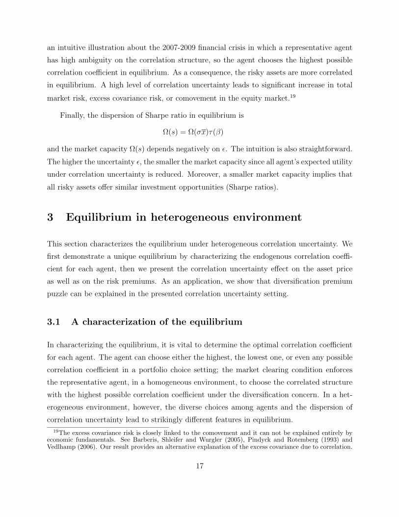
an intuitive illustration about the 2007-2009 financial crisis in which a representative agent
has high ambiguity on the correlation structure, so the agent chooses the highest possible
correlation coefficient in equilibrium. As a consequence, the risky assets are more correlated
in equilibrium. A high level of correlation uncertainty leads to significant increase in total
market risk, excess covariance risk, or comovement in the equity market.19
Finally, the dispersion of Sharpe ratio in equilibrium is
Ω(s) = Ω(σx)τ(β)
and the market capacity Ω(s) depends negatively on ε. The intuition is also straightforward.
The higher the uncertainty ε, the smaller the market capacity since all agent’s expected utility
under correlation uncertainty is reduced. Moreover, a smaller market capacity implies that
all risky assets offer similar investment opportunities (Sharpe ratios).
3 Equilibrium in heterogeneous environment
This section characterizes the equilibrium under heterogeneous correlation uncertainty. We
first demonstrate a unique equilibrium by characterizing the endogenous correlation coeffi-
cient for each agent, then we present the correlation uncertainty effect on the asset price
as well as on the risk premiums. As an application, we show that diversification premium
puzzle can be explained in the presented correlation uncertainty setting.
3.1 A characterization of the equilibrium
In characterizing the equilibrium, it is vital to determine the optimal correlation coefficient
for each agent. The agent can choose either the highest, the lowest one, or even any possible
correlation coefficient in a portfolio choice setting; the market clearing condition enforces
the representative agent, in a homogeneous environment, to choose the correlated structure
with the highest possible correlation coefficient under the diversification concern. In a het-
erogeneous environment, however, the diverse choices among agents and the dispersion of
correlation uncertainty lead to strikingly different features in equilibrium.
19The excess covariance risk is closely linked to the comovement and it can not be explained entirely byeconomic fundamentals. See Barberis, Shleifer and Wurgler (2005), Pindyck and Rotemberg (1993) andVedlhamp (2006). Our result provides an alternative explanation of the excess covariance due to correlation.
17

We define several auxiliary functions to capture the parameters ν, β1, β2 in a hetero-
geneous economy. Put
K(β1) ≡1
1−β1 −Ω(σx)
1+(N−1)β1+ (1−ν)(1−Ω(σx))
ν
11−β1 + (N−1)Ω(σx)
1+(N−1)β1
. (14)
and for each real number x, y 6= 1,− 1N−1
,
m(x, y) ≡ ν
1− x+
1− ν1− y
, n(x, y) ≡ νx
(1− x)(1 + (N − 1)x)+
(1− ν)y
(1− y)(1 + (N − 1)y). (15)
Proposition 3 The market equilibrium is presented in two separable cases.
1. (Full Participation Equilibrium) If β1 is large enough such that
β1 ≥1
N − 1
ν
1− νΩ(σx)
1− Ω(σx)N − 1
, (16)
or if β2 is strictly smaller than K(β1), there exists a unique equilibrium in which each
agent chooses the corresponding highest correlation coefficient, respectively.
2. (Limited Participation Equilibrium) If Equation (16) fails and β2 is larger than K(β1),
there exists a unique equilibrium in which the sophisticated agent chooses her highest
possible correlation coefficient β1 while the choice of the naive agent is irrelevant. How-
ever, the naive agent’s optimal demand x(n), is uniquely determined by the endogenous
Sharpe ratios in the equilibrium.
3. In either equilibrium, the market price for asset i is, for each i = 1, · · · , N ,
pi = ai −γσi
m(β1, ρ2)
(σixi +
n(β1, ρ2)
m(β1, ρ2)−Nn(β1, ρ2)
N∑j=1
σjxj
). (17)
where ρ2 = β2 in the full participation equilibrium and ρ2 = K(β1) in the limited partic-
ipation equilibrium. Furthermore, each risky asset is priced at discount in equilibrium.
That is, pi < ai and si > 0 for each i = 1, · · · , N .
18
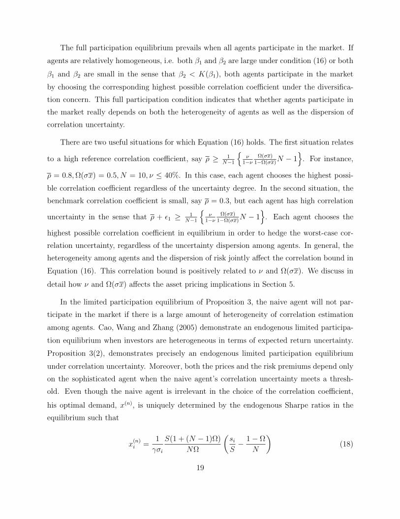
The full participation equilibrium prevails when all agents participate in the market. If
agents are relatively homogeneous, i.e. both β1 and β2 are large under condition (16) or both
β1 and β2 are small in the sense that β2 < K(β1), both agents participate in the market
by choosing the corresponding highest possible correlation coefficient under the diversifica-
tion concern. This full participation condition indicates that whether agents participate in
the market really depends on both the heterogeneity of agents as well as the dispersion of
correlation uncertainty.
There are two useful situations for which Equation (16) holds. The first situation relates
to a high reference correlation coefficient, say ρ ≥ 1N−1
ν
1−νΩ(σx)
1−Ω(σx)N − 1
. For instance,
ρ = 0.8,Ω(σx) = 0.5, N = 10, ν ≤ 40%. In this case, each agent chooses the highest possi-
ble correlation coefficient regardless of the uncertainty degree. In the second situation, the
benchmark correlation coefficient is small, say ρ = 0.3, but each agent has high correlation
uncertainty in the sense that ρ + ε1 ≥ 1N−1
ν
1−νΩ(σx)
1−Ω(σx)N − 1
. Each agent chooses the
highest possible correlation coefficient in equilibrium in order to hedge the worst-case cor-
relation uncertainty, regardless of the uncertainty dispersion among agents. In general, the
heterogeneity among agents and the dispersion of risk jointly affect the correlation bound in
Equation (16). This correlation bound is positively related to ν and Ω(σx). We discuss in
detail how ν and Ω(σx) affects the asset pricing implications in Section 5.
In the limited participation equilibrium of Proposition 3, the naive agent will not par-
ticipate in the market if there is a large amount of heterogeneity of correlation estimation
among agents. Cao, Wang and Zhang (2005) demonstrate an endogenous limited participa-
tion equilibrium when investors are heterogeneous in terms of expected return uncertainty.
Proposition 3(2), demonstrates precisely an endogenous limited participation equilibrium
under correlation uncertainty. Moreover, both the prices and the risk premiums depend only
on the sophisticated agent when the naive agent’s correlation uncertainty meets a thresh-
old. Even though the naive agent is irrelevant in the choice of the correlation coefficient,
his optimal demand, x(n), is uniquely determined by the endogenous Sharpe ratios in the
equilibrium such that
x(n)i =
1
γσi
S(1 + (N − 1)Ω)
NΩ
(siS− 1− Ω
N
)(18)
19

where Ω = τ(K(β1)) is the dispersion of Sharpe ratios.
Both the heterogeneity of agents and the dispersion of risk are involved in the limited
participation equilibrium as well. When the sum of sophisticated agents and the risk dis-
persion, ν + Ω(σx), is greater than 1, condition (16) fails. Further if the naive agent is
very uncertain about the correlation coefficient such that ε2 > K(ρ + ε1) − ρ, he decides
not to participate in the market, or equivalently, any choice of the correlation coefficient in
his plausible range is irrelevant in equilibrium. This indicates that when there are many
sophisticated agents in the market, naive agents are squeezed out of the market. As a result,
sophisticated agents dominate the trading in the market. It is also the case that when the
naive agent has a big uncertainty issue, no-diversification becomes his optimal strategy. As
explained in the portfolio choice context, if his plausible correlation coefficient range is large
enough to include τ(Ω(s)) and since τ(Ω(s)) = K(β) in equilibrium, his optimal demand
is given as xK(β), which is determined by the sophisticated agent’s endogenous correlation
coefficient β1.
Figure 1 illustrates the property of the function K(β1) with respect to β1 and how this
correlation boundary determines different equilibrium cases accordingly. As shown, the dark
curve line representing K(β1) is strictly above the straight line of β1. The limited partici-
pation equilibrium occurs only in the yellow region whereas a full participation equilibrium
happens elsewhere. As the correlation uncertainty of sophisticated investors increases, the
endogenous correlation of naive investors rises consequently.
Figure 2 illustrates the Sharpe ratios of all assets in a full participation equilibrium. The
parameters are N = 3, a1 = 50, σ1 = 9%, x1 = 5; a2 = 60, σ2 = 10%, x2 = 3.7; a3 = 15,
σ3 = 12%, x3 = 10.5. Hence Ω(σx) = 0.41. As seen in Figure 3, the plot displays similar
magnitude of the correlation-uncertainty premium as in a homogeneous environment (Table
1). The correlation-uncertainty premium can also be identified in Table 2 for a limited
participation equilibrium.
20
3.2 Diversification Premium
In this section we demonstrate that the correlation uncertainty could lead to diversification
premium under certain circumstances due to the heterogeneity among the agents and the
correlation uncertainty.
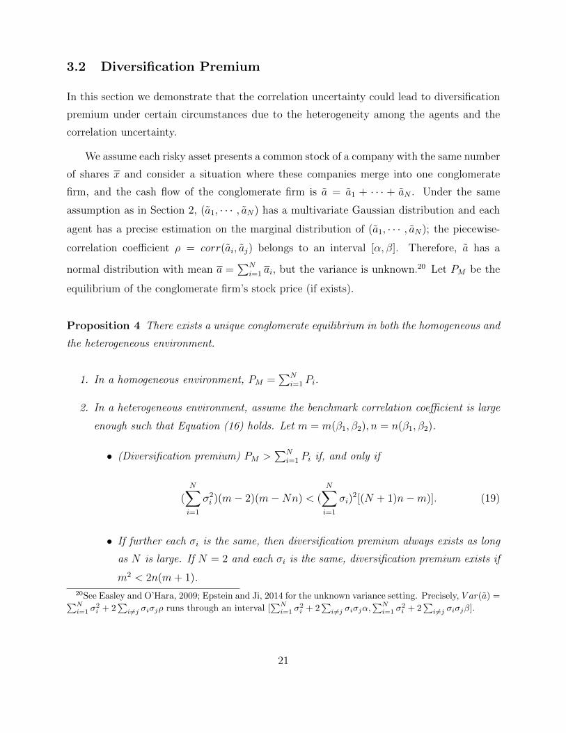
We assume each risky asset presents a common stock of a company with the same number
of shares x and consider a situation where these companies merge into one conglomerate
firm, and the cash flow of the conglomerate firm is a = a1 + · · · + aN . Under the same
assumption as in Section 2, (a1, · · · , aN) has a multivariate Gaussian distribution and each
agent has a precise estimation on the marginal distribution of (a1, · · · , aN); the piecewise-
correlation coefficient ρ = corr(ai, aj) belongs to an interval [α, β]. Therefore, a has a
normal distribution with mean a =∑N
i=1 ai, but the variance is unknown.20 Let PM be the
equilibrium of the conglomerate firm’s stock price (if exists).
Proposition 4 There exists a unique conglomerate equilibrium in both the homogeneous and
the heterogeneous environment.
1. In a homogeneous environment, PM =∑N
i=1 Pi.
2. In a heterogeneous environment, assume the benchmark correlation coefficient is large
enough such that Equation (16) holds. Let m = m(β1, β2), n = n(β1, β2).
• (Diversification premium) PM >∑N
i=1 Pi if, and only if
(N∑i=1
σ2i )(m− 2)(m−Nn) < (
N∑i=1
σi)2[(N + 1)n−m)]. (19)
• If further each σi is the same, then diversification premium always exists as long
as N is large. If N = 2 and each σi is the same, diversification premium exists if
m2 < 2n(m+ 1).
20See Easley and O’Hara, 2009; Epstein and Ji, 2014 for the unknown variance setting. Precisely, V ar(a) =∑Ni=1 σ
2i + 2
∑i6=j σiσjρ runs through an interval [
∑Ni=1 σ
2i + 2
∑i 6=j σiσjα,
∑Ni=1 σ
2i + 2
∑i6=j σiσjβ].
21

Proposition 4 shows that the heterogeneous beliefs on correlation uncertainty plays a
crucial role in the diversification premium puzzle. While the diversification discount can
be explained in a heterogeneous mean uncertainty setting in Cao, Wang and Zhang (2005),
and well documented in Janan, Servaes and Zingales (2000), recent literature also identify
diversification premium in many situations. For example, Villalonga (2004), and Hoechle, et.
al (2012), etc. Proposition 4 demonstrates that there is diversification premium when two
identical firms are merged and m2 < 2n(m+ 1) is satisfied. For instance, when Ω(σx) = 0.5
and the benchmark correlation coefficient ρ = 0.7, ν = 0.8 and the sophisticated agent has a
perfect knowledge about the correlation coefficient. Then m < 2 as long as ε ≤ 0.06 for the
naive agent. Hence, m2 < 2n(m+ 1) holds naturally and there is a diversification premium.
We also observe the diversification premium feature when the number of identical firms is
large.
3.3 Sharpe ratio and the market capacity
In this section we describe properties of the endogenous risk premium, Sharpe ratios and the
market capacity in the setting. These properties are presented by the following proposition.
Proposition 5 For each asset i 6= j,
1. si ≥ sj if, and only if σixi ≥ σjxj; It is also equivalent to σix(s)i ≥ σjx
(s)j as well as
σix(n)i ≥ σjx
(n)j , where x(j) is the optimal demand vector for the agent j ∈ s, n.
2. si is larger than the average Sharpe ratio, SN
, if and only if σixi ≥ LN
;
3. If σxiL≤ 1
Nfor asset i, then the higher the level of uncertainty for the agents the smaller
the Sharpe ratio for the asset i; the effect of correlation uncertainty on the Sharpe ratio
of asset with higher risk, σxiL> 1
Nis ambiguous.
4. Ω(s) depends negatively on the level of correlation uncertainty, but it increases with
respect to the number of sophisticated agents.
22

Proposition 5 first demonstrates the symmetric property between the Sharpe ratio with
the associated risk among all assets. Proposition 5(1) states that the a higher Sharpe ratio
always corresponds to a higher risk among all risky assets, and each agent invests more on
the assets with higher Sharpe ratios. Specially, if we re-order the risky assets i = 1, · · · , N
in the decreasing order by σixi, i = 1, · · · , N , both the sequence σix(s)i and σix
(n)i depict a
similar decreasing feature. We discuss in details about these two optimal portfolios in the
next section.
To understand Proposition 5(2) and (3), we decompose the Sharpe ratio of risky asset i
into two components:
si =S
N+γ
m
(σixi −
L
N
)(20)
where the first component is the average Sharpe ratio, and the second one represents how
much it differs from the average Sharpe ratio. We call the second component as a specific
Sharpe ratio. According to this decomposition, the specific Sharpe ratio of asset i is propor-
tional to the difference between the individual risk and the average risk, σixi − LN
, and the
endogenous Sharpe ratio is determined jointly by the average Sharpe ratio and the specific
Sharpe ratio.
Proposition 5(2) follows from Equation (20) immediately that a risky asset’s Sharpe ratio
is above the average Sharpe ratio only when its risk is above the average level. Proposition
5(3) displays the crucial difference between asset with high risk and low risk. We first
note that both the average Sharpe ratio and m(β1, ρ2) depend negatively on the level of
uncertainty,21 For an asset with low risk, σixi ≤ LN
, the specific Sharpe ratio also inversely
depends on the level of uncertainty. Therefore, when the correlation uncertainty increases,
the Sharpe ratio decreases.
However, for high risk assets, the effect of correlation uncertainty is ambiguous since
it depends on two opposing effects of the average Sharpe ratio and the specific Sharpe
ratio. With increasing uncertainty, the average Sharpe ratio decreases, and the Sharpe ratio
21It can be seen easily by the expression of m(x, y), n(x, y) and the fact that S = γLm(x,y)−Nn(x,y) and
β1 < ρ∗2 in Proposition 3.
23

decreases only when the specific Sharpe ratio is very large such that
− ∂
∂β
(1
m
)(σixi −
L
N
)>
∂
∂β
(1
m−Nn
).
Otherwise, if σixi− LN
is fairly small, the positive effect of the specific Sharpe ratio dominates
the negative effect of the average Sharpe ratio, thus reaching a positive impact in total.
The intuition of Proposition 5(4) also follows in essence from the above decomposition of
the Sharpe ratio. Reformulate Equation (20) as a multiplication version of the decomposition
of the Sharpe ratio in terms of the average Sharpe Ratio.
siS− 1
N=m−Nn
m
(σixiL− 1
N
). (21)
Since m−Nnm
is negatively related to the correlation uncertainty22, the sensitivity of the relative
Sharpe ratio siS
relies on σixiL− 1
N: it decreases for assets with σixi
L> 1
N, and increases for
assets with σixiL
< 1N
. By Proposition 5, (2), σixiL
> 1N
is associated with siS> 1
N. Therefore,
with increasing correlation uncertainty, siS
decreases if siS> 1
Nand increases if si
S< 1
N. Put
it together, all siS
are closer with higher correlation uncertainty, so the dispersion of Sharpe
ratio decreases, as presented in Proposition 5, (4).
4 Optimal portfolios
In this section we discuss and compare the optimal portfolio, x(s) and x(n). Our comparison
between these two optimal portfolios is summarized by the next proposition.
Proposition 6 1. (Underdiversification and well-diversification). Comparing with the
market portfolio∑N
i=1 xiai, the naive agent has an underdiversified portfolio while the
sophisticated agent has a more diversified (well-diversification) portfolio.
22By the proof of Proposition 3, m−Nnm = k(β1, ρ2) in Appendix, Equation (A-17), and it is easy to checkits property as desired.
24

2. (Portfolio Risk) The sophisticated agent holds a riskier portfolio than the naive agent.
Specifically, the variance of∑
i aix(s)i is strictly larger than the variance of
∑i aix
(n)i .
3. (Portfolio Position) The sophisticated agent holds long position on all risky assets; the
naive agent hold long positions only on the high risk assets and short positions on the
low risk positions.
4. (Portfolio Performance) The sophisticated agent has a better portfolio performance than
the naive agent in the sense that the Sharpe ratio of her optimal portfolio is strictly
larger than the Sharpe ratio of the naive agent’s optimal portfolio.
5. (Maxmin Expected Utility) The sophisticated agent has a higher maxmin expected utility
than the naive agent.
6. (Comovement) From both the sophisticated agent and the naive agent’s perspective, the
optimal portfolios have a comovement feature. Specifically, the covariance of these two
optimal portfolios are greater than ( SN
)2, which is always positive.
Proposition 6, (1), demonstrates that, in a precise manner, the sophisticated agent al-
ways chooses a more diversified optimal portfolio than the naive agent, and it sheds some
lights on the underdiversification puzzle. Compared with the market portfolio, the naive
agent’s portfolio is always under-diversified according to the dispersion measure while the
sophisticated agent has a more diversified portfolio.
It is well documented that underdiversification can happen due to model misspecifica-
tion (Uppal and Wang, 2003; Easley and O’Hara, 2009), heterogeneous beliefs (Milton and
Vorkink, 2008). For instance, Easley and O’Hara (2009) demonstrates limited participation
happens at the presence of the marginal distribution ambiguity while assets are assumed
to be independent. Uppal and Wang (2003) considers the ambiguity for both the joint dis-
tribution and the marginal distributions from a portfolio choice setting. Uppal and Wang
(2003) shows that numerically, when the overall ambiguity about the joint distribution is
high, a small difference in ambiguity for the marginal return distribution will result in an
under-diversified portfolio. By contrast, our result shows that underdiversification can be
generated endogenously from the dispersion of correlation uncertainty, even without ambi-
guity on any marginal distribution. In a particular case, the naive agent could even hold
25

a limited participation portfolio when his ambiguity on the correlated structure is large
enough.23 Furthermore, we demonstrate a well-diversified portfolio is associated with a so-
phisticated agent given her sophistication on the correlated structure estimation.
We draw numerically the dispersion of the sophisticated agent’s and the naive agent’s
optimal portfolio in Figure 8. Figure 8 is concerned with a full participation equilibrium in a
heterogeneous setting. Clearly, the dispersion of the sophisticated agent’s optimal portfolio,
as drawn in the upper plot, is smaller than the corresponding dispersion of the naive agent’s
optimal portfolio in the lower plot.
To show further the application of the dispersion measure to the limited participation, we
consider a limited participation equilibrium and compute the optimal portfolio’s dispersion
for each agent, in Table 3. As shown, the naive agent’s dispersion is fairly close to one,
which reflects to his extremely under-diversified portfolio. By contrast, the dispersion of
the sophisticated agent’s optimal portfolio is between 0.625 and 0.629, indicating a more
diversified holding.
Proposition 6, (2) concerns with the portfolio risk, which states that the sophisticated
agent is willing to take a riskier portfolio than the naive agent due to the dispersion of
correlation uncertainty among agents. The intuition is simple. Since ambiguity-aversion
leads to risk-aversion, the naive agent behaves more risk-averse; hence, he has a smaller
risk in his optimal portfolio. Proposition 6, (2), demonstrates that ambiguity-aversion leads
to risk-aversion in the correlated structure,24 and a higher level of correlation uncertainty
yields a higher level of risk-aversion; thus the corresponding optimal portfolio is less risky.
The comparison of portfolio risk can be also derived by Proposition 6, (3) which gives the
position on each risky asset. Actually, by the explicit expression of x(s), x(n) in Proposition
3 and Proposition 1, the sophisticated agent holds all long positions on all risky assets but
the naive agents might hold short positions on some risky asset. Therefore, the sophisticated
agent’s portfolio risk is higher.
Proposition 6, (4)-(5) further compare the performance between these two optimal port-
folios. As expected, the sophisticated agent has a higher Sharpe ratio portfolio than the
23See Mankiw and Zeldes (1991) and Vissing-Jorgensen (2003).24It is well known that uncertainty aversion yields risk aversion in the ambiguity literature. See Easley
and O’Hara (2008, 2012); Cao, Wang and Zhang (2005); Gollier (2011); Garlappi, Uppal and Wang (2012).
26

naive agent. By the same token, the sophisticated agent also has a higher maxmin expected
utility.
At last, Proposition 6, (6), investigates the comovement between the agents from their
own perspectives and we observe a robust comovement pattern among the agents (See Simsek,
2013 and Towensend, 1994 for a comovement among householders’ optimal equity portfolios).
5 Sophisticated agents and risk dispersion
In this section we examine the implication of sophisticated agents and risk dispersion. ν
represents the percentage of sophisticated agent or institutional investor. σixi represents
the total risk of the firm to the market. It is different from the volatility σi or the market
capitalization pixi that are often used as proxies of stock characteristics. We use Ω(σx) to
represent the risk dispersion in the economy. We derive several testable hypothesis in this
regard. To emphasize the impact of ν,Ω(σx) we highlight on these two variables as extra
components in this section.
5.1 Sophisticated agents
We first discuss the effect to the equilibrium. For this purpose, we let
L(β1) = limν→1
K(β1, ν) =1− Ω(σx) + β1(Ω(σx) +N − 1)
1 + (N − 1)Ω(σx) + (N − 1)β1(1− Ω(σx))
If both agents have fairly close correlation uncertainty that β2 is smaller than L(β1), then
β2 ≤ K(β1, ν) regardless of the amount of sophisticated agents and therefore, by Proposition
3, there is a full participation equilibrium. The number of sophisticated agent has significant
effect on equilibrium if the level of correlation uncertainty differs from each, say, β2 > L(β1).
For a small number of sophisticated agents, β2 ≤ K(β1, ν). However, if there are so many
sophisticated agents that β2 > K(β1, ν), a limited participation equilibrium prevails. In
an extreme case, ν → 1, the limited participation equilibrium becomes the homogeneous
equilibrium as in Proposition 2.
27

Proposition 7 1. (Equilibrium) If β2 ≤ L(β1), there exists no limited participation.
However, if β2 > L(β1), there is only limited participation equilibrium as long as there
are many sophisticated agents.
2. (Price) If σixiL≤ 1
Nfor asset i, then ∂
∂ν(si) < 0, ∂
∂ν(pi) > 0. The effect of ν on the price
is ambiguous for asset i with σixiL
> 1N
.
3. (Volume) If σixiL≤ 1
Nfor asset i, then x
(s)i > x
(n)i , and ∂
∂νx
(s)i < 0, ∂
∂νx
(n)i < 0. On the
other hand, if σixiL≥ 1
N, then ∂
∂ν
(νx
(s)i
)> 0.
Proposition 7, (1) follows directly from the above discussion. Proposition 7, (2) follows
from the decomposition of the Sharpe ratio, Equation (A-31) and its intuition is similar to
Proposition 5, (2). Proposition 7 further justifies the impact of institutional investors on the
price from the demand perspective. The sophisticated agent has higher demand on the low
risk assets than the naive agent, leading to a price increase of the low risk asset. It is also
interesting to see that with increasing sophisticated agent, the total volume increases on the
high risk asset. However, regarding the individual demand for each agent, the impact of ν on
the high risk asset is not as clear as it is on the low risk asset. Furthermore, the demand of
the sophisticated agent on the low risk asset depends on two opposite effects of the average
Sharpe ratio and the specific Sharpe ratio; thus the effect of ν is ambiguous.
5.2 The risk dispersion Ω(σx)
The market risk distribution Ω(σx) performs another vital role in the heterogeneous equi-
librium and displays important asset pricing implications from several aspects.
First, the level of Ω(σx) affects the market equilibrium. When each firm (risky assets)
contributes the similar risk to the market, it generates a full participation equilibrium. In
one extreme case, if each risky asset contributes the same risk, Ω(σx) = 0, then Ω(s) = 0. On
the other hand, when the risky assets contribute very different contribution, or alternatively,
they offers a skewed risk distribution and Ω(σx) is close to one, a limited participation
28

equilibrium is generated. To understand it, we observe that
limΩ(σx)→1
K(β1,Ω(σx)) = β1. (22)
Therefore, any naive agent with β2 > β1 must hold a limited portfolio for a skewed enough
risk distribution, that is, Ω(σx) is close enough to one.
Our analysis regarding the risk dispersion demonstrates another channel for the limited
participation phenomena, which can be generated due to a large risk dispersion. For instance,
if the equity market and the bond market contributes a far different risk, naive agents or
households (retail investors) want to optimally hold a limited participation portfolio. As
another example, if one country (say, U.S. equity market) dominates other equity markets
in an international setting, households want to focus on the investment on the U.S equity
market and there is no much incentive to participate in the international market.
Second, the Sharpe ratios and the dispersion of Sharpe ratios (the market capacity)
depend on the risk distribution. Equation (A-15) presents this fundamental relationship. In
both the full participation and the limited participation equilibrium (by Equation A-32) ,
we have
∂Ω(s)
∂Ω(σxi)> 0. (23)
Due to this positive relation, the higher the risk dispersion the higher the market capacity.
6 Extension
So far, we assume that any two risky assets have the same, or very close, correlation coeffi-
cient. In this section, we justify this assumption first and then present its extensions.
We consider a two-period economy with N risky assets and one zero supply risk-free
asset, and these N risky assets follow a one factor model such as ai = βim + ε where
m represents one fundamental factor and each εi is the specific risk for the asset i. The
correlation coefficient between the asset i and asset j is
corr(a,aj) =(βiσm)(βjσm)√
(βiσ2m + σ2
i )(βjσ2m + σ2
j ).
29

Thus, this correlated structure is one special case of a correlated structure in which corr(ai, aj) =
bibj,∀i 6= j for a sequence of positive numbers b1, · · · , bN . If in particular, b1 = · · · = bN ,
the correlation matrix becomes R(ρ) in Section 2. The general situation can be studied in a
portfolio choice setting as in proposition 1.
As another example and without relying the factor-model, we decompose these risky
assets are decomposed into K sectors based on their firm characterizes, business and so
on. Therefore, the risky assets in each factor have relatively close correlation coefficient.
Specifically, we group assets into several classes, A1, A2, · · · , Ak, such that the piece-wise
correlation coefficients among assets in each class Ai is very close to each other and the
common correlation coefficient is denoted by ρi. We assume that ρ1 >> ρ2 >> · · · >> ρk.
25 In this way, ρ1 represents the largest possible correlation coefficient among all assets
and any pair of assets in class A1 has a correlation coefficient (or very close to) ρ1. The
correlation coefficient ρ2 denotes the second largest possible correlation coefficient, to some
contexts, among all assets in the market. For this reason we assume that ρ1 dominates ρ2,
written as ρ1 >> ρ2.
Under the above hierarchical correlation structure, we are able to extend the model set-
ting in Section 2 to each asset class A1, A2, · · · , Ak separably, since the piece-wise correlation
coefficient in each asset class Ai is fairly close to each other. In fact, this result can be applied
to any asset class in which the piece-wise correlation coefficient is close to each other, when
the correlation uncertainty within this asset class is a concern. For instance, because of the
too big to fail issue and the substantial systemic risk, it is essential to understand the cor-
relation structure among these big financial institutions as a group and how it changes with
respect to macro-economic shocks26. Therefore, to investigate the correlation uncertainty
among those big financial institutions is important and our previous results can be applied
virtually in this setting.
To demonstrate our extended setting, we consider two different correlated structures
among asset classes in the hierarchical structure. In the first one, we assume that each asset
25We use a >> b to represent that the number a is way larger than b. This decomposition of the correlationstructure is similar to the principal component analysis in which the eigenvalues of the covariance matrixhas a decreasing order in terms of “>>”.
26For instance, for big financial institutions such as Bank of America, Citi, AIG, Wells Fargo, JP Morgan,our computation shows that any pair of two big financial institutions in this group stays between 70% to80% from 2001 to 2014, including pre-crises and post-crisis time period.
30

class is independent to each other, or have extremely small correlation coefficients at the
least. For simplicity we use two asset classes to illustrate, the correlation matrix can be
written as
R1 =
[R(ρ1) 0
0 R(ρ2)
].
with ρ1 >> ρ2 and each R(ρi) is a correlation matrix with element ρi off the diagonal and
the component being one along the diagonal.
For the second correlated structure, we consider two asset classes while the first asset
class contains asset i ∈ I and the second asset class contains all other assets j ∈ J . Given the
hierarchical structure, we assume that for each pair i1 6= i2 ∈ I, corr(ai1 , ai2) = ρ1, and for
each pair j1 6= j2 in J , corr(aj1 , aj2) = ρ2. We assume that ρ1 >> ρ2. Since the correlation
between asset class I and asset class J is not substantial, we assume that corr(ai, aj) = ρ1ρ2
for i ∈ I, j ∈ J . Precisely, the correlation matrix is written as27
RII =
[R(ρ1) ρ1ρ2Bρ1ρ2B
′ R(ρ2)
].
with ρ1 >> ρ2 and R(ρ1) is a M ×M matrix, R(ρ2) is a J × J matrix and B is a M × Jmatrix with components one. Since we are interested in the positive correlated environment,
we assume that ρi > 0 for each i = 1, · · · , K in each correlated structure.
Proposition 8 In a homogeneous environment the representative agent has a correlation
uncertainty [ρk − εk, ρk + εk] on the correlation coefficient ρk in the asset class Ak for k =
1, 2. We assume that the correlation uncertainty is also consistent with the correlated struc-
ture in the sense that ρ1−ε1 > ρ2+ε2 for the first hierarchical structure, and ρ1−ε1 >> ρ2+ε2.
The agent chooses the highest possible correlation coefficients in equilibrium in the above two
correlation structures with correlation uncertainty.
According to Proposition 8, the representative agent chooses the highest plausible cor-
relation coefficients in a relatively straightforward hierarchical correlated structure. Similar
27We can check that R2 is a positive definite matrix largely, thus, R2 is a correlation matrix for a multi-variate Gaussian variable.
31
to our previous discussion in Section 1, ρk + εk relies on both the benchmark and the level of
correlation uncertainty for each asset class Ak. In an extremely weak market situation where
the level of correlation uncertainty is high, the endogenous correlation coefficients between
assets will be high, and the endogenous risk premiums will increase and prices will drop
enormously. Therefore, our previous arguments can be applied to the general correlation
structure.
The endogenous correlation pattern in hierarchical correlated structure is richer than
the one exhibited in Section 6, attributable to the heterogeneous uncertainty levels among
agents. The endogenous market correlation is time-varying, depending on the benchmark
of the correlation coefficients in each asset class and the level of uncertainty. Besides, the
endogenous correlation inside each asset class or between asset classes increase with the
number of sophisticated agents.
7 Conclusion
To investigate the on-going complicated correlation structure among asset classes and the
nature of well-documented empirical correlated-related facts, this paper develops an equi-
librium model at the presence of correlation uncertainty where two types of agents have
heterogeneous beliefs in their correlation estimation. We find that those correlation-related
phenomena can be essentially connected through the disagreement among agents in the corre-
lation structure, the dispersion of the agents and assets’ risk, when the marginal distribution
of each risky asset is a perfect knowledge.
Specifically, when the disagreement on correlation estimation is large, the naive agent
does not participate in the market, thus a limited participation equilibrium. This is also
true when more sophisticated agents emerge in the market or when the dispersion of assets’
risk is high. The naive agent is irrelevant to choose his correlation coefficient even though
his optimal portfolio is uniquely determined in equilibrium. Our portfolio analysis demon-
strates that the sophisticated agent always holds a diversified portfolio in contrary to the
naive agent who is underdiversified. Our equilibrium model is helpful to explain asymmetric
correlation, correlation trading, comovement and diversification premium (discount). This
paper contributes further to the literature on the asset pricing implication of Knightian
uncertainty.
32

Appendix A: Proof
The following Sherman-Morrison formula in linear algebra is useful in the subsequent deriva-
tions.
Lemma 1 Suppose A is an invertible s×s matrix and u, v are s×1 vectors. Suppose further
that 1 + vTA−1u 6= 0. Then the matrix A+ uvT is invertible and
(A+ uvT )−1 = A−1 − A−1uvTA−1
1 + vTA−1u. (A-1)
The next lemma computes the dispersion of optimal demand in terms of the dispersion
of the Sharpe ratios.
Lemma 2 Let ρ 6= 1, ρ 6= − 1N−1
. Then
Ω(σxρ) = Ω(s)1 + (N − 1)ρ
1− ρ; Ω(s) = Ω(σxρ)
1− ρ1 + (N − 1)ρ
(A-2)
Proof. Note that σxρ = 1γR(ρ)−1s. By Lemma 1,
R(ρ)−1 =1
1− ρIN −
1
1 + (N − 1)ρ
ρ
1− ρeeT . (A-3)
Then Ω(σxρ) = Ω(t), where ti = si − ρ1+(N−1)ρ
S. We obtain∑N
i=1 ti = 1−ρ1+(N−1)ρ
S, and
N∑i=1
t2i =N∑i=1
(s2i − 2siS
ρ
1 + (N − 1)S+
(ρ
1 + (N − 1)ρ
)2
S2
)
=N∑i=1
s2i −
(N − 2)ρ2 + 2ρ
(1 + (N − 1)ρ)2S2.
By straightforward computation, we obtain
Ω(t) = Ω(s)1 + (N − 1)ρ
1− ρ. (A-4)
33

Proof of Proposition 1.
By Sion’s theorem (1958),
A = maxx∈RN
minρ∈[α,β]
(ai − pi)xi −
1
2
N∑i,j=1
xixjσiσjRij
= B ≡ minρ∈[α,β]
maxx∈RN
(ai − pi)xi −
1
2
N∑i,j=1
xixjσiσjRij
and both A and B are equal to minρ∈[α,β]1
2γG(ρ), where
G(ρ) ≡ sTR−1s =N∑N
n=1 s2n − (
∑Nn=1 sn)2
N(1− ρ)+
(∑N
n=1 sn)2
N(1 + (N − 1)ρ). (A-5)
G(ρ) can be rewritten in term of the dispersion measure as follows.
G(ρ) =S2
N
((N − 1)Ω(s)2
1− ρ+
1
1 + (N − 1)ρ
).
Lemma 3 Notations as above. The solution of minρ∈[α,β] G(ρ) is given by
ρ∗ =
α, if α > τ(Ω(s)),β, if β < τ(Ω(s)),τ(Ω(s)) if τ(Ω(s)) ∈ [α, β].
(A-6)
Proof of Lemma 3. For simplicity we assume that Ω(s) 6= 1N−1
and let τ(Ω(s)) ≡1+Ω(s)
1−(N−1)Ω(s). Then,
G′(ρ) =(N − 1)S2
N(1− ρ)2[1 + (N − 1)ρ]2[Ω(s)2(N − 1)2 − 1][ρ− τ(Ω(s))][ρ− τ(Ω(s))]. (A-7)
Thus, ρ∗ = argminρ∈[α,β]G(ρ) is determined in the following three cases, respectively.
34

• If Ω(s) ≥ 2N−2
, then |τ(Ω(s))| ≤ 1, |τ(Ω(s))| ≤ 1 and τ(Ω(s)) < τ(Ω(s)). Moreover
τ(Ω(s)) ≤ 0 ≤ α.
• If 2N−2
> Ω(s) > 1N−1
, then τ(Ω(s)) < −1, and 0 < τ(Ω(s)) < 1.
• If Ω(s) < 1N−1
, then |τ(Ω(s))| ≤ 1, τ(Ω(s)) > 1; but Ω(s)2(N − 1)− 1 < 0 so G′(ρ) =
(−)× (ρ− τ(Ω(s)))× (ρ− τ(Ω(s))).
Then the proof of Lemma 3 is finished.
Proof of Proposition 1, Continue.
By the above argument, we have shown that
A = B =1
2γG(ρ∗) = CE(ρ∗, xρ∗). (A-8)
(1). If α > τ(Ω(s)), then by Lemma 2, Ω(σxα) > 1 and maxΩ(σx)>1CE(α, x) =
CE(α, xα) = A. By equation (A-8) and the property of G(ρ) stated in Lemma 3, we know
that maxΩ(σx)<1CE(β, x) ≤ maxxCE(β, x) < CE(α, xα). Similarly, maxΩ(σx)=1 CE(ρ, x) <
CE(α, xα) for each ρ ∈ [α, β]. Then the unique solution of the problem (2) is ρ∗ = α, and
x∗ = xα.
(2). If β < τ(Ω), by Lemma 2, maxΩ(σx)<1CE(β, x) = CE(β, xβ) = A. Moreover, by
equation (A-8) and Lemma 3, we have maxΩ(σx)>1CE(α, x) ≤ CE(α, xα) < CE(β, xβ) and
maxΩ(σx)=1 CE(ρ, x) < CE(β, xβ) for each ρ ∈ [α, β]. Therefore, ρ∗ = β, x∗ = xβ is the
unique solution of the portfolio choice problem (2).
(3). Assume that α ≤ τ(Ω) ≤ β. By equation (A-8), A = B = CE(τ(Ω(s)), xτ(Ω(s))
).
Moreover, by Lemma 2, Ω(xτ(Ω(s))
)= 1. By straightforward calculation, we have
A = B = CE(τ(Ω(s)), xτ(Ω(s))
)=
(∑
i si)2
2γ
(1 + (N − 1)Ω(s)
N
)2
.
For any x with Ω(σx) < 1, by Lemma 3 and the last equation, we have
CE(β, x) ≤ CE(β, xβ) < A = CE(τ(Ω(s)), xτ(Ω(s))
).
35

By the same reason, for any x with Ω(σx) > 1, we see that CE(α, x) < CE(τ(Ω(s)), xτ(Ω(s))
).
Finally, for each x∗ with Ω(σx∗) = 1 and CE(τ(Ω(s)), x∗) = maxΩ(σx)=1 CE(τ(Ω(s)), x∗), we
have CE(τ(Ω(s)), x∗) = CE(τ(Ω(s)), xτ(Ω(s))), and because of the uniqueness xρ for max-
imizing CE(ρ, x), x∗ = xτ(Ω(s)). Therefore, we have shown that the unique demand for
the uncertainty-averse agent is xτ(Ω(s)), but the agent is irrelevant to choose any correlation
coefficient ρ ∈ [α, β] since CE(ρ, xτ(Ω(s))) = A for each ρ ∈ [α, β].
The proof of Proposition 1 is completed.
Proof of Proposition 2.
The optimal demand x∗ is presented by Proposition 1. By the market clearing condition,
x∗ = x in equilibrium. Then Ω(σx∗) = Ω(σx). Since Ω(σx) < 1. Therefore, the optimal
demand in equilibrium satisfies Ω(σx∗) < 1. Then, by Proposition 1 again, the optimal
correlation coefficient is ρ∗ = β, the highest possible correlation coefficient.
In what follows we do not distinguish agent j = 1, 2 or j = s, n for sophisticated agent
and naive agent, respectively.
Proof of Proposition 3.
The unique optimal demand of type j = 1, 2 agent is xj = 1γσ−1R−1
j s and Rj corresponds
to an endogenous correlation coefficient ρj ∈ [αj, βj]. Note that xj is unique regardless of
the optimal correlation coefficient in Proposition 1, (3) and in this case let ρ = τ(Ω(s)). In
equilibrium, we have νx1 + (1− ν)x2 = x. Then
1
γ(νR−1
1 + (1− ν)R−12 ) · s = σx. (A-9)
The coefficient matrix of the last equation, X = νR−11 + (1− ν)R−1
2 , is written as
X ≡(
ν
1− ρ1
+1− ν1− ρ2
)IN −
(νρ1
(1− ρ1)(1 + (N − 1)ρ1)+
(1− ν)ρ2
(1− ρ2)(1 + (N − 1)ρ2)
)eeT
(A-10)
Let m ≡ ν1−ρ1 + 1−ν
1−ρ2 , n ≡νρ1
(1−ρ1)(1+(N−1)ρ1)+ (1−ν)ρ2
(1−ρ2)(1+(N−1)ρ2)and notice that m−Nn =
ν1+(N−1)ρ1
+ 1−ν1+(N−1)ρ2
> 0. Then by Lemma 1, X is invertible and its inverse matrix is (with
36

κ ≡ m−Nnm
)
X−1 =1
m
(IN +
n
κmeeT). (A-11)
Therefore, s = γX−1 · (σx). Precisely,
si =γ
m
(yi +
n
κmL), L ≡
N∑i=1
σixi. (A-12)
Hence ∑si =
γ
m
(1 +
Nn
κm
)L =
γL
m− nN(A-13)
and
∑(siγ
)2
=C2
m2+L2
m2
(Nn2
κ2m2+ 2
n
κm
)
=C2
m2+L2
m2
(2n
m−Nn+
Nn2
(m−Nn)2
)
=C2
m2+L2
m2
2mn−Nn2
(m−Nn)2
where C2 =∑N
i=1(σixi)2. Then
∑s2i
(∑si)2
=C2
L2
(m−Nn)2
m2+
2mn−Nn2
m2
=C2
L2κ2 +
1
N(1− κ2).
Therefore,
Ω(s)2 =1
N − 1
(N
∑s2i
(∑si)2− 1
)= κ2Ω(σx)2, (A-14)
and then a fundamental relationship between the dispersion of Sharpe ratios and the disper-
sion of risks as follows
Ω(s) = κΩ(σx). (A-15)
37

Assume first that Ω(σx) = 0, then each σixi = c and Equation (A-15) ensures that
Ω(s) = 0 and τ(Ω(s)) = 1. Therefore, each agent chooses her highest correlation coefficient
in equilibrium by Proposition 1. Moreover, all Sharpe ratios are the same and equal to
si =c
m
(1 +
nN
m− nN
)=
c
m− nN. (A-16)
We next assume that Ω(σx) ∈ (0, 1) and characterize the equilibrium in general. By
using Proposition 1, there are five different cases regarding the equilibrium.
Case 1: τ(Ω(s)) ≤ α2. Each agent chooses the smallest possible correlation coefficient, respec-
tively.
Case 2: α2 < τ(Ω(s)) < α1. The sophisticated agent chooses the smallest possible correlation
coefficient; the naive agent is irrelevant of the correlation coefficient and his optimal
holding is xτ(Ω(s)).
Case 3: τ(Ω(s)) ∈ [α1, β1]. Each agent is irrelevant of the correlation coefficient and the corre-
sponding optimal holding is xτ(Ω(s)).
Case 4: β1 < τ(Ω(s)) ≤ β2. The sophisticated agent chooses the highest possible correlation
coefficient; the naive agent is irrelevant of the correlation coefficient and his optimal
holding is xτ(Ω(s)).
Case 5: β2 < τ(Ω(s)), each agent chooses her highest possible correlation coefficient.
We prove next that Case 1 - Case 3 is impossible in equilibrium and characterize the
equilibrium condition in both Case 4 and Case 5.
To proceed we state a simple lemma below and investigate each case respectively. Recall
κ = κ(ρ1, ρ2) ≡ν
1+(N−1)ρ1+ 1−ν
1+(N−1)ρ2ν
1−ρ1 + 1−ν1−ρ2
. (A-17)
Lemma 4 Assume that κ = νa+(1−ν)bνc+(1−ν)d
with a, b, c, d > 0 and ν ∈ (0, 1). Then
min
a
c,b
d
≤ κ ≤ max
a
c,b
d
. (A-18)
38
The inequalities are strictly if ac6= b
d.
Case 1. We show that this situation is impossible in equilibrium. Since τ(Ω(s)) ≤ α2 <
α1 ensures that Ω(s) ≥ τ(α2) > τ(α1). Then, by Equation (A-15),
κ = κ(α1, α2) =Ω(s)
Ω(σx)> Ω(s) > τ(α1), τ(α2), (A-19)
which is impossible by Lemma 4.
Case 2. We prove that it is impossible in equilibrium in this situation that α2 <
τ(Ω(s)) ≤ α1.
In this case, τ(α2) > Ω(s) ≥ τ(α1). But
κ = κ(α1, τ(Ω(s))) > κΩ(σx) = Ω(s) ≥ 1− α1
1 + α1(N − 1), κ > Ω(s) =
1− τ(Ω(s))
1 + (N − 1)τ(Ω(s)).
(A-20)
Hence, it is impossible by using Lemma 4 again.
Case 3. We prove that it is impossible that τ(Ω(s)) ∈ [α1, β1] in equilibrium.
Otherwise, the optimal holding of each agent is xτ(Ω(s)) by Proposition 1. Then the
market clearing condition yields that xτ(Ω(s)) = x. However, by Lemma 2, Ω(σxτ(Ω(s))) = 1
but Ω(σx) < 1. Therefore, Case 3 is not possible in equilibrium.
Case 4. We characterize the equilibrium in which β1 < τ(Ω(s)) ≤ β2. In equilibrium,
ρ1 = β1, the optimal holding for the naive agent is xτ(Ω(s)), and
τ(β2) ≤ Ω(s) < τ(β1). (A-21)
By definition of κ, we have
κ = κ(β1, τ(Ω(s))) =Ω(s)
Ω(σx)=
ν1+(N−1)β1
+ 1−νN
(1 + (N − 1)Ω(s))ν
1−β1 + 1−νΩ(s)N
(1 + (N − 1)Ω(s)). (A-22)
By solving the last equation in Ω(s), we obtain
Ω(s) =
ν1+(N−1)β1
Ω(σx)− 1−νN
(1− Ω(σx))
ν1−β1 + (1−ν)(N−1)
N(1− Ω(σx))
. (A-23)
39

In particular, Ω(s) ≥ 0 ensures that
β1 ≤1
N − 1
ν
1− νΩ(σx)
1− Ω(σx)N − 1
. (A-24)
Moreover, the left side of Equation (A-21) is translated as β2 ≥ τ(Ω(s)) = K(β1), and the
right side of Equation (A-21) is K(β1) ≥ β1 which holds always. Then there exists a unique
equilibrium in Case 4, a limited participation equilibrium, under conditions presented in
Proposition 3.
Case 5. We characterize the equilibrium in which τ(Ω(s)) > β2.
In equilibrium, ρ1 = β1, ρ2 = β2, and Ω(s) < τ(β2) < τ(β1), which is equivalent to
κ(β1, β2)Ω(s) < 1−β21+(N−1)β2
. By straightforward computation, this condition equals to
ν
1− β1
+Ω(σx)ν(N − 1)
1 + (N − 1)β1
β2 <
ν
1− β1
− Ω(σx)ν
1 + (N − 1)β1
+ (1− ν)(1− Ω(σx)) (A-25)
or equivalently, β2 < K(β1).
To the end, we note that when β1 is large enough such that
Ω(σx)νN
(1− ν)(1− Ω(σx))≤ 1 + (N − 1)β1, (A-26)
or equivalently,
β1 ≥1
N − 1
ν
1− νΩ(σx)
1− Ω(σx)N − 1
,
then β2 < K(β1) holds by natural since β2 < 1. Then we have characterized the equilibrium
in Proposition 3.
Finally, by using this characterization, we see that each si > 0, thus, each risky asset is
priced at discount in equilibrium.
Proof of Proposition 4.
We first solve the portfolio choice problem under correlation uncertainty in a conglomer-
ate economy. which is virtually one economy with one risky asset in the presence of variance
40
ambiguity. It is easy to see that the optimal variance must be the largest possible vari-
ance to hedge the ambiguity concern, which in turn leads to the highest possible correlation
coefficient. Therefore, the optimal demand on the conglomerate firm is
x∗M =a− pM∑N
i=1 σ2i + 2
∑i 6=j σiσjβ
. (A-27)
(1) We first consider the homogeneous environment, x∗M = x. Then it follows from
Equation (A-27) that
pM = a− γx
N∑i=1
σ2i + 2
∑i 6=j
σiσjβ
.
By using Proposition 2, we see that PM =∑N
i=1 Pi holds,thus neither diversification discount
nor diversification premium.
(2) We consider the heterogeneous environment, the optimal demand x∗i,M for each agent
i = 1, 2 satisfies
a− pM = γx∗i,M
N∑i=1
σ2i + 2
∑i 6=j
σiσjβj
since each agent chooses the corresponding highest correlation coefficient. Since νx∗1,M +(1−
ν)x∗2,M = x, we obtain, for m = m(β1, β2), n = n(β1, β2),
a− pM =γx
m
m
N∑i=1
σ2i + 2
∑i 6=j
σiσj
. (A-28)
On the other hand, by Proposition 3, each stock’s market price, if traded separably, is
pi = ai −γx
m
σ2i + σi
n
m−Nn
N∑j=1
σj
.
Then,
N∑i=1
pi =N∑i=1
ai −γx
m
N∑i=1
σ2i +
n
m−Nn(N∑i=1
σi)2
.
41

Then,
a−N∑i=1
pi =γx
m
N∑i=1
σ2i +
n
m−Nn(N∑i=1
σi)2
. (A-29)
Therefore, pM >∑N
i=1 pi if, and only if
(N∑i=1
σi)2[(N + 1)n−m] >
N∑i=1
σ2i (m− 2)(m− nN).
In particular, if each σi is the same, the last formula is equivalent to
N [(N + 1)n−m] > (m− 2)(m−Nn)
which obviously holds when N is large enough. The proof of Proposition 4 is completed.
Proof of Proposition 5.
The first part of (1) follows from the characterization of the Sharpe ratio in Proposition
3. The statement for the sophisticated agent follows from the expression of σix(s)i :
γσix(s)i =
1
1− β1
si −
β1
1 + (N − 1)β1
S
. (A-30)
Then, σix(s)i ≥ σjx
(s)j if and only if si ≥ sj. The proof for the naive agent is the same.
As explained in the text, both (2) and (3) follows from the following decomposition of
the Sharpe ratio
si =S
N+γ
m
(σixi −
L
N
). (A-31)
For (4), according to Equation (A-15), Ω(s) = κΩ(σx). In the limited participation
equilibrium, we have
Ω(s) =
Ω(σx)νN1+(N−1)β1
− (1− ν)(1− Ω(σx))νN
1−β1 + (1− ν)(1− Ω(σx))(N − 1). (A-32)
Clearly, ∂Ω(σx)∂β1
< 0 and ∂Ω(σx)∂ν
> 0. The proof for the full participation equilibrium follows
from the fact that κ(ρ1,ρ2)∂ρ1
< 0, κ(ρ1,ρ2)∂ρ2
< 0, and κ(ρ1,ρ2)∂ν
> 0.
42

(3). We have
∂
∂β
(siS
)=
∂
∂β
( nm
)(1−N σixi
L
). (A-33)
By formula (A-15), ∂∂β
(nm
)= −Ω(s)
N∂Ω(s)∂β
. By Proposition 5, (4), ∂Ω(s)∂β
< 0 in equilibrium and
equilibrium B where β is the corresponding endogenous correlation coefficient(s). Therefore,
∂∂β
(nm
)> 0. By the same argument we can show that ∂Ω(s)
∂ν> 0. The proof of Proposition 5
is finished.
Proof of Proposition 6.
(1). We compare the agents’ optimal portfolios with the market portfolio in term of
the market capacity Ω(s). First, Equation (A-15) states that Ω(s) = κΩ(σx). In the full
participation equilibrium, Lemma 2 implies that Ω(s) = Ω(σx(j))1−ρj
1+(N−1)ρj. Then, by Lemma
4 we have
Ω(σx(1)) < Ω(σx) < Ω(σx(2)). (A-34)
The proof in the limited participation equilibrium is the same. Since ρ1 ≤ τ(Ω(s)),
Lemma 2 and Lemma 4 together imply that Ω(σx(1)) < Ω(σx). Moreover Ω(σx) < 1 =
Ω(σx(2)).
(2). Let X(1) =∑
i aix(1)i be the optimal portfolio of the sophisticated agent and X(2)
is the optimal portfolio of the naive agent. We have V ar(X(1)) = 1γ2s′R(ρ1)−1s where the
correlation coefficient is ρ1, and V ar(X(2)) = s′R(ρ2)−1s with the correlation coefficient ρ2.
By using the same notation as above, we have
V ar(X(1))− V ar(X(2)) =1
γ2G(ρ1)−G(ρ2) . (A-35)
Applying Proposition 3, since the portfolio choice is under the worst-case correlation uncer-
tainty, G(ρ1) > G(ρ2) holds. Therefore, V ar(X(1)) > V ar(X(2)).
(3). For the sophisticated agent, it suffices to show that
si >β1
1 + (N − 1)β1
S. (A-36)
43

In fact, we have,
si =γ
mσixi + S
n
m> S
n
m
and Lemma 4 implies that nm> β1
1+(N−1)β1. We can easily formula a lower bound for si/S or
σi/L for which x(n)i > 0.
(4). E[X(1)] =∑N
i=1 x(1)i (ai− pi) = (σx(1))′s = 1
γs′R(ρ1)s. By (2), the variance of X(1) is
1γ2s′R(ρ1)−1s. Then the Sharpe ratio of the portfolio X(1) is
SR(X(1)) =√s′R(ρ1)−1s.
Therefore, SR(X(s)) > SR(X(n)) follows from G(ρ1) > G(ρ2).
(5). By the proof of Proposition 6, the sophisticated agent’s maxmin expected utility is
CH(ρ1, xρ1) = 12G(ρ1). Again, the fact that G(ρ1) > G(ρ2) ensures that the sophisticated
agent has a higher maxmin expected utility than the naive agent.
(6). For agent 1, the covariance between two portfolios X(1) and X(2) can be calculated
as (σx(1))′R(ρ1)(σx2)′, which is the same as s′R(ρ2)−1s. Similarly, the covariance of agent 2
is s′R(ρ1)−1s. By the proof in Proposition 1, both covariances are bounded from below by
s′R(τ(Ω(s)))−1s. It suffices to show that s′R(τ(Ω(s)))−1s > 0. By simple calculation, we
have
s′R(τ(Ω(s)))−1s = S2
(1 + (N − 1)Ω(s)
N
)2
(A-37)
which is always greater than(SN
)2. When N = 2, it reduces to m2 < 2n(m+ 1). The proof
of Proposition 6 is completed.
Proof of Proposition 7.
The first part, Proposition 7, (1) follows from the discussion in the text.
(2). By Equation (A-31) and using the fact that ∂∂ν
(SN
)< 0 and ∂
∂ν(m) < 0.
44
(3). If σxiL≤ 1
N, then by Proposition 5, (1), si ≤ S/N . By the expression of x
(s)i and
x(n)i , it suffices to show that
1
1− β1
(si −
β1
1 + (N − 1)β1
S
)>
1
1− ρ2
(si −
ρ2
1 + (N − 1)ρ2
S
).
The last equation is equivalent to
siS
ρ2 − β1
(1− β1)(1− ρ2)<
ρ2
(1− ρ2)(1 + (N − 1)ρ2)− β1
(1− β1)(1 + (N − 1)β1)
which follows from the fact that (for any β1 < ρ2)
1
N
ρ2 − β1
(1− β1)(1− ρ2)<
ρ2
(1− ρ2)(1 + (N − 1)ρ2)− β1
(1− β1)(1 + (N − 1)β1).
At last, we write the following decomposition
γσix(s)i =
1
1− β1
(si −
S
N+
1− β1
N [1 + (N − 1)β1]S
).
Then we have ∂∂νx
(s)i < 0 as long as σixi
L≤ 1/N . By the same proof, we have ∂
∂νx
(n)i < 0.
In the end, by using the last equation and Equation (A-31), we have
γσi(νxsi ) =
γ
1− β1
(σixi −
L
N
)ν
m
+1
1 + (N − 1)β1
(νS).
It is straightforward to check that ∂∂ν
(νS) > 0, ∂∂ν
(νm
)> 0. Therefore, σixi ≥ L
Nyields
∂∂ν
(νx(s)i ) > 0.
Proof of Proposition 8.
45

For the first correlated structure with K classes, the inverse matrix of the correlation
matrix is
(R1)−1 =
R(ρ1)−1 · · · · 0· R(ρ2)−1 · · · 0· · · · · · · ·0 · · · · R(ρK)−1
.Moreover, from the portfolio choice perspective, the optimal correlation coefficient is, for
each k = 1, · · · , K, determined by Proposition 1.
For the second correlated structure, it is straightforward to derive (for J = 1)
(R2)−1 =
[X −ρ2Xe
−ρ2e′X 1 + ρ2
2e′Xe
].
where X is the inverse matrix of the M ×M matrix R(ρ1)− ρ22ee′. By using the Sherman-
Morrison formula, we have
X =1
1− ρ1
(IM −
ρ1 − ρ22
1 + (M − 1)ρ1 −Mρ22
ee′). (A-38)
Therefore, the diversification benefits, G(ρ1, ρ2) ≡ (s1, · · · , sM , sM+1)·(RII)−1·(s1, · · · , sM , sM+1)′,
with the correlation coefficient ρ1 and ρ2 in the second correlated structure, can be written
as
G(ρ1, ρ2) = s′Xs+ 2αtM∑i=1
si + t2β (A-39)
where
s = (s1, · · · , sM)′, t = sM+1, α = − ρ2
1 + (M − 1)ρ1 −Mρ22
, β = 1 +Mρ2
2
1 + (M − 1)ρ1
.
By simple algebra, we have
∂G(ρ1, ρ2)
∂ρ2
=2Mρ2
1 + (M − 1)ρ1
t2 − 2(1 + (M − 1)ρ1 +Mρ22
(1 + (M − 1)ρ1 −Mρ22)2t
M∑i=1
si. (A-40)
Therefore, for a region of ρ2 with small values compared with ρ1, G(ρ1, ρ2) is decreasing
with respect to ρ2. For the discussion on ρ1, the proof is similar to the proof in Proposition
46

2. Therefore, the representative agent always chooses the highest possible correlations ρ1 +
ε1, ρ2 + ε2 in equilibrium.
47
Appendix B: A Dispersion Measure
Given a time series of economic variables X1(t), · · · , XN(t), t = 1, 2, · · · , there are many
approaches to estimate how these economic variables are correlated, interconnected and
co-dependent. The literature is largely concerned with common factors in these economic
variables. On the other hand, if these economic variables are fairly dispersed, it is not likely
to have significant common factor. Therefore, a dispersion measure to some extent also
measures the correlated information as we explain below.
A function f : (X1, · · · , XN) ∈ RN → [0, 1] is a dispersion measure if it satisfies the
following three properties:
1. (Positively homogeneous property) Given any λ > 0, f(λX1, · · · , λXN) = f(X1, · · · , XN);
2. (Symmetric property) Given any translation σ : 1, · · · , N → 1, · · · , N, f(X1, · · · , XN) =
f(Xσ(1), · · · , Xσ(N));
3. (Majorization property) Assuming (X1, · · · , XN) weakly dominates (Y1, · · · , YN), then
f(X1, · · · , XN) ≥ g(X1, · · · , XN).
By a vector a = (a1, · · · , aN) weakly dominates b = (b1, · · · , bN) we mean that
k∑i=1
a∗i ≥k∑i=1
b∗i , k = 1, · · · , N (B-1)
where a∗i is the element of a stored in decreasing order. When f(Y ) ≤ f(X) for a dispersion
measure we call Y is more dispersed than X under the measure f . One example is the
portfolio weight in a financial market so the dispersion measure captures how one portfolio
is more dispersed than another. Samuelson’s famous theorem states that equally-weighted
portfolio is always the optimal one for a risk-averse agent when the risky assets have IID
return. Boyle et al (2012) also find that equally-weight portfolio beats many optimal asset
allocation under parameter uncertainty. As another example, the dispersion measure can be
used to investigate the diversification of optimal portfolio in a general setting. See Ibragimov,
Jaffee and Walden (2011) and Hennessy and Lapan (2003).
This paper concerns with one example of dispersion measure.
48

Lemma 5 Given a non-zero vector X = (X1, · · · , XN),
f(X1, · · · , XN) =
√1
N − 1
(N
∑X2i
(∑
iXi)2− 1
)
is a dispersion measure.
Proof: Both the positive homogeneous property and the symmetric property are obviously
satisfied. To prove the majorization property, we first assume that, because of the positively
homogeneous property,∑Xi =
∑Yi = 1. Let g(x1, · · · , xN) = N(
∑i x
2i )−(
∑i xi)
2. Notice
that g(·) is a Schur convex function in the sense that
(xi − xj)(∂g
∂xi− ∂g
∂xj
)≥ 0,∀i, j = 1, · · · , N.
Then by the majorization theorem, see Marshall and Olkin (1979), g(X) ≥ g(Y ). Then
f(X) ≥ f(Y ).
To illustrate the relation between the dispersion measure with comovement measures,
we consider a CAPM model with assets i = 1, · · · , N , µi − rf = βi(µM − rf ), then
µi − rfσi
=βiσi
(µM − rf ).
Therefore, the dispersion measure of Sharpe ratios s1, · · · , sN is the same dispersion measure
of risk-adjusted betas, β1σ1, · · · , βN
σN, while the traditional approach is to compare those betas,
β1, · · · , βN .
49

References
[1] Ang, A., and J. Chen (2002): “Asymmetric Correlations of Equity Portfolios,” Journal
of Financial Economics 63, 443-494.
[2] Aydemir, A (2008): “Risk Sharing and Counter-Cyclical Variation in Market Correla-
tions”, Journal of Economic Dynamics and Control 32, 3084-3112.
[3] Barberis, N., A. Shleifer., and J. Wurgler (2005): “Comovement,” Journal of Financal
Economics 75, 283-317.
[4] Boyle, P., L. Garlappi., R. Uppal and T. Wang (2012): “Keynes Meets Markowitz: The
Trade-Off Between Familiarity and Diversification,” Management Science 58, 253-272.
[5] Buraschi, A., P. Porchia., and F. Trojani (2010): “Correlation Risk and Optimal Port-
folio Choice”, Journal of Finance 65, 393-420.
[6] Buss, A., and G. Vilkov (2012): “Measuring Equity Risk with Option-implied Correla-
tions”, Review of Financial Studies 25, 3113-3140.
[7] Caballero, R., and A. Krishnamurthy (2008): “Collective Risk Management in a Flight
to Quality Episode,” Journal of Finance 63, 2195-2230.
[8] Campa, J., and S. Kedia (2002): “Explaining the Diversificaiton Discount,” Journal of
Finance 57, 1731-1762.
[9] Campbell, R., C. Forbes., K. Koedijk., and P. Kofman (2008): “Increasing Correlations
of Just Fat Tails?” Journal of Empirical Finance 15, 287-309.
[10] Cao, H., T. Wang., and H. Zhang (2005): “Model Uncertainty, Limited Market Partic-
ipation, and Asset Prices”, Review of Financial Studies 18(4), 1219-1251.
[11] Chan, L., J. Karceski., and J. Lakonishok (1999): “On Portfolio Optimization: Fore-
casting Covariances and Choosing the Risk Model”, Review of Financial Studies 12 (5),
937-974.
[12] Clarkson, P., and R. Thompson (1990): “Empirical Estimates of Beta When Investors
Face Estimation Risk”, Journal of Finance 45(2), 431-453.
50

[13] Uncertainty aversion, risk aversion, and the optimalportfolio, Econometrica 60, 197-204.
[14] Driessen, J., P. Maenhout., and G. Vilkov (2009): “The Price of Correlation Risk:
Evidence from Equity Options”, Journal of Finance 64 (3),
[15] Duffie, D., A. Eckner., G. Horel., and L. Saita (2009): “Fraily Correlated Default,”
Journal of Finance 64 (5), 2089-2123.
[16] Easley, D., and M. O’Hara (2009): “Ambiguity and Nonparticipation: The Role of
regulation”, Review of Financial Studies 22, 1817-1843.
[17] Easley, D., and M. O’Hara (2012): “Microstructure and Ambiguity”, Journal of Finance
65, 1817-1846.
[18] Easley, D., M. O’Hara., and L. Yang (2015): “Opaque Trading, Disclosure and Asset
Prices: Implications for Hedge Fund Regulations,” Review of Financial Studies 27,
1190-1237.
[19] Ehling, P., and C. Hererdahl-Larsen (2013): “Correlations,” working paper.
[20] Engle, R (2002): “Dynamic Conditional Correlation: A Simple Class of Multivariate
Generalized Autoregressive Conditional Heteroskedasticity Models,” Journal of Busi-
ness and Economic Statistic 20 (3), 339-350.
[21] Engle, R., and B. Kelly (2012): “Dynamic Equicorrelation,” Journal of Business and
Economic Statistic 30 (2), 212-228.
[22] Epstein, L., and S. Ji (2014): “Ambiguity Volatility and Asset Pricing in Continuous
Time,” Review of Financial Studies 26, 1740-1786.
[23] Epstein, L., and M. Schneider (2008): “Ambiguity, information quality, and asset pric-
ing,” Journal of Finance 63, 197-228.
[24] Forbes, K., and R. Rigobon (2002): “No Contagion, Only Interdependence: Measuring
Stock Market Comovements”, Journal of Finance 57, 2223-2261.
[25] Garlappi, L., R. Uppal and T. Wang (2007): “Portfolio Selection with Paranmeter and
Model Uncertainty: A Multi-Prior Approach”, Review of Financial Studies 20, 41-81.
51
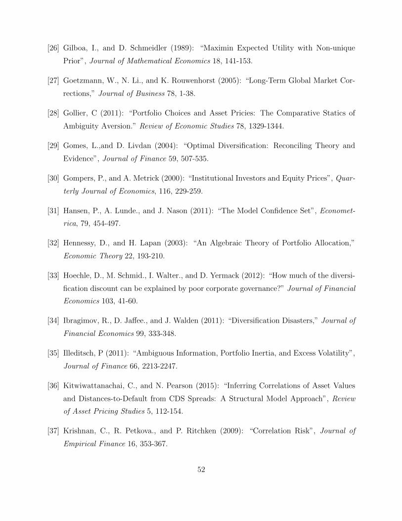
[26] Gilboa, I., and D. Schmeidler (1989): “Maximin Expected Utility with Non-unique
Prior”, Journal of Mathematical Economics 18, 141-153.
[27] Goetzmann, W., N. Li., and K. Rouwenhorst (2005): “Long-Term Global Market Cor-
rections,” Journal of Business 78, 1-38.
[28] Gollier, C (2011): “Portfolio Choices and Asset Pricies: The Comparative Statics of
Ambiguity Aversion.” Review of Economic Studies 78, 1329-1344.
[29] Gomes, L.,and D. Livdan (2004): “Optimal Diversification: Reconciling Theory and
Evidence”, Journal of Finance 59, 507-535.
[30] Gompers, P., and A. Metrick (2000): “Institutional Investors and Equity Prices”, Quar-
terly Journal of Economics, 116, 229-259.
[31] Hansen, P., A. Lunde., and J. Nason (2011): “The Model Confidence Set”, Economet-
rica, 79, 454-497.
[32] Hennessy, D., and H. Lapan (2003): “An Algebraic Theory of Portfolio Allocation,”
Economic Theory 22, 193-210.
[33] Hoechle, D., M. Schmid., I. Walter., and D. Yermack (2012): “How much of the diversi-
fication discount can be explained by poor corporate governance?” Journal of Financial
Economics 103, 41-60.
[34] Ibragimov, R., D. Jaffee., and J. Walden (2011): “Diversification Disasters,” Journal of
Financial Economics 99, 333-348.
[35] Illeditsch, P (2011): “Ambiguous Information, Portfolio Inertia, and Excess Volatility”,
Journal of Finance 66, 2213-2247.
[36] Kitwiwattanachai, C., and N. Pearson (2015): “Inferring Correlations of Asset Values
and Distances-to-Default from CDS Spreads: A Structural Model Approach”, Review
of Asset Pricing Studies 5, 112-154.
[37] Krishnan, C., R. Petkova., and P. Ritchken (2009): “Correlation Risk”, Journal of
Empirical Finance 16, 353-367.
52

[38] Ledoit, O., P. Santa-Clara., and M. Wolf (2003): “Flexible Multivariate GARCH Mod-
eling with an Application to International Stock Markets,” Review of Economics and
Statistics 85, 735-747.
[39] Longin, F., and B. Solnik (2001): “Extreme Correlation of International Equity Mar-
kets,” Journal of Finance 56, 649-676.
[40] Markowitz, H (1952): “Portfolio Selection,” Journal of Finance 7, 77-91.
[41] Mankiw, G., and S. Zeldes (1991): “The Consumption of Stockholders and Non-
stockholders,” Journal of Financial Economics 29, 97-111.
[42] Marshall, A., and I. Olkin (1979): Inequalities: Theory of Majorization and its Appli-
cations, Academic Press, New York.
[43] McNeil, A., R. Frey., and P. Embrechts (2015): Quantitative Risk Management: Con-
cepts, Techniques and Tools, Princeton University Press.
[44] Milgrom, P., and R. Weber (1982): “A Theory of Auction and Competitive Bidding,”
Econometrica 50, 1089-1122.
[45] Mitton, T., and K. Vorkink (2007): “Equilibrium Underdiversification and the Prefer-
ence for Skewness”, Review of Financial Studies 20, 1255-1288.
[46] Moskowitz, T (2003): “An Analysis of Covariance Risk and Pricing Anomalies,” Review
of Financial Studies 16, 417-457.
[47] Pindyck, R., and J. Rotemberg (1993): “The Comovement of Stock Prices,” Quarterly
Journal of Economics 108, 1073-1104.
[48] Rajan, R., Servases, H., and L. Zingales (2000): “The cost of diversity: The diversifi-
cation discount and inefficient investment,” Journal of Finance 60, 35-80.
[49] Routledge, B., and S. Zin (2014): “Generalized Disappointment Aversion and Asset
Prices,” Journal of Finance 65, 1303-1332.
[50] Samuelson, P (1967): “General Proof that Diversification Pays,” Journal of Financial
and Quantitative Analysis 2, 1-13.
53

[51] Simsek, A (2013): “Speculation and Risk Sharing with New Financial Assets,” Quarterly
Journal of Econimics, 1365-1396.
[52] Sion, M (1958): “On General Minimax Theorems,” Pacific Journal of Mathematics 8,
171-176.
[53] Solnik, B., and J. Roulet (2000): “Dispersion as Cross-Sectional Collelation”, Financial
Analyst Journal 56, 54-61.
[54] Strassen, V (1965): “The Existence of Probability Measures with Given Marginals,”
Annals of Mathematical Statistics, 36 (2), 423-439.
[55] Tola, V., F. Lillo., M. Gallegati., and R. Mantegna (2008): “Cluster Analysis for Port-
folio Optimization,” Journal of Dynamic and Control 32, 235-258.
[56] Towensend, R (1994): “Risk and Insurance in Village India,” Econometrica 62, 539-591.
[57] Uppal, R., and T. Wang (2003): “Model Misspecification and Underdiversification”,
Journal of Finance 58, 2465-2486.
[58] Van Nieuwerburgh, S., L. Veldkamp (2010): “Information Acquisition and Portfolio
Under-Diversification,” Review of Economic Studies 77, 779-805.
[59] Veklkamp, L (2006) : “Information Markets and the Comovement of Asset Prices,”
Review of Economic Studies 73, 823-845.
[60] Villalonga, B (2004): “Diversification Discount or Premium? Evidence from the Busi-
ness Information Tracking Series,” Journal of Finance 59, 479-506.
[61] Vissing-Jorgensen, A (2002): “Limited Asset Market Participation and the Elasticity
of Intertemporal Substitution,” Journal of Political Economy 110, 825-853.
[62] Whitt, W (1976): “Bivariate Distributions with Given Marginals,” Annals of Statistics,
4 (6), 1280-1289.
54
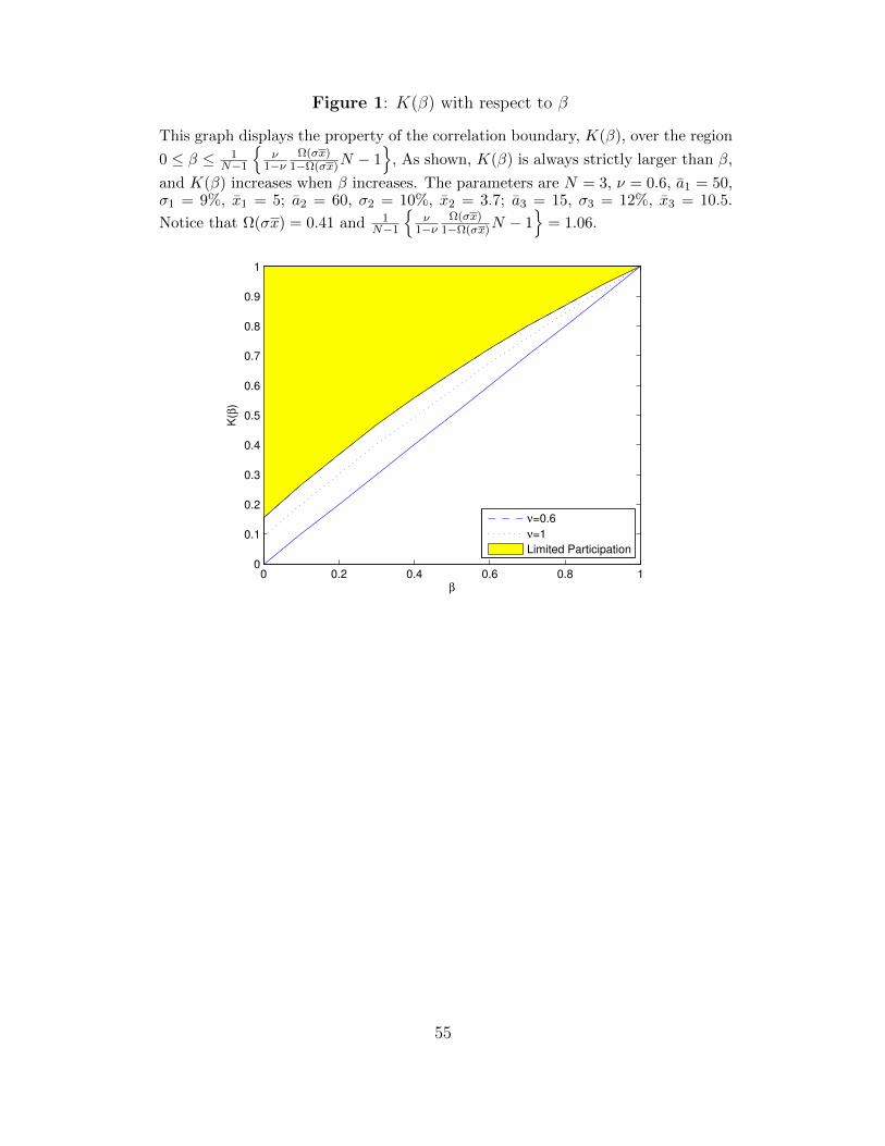
Figure 1: K(β) with respect to β
This graph displays the property of the correlation boundary, K(β), over the region
0 ≤ β ≤ 1N−1
ν
1−νΩ(σx)
1−Ω(σx)N − 1
, As shown, K(β) is always strictly larger than β,
and K(β) increases when β increases. The parameters are N = 3, ν = 0.6, a1 = 50,σ1 = 9%, x1 = 5; a2 = 60, σ2 = 10%, x2 = 3.7; a3 = 15, σ3 = 12%, x3 = 10.5.
Notice that Ω(σx) = 0.41 and 1N−1
ν
1−νΩ(σx)
1−Ω(σx)N − 1
= 1.06.
0 0.2 0.4 0.6 0.8 10
0.1
0.2
0.3
0.4
0.5
0.6
0.7
0.8
0.9
1
β
K(β
)
ν=0.6
ν=1
Limited Participation
55
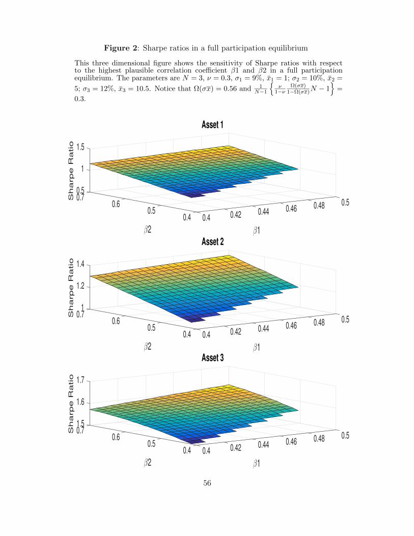
Figure 2: Sharpe ratios in a full participation equilibrium
This three dimensional figure shows the sensitivity of Sharpe ratios with respectto the highest plausible correlation coefficient β1 and β2 in a full participationequilibrium. The parameters are N = 3, ν = 0.3, σ1 = 9%, x1 = 1; σ2 = 10%, x2 =
5; σ3 = 12%, x3 = 10.5. Notice that Ω(σx) = 0.56 and 1N−1
ν
1−νΩ(σx)
1−Ω(σx)N − 1
=
0.3.
0.50.7
0.5
1
Sharpe R
atio
0.6 0.48
Asset 1
β2
0.46
β1
1.5
0.5 0.440.420.4 0.4
10.7
0.5
1.2
Sharpe R
atio
0.6 0.48
Asset 2
β2
0.46
β1
1.4
0.5 0.440.420.4 0.4
1.50.7
0.5
1.6
Sharpe R
atio
0.6 0.48
Asset 3
β2
0.46
β1
1.7
0.5 0.440.420.4 0.4
56
Figure 3: Dispersion of Sharpe Ratios
This three dimensional figure plots the dispersion, Ω(s), of Sharpe ratios in equi-librium A. As shown the dispersion decreases with increasing of β1 and β2, of so-phisticated and naive respectively. The same decreasing property of the disper-sion in the homogeneous environment and in Equilibrium B are reported in Table3 and Table 4. The parameters in this figure are N = 3, ν = 0.3, σ1 = 9%,x1 = 1; σ2 = 10%, x2 = 5; σ3 = 12%, x3 = 10.5. Notice that Ω(σs) = 0.56 and
1N−1
ν
1−νΩ(σx)
1−Ω(σx)N − 1
= 0.3.
0.08
0.7
0.1
0.65
0.12
0.5
Θ
0.6
0.14
0.48
Dispersion of Sharpe Ratios
β2
0.55
0.16
0.46
β1
0.18
0.50.44
0.45 0.42
0.4 0.4
57

Figure 4: Optimal Holdings of Agents
This figure reports the optimal holdings of the sophisticated and naive agent onhigh quality and low quality asset respectively. The parameters in this figure areN = 3, ν = 0.3, σ1 = 9%, x1 = 1; σ2 = 10%, x2 = 5; σ3 = 12%, x3 = 10.5. Notice
that Ω(σx) = 0.56 and 1N−1
ν
1−νΩ(σx)
1−Ω(σx)N − 1
= 0.3. σ1x1L = 0.048 < 1
N ,σ1x1L =
0.8582 > 1N .
1
1.5
0.7
2
0.65
2.5
0.5
3
optim
al positio
n
0.6
3.5
0.48
Sophisticated Agent Holdings on Asset 1
4
β2
0.55
4.5
0.46
β1
5
0.5 0.440.45 0.42
0.4 0.4
-0.8
-0.6
0.7
-0.4
-0.2
0.65
0
0.5
0.2
optim
al positio
n
0.6
0.4
0.48
Naive Agent Holdings on Asset 1
β2
0.6
0.55
0.8
0.46
β1
1
0.5 0.440.45 0.42
0.4 0.4
9.2
0.7
9.4
9.6
0.65
9.8
0.5
10
optim
al positio
n
0.60.48
10.2
Sophisticated Agent Holdings on Asset 3
β2
0.55
10.4
0.46
β1
10.6
0.5 0.440.45 0.42
0.4 0.4
10.5
0.7
10.6
0.65
10.7
0.5
optim
al positio
n
0.6
10.8
0.48
Naive Agent Holdings on Asset 3
β2
10.9
0.550.46
β1
11
0.5 0.440.45 0.42
0.4 0.458
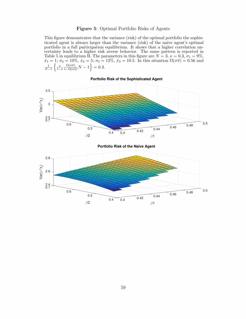
Figure 5: Optimal Portfolio Risks of Agents
This figure demonstrates that the variance (risk) of the optimal portfolio the sophis-ticated agent is always larger than the variance (risk) of the naive agent’s optimalportfolio in a full participation equilibrium. It shows that a higher correlation un-certainty leads to a higher risk averse behavior. The same pattern is reported inTable 5 in equilibrium B. The parameters in this figure are N = 3, ν = 0.3, σ1 = 9%,x1 = 1; σ2 = 10%, x2 = 5; σ3 = 12%, x3 = 10.5. In this situation Ω(σx) = 0.56 and
1N−1
ν
1−νΩ(σx)
1−Ω(σx)N − 1
= 0.3.
2.50.7
0.5
3
Va
r(σ
*xi)
0.6 0.48
Portfolio Risk of the Sophisticated Agent
β2
0.46
β1
3.5
0.5 0.440.42
0.4 0.4
2.40.7
0.5
2.6
Va
r(σ
*xi)
0.6 0.48
Portfolio Risk of the Naive Agent
β2
0.46
β1
2.8
0.5 0.440.42
0.4 0.4
59

Figure 6: Dispersion of Optimal Portfolios of Agents
This figure demonstrates the dispersion of the optimal portfolio the sophisticatedand naive agent respectively in a full participation equilibrium. Clearly, the disper-sion of the sophisticated agent’s optimal portfolio is smaller than the dispersion ofthe naive agent’s optimal portfolio for all possible values of β1 and β2. The samepattern is reported in Table 3 in a limited participation equilibrium. The parametersin this figure are N = 3, ν = 0.3, σ1 = 9%, x1 = 1; σ2 = 10%, x2 = 5; σ3 = 12%,
x3 = 10.5. Note that Ω(σx) = 0.56 and 1N−1
ν
1−νΩ(σx)
1−Ω(σx)N − 1
= 0.3.
0.20.7
0.5
0.4
Dis
pe
rsio
n
0.6 0.48
Dispersion of Sophisticated Agent
β2
0.46
β1
0.6
0.5 0.440.42
0.4 0.4
0.50.7
0.6
0.5
Dis
pe
rsio
n
0.6
0.7
0.48
Dispersion of Naive Agent
β2
0.46
β1
0.8
0.5 0.440.42
0.4 0.4
60
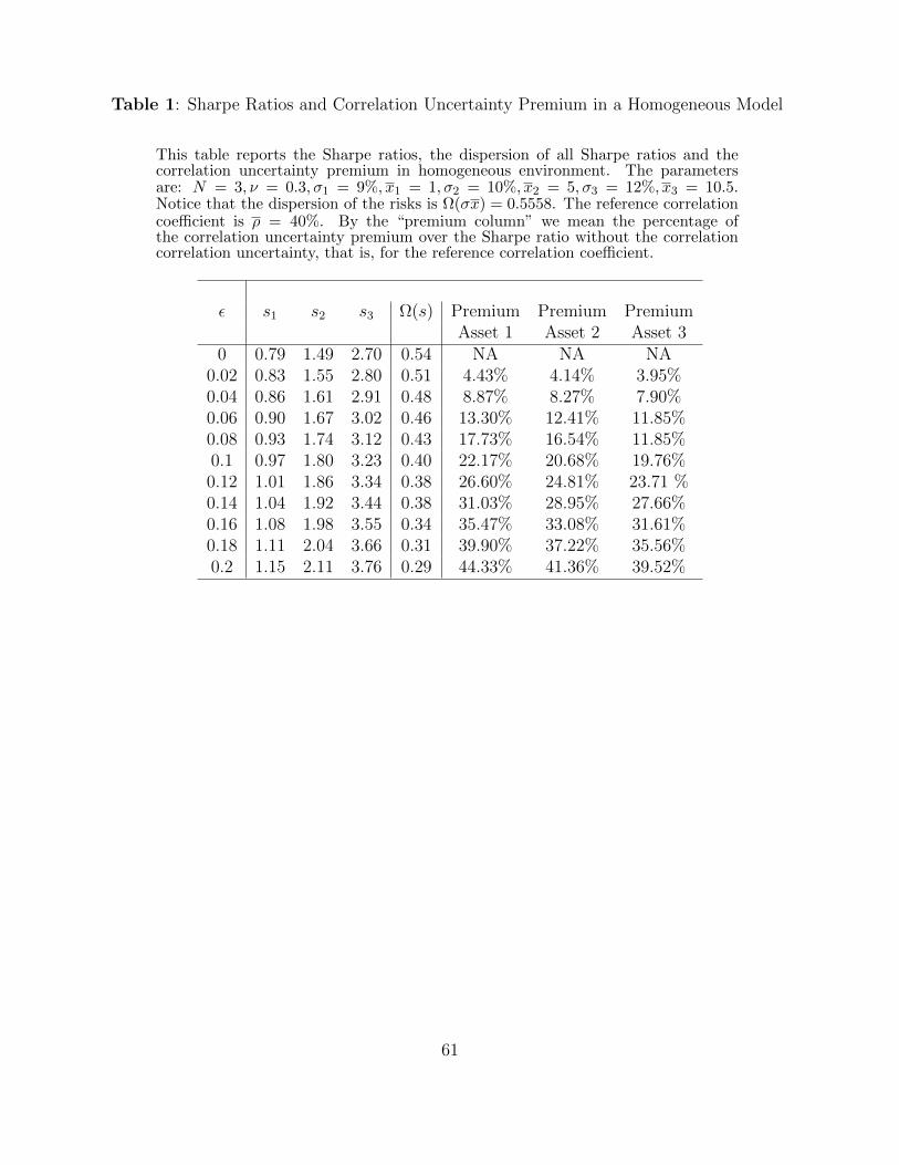
Table 1: Sharpe Ratios and Correlation Uncertainty Premium in a Homogeneous Model
This table reports the Sharpe ratios, the dispersion of all Sharpe ratios and thecorrelation uncertainty premium in homogeneous environment. The parametersare: N = 3, ν = 0.3, σ1 = 9%, x1 = 1, σ2 = 10%, x2 = 5, σ3 = 12%, x3 = 10.5.Notice that the dispersion of the risks is Ω(σx) = 0.5558. The reference correlationcoefficient is ρ = 40%. By the “premium column” we mean the percentage ofthe correlation uncertainty premium over the Sharpe ratio without the correlationcorrelation uncertainty, that is, for the reference correlation coefficient.
ε s1 s2 s3 Ω(s) Premium Premium PremiumAsset 1 Asset 2 Asset 3
0 0.79 1.49 2.70 0.54 NA NA NA0.02 0.83 1.55 2.80 0.51 4.43% 4.14% 3.95%0.04 0.86 1.61 2.91 0.48 8.87% 8.27% 7.90%0.06 0.90 1.67 3.02 0.46 13.30% 12.41% 11.85%0.08 0.93 1.74 3.12 0.43 17.73% 16.54% 11.85%0.1 0.97 1.80 3.23 0.40 22.17% 20.68% 19.76%0.12 1.01 1.86 3.34 0.38 26.60% 24.81% 23.71 %0.14 1.04 1.92 3.44 0.38 31.03% 28.95% 27.66%0.16 1.08 1.98 3.55 0.34 35.47% 33.08% 31.61%0.18 1.11 2.04 3.66 0.31 39.90% 37.22% 35.56%0.2 1.15 2.11 3.76 0.29 44.33% 41.36% 39.52%
61

Table 2: Sharpe ratios in a limited participation equilibrium
This table reports all Sharpe ratios in a limited participation equilibrium includingthe Sharpe ratios, the dispersion of all Sharpe ratios, the agent’s optimal positionand the corresponding dispersion of the optimal portfolio. The parameters are:N = 3, ν = 0.6, σ1 = 2%, x1 = 0.5, σ = 8%, x2 = 3, σ3 = 12%, x3 = 10.5. Notice thatthe dispersion of the risks is Ω(σx) = 0.7631. The reference correlation coefficientis ρ = 40%.
β1 K(β1) s1 s2 s3 S s1/S s2/S s3/S Ω(s)0.400 0.557 0.70 0.82 1.36 2.89 0.244 0.285 0.471 0.2100.405 0.561 0.71 0.83 1.36 2.90 0.245 0.286 0.469 0.2070.410 0.566 0.72 0.84 1.36 2.92 0.246 0.287 0.467 0.2040.415 0.570 0.73 0.84 1.36 2.93 0.247 0.287 0.465 0.2010.420 0.575 0.73 0.85 1.37 2.95 0.249 0.288 0.463 0.1980.425 0.579 0.74 0.86 1.37 2.96 0.250 0.289 0.461 0.1950.430 0.583 0.75 0.86 1.37 2.98 0.251 0.289 0.460 0.1920.435 0.588 0.75 0.87 1.37 2.99 0.252 0.290 0.458 0.1900.440 0.592 0.76 0.87 1.37 3.01 0.253 0.291 0.456 0.1870.445 0.596 0.77 0.88 1.37 3.02 0.255 0.291 0.454 0.1840.450 0.601 0.78 0.89 1.37 3.04 0.256 0.292 0.452 0.1810.455 0.605 0.78 0.89 1.37 3.05 0.257 0.292 0.452 0.1790.460 0.609 0.79 0.90 1.38 3.06 0.258 0.293 0.449 0.1760.465 0.613 0.80 0.90 1.38 3.08 0.259 0.294 0.447 0.1740.470 0.618 0.80 0.91 1.38 3.09 0.260 0.294 0.446 0.1710.475 0.622 0.81 0.92 1.38 3.11 0.261 0.295 0.444 0.1690.480 0.626 0.82 0.92 1.38 3.12 0.262 0.295 0.442 0.1660.485 0.630 0.83 0.93 1.38 3.14 0.263 0.296 0.441 0.1640.490 0.635 0.83 0.93 1.38 3.15 0.264 0.297 0.439 0.1610.495 0.639 0.84 0.94 1.38 3.16 0.265 0.297 0.438 0.1590.500 0.643 0.85 0.95 1.39 3.18 0.266 0.298 0.436 0.156
62
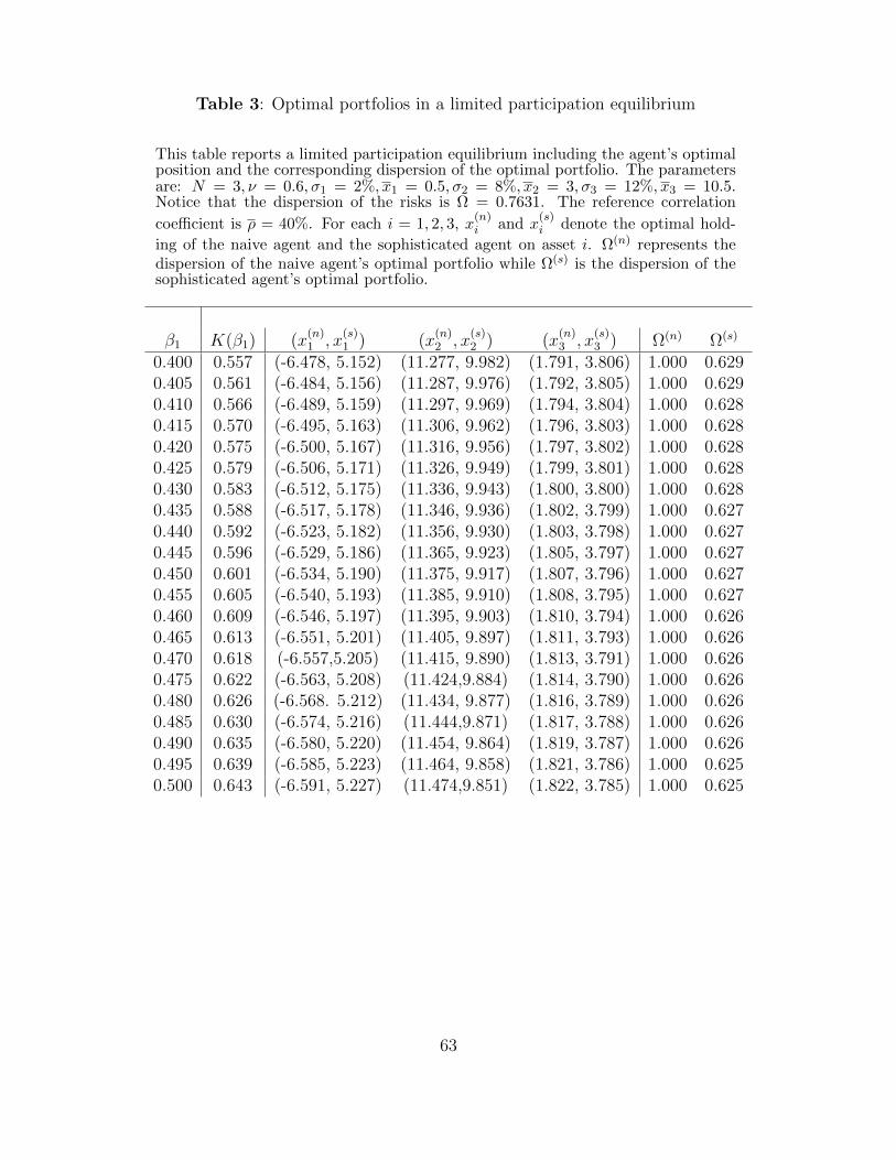
Table 3: Optimal portfolios in a limited participation equilibrium
This table reports a limited participation equilibrium including the agent’s optimalposition and the corresponding dispersion of the optimal portfolio. The parametersare: N = 3, ν = 0.6, σ1 = 2%, x1 = 0.5, σ2 = 8%, x2 = 3, σ3 = 12%, x3 = 10.5.Notice that the dispersion of the risks is Ω = 0.7631. The reference correlation
coefficient is ρ = 40%. For each i = 1, 2, 3, x(n)i and x
(s)i denote the optimal hold-
ing of the naive agent and the sophisticated agent on asset i. Ω(n) represents thedispersion of the naive agent’s optimal portfolio while Ω(s) is the dispersion of thesophisticated agent’s optimal portfolio.
β1 K(β1) (x(n)1 , x
(s)1 ) (x
(n)2 , x
(s)2 ) (x
(n)3 , x
(s)3 ) Ω(n) Ω(s)
0.400 0.557 (-6.478, 5.152) (11.277, 9.982) (1.791, 3.806) 1.000 0.6290.405 0.561 (-6.484, 5.156) (11.287, 9.976) (1.792, 3.805) 1.000 0.6290.410 0.566 (-6.489, 5.159) (11.297, 9.969) (1.794, 3.804) 1.000 0.6280.415 0.570 (-6.495, 5.163) (11.306, 9.962) (1.796, 3.803) 1.000 0.6280.420 0.575 (-6.500, 5.167) (11.316, 9.956) (1.797, 3.802) 1.000 0.6280.425 0.579 (-6.506, 5.171) (11.326, 9.949) (1.799, 3.801) 1.000 0.6280.430 0.583 (-6.512, 5.175) (11.336, 9.943) (1.800, 3.800) 1.000 0.6280.435 0.588 (-6.517, 5.178) (11.346, 9.936) (1.802, 3.799) 1.000 0.6270.440 0.592 (-6.523, 5.182) (11.356, 9.930) (1.803, 3.798) 1.000 0.6270.445 0.596 (-6.529, 5.186) (11.365, 9.923) (1.805, 3.797) 1.000 0.6270.450 0.601 (-6.534, 5.190) (11.375, 9.917) (1.807, 3.796) 1.000 0.6270.455 0.605 (-6.540, 5.193) (11.385, 9.910) (1.808, 3.795) 1.000 0.6270.460 0.609 (-6.546, 5.197) (11.395, 9.903) (1.810, 3.794) 1.000 0.6260.465 0.613 (-6.551, 5.201) (11.405, 9.897) (1.811, 3.793) 1.000 0.6260.470 0.618 (-6.557,5.205) (11.415, 9.890) (1.813, 3.791) 1.000 0.6260.475 0.622 (-6.563, 5.208) (11.424,9.884) (1.814, 3.790) 1.000 0.6260.480 0.626 (-6.568. 5.212) (11.434, 9.877) (1.816, 3.789) 1.000 0.6260.485 0.630 (-6.574, 5.216) (11.444,9.871) (1.817, 3.788) 1.000 0.6260.490 0.635 (-6.580, 5.220) (11.454, 9.864) (1.819, 3.787) 1.000 0.6260.495 0.639 (-6.585, 5.223) (11.464, 9.858) (1.821, 3.786) 1.000 0.6250.500 0.643 (-6.591, 5.227) (11.474,9.851) (1.822, 3.785) 1.000 0.625
63
Top Related