


Languages
Pages
Legal


Telemark University College
Department of Electrical Engineering, Information Technology and Cybernetics
Faculty of Technology, Postboks 203, Kjølnes ring 56, N-3901 Porsgrunn, Norway. Tel: +47 35 57 50 00 Fax: +47 35 57 54 01
→ Solutions
Control and Simulation in
LabVIEW HANS-PETTER HALVORSEN, 2011.08.11

ii
Table of Contents
Table of Contents .....................................................................................................................................ii
1 Differential Equations and Block Diagrams .................................................................................... 3
1.1 1. Order systems ...................................................................................................................... 3
1.2 2. Order systems ...................................................................................................................... 4
1.3 State space models .................................................................................................................. 5
2 Simulation in LabVIEW .................................................................................................................... 9
3 PID Control in LabVIEW ................................................................................................................ 15
4 Additional Tasks ............................................................................................................................ 18
5 PID Control on real process .......................................................................................................... 26
3
1 Differential Equations and
Block Diagrams
1.1 1. Order systems
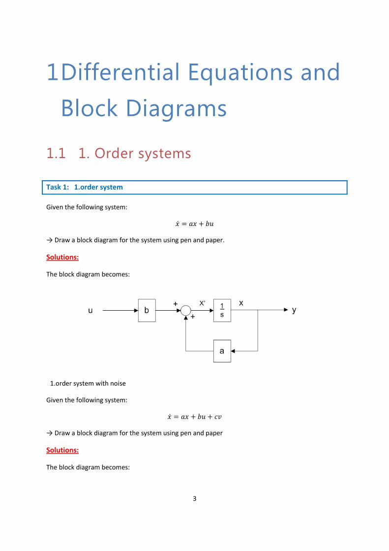
Task 1: 1.order system
Given the following system:
→ Draw a block diagram for the system using pen and paper.
Solutions:
The block diagram becomes:
1.order system with noise
Given the following system:
→ Draw a block diagram for the system using pen and paper
Solutions:
The block diagram becomes:

4 Differential Equations and Block Diagrams
Lab Work: Control and Simulation in LabVIEW - Solutions
[End of Task]
1.2 2. Order systems
Task 2: 2.order system
Given the following system:
→ Draw a block diagram for the system using pen and paper.
is the position
is the speed
is the acceleration
F is the Force (control signal, u)
d and k are constants
[End of Task]
Solutions:
We do the following:

5 Differential Equations and Block Diagrams
Lab Work: Control and Simulation in LabVIEW - Solutions
[ ]
The block diagram becomes:
You may also use this notation:
1.3 State space models
Task 3: State Space model
Given the following system:

6 Differential Equations and Block Diagrams
Lab Work: Control and Simulation in LabVIEW - Solutions
→ Draw a block diagram for the system using pen and paper
Solutions:
The block diagram becomes:
1
sa2
1
s
b
a1
c
y
u - --
x1x2
Given the following state-space model:
[
] [
] [
] [
]
→ Draw the block diagram for this model using pen and paper.
Solutions:
The differential equations becomes:
The block diagram becomes:

7 Differential Equations and Block Diagrams
Lab Work: Control and Simulation in LabVIEW - Solutions
1
s2
1
s
u
-
x2x1
2
6
Given the following system:
→ Find the state-space model on the form:
Draw the block diagram for this simplified model using pen and paper
Solutions:
We get the following state-space model:
[
] [
] [
] [
]
[ ] [
]
Block diagram for
becomes:

8 Differential Equations and Block Diagrams
Lab Work: Control and Simulation in LabVIEW - Solutions
[End of Task]

9
2 Simulation in LabVIEW
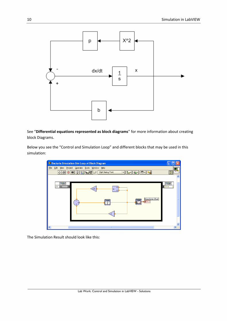
Task 4: Bacteria Population
In this task we will use LabVIEW and the LabVIEW Control Design and Simulation Module to simulate
a simple model of a bacteria population in a jar.
The model is as follows:
birth rate=bx
death rate = px2
Then the total rate of change of bacteria population is:
Set b=1/hour and p=0.5 bacteria-hour
We will simulate the number of bacteria in the jar after 1 hour, assuming that initially there are 100
bacteria present.
You should follow these steps:
1. Draw Block Diagram using “pen and paper”.
2. Start LabVIEW and use the Control and Simulation Loop from Control Design and
Simulation Palette in LabVIEW
3. Drag in the necessary Blocks from the palette.
4. Use the “Connection Wire” from the Tools palette and draw the necessary wires.
5. Configure Simulation Parameters (right-click on the Control and Simulation Loop border)
6. Start the Simulation. The Simulation result should be present in a plot.
[End of Task]
Solutions:
The Block Diagram becomes:
10 Simulation in LabVIEW
Lab Work: Control and Simulation in LabVIEW - Solutions
See “Differential equations represented as block diagrams” for more information about creating
block Diagrams.
Below you see the “Control and Simulation Loop” and different blocks that may be used in this
simulation:
The Simulation Result should look like this:

11 Simulation in LabVIEW
Lab Work: Control and Simulation in LabVIEW - Solutions
Task 5: Simulation of a “spring-mass damper” system in LabVIEW
Use “LabVIEW Control Design and Simulation Module” and the “Control and Simulation
Loop” in order to create a simulation of a spring-mass damper system.
The differential equation for the system is as follows:

12 Simulation in LabVIEW
Lab Work: Control and Simulation in LabVIEW - Solutions
Where.
F is an external force applied to the system
c is the damping constant of the spring
k is the stiffness of the spring
m is a mass
x is the position of the mass
is the first derivative of the position, which equals the velocity of the mass
is the second derivative of the position, which equals the acceleration of the mass
Note! Draw a block diagram of the system using pen and paper before you implement the system in
LabVIEW.
In the simulations you may set
Then try to set and see the difference.
[End of Task]
Solutions:
See the video “Simulation Palette Overview” by Finn Haugen for a step-by-step instructions or read
the Tutorial “Control and Simulation in LabVIEW” for step-by-step instructions.
Block Diagram:

13 Simulation in LabVIEW
Lab Work: Control and Simulation in LabVIEW - Solutions
You may also use this notation:
LabVIEW:
Block Diagram:
Front Panel:

14 Simulation in LabVIEW
Lab Work: Control and Simulation in LabVIEW - Solutions

15
3 PID Control in LabVIEW
Task 6: Built-in PID Controller in LabVIEW
In this task you will use the example “General PID Simulator.vi” as a base for your simulation. Use
the “NI Example Finder” (Help → Find Examples…) in order to find the VI in LabVIEW.
Run the example and so how it is implemented and how it works.
Make changes to the program (make sure to save it with another name) and use the “PID
Advance.vi” function instead.
Note that and is in minutes, while it’s normal to use seconds as the unit for these
parameters. So it is recommended that you do like this in your code:

16 PID Control in LabVIEW
16
Try with different values for , and and see what happens.
[End of Task]
Solutions:
Front Panel:
PID Parameters:

17 PID Control in LabVIEW
17
Block Diagram:

18
4 Additional Tasks
Task 7: Simulation Loop
Given the following (nonlinear) system of a liquid tank:
√
where is the input (control value), is the output (level), is the valve outflow parameter,
and is the pump inflow parameter.
Find proper values for , and . Apply a Step signal for
→ Create an application where you use “LabVIEW Control Design and Simulation Module” and the
“Control and Simulation Loop” in order to simulate the system. Here you will use the simulation
blocks from the Simulation palette in LabVIEW to create a continuous model.
Plot the results.
[End of Task]
Solutions:
Block Diagram:
Front Panel:

19 Additional Tasks
19
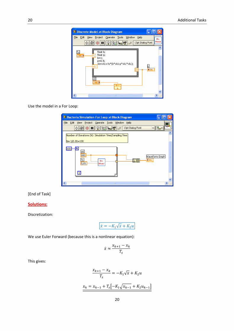
Task 8: Discretization
Given the following (nonlinear) system of a liquid tank:
√
→ Create a new application in LabVIEW where you Simulate the model using a Formula Node to
implement the discrete model.
Use one of Eulers Discretization methods in order to create a discrete model of the system. Which of
Eulers methods did you use? Why?
Use a While Loop or a For Loop and select a proper time-step for the simulation. Use the same
settings and values as in the previous case.
→ Compare the results from the 2 different methods used above. Do you get the same results?
Example:
Implementing the model as a SubVI using the Formula Node:
20 Additional Tasks
20
Use the model in a For Loop:
[End of Task]
Solutions:
Discretization:
√
We use Euler Forward (because this is a nonlinear equation):
This gives:
√
[ √ ]

21 Additional Tasks
21
Block Diagram:
Front Panel:
Task 9: Simulation and Control in LabVIEW
Control the system created above using a discrete PI controller that you create yourself.
A PI controller may be written:
∫
22 Additional Tasks
22
Where u is the controller output and e is the control error:
Compare the results from the previous task.
[End of Task]
Solutions:
Discretization:
Given:

23 Additional Tasks
23

24 Additional Tasks
24
Discrete PI Controller in LabVIEW (implemented in SubVI using a Formula Node):
Block Diagram:
Front Panel:

25 Additional Tasks
25
Test of the PI Controller:
Front Panel:
Block Diagram:

26
5 PID Control on real
process
Create a PID Control system for a real process.
Below we see the Lab Equipment available for this assignment:
Level Tank Air Heater
Documents of how to use the Level Tank/Air Heater and the USB-6008 DAQ device is
available from http://home.hit.no/~hansha.
Level Tank: http://home.hit.no/~hansha/?equipment=leveltank
Air Heater: http://home.hit.no/~hansha/?equipment=airheater
USB-6008: http://home.hit.no/~hansha/?equipment=usb6008
Find proper PID parameters. Use, e.g., Skogestad’s method in order to find PID parameters.
Skogestad’s method:
In this task we assume the following process:

27 PID Control on real process
27
You need to apply a step on the input (u) and then observe the response and the output, as shown
below:
Here are the Skogestad’s formulas for finding the PID parameters:
The Skogestad’s formulas for this system are:
[ ]
Air Heater: Set sec and .
Water Tank: Set sec and .
For more details about the Skogestads method, please read this article: “Model-based PID tuning
with Skogestad’s method”.
[End of Task]

28 PID Control on real process
28
Solutions:
Using Skogestads method on the Air Heater:
In this task we can set sec and .
We assume the following transfer function:
The Skogestad’s formulas for this system are:
[ ]
From a previous task we have:
The control signal is a step with at .
From the plot above we can find:
Gain:

29 PID Control on real process
29
With we get:
Time-delay:
Time constant:
Comments: T is too small?? Have the response above reached steady-state?
This gives the following PID parameters from Skogestad’s formulas:
[ ] [ ]
Trying out the PID parameters found above:
Trying other PID Parameters:

30 PID Control on real process
30
Here are some values that worked fine for me from another assignment:
These PID parameters gave the following results:
These PID parameters gives a better result.
LabVIEW Program for Air Heater – Example II:
Block Diagram:

31 PID Control on real process
31
Front Panel:

Telemark University College
Faculty of Technology
Kjølnes Ring 56
N-3914 Porsgrunn, Norway
www.hit.no
Hans-Petter Halvorsen, M.Sc.
Telemark University College
Department of Electrical Engineering, Information Technology and Cybernetics
Phone: +47 3557 5158
E-mail: [email protected]
Blog: http://home.hit.no/~hansha/
Room: B-237a
Top Related