Computing Three-dimensional ConstrainedDelaunay Refinement Using the GPU

Zhenghai Chen and Tiow-Seng TanSchool of Computing

National University of Singapore

Singapore

{chenzh, tants}@comp.nus.edu.sg

Abstract—We propose the first GPU algorithm for the 3Dconstrained Delaunay refinement problem. For an input of apiecewise linear complex G and a constant B, it produces,by adding Steiner points, a constrained Delaunay triangulationconforming to G and containing tetrahedra mostly with radius-edge ratios smaller than B. Our implementation of the algorithmshows that it can be an order of magnitude faster than the bestCPU software while using similar quantities of Steiner points toproduce triangulations of comparable qualities. It thus reducesthe computing time of triangulation refinement from possibly anhour to a few seconds or minutes for possible use in interactiveapplications.

Index Terms—GPGPU, Computational Geometry, Mesh Re-finement, Finite Element Analysis

I. INTRODUCTION

Triangulations are used in various engineering and scientific

applications such as finite element methods, interpolation etc.

Such a triangulation, in general, is obtained from a so-called

piecewise linear complex (PLC) G containing a point set P ,

an edge set E (where each edge has endpoints in P ), and a

polygon set F (where each polygon has boundary edges in E)

[1]. Specifically, a triangulation T of G is a decomposition of

the convex hull of P into tetrahedra where the intersection

of any two tetrahedra is either empty, a vertex, an edge, or a

triangle of both tetrahedra. In addition, all vertices, edges and

polygons of G also appear in T as vertices, unions of edges,

and unions of triangles, respectively; we also say T conformsto G in this case. To ease our discussion, we call an edge in

E a segment, an edge in T which is also a part or whole of

some segment a subsegment, and a triangle in T which is also

a part or whole of some polygon in F a subface.

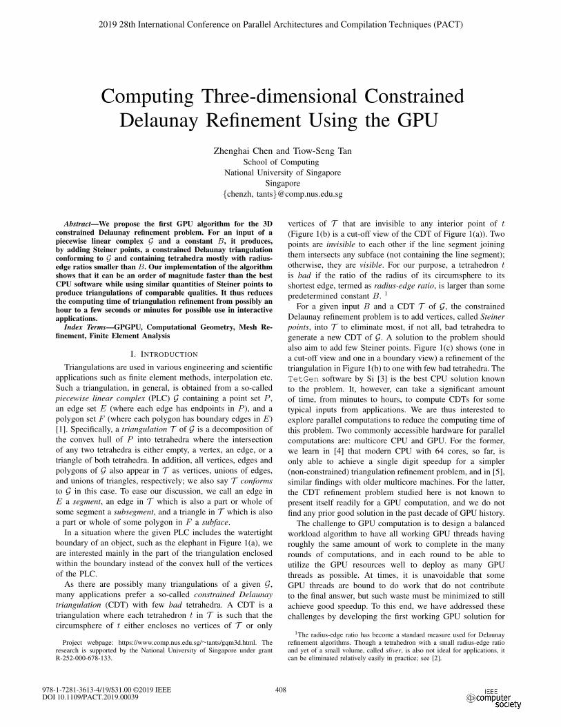
In a situation where the given PLC includes the watertight

boundary of an object, such as the elephant in Figure 1(a), we

are interested mainly in the part of the triangulation enclosed

within the boundary instead of the convex hull of the vertices

of the PLC.

As there are possibly many triangulations of a given G,

many applications prefer a so-called constrained Delaunaytriangulation (CDT) with few bad tetrahedra. A CDT is a

triangulation where each tetrahedron t in T is such that the

circumsphere of t either encloses no vertices of T or only

Project webpage: https://www.comp.nus.edu.sg/∼tants/gqm3d.html. Theresearch is supported by the National University of Singapore under grantR-252-000-678-133.

vertices of T that are invisible to any interior point of t(Figure 1(b) is a cut-off view of the CDT of Figure 1(a)). Two

points are invisible to each other if the line segment joining

them intersects any subface (not containing the line segment);

otherwise, they are visible. For our purpose, a tetrahedron tis bad if the ratio of the radius of its circumsphere to its

shortest edge, termed as radius-edge ratio, is larger than some

predetermined constant B. 1

For a given input B and a CDT T of G, the constrained

Delaunay refinement problem is to add vertices, called Steinerpoints, into T to eliminate most, if not all, bad tetrahedra to

generate a new CDT of G. A solution to the problem should

also aim to add few Steiner points. Figure 1(c) shows (one in

a cut-off view and one in a boundary view) a refinement of the

triangulation in Figure 1(b) to one with few bad tetrahedra. The

TetGen software by Si [3] is the best CPU solution known

to the problem. It, however, can take a significant amount

of time, from minutes to hours, to compute CDTs for some

typical inputs from applications. We are thus interested to

explore parallel computations to reduce the computing time of

this problem. Two commonly accessible hardware for parallel

computations are: multicore CPU and GPU. For the former,

we learn in [4] that modern CPU with 64 cores, so far, is

only able to achieve a single digit speedup for a simpler

(non-constrained) triangulation refinement problem, and in [5],

similar findings with older multicore machines. For the latter,

the CDT refinement problem studied here is not known to

present itself readily for a GPU computation, and we do not

find any prior good solution in the past decade of GPU history.

The challenge to GPU computation is to design a balanced

workload algorithm to have all working GPU threads having

roughly the same amount of work to complete in the many

rounds of computations, and in each round to be able to

utilize the GPU resources well to deploy as many GPU

threads as possible. At times, it is unavoidable that some

GPU threads are bound to do work that do not contribute

to the final answer, but such waste must be minimized to still

achieve good speedup. To this end, we have addressed these

challenges by developing the first working GPU solution for

1The radius-edge ratio has become a standard measure used for Delaunayrefinement algorithms. Though a tetrahedron with a small radius-edge ratioand yet of a small volume, called sliver, is also not ideal for applications, itcan be eliminated relatively easily in practice; see [2].

408

2019 28th International Conference on Parallel Architectures and Compilation Techniques (PACT)

978-1-7281-3613-4/19/$31.00 ©2019 IEEEDOI 10.1109/PACT.2019.00039

Fig. 1. gQM3D working on the PLC of an elephant.

the CDT refinement problem. Specifically, its contributions are

as follows:

(1) a GPU algorithm, gQM3D, and a CPU-GPU hybrid vari-

ant, gQM3D+, that solve the CDT refinement problem for

PLC with an order of magnitude speedup as compared to

the best CPU software, TetGen while still maintaining

similar output sizes and comparable qualities;

(2) at the algorithmic level, an efficient and effective parallel

GPU pipeline, InsertPoints, to concurrently insert

points to refine a triangulation, which can be useful to

solve other refinement problems; and

(3) at the data structure level, a tuple structure to keep track

of work in progress and result of work done to provide

good support for the extensive use of parallel prefix and

stream compaction in the GPU solution.

In this paper, we start the discussion with Section II which

reviews important previous work, and then Section III which

discusses the considerations and challenges of designing our

GPU solution, followed by Section IV which details the

proposed algorithms gQM3D and gQM3D+. Then, Section V

presents our experimental results in comparison with the best

CPU software, TetGen, and finally, Section VI concludes the

paper.

II. LITERATURE REVIEW

In 2D, Chew [6], [7] and Ruppert [8] proposed algorithms

that output triangulations whose triangles have good attributes

(such as no small angles) for an input of points and segments.

On the same problem, Chen et al. [9] developed a GPU

algorithm that unifies both Chew’s and Ruppert’s to achieve

good speedup of over an order of magnitude.

In 3D, Dey et al. [10] and Chew [11] generalized Chew’s

algorithm [7] to compute the Delaunay triangulation of a set of

input points without constraints. Both algorithms produce uni-

form triangulations that contain tetrahedra of roughly the same

size. However, they sometimes need many more tetrahedra

than necessary as they do not take advantage of using different

large size tetrahedra where possible. For an input of a constant

B and a PLC, Shewchuk [2] proposed a provably correct

Delaunay refinement algorithm. The algorithm is guaranteed

to terminate with a conforming Delaunay triangulation when

B > 2 and the PLC has no acute angles. However, this

approach may need to use a large number of Steiner points to

complete the computation.

An alternative approach is to first compute a CDT, as

discussed in Shewchuk [12] and Si [13], and then further refine

the CDT to one with few, if any, bad tetrahedra. This approach,

as implemented by Si [3] in TetGen, usually produces a

smaller triangulation than that of Shewchuk’s algorithm [2]

which generates the conforming Delaunay triangulation.

Oudot et al. [14] introduced a triangulation generation

algorithm for input domains bounded by smooth surfaces

while Cheng et al. [15] for piecewise smooth complexes. Both

algorithms, as implemented in CGAL [16], use the notion of

a restricted Delaunay triangulation to approximate the domain

boundary by a new boundary triangulation. Because of this

approximation, the output need not conform to the input

surface or complex. Building on top of CGAL, Hu et al.[17] proposed an algorithm called TetWild that converts a

triangle soup into a triangulation. This algorithm focuses on

robustness and is often slower than both TetGen and CGAL.

In parallel computation, Blandford et al. [18] proposed

a space-efficient Delaunay algorithm based on a concurrent

compressed data structure, while Foteinos and Chrisochoides

[5] presented one that offers fully dynamic parallel insertions

and removal of points, and Marot et al. [4] introduced a

scalable parallelization scheme that uses Moore’s curve for

space partitioning. All these are multicore CPU algorithms

working on point sets that do not handle the more complex

cases of PLCs. For PLC, Chernikov and Chrisochoides [19]

proposed an octree to partition the domain for triangulation to

discover work that can be scheduled to run concurrently on

multicore CPU. However, there are neither efficient scheduling

algorithm nor experimental results known that can achieve

good speedup. The latest known, with the use of multicore

CPU, for a refinement problem (on point sets only) is in [4].

It experimented with Intel Core i7-6700HQ 4-core and AMD

EPYC 64-core, but was only able to achieve a small single

digit speedup, a result that is far from being effective on refine-

ment in comparison to our approach of using (an inexpensive)

GPU that achieves an order of magnitude speedup.

III. EXPLORING GPU FOR REFINEMENT

The heart of refining a triangulation T is to add as many

Steiner points as needed to eliminate bad tetrahedra. As bad

tetrahedra possibly resulted from segments (or subsegments)

and polygons (or subfaces), from the input, that are on their

boundaries and are forced to appear in the output triangula-

409

tion, Steiner points are also needed to split subsegments and

subfaces into smaller ones. The center of the circumsphere of

a bad tetrahedron, the center of the circumcircle of a subface,

and the midpoint of a subsegment are points calculated as

splitting points and some of them will be inserted as Steiner

points of T . Whenever a splitting point p becomes a Steiner

point in T , those tetrahedra whose circumspheres enclose pand interior points visible to p have to be eliminated and be

replaced by tetrahedra incident to p.

It is obvious then that the use of GPU to do refinement

is to design a GPU-friendly algorithm to compute splitting

points and add them as Steiner points, as needed, concurrently

by thousands of GPU threads. This is to be repeated round

after round while maintaining T , a constrained Delaunay

triangulation, until either no more bad tetrahedra, in the best

case, or some unsplittable ones, that are futile to continue

processing, are left.

To be GPU-friendly, an algorithm launching concurrently

with thousands of GPU threads at each step would want

threads to have balanced workload and regularized work to

maximize the utilization of GPU capacity. This results in a

number of design considerations which are unique to GPU

parallel computation and do not exist in a sequential CPU

one. These considerations are discussed in the following

subsections with each addressed by our algorithm in the

corresponding subsection in Section IV.

A. Priorities of Splitting Points

It is natural to think of using one GPU thread to calculate

a splitting point, locate it within some tetrahedron of T , and

then add it as a Steiner point. However, any two Steiner points

inserted concurrently in the same round must be so-called

Delaunay independent, i.e., they must not form an edge (which

can be too short) in T , so as to avoid non-termination of the

algorithm. For a splitting point p, its Delaunay region [20] is

defined as the union of tetrahedra in T whose circumspheres

enclose p and whose interior points are visible to p. When two

splitting points are such that the intersection of their Delaunay

regions contain at most some vertices or edges of T , they are

indeed Delaunay independent. So, the goal is to design an

algorithm to allow the insertion of many, if not all, splitting

points with mutually disjoint Delaunay regions. Unavoidably,

the algorithm needs to prioritize among all splitting points to

retain a subset with mutually disjoint Delaunay regions for

concurrent insertions.

B. Supporting Data Structures

For computations on triangulations, the standard

tetrahedron-based data structure [21] supports stepping

(walking) from one element, either vertex, edge, face, or

tetrahedron, to any of its neighbor in constant time.2 With it, a

GPU thread can take linear time (to the number of tetrahedra

in the Delaunay region) to identify the Delaunay region for

2We adapt the usual practice used in [22] to have an infinite vertex toconnect to all boundary faces of the triangulation to form “ghost” tetrahedra,and to all boundaries of input polygons of F in G to form “ghost” subfaces.

a splitting point. However, Delaunay regions often come in

different sizes and thus the handling of each region by one

GPU thread would result in unbalanced workload among

thousands of concurrent GPU threads. In this way, the task for

a GPU thread to decide whether a Delaunay region overlaps

some others would not be a balanced workload computation

either. Moreover, this computation is needed for each splitting

point, regardless of whether it eventually becomes a Steiner

point, and thus on the whole undoubtedly taking away lots

of computing power of the GPU. Most of these computations

are verification in nature and do not contribute directly to

refining a triangulation as they are not needed in any CPU

algorithm. Therefore, such “inessential” computations in GPU

must be done efficiently to waste little computing time to pay

for identifying a large subset of splitting points with mutually

disjoint Delaunay regions for concurrent insertions. To this

end, using one GPU thread, supported with only the standard

tetrahedron-based data structure (as in the CPU algorithm),

to compute a Delaunay region is not a wise approach.

C. Cavity Growing

One idea to avoid wasting the computation of Delaunay

regions is to piggyback this to the actual insertion of a splitting

point as a Steiner point. That is, a splitting point p is pretended

to be a Steiner point of T and flipping is carried out to restore

the Delaunay property of T and in turn also identify the

Delaunay region of p. When flips of different splitting points

collide (i.e., their Delaunay regions are found to overlap), some

flips for one splitting point will be undone. Such a strategy

was employed successfully for the 2D problem [9]. It is,

however, unclear whether this can work for 3D problems since

flipping (to undo some earlier flips) is not known to be able

to reach all possible triangulations [23]. As a consequence, an

algorithm with mainly (parallel) flipping can be stuck at a state

where it does not know how to restore to some old state with

more flipping. Hence, the computation of Delaunay regions

has to be decoupled from the insertion of splitting points

with GPU threads. In order to compute a Delaunay region,

the next alternative is to systematically grow the so-called

cavity. Initially, the cavity of a splitting point p is the collection

of tetrahedra incident to or containing p. The cavity is then

grown by progressively adding tetrahedra, which have their

circumspheres enclosing p, incident to the boundary of the

current cavity. In other words, the cavity is a partial Delaunay

region growing towards a Delaunay region. Whichever the

approach may be, an algorithm has to employ concurrent GPU

threads with regularized work to grow cavities.

D. Cavity Shrinking

Because we work with the constrained Delaunay triangu-

lation, a Delaunay region of a splitting point p only includes

tetrahedra whose interiors are visible to p besides having pinside their circumspheres. As such, the growing of the cavity

of p should stop once it hits some subface that occludes the

visibility. Such stopping can shield away subsegments and

subfaces that are invisible but may prohibit the insertion of

410

p before their splittings. Hence, without knowing what have

been occluded, a decision to proceed to insert p may be

premature and can result in the need to remove p in subsequent

processing (which can be costly under a parallel setting;

see [5]). Considering this, we need to weigh the advantage

of saving some computation by growing the cavity without

considering the visibility against the disadvantage of shrinking

to amend the cavity to its Delaunay region.

E. Termination

All in all, any refinement algorithm must be mindful to

still terminate while adding many Steiner points concurrently.

In our algorithm, splitting points are computed and located in

tetrahedra, then they are filtered out in different stages to leave

behind only those that are Delaunay independent for insertions.

The filtering starts immediately after the splitting points are

located in tetrahedra where each tetrahedron can only house

one splitting point. Then, the growing of cavities is meant for

splitting points to gradually obtain their complete Delaunay

regions; those which cannot complete are filtered out. Before

shrinking the cavity of the splitting point of an element

e, this cavity is aborted if there are other subsegments or

subfaces which are supposed to be split before e because their

dimensions are lower than that of e. A final check is used to

ensure that the splitting points of completed Delaunay regions

are indeed Delaunay independent and that these splitting points

can be inserted as Steiner points to create new tetrahedra to

complete this round of concurrent point insertions.

IV. OUR PROPOSED ALGORITHM

Our proposed GPU algorithm is depicted in Algorithm 1 as

gQM3D. For an input PLC G, we can assume its CDT exists or

we use the approach in [24] to split its edges to guarantee so.

We thus discuss our algorithm with an input constant B and

a CDT T of G that has bad tetrahedra due for refinement. A

subsegment or subface e is so-called encroached when there

exists a point q, which is a vertex of T or a splitting point,

inside the diametric sphere of e. In this case, q is called an

encroaching point that encroaches upon e.

The algorithm gQM3D starts by recording encroached sub-

segments (Line 1 to 3), encroached subfaces (Line 4 to 6) and

bad tetrahedra (Line 7 to 9) in the input CDT for refinement.

Next, it refines encroached subsegments (Line 10, 25 and 32),

encroached subfaces (Line 11 and 33) and bad tetrahedra (Line

12) in this order iteratively until SplitBadTets terminates

with no more bad tetrahedra or only bad tetrahedra that

are unsplittable. In every iteration of repeat-until in these

routines, the elements, which are subsegments, subfaces and

bad tetrahedra, to be split or eliminated are collected into the

list M using stream compaction (Line 16, 22 and 29) and then

passed to the pipeline of InsertPoints (Line 18, 24 and

31), a concurrent point insertion routine (see Section IV-A).

As designed, gQM3D gives higher priority to the splitting

points of subsegments (lowest dimension) followed by those of

subfaces and finally those of bad tetrahedra (highest dimen-

sion). This is natural as lower dimension problems must be

Algorithm 1: gQM3DInput: CDT T of PLC G; constant BOutput: Quality Mesh T , which is also a CDT

// Recording elements for refinement1 for each subsegment s ∈ T in parallel do2 if the diametric sphere of s encloses any vertex of T

then3 Record s as encroached in T4 for each subface f ∈ T in parallel do5 if the diametric sphere of f encloses any vertex of T

then6 Record f as encroached in T7 for each tetrahedron t ∈ T in parallel do8 if the radius-edge ratio of t is larger than B then9 Record t as a bad tetrahedron in T

// Refinement steps10 SplitEncSubsegments(T , B)11 SplitEncSubfaces(T , B)12 SplitBadTets(T , B)13 End// Routine definitions

14 Procedure SplitEncSubsegments(T , B)15 repeat16 Collect all encroached subsegments into list M in

parallel17 if M �= ∅ then18 InsertPoints(T ,M,B)

19 until M = ∅20 Procedure SplitEncSubfaces(T , B)21 repeat22 Collect all encroached subfaces into list M in

parallel23 if M �= ∅ then24 InsertPoints(T ,M,B)25 SplitEncSubsegments(T , B)

26 until M = ∅27 Procedure SplitBadTets(T , B)28 repeat29 Collect all bad tetrahedra into list M in parallel30 if M �= ∅ then31 InsertPoints(T ,M,B)32 SplitEncSubsegments(T , B)33 SplitEncSubfaces(T , B)

34 until M = ∅

solved before higher dimension ones. On another matter, our

experiments show that gQM3D does not have any particular

advantage over the CPU approach for splitting encroached

subsegments and subfaces at Line 10 and 11. This is because

such splittings take many rounds of point insertions but each

does not have heavy workload to fill GPU capacity. This

low utilization of GPU capacity is also observed for Line 32

and 33 in SplitBadTets due to the fact that the number

of encroached subsegments and subfaces are generally small

after Line 10 and 11. As such, a CPU-GPU hybrid variant

called gQM3D+, shown in Algorithm 2, is developed from

gQM3D by making two adjustments: (1) it has Line 1 and

2 to split encroached subsegments and subfaces by TetGen

411

Algorithm 2: gQM3D+

Input: CDT T of PLC G; constant BOutput: Quality Mesh T , which is also a CDT

// Refinement steps on the CPU1 SplitEncSubsegments_CPU(T , B)2 SplitEncSubfaces_CPU(T , B)3 Copy T from CPU to GPU

// Refinement steps on the GPU4 Line 1 to 9 as in Algorithm 15 SplitBadElements(T , B)6 End// Routine definitions

7 Procedure SplitBadElements(T , B)8 repeat9 Collect all encroached subsegments, subfaces and

bad tetrahedra into list M in parallel10 if M �= ∅ then11 InsertPoints(T ,M,B)

12 until M = ∅

in CPU, which correspond to Line 10 and 11 of gQM3D,

respectively; and (2) it replaces SplitBadTets (Line 12) of

gQM3D by SplitBadElements (Line 5), which processes

all elements of different types in one single routine, and

still respects the priority of processing elements from lower

to higher dimensions. In this way, the leftover capacity of

GPU during the splitting of subsegments and subfaces can

be utilized to eliminate bad tetrahedra to gain good speedup.

Note that if the first adjustment is not employed, gQM3D+ can

remain as a pure GPU algorithm, like gQM3D.

A. Concurrent Point Insertions Pipeline

Both gQM3D and gQM3D+ rely on InsertPoints to

achieve high parallelism. It takes a set of elements, each an

encroached subsegment, encroached subface or bad tetrahe-

dron as input to decide a subset of these elements to be

split concurrently while ensuring termination of the algorithm.

For gQM3D, it processes a set of homogeneous elements of

either encroached subsegments, encroached subfaces or bad

tetrahedra, individually and not a mixture of them. On the

other hand, for gQM3D+, all the different types of elements

can be processed at the same time while still respecting higher

priorities for lower than higher dimension elements.

There are four distinct stages in InsertPoints, each is

one or more kernel programs running in GPU: (a) splitting

points calculation and location, (b) cavity growing for splitting

points, (c) cavity shrinking for splitting points, and (d) cavity

remeshing (or re-triangulation) for inserting splitting points.

Stage (a) calculates splitting points of input elements using

a kernel program with one GPU thread handling one input

element to output one splitting point (which is the midpoint of

an encroached subsegment, or circumcenter of an encroached

subface or bad tetrahedron). Another kernel program with one

GPU thread handling one element will then be used to step,

starting from the element, from tetrahedron to tetrahedron

in T , to locate the one containing its splitting point. Each

tetrahedron is allowed to contain at most one splitting point.

As such, when two splitting points are found to be in the

same tetrahedron, only the splitting point with the higher

priority is kept for subsequent computation while the other is

filtered away. As mentioned, lower dimension elements have

higher priorities than higher dimension elements. Between

two elements of the same dimension, it is found through our

experiments that the element with a larger measure (length for

subsegment, area for subface, and volume for bad tetrahedra)

should be given a higher priority to achieve a better speedup.

This can be understood as breaking up larger elements early

can create more work to better utilize GPU capacity.

Stages (b) to (c) are designed to achieve balanced workload

by GPU threads and together with Stage (d) are elaborated in

the next three subsections. In a nutshell, they are stages that

employ parallel prefix and stream compaction on list structures

to further filter out splitting points till the remaining splitting

points are indeed mutually Delaunay independent. All these

splitting points can then be inserted to refine the triangulation

in Stage (d) while ensuring that the algorithm terminates. Each

tetrahedron in the triangulation can belong to at most one

cavity of a splitting point. When two splitting points compete

to own the same tetrahedron due to their overlapping Delaunay

region, we use the same priority as mentioned in the previous

paragraph to decide which splitting point can continue the

processing.

B. Supporting Cavity Computation with Tuples

Besides the mentioned standard tetrahedron-based data

structure to represent the triangulation, we use tuples stored

in lists (arrays) in the GPU global memory to support com-

putations by thousands of concurrent GPU threads. For a

tetrahedron t with its one face f , we write it as a tuple 〈t, f〉.Then, the tetrahedron t′ sharing the face f with t, which can

be obtained in constant time from the standard tetrahedron-

based data structure, is written as 〈t′, f〉. For an element ewith an associated splitting point p, we write 〈e, 〈t, f〉〉 to

mean that face f of tetrahedron t is relevant in some way

to the computation of the cavity of p. In one instance of the

growing of a cavity, such a tuple in the list L means t is a

tetrahedron in the cavity of p and any tetrahedron sharing face

f with t will be explored as part of the Delaunay region of p(see Figure 3 for an example). In another instance of shrinking

a cavity, such a tuple in the list L means t is a tetrahedron

with face f bounding the Delaunay region of p.

Let us take a peep into the growing of a cavity using the list

L to further understand the role of tuples in realizing balanced

workload for concurrent GPU threads in a highly regularized

work manner. For each tuple, one GPU thread is assigned to

check how many tuples, zero to three, it will contribute to

the list in each iteration. Since the maximum number here is

three, after a parallel prefix calculation, any newly generated

tuple can be added in constant time to L at some designated

index. After that, as not all reserved indices are used, Lcan be compacted to obtain consecutive indices containing

newly generated tuples for the next iteration of computation.

412

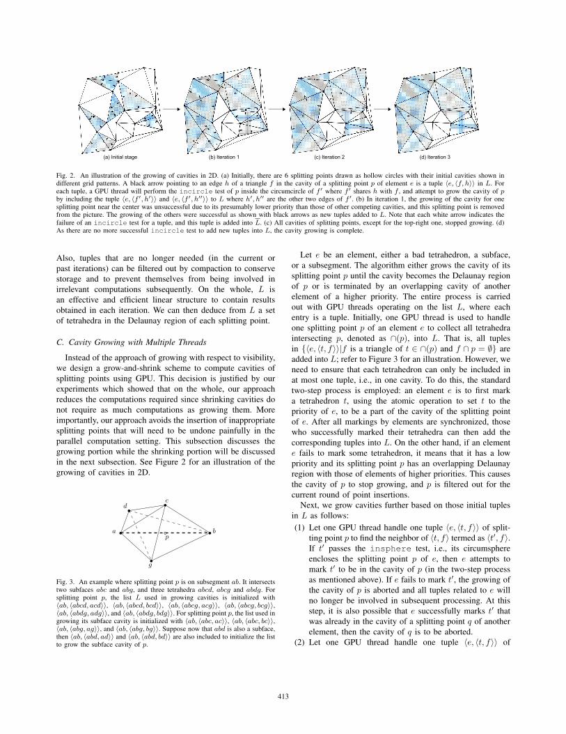
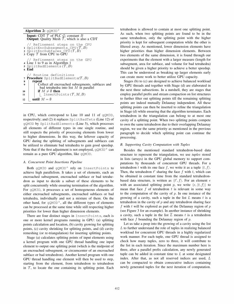
Fig. 2. An illustration of the growing of cavities in 2D. (a) Initially, there are 6 splitting points drawn as hollow circles with their initial cavities shown indifferent grid patterns. A black arrow pointing to an edge h of a triangle f in the cavity of a splitting point p of element e is a tuple 〈e, 〈f, h〉〉 in L. Foreach tuple, a GPU thread will perform the incircle test of p inside the circumcircle of f ′ where f ′ shares h with f , and attempt to grow the cavity of pby including the tuple 〈e, 〈f ′, h′〉〉 and 〈e, 〈f ′, h′′〉〉 to L where h′, h′′ are the other two edges of f ′. (b) In iteration 1, the growing of the cavity for onesplitting point near the center was unsuccessful due to its presumably lower priority than those of other competing cavities, and this splitting point is removedfrom the picture. The growing of the others were successful as shown with black arrows as new tuples added to L. Note that each white arrow indicates thefailure of an incircle test for a tuple, and this tuple is added into L. (c) All cavities of splitting points, except for the top-right one, stopped growing. (d)As there are no more successful incircle test to add new tuples into L, the cavity growing is complete.

Also, tuples that are no longer needed (in the current or

past iterations) can be filtered out by compaction to conserve

storage and to prevent themselves from being involved in

irrelevant computations subsequently. On the whole, L is

an effective and efficient linear structure to contain results

obtained in each iteration. We can then deduce from L a set

of tetrahedra in the Delaunay region of each splitting point.

C. Cavity Growing with Multiple Threads

Instead of the approach of growing with respect to visibility,

we design a grow-and-shrink scheme to compute cavities of

splitting points using GPU. This decision is justified by our

experiments which showed that on the whole, our approach

reduces the computations required since shrinking cavities do

not require as much computations as growing them. More

importantly, our approach avoids the insertion of inappropriate

splitting points that will need to be undone painfully in the

parallel computation setting. This subsection discusses the

growing portion while the shrinking portion will be discussed

in the next subsection. See Figure 2 for an illustration of the

growing of cavities in 2D.

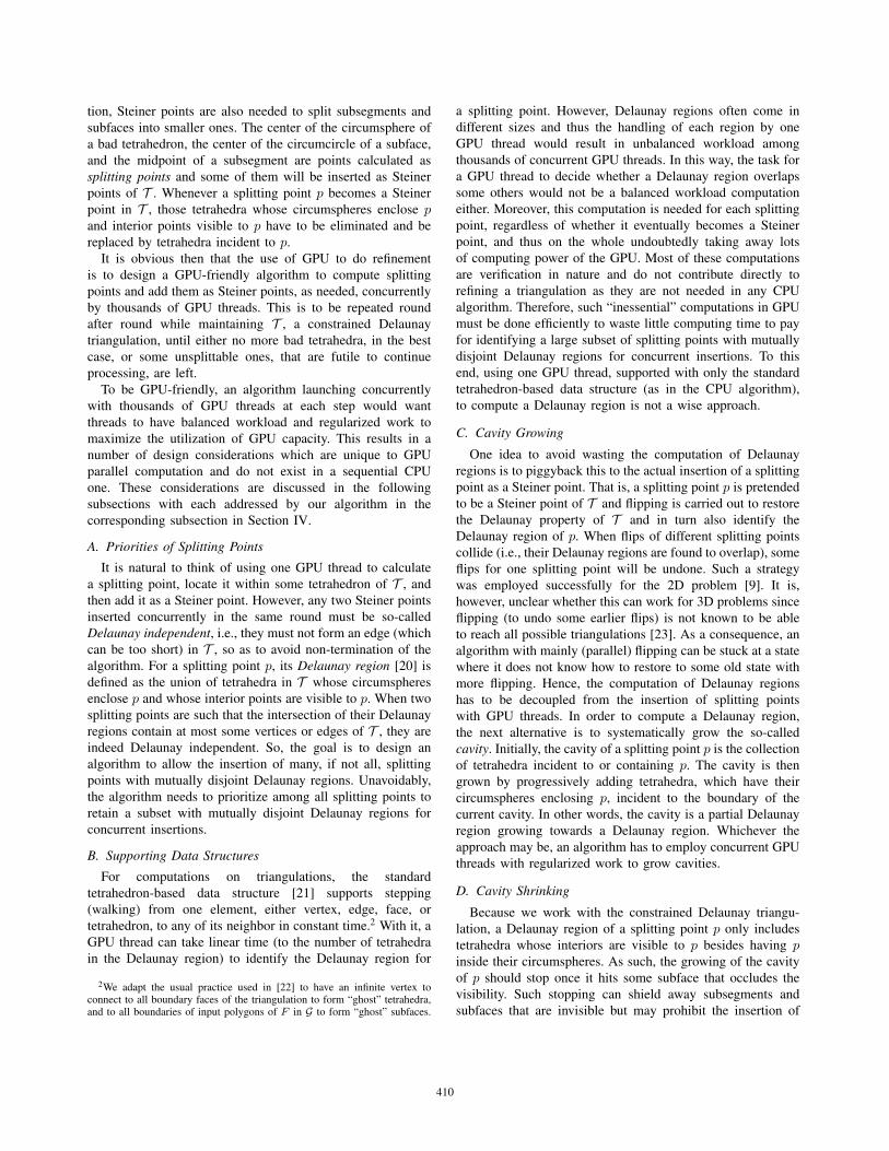
a bp

cd

g

Fig. 3. An example where splitting point p is on subsegment ab. It intersectstwo subfaces abc and abg, and three tetrahedra abcd, abcg and abdg. Forsplitting point p, the list L used in growing cavities is initialized with〈ab, 〈abcd, acd〉〉, 〈ab, 〈abcd, bcd〉〉, 〈ab, 〈abcg, acg〉〉, 〈ab, 〈abcg, bcg〉〉,〈ab, 〈abdg, adg〉〉, and 〈ab, 〈abdg, bdg〉〉. For splitting point p, the list used ingrowing its subface cavity is initialized with 〈ab, 〈abc, ac〉〉, 〈ab, 〈abc, bc〉〉,〈ab, 〈abg, ag〉〉, and 〈ab, 〈abg, bg〉〉. Suppose now that abd is also a subface,then 〈ab, 〈abd, ad〉〉 and 〈ab, 〈abd, bd〉〉 are also included to initialize the listto grow the subface cavity of p.

Let e be an element, either a bad tetrahedron, a subface,

or a subsegment. The algorithm either grows the cavity of its

splitting point p until the cavity becomes the Delaunay region

of p or is terminated by an overlapping cavity of another

element of a higher priority. The entire process is carried

out with GPU threads operating on the list L, where each

entry is a tuple. Initially, one GPU thread is used to handle

one splitting point p of an element e to collect all tetrahedra

intersecting p, denoted as ∩(p), into L. That is, all tuples

in {〈e, 〈t, f〉〉|f is a triangle of t ∈ ∩(p) and f ∩ p = ∅} are

added into L; refer to Figure 3 for an illustration. However, we

need to ensure that each tetrahedron can only be included in

at most one tuple, i.e., in one cavity. To do this, the standard

two-step process is employed: an element e is to first mark

a tetrahedron t, using the atomic operation to set t to the

priority of e, to be a part of the cavity of the splitting point

of e. After all markings by elements are synchronized, those

who successfully marked their tetrahedra can then add the

corresponding tuples into L. On the other hand, if an element

e fails to mark some tetrahedron, it means that it has a low

priority and its splitting point p has an overlapping Delaunay

region with those of elements of higher priorities. This causes

the cavity of p to stop growing, and p is filtered out for the

current round of point insertions.

Next, we grow cavities further based on those initial tuples

in L as follows:

(1) Let one GPU thread handle one tuple 〈e, 〈t, f〉〉 of split-

ting point p to find the neighbor of 〈t, f〉 termed as 〈t′, f〉.If t′ passes the insphere test, i.e., its circumsphere

encloses the splitting point p of e, then e attempts to

mark t′ to be in the cavity of p (in the two-step process

as mentioned above). If e fails to mark t′, the growing of

the cavity of p is aborted and all tuples related to e will

no longer be involved in subsequent processing. At this

step, it is also possible that e successfully marks t′ that

was already in the cavity of a splitting point q of another

element, then the cavity of q is to be aborted.

(2) Let one GPU thread handle one tuple 〈e, 〈t, f〉〉 of

413

splitting point p to find the neighbor of 〈t, f〉 termed

as 〈t′, f〉. If t′ passes the insphere test, then we add

all tuples in {〈e, 〈t′, f ′〉〉|f ′ �= f is a triangle of t′} to

L; otherwise, we add 〈e, 〈t′, f〉〉 to L, which is a list to

keep track of all tetrahedra which failed the inspheretest and are to be used subsequently in the shrinking of

cavities.

(3) If new tuples were added to L in Step 2, go to Step 1

and repeat the process for the new tuples; otherwise stop.

When the above terminates, each element with tuples that

always succeeded in marking tetrahedra during the process

has identified the (more than) complete Delaunay region of

its splitting point. Moreover, all such Delaunay regions of

splitting points are disjoint.

The above works for cavities that are formed by collections

of tetrahedra. As subfaces are constraints from the input that

we need to split into smaller ones in the output, we also need to

identify the so-called subface cavities. The process of growing

with triangles in a subface cavity here has the same structure as

that of growing with tetrahedra in a cavity with the following

adjustments: (1) the incircle test, which decides whether

a point is inside a circumcircle of a triangle, is used instead

of the insphere test; and (2) growing with triangles is to

respect the visibility and thus does not cross any subsegment,

while growing with tetrahedra can cross subfaces.

Though the above has identified splitting points with disjoint

Delaunay regions, not all splitting points can be inserted into Tas yet. We do not insert splitting points of bad tetrahedra that

encroach upon existing subfaces or subsegments, and do not

insert those of subfaces that encroach upon existing subseg-

ments. Such splitting points have to wait until later rounds after

those encroached subfaces and encroached subsegments have

been split. This is to respect the priority of splitting elements

of lower dimensions before those of higher dimensions. The

growing of a cavity without concerning occlusions due to

subfaces, in our algorithm, allows us to easily identify those

splitting points that are not good for insertion as follows: we

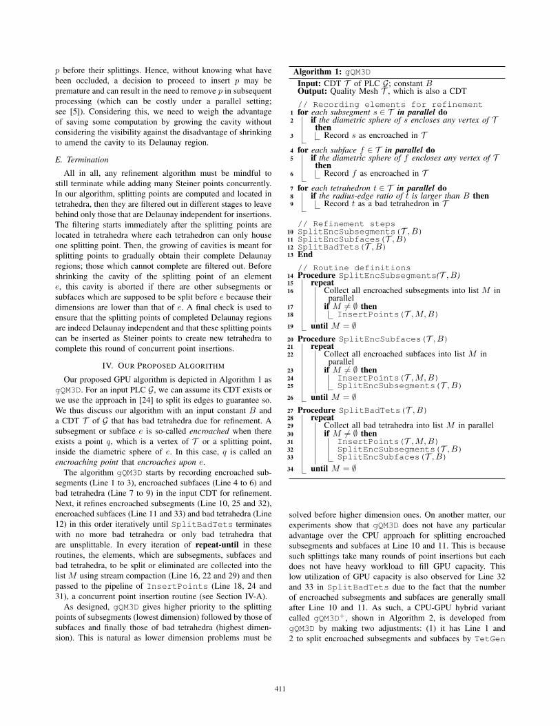
assign one GPU thread to handle one tuple, 〈e, 〈t, f〉〉, in Lwhere p is the splitting point of e. If e is a bad tetrahedron

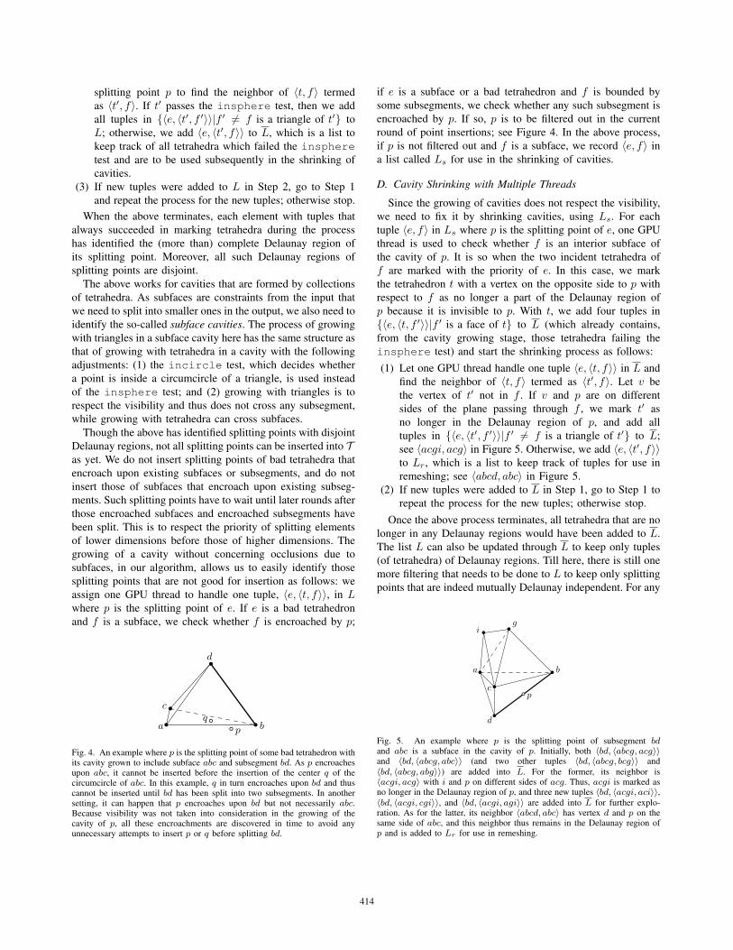
and f is a subface, we check whether f is encroached by p;

a b

c

d

p

q

Fig. 4. An example where p is the splitting point of some bad tetrahedron withits cavity grown to include subface abc and subsegment bd. As p encroachesupon abc, it cannot be inserted before the insertion of the center q of thecircumcircle of abc. In this example, q in turn encroaches upon bd and thuscannot be inserted until bd has been split into two subsegments. In anothersetting, it can happen that p encroaches upon bd but not necessarily abc.Because visibility was not taken into consideration in the growing of thecavity of p, all these encroachments are discovered in time to avoid anyunnecessary attempts to insert p or q before splitting bd.

if e is a subface or a bad tetrahedron and f is bounded by

some subsegments, we check whether any such subsegment is

encroached by p. If so, p is to be filtered out in the current

round of point insertions; see Figure 4. In the above process,

if p is not filtered out and f is a subface, we record 〈e, f〉 in

a list called Ls for use in the shrinking of cavities.

D. Cavity Shrinking with Multiple Threads

Since the growing of cavities does not respect the visibility,

we need to fix it by shrinking cavities, using Ls. For each

tuple 〈e, f〉 in Ls where p is the splitting point of e, one GPU

thread is used to check whether f is an interior subface of

the cavity of p. It is so when the two incident tetrahedra of

f are marked with the priority of e. In this case, we mark

the tetrahedron t with a vertex on the opposite side to p with

respect to f as no longer a part of the Delaunay region of

p because it is invisible to p. With t, we add four tuples in

{〈e, 〈t, f ′〉〉|f ′ is a face of t} to L (which already contains,

from the cavity growing stage, those tetrahedra failing the

insphere test) and start the shrinking process as follows:

(1) Let one GPU thread handle one tuple 〈e, 〈t, f〉〉 in L and

find the neighbor of 〈t, f〉 termed as 〈t′, f〉. Let v be

the vertex of t′ not in f . If v and p are on different

sides of the plane passing through f , we mark t′ as

no longer in the Delaunay region of p, and add all

tuples in {〈e, 〈t′, f ′〉〉|f ′ �= f is a triangle of t′} to L;

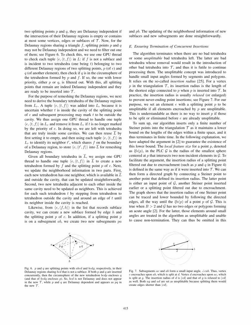
see 〈acgi, acg〉 in Figure 5. Otherwise, we add 〈e, 〈t′, f〉〉to Lr, which is a list to keep track of tuples for use in

remeshing; see 〈abcd, abc〉 in Figure 5.

(2) If new tuples were added to L in Step 1, go to Step 1 to

repeat the process for the new tuples; otherwise stop.

Once the above process terminates, all tetrahedra that are no

longer in any Delaunay regions would have been added to L.

The list L can also be updated through L to keep only tuples

(of tetrahedra) of Delaunay regions. Till here, there is still one

more filtering that needs to be done to L to keep only splitting

points that are indeed mutually Delaunay independent. For any

a b

c

d

ig

p

Fig. 5. An example where p is the splitting point of subsegment bdand abc is a subface in the cavity of p. Initially, both 〈bd, 〈abcg, acg〉〉and 〈bd, 〈abcg, abc〉〉 (and two other tuples 〈bd, 〈abcg, bcg〉〉 and

〈bd, 〈abcg, abg〉〉) are added into L. For the former, its neighbor is〈acgi, acg〉 with i and p on different sides of acg. Thus, acgi is marked asno longer in the Delaunay region of p, and three new tuples 〈bd, 〈acgi, aci〉〉,〈bd, 〈acgi, cgi〉〉, and 〈bd, 〈acgi, agi〉〉 are added into L for further explo-ration. As for the latter, its neighbor 〈abcd, abc〉 has vertex d and p on thesame side of abc, and this neighbor thus remains in the Delaunay region ofp and is added to Lr for use in remeshing.

414

two splitting points p and q, they are Delaunay independent if

the intersection of their Delaunay regions is empty or contains

at most some vertices, edges or subfaces of T . Now, for the

Delaunay regions sharing a triangle f , splitting points p and qmay not be Delaunay independent and we need to filter out one

of them; see Figure 6. To check this, we use one GPU thread

to check each tuple 〈e, 〈t, f〉〉 in L: if f is not a subface and

is incident to two tetrahedra (one being t) belonging to two

different Delaunay regions of two splitting points, p (of e) and

q (of another element), then check if q is in the circumsphere of

the tetrahedron formed by p and f . If so, the one with lower

priority, either p or q, is filtered out. With this, all splitting

points that remain are indeed Delaunay independent and they

are ready to be inserted into T .

For the purpose of remeshing the Delaunay regions, we next

need to derive the boundary tetrahedra of the Delaunay regions

from Lr. A tuple 〈e, 〈t, f〉〉 was added into Lr because it is

uncertain whether t is inside the cavity of the splitting point

of e and subsequent processing may mark t to be outside the

cavity. We thus assign one GPU thread to handle one tuple

〈e, 〈t, f〉〉 in Lr and remove it from Lr if t is no longer marked

by the priority of e. In doing so, we are left with tetrahedra

that are truly inside some cavities. We can then reuse L by

first setting it to empty, and then using each tuple 〈e, 〈t, f〉〉 in

Lr to identify its neighbor t′, which shares f on the boundary

of a Delaunay region, to store 〈e, 〈t′, f〉〉 into L for remeshing

Delaunay regions.

Given all boundary tetrahedra in L, we assign one GPU

thread to handle one tuple 〈e, 〈t, f〉〉 in L to create a new

tetrahedron formed by f and the splitting point p of e. Next,

we update the neighborhood information in two parts. First,

each new tetrahedron has one neighbor, which is available in Land outside the cavity, that can be updated straightforwardly.

Second, two new tetrahedra adjacent to each other inside the

same cavity need to be updated as neighbors. This is achieved

for each such tetrahedron t by stepping from tetrahedron to

tetrahedron outside the cavity and around an edge of t until

its neighbor inside the cavity is reached.

Likewise, from 〈e, 〈f, h〉〉 in the list that records subface

cavity, we can create a new subface formed by edge h and

the splitting point p of e. In addition, if a splitting point pis on a subsegment ab, we create two new subsegments pa

a

b

c

d gp q

Fig. 6. p and q are splitting points with abcd and bcdg, respectively, in theirDelaunay regions sharing bcd that is not a subface. If both p and q are insertedconcurrently, then the circumsphere of the new tetrahedron bcdp encloses q(and that of bcdq encloses p). So, bcd is not Delaunay and does not appearin the new T , while p and q are Delaunay dependent and appears as pq inthe new T .

and pb. The updating of the neighborhood information of new

subfaces and new subsegments are done straightforwardly.

E. Ensuring Termination of Concurrent Insertions

The algorithm terminates when there are no bad tetrahedra

or some unsplittable bad tetrahedra left. The latter are bad

tetrahedra whose removal would result in the introduction of

other bad tetrahedra into T , and thus it is futile to continue

processing them. The unsplittable concept was introduced to

handle small input angles formed by segments and polygons.

It relies on the so-called insertion radius [25]. For a vertex

p in the triangulation T , its insertion radius is the length of

the shortest edge connected to p when p is inserted into T . In

practice, the insertion radius is usually relaxed (or enlarged)

to prevent never-ending point insertions; see Figure 7. For our

purpose, we set an element e with a splitting point p to be

unsplittable if all elements encroached by p are unsplittable.

This is understandable as there is no way to insert p if those

to be split or eliminated before e are already unsplittable.

To sum up, our algorithm inserts only a finite number of

Steiner points into the triangulation T as it maintains a lower

bound on the lengths of the edges within a finite space, and it

thus terminates in finite time. In the following explanation, we

have adapted the argument in [2] to guarantee the existence of

this lower bound. The local feature size for a point p, denoted

as lfs(p), in the PLC G is the radius of the smallest sphere

centered at p that intersects two non-incident elements in G. To

facilitate the argument, the insertion radius of a splitting point

filtered out due to encroachment (such as p and q in Figure 4)

is defined in the same way as if it were inserted into T . We can

then form a directed graph by connecting a Steiner point to

another point that defined its insertion radius. The latter point

is either an input point of G, another Steiner point inserted

earlier or a splitting point filtered out due to encroachment.

The graph shows that the insertion radius of one Steiner point

can be traced and lower bounded by following the directed

edges, all the way until the lfs(p) of a point p of G. This is

true when B > 2 and G has no two edges or polygons forming

an acute angle [2]. For the latter, those elements around small

angles are treated in the algorithm as unsplittable and unable

to cause non-termination. They can thus be omitted in this

a b

c

d

g

Fig. 7. Subsegments ac and ab form a small input angle, � cab. Thus, vertexc encroaches upon ab, which is split at d. Vertex d encroaches upon ac, whichis split at g. The insertion radius of d is |cd| and that of g is relaxed to |cd|as well. Both ag and ad are set as unsplittable because splitting them wouldcreate edges shorter than |cd|.

415

discussion. Hence, the smallest lfs(p) bounds all the lengths

of edges in T .

V. EXPERIMENTAL RESULTS

All experiments were conducted on a PC with an Intel i7-

7700k 4.2GHz CPU, 32GB of DDR4 RAM and a GTX1080 Ti

graphics card with 11GB of video memory.

A. Software Used for Comparison

TetGen [3] is the main CPU software used as benchmark

for our work. Since CGAL [16] is a popular software in this

area, though its output often does not conform to its input PLC,

we incorporated it in our experiments with edge size = 5.0,

facet distance = 1.0 and cell radius edge ratio = B. As for

TetWild [17] that mainly focuses on robustness, it runs

rather slowly and is thus excluded from our study.

We implemented gQM3D and gQM3D+ using the CUDA

programming model of NVIDIA [26]. All computations in

GPU are done with the double precision. The exact arithmetic

and robust geometric predicates of Shewchuk [27] are adapted

from CPU to work in GPU. Simulation of Simplicity by

Edelsbrunner and Mucke [28] is used to deal with degenerate

cases.

In our implementation, we chose to stop the growing of

a cavity when it ran beyond a large number of iterations,

such as in the case of a degenerate tetrahedron. We set such a

tetrahedron to unsplittable when encountered. This, however,

did not result in any significant increase in the number of bad

tetrahedra in the outputs of our experiments. In another aspect,

we noticed that a cavity of p that caused another of say q to

stop growing, may itself be forbidden to be grown by other

cavities. The question is then whether it is worthwhile to revive

the growing of the cavity of q since its needed tetrahedra are

now made available through p. With regards to this, we have

attempted some approaches in our implementation but have

yet to find any good one which improves performance.

All software were compiled with all optimization flags

turned on. The input to all software is a PLC with a constant

B. We used TetGen to generate the initial CDT (that has

bad tetrahedra) to be refined by gQM3D and gQM3D+. In

measuring computing time, we included the time of computing

the CDT of the input PLC in all software. We have done

experiments on both synthetic and real-world datasets as

reported in the following two subsections.

B. Synthetic Dataset

To better understand the behavior of the various software

and to stress test them, we generated PLCs with points in the

following distributions: uniform, Gaussian, ball (where points

lie randomly in a ball) and sphere (where points lie randomly

within the thin shell formed by two concentric spheres with

different radii). Also, we randomly generated polygons that

are rectangles to add into our PLCs. While edges of rectangles

may form small input angles among themselves, we ensured

that there were no intersections among them, except at their

endpoints.

The number of input points in each PLC is between 10K to

30K, while the ratio of the number of rectangles to the number

of points, denoted as γ, ranges from 0.05 to 0.25. These

parameters were chosen to stress test gQM3D and gQM3D+

by exhausting the available GPU memory, which supports

output sizes of over tens of millions of points and tetrahedra.

Although the termination of the various software requires

B > 2 and input angles no less than 90◦, this is less onerous in

practice. We thus tried a spread of B, around 2, and let gQM3Dand gQM3D+ adapt the same approach as TetGen to handle

elements in the vicinity of small input angles. Consequently,

the output triangulations can contain some bad tetrahedra that

are unsplittable due to small input angles.

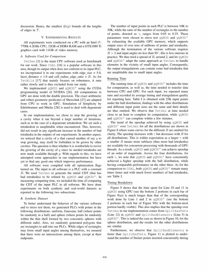
Running Time

The running time of gQM3D and gQM3D+ includes the time

for computation, as well as, the time needed to transfer data

between CPU and GPU. For each input, we repeated many

runs and recorded its average timing and triangulation quality

for reporting here. Table I is obtained with 25K input points

under the ball distribution; findings with the other distributions

and different input point sizes are the same and their details

are thus omitted. We observe that TetGen at time needed

close to an hour to complete its computation, while gQM3Dand gQM3D+ can complete within a few minutes.

The trend of the speedup achieved by using gQM3D and

gQM3D+ over TetGen for all the distributions are shown in

Figure 8 where some curves for the different B are omitted for

clarity. The speedup increases with γ but decreases with B for

all distributions. This is within expectation as a larger γ with

a smaller B means more subfaces (thus more bad tetrahedra)

are available for concurrent processing with thousands of GPU

threads. As a result, gQM3D and gQM3D+ can achieve speedup

of an order of magnitude. Across the four distributions, for

each γ, we note that gQM3D and gQM3D+ have consistently

achieved a higher speedup with the ball distribution, while

having comparable performance on the other three. As for the

comparison to CGAL, both gQM3D and gQM3D+ remain many

times faster and with much fewer numbers of bad tetrahedra;

see Table I.

Timing Breakdown

Figure 9 shows that the time spent for Line 10 and 11 in

gQM3D using GPU (see the bottom 2 portions in each bar of

Figure 9(a)) is much longer than that of the corresponding

work done by Line 1 and 2 in gQM3D+ (see the bottom

2 portions in each bar of Figure 9(b) with the bottom-most

portion hardly visible). This also implies that the speedup over

TetGen in our implementation comes from SplitBadTets(Line 12) in gQM3D and SplitBadElements (Line 5) in

gQM3D+. This is indeed the case as shown in Figure 10, for the

sphere distribution, and the results for the other distributions

are similar.

Furthermore, we observe that SplitBadElements is

faster than SplitBadTets. Figure 11 is plotted to under-

stand the number of Steiner points inserted concurrently during

416

γ 0.05 0.10 0.15 0.20 0.25

SoftwareCGAL TetGen gQM3D gQM3D+ CGAL TetGen gQM3D gQM3D+ CGAL TetGen gQM3D gQM3D+ CGAL TetGen gQM3D gQM3D+ CGAL TetGen gQM3D gQM3D+

B1.4Time (min) 2.8 2.5 1.3 0.5 6.9 6.6 2.2 0.9 11.1 20.4 3.1 1.7 15.7 28.6 3.9 1.9 21.3 53.4 4.5 2.5

Points (M) 0.78 0.95 0.93 0.96 1.46 1.52 1.49 1.54 2.09 2.63 2.59 2.67 2.62 3.11 3.06 3.16 3.24 4.24 4.18 4.29

Tets (M) 4.99 5.98 5.85 6.07 9.29 9.58 9.40 9.74 13.29 16.68 16.37 16.89 16.65 19.67 19.35 20.01 20.57 26.89 26.44 27.24

Bad Tets > 1M 401 308 391 > 2M 1461 1416 1485 > 2M 2160 2059 2230 > 3M 2885 2939 2871 > 4M 3677 3395 3680

1.6Time (min) 2.7 1.6 1.1 0.4 6.5 4.1 1.9 0.8 10.5 12.8 3.4 1.4 15.0 18.3 3.4 1.7 20.8 34.3 4.1 2.3

Points (M) 0.66 0.68 0.69 0.69 1.22 1.12 1.13 1.13 1.74 2.03 2.06 2.05 2.19 2.39 2.44 2.42 2.70 3.33 3.39 3.37

Tets (M) 4.19 4.27 4.33 4.33 7.76 7.00 7.10 7.09 11.10 12.73 12.91 12.90 13.91 15.06 15.29 15.26 17.17 20.94 21.28 21.24

Bad Tets > 0.8M 303 252 313 > 1M 1279 1152 1212 > 2M 1877 1725 1870 > 2M 2520 2355 2472 > 3M 3235 2924 3261

1.8Time (min) 2.6 1.1 1.1 0.4 6.3 2.9 1.7 0.7 10.2 9.0 2.5 1.3 14.2 12.8 3.3 1.6 19.3 24.1 4.6 2.0

Points (M) 0.59 0.56 0.57 0.57 1.09 0.92 0.95 0.94 1.55 1.73 1.79 1.75 1.95 2.05 2.12 2.07 2.40 2.88 2.97 2.93

Tets (M) 3.76 3.46 3.57 3.53 6.90 5.74 5.93 5.83 9.87 10.76 11.10 10.92 12.38 12.75 13.16 12.92 15.29 17.94 18.51 18.27

Bad Tets > 0.7M 251 229 250 > 1M 1083 1467 1122 > 1M 1599 1473 1585 > 2M 1998 2004 1978 > 2M 2696 2484 2708

2.0Time (min) 2.4 0.8 1.0 0.3 5.9 2.2 1.8 0.6 9.4 6.9 2.6 1.2 13.3 9.7 3.1 1.5 18.3 18.5 3.6 1.9

Points (M) 0.55 0.49 0.51 0.50 1.00 0.82 0.85 0.83 1.43 1.57 1.62 1.60 1.80 1.86 1.92 1.88 2.22 2.63 2.73 2.67

Tets (M) 3.50 3.02 3.14 3.10 6.39 5.06 5.26 5.16 9.14 9.66 10.03 9.87 11.46 11.48 11.89 11.61 14.14 16.25 16.85 16.51

Bad Tets > 0.6M 232 201 226 > 1.2M 967 935 1004 > 1.6M 1381 1294 1375 > 2.0M 1746 1670 1751 > 2.6M 2330 2149 2380

TABLE IEXPERIMENTAL RESULTS WITH 25K INPUT POINTS OF THE BALL DISTRIBUTION. “TETS” DENOTES TETRAHEDRA.

0.05 0.1 0.15 0.2 0.250

4

8

12

16

20

24

Spe

edup

(a) Uniform

0.05 0.1 0.15 0.2 0.250

4

8

12

16

20

24

Spe

edup

(b) Gaussian

0.05 0.1 0.15 0.2 0.250

4

8

12

16

20

24

Spe

edup

(c) Ball

0.05 0.1 0.15 0.2 0.250

4

8

12

16

20

24

Spe

edup

(d) Sphere

Fig. 8. Speedup of gQM3D and gQM3D+ in the various distributions.

Fig. 9. Timing breakdown of gQM3D and gQM3D+ in different distributionswith B = 1.4 and γ = 0.25.

the process. We see that SplitBadTets gradually increases

the performance of inserting more Steiner points but being

interrupted regularly along the way, with low performance of

inserting fewer Steiner points (due to Line 32 and 33). The per-

formance then decreases towards the end of the computation

with a long tail. On the other hand, SplitBadElementsquickly jumps to high performance and consistently maintains

high performance until it decays quickly to end the computa-

tion. This demonstrates that gQM3D+ is able to maintain high

utilization of GPU capacity to complete its computation as it

0.05 0.1 0.15 0.2 0.250

5

10

15

20

25

30

Spe

edup

Fig. 10. The speedup of SplitBadTets and of SplitBadElementswhen compared to the corresponding routine in TetGen for the spheredistribution.

Fig. 11. General pattern of concurrency in (a) SplitBadTets and (b)SplitBadElements. This is on a sphere distribution with 20K input points,γ = 0.25, B = 1.4, and 4M output points.

has parallelism within the splitting of each type of elements,

as well as, parallelism across different types of elements.

Output Sizes

Table I also shows the number of points in the output

417

1.4 1.6 1.8 2

B

-3

-2

-1

0

1

2

3

4P

erce

ntag

eUniform Gaussian Ball Sphere

1.4 1.6 1.8 2

B

-3

-2

-1

0

1

2

3

4

Per

cent

age

Fig. 12. Comparison (in percentage difference) of the number of Steinerpoints in the output triangulations of gQM3D, gQM3D+ and TetGen forγ = 0.05. Negative means fewer Steiner points in our software while positivemeans otherwise.

Fig. 13. The distributions of dihedral angles in the output triangulations ofSculpture as generated by the various software.

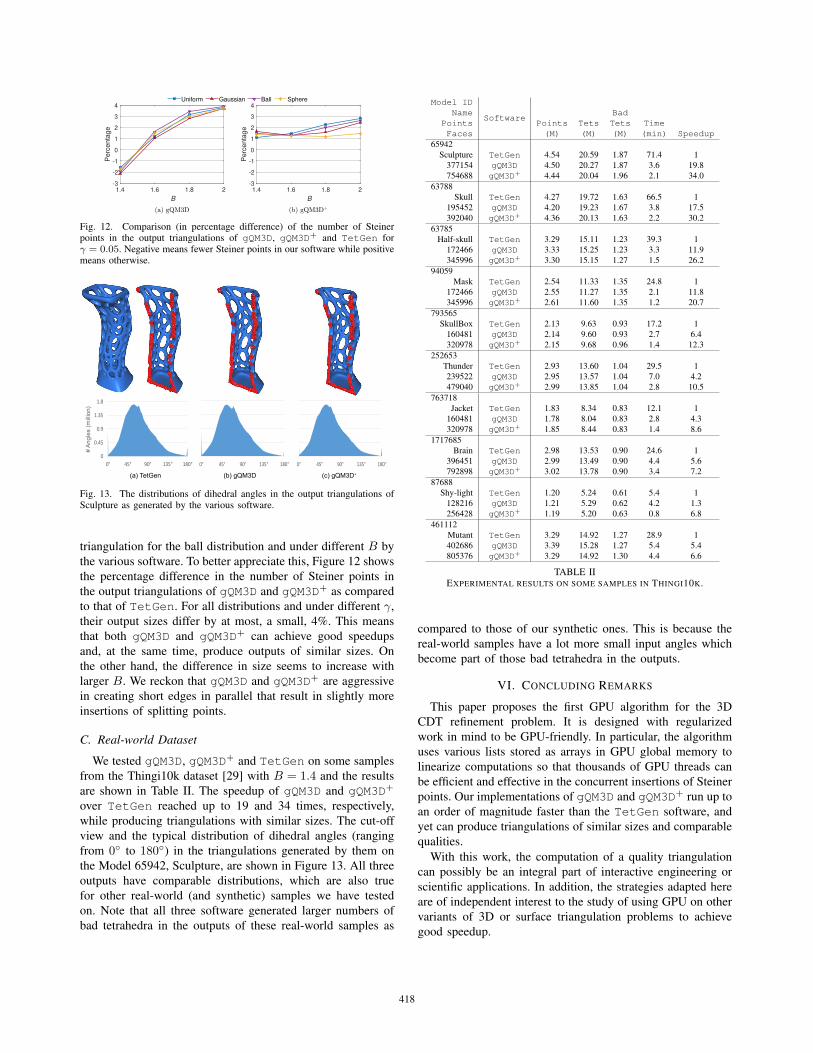
triangulation for the ball distribution and under different B by

the various software. To better appreciate this, Figure 12 shows

the percentage difference in the number of Steiner points in

the output triangulations of gQM3D and gQM3D+ as compared

to that of TetGen. For all distributions and under different γ,

their output sizes differ by at most, a small, 4%. This means

that both gQM3D and gQM3D+ can achieve good speedups

and, at the same time, produce outputs of similar sizes. On

the other hand, the difference in size seems to increase with

larger B. We reckon that gQM3D and gQM3D+ are aggressive

in creating short edges in parallel that result in slightly more

insertions of splitting points.

C. Real-world Dataset

We tested gQM3D, gQM3D+ and TetGen on some samples

from the Thingi10k dataset [29] with B = 1.4 and the results

are shown in Table II. The speedup of gQM3D and gQM3D+

over TetGen reached up to 19 and 34 times, respectively,

while producing triangulations with similar sizes. The cut-off

view and the typical distribution of dihedral angles (ranging

from 0◦ to 180◦) in the triangulations generated by them on

the Model 65942, Sculpture, are shown in Figure 13. All three

outputs have comparable distributions, which are also true

for other real-world (and synthetic) samples we have tested

on. Note that all three software generated larger numbers of

bad tetrahedra in the outputs of these real-world samples as

Model ID

SoftwareName Bad

Points Points Tets Tets TimeFaces (M) (M) (M) (min) Speedup

65942

Sculpture TetGen 4.54 20.59 1.87 71.4 1

377154 gQM3D 4.50 20.27 1.87 3.6 19.8

754688 gQM3D+ 4.44 20.04 1.96 2.1 34.0

63788

Skull TetGen 4.27 19.72 1.63 66.5 1

195452 gQM3D 4.20 19.23 1.67 3.8 17.5

392040 gQM3D+ 4.36 20.13 1.63 2.2 30.2

63785

Half-skull TetGen 3.29 15.11 1.23 39.3 1

172466 gQM3D 3.33 15.25 1.23 3.3 11.9

345996 gQM3D+ 3.30 15.15 1.27 1.5 26.2

94059

Mask TetGen 2.54 11.33 1.35 24.8 1

172466 gQM3D 2.55 11.27 1.35 2.1 11.8

345996 gQM3D+ 2.61 11.60 1.35 1.2 20.7

793565

SkullBox TetGen 2.13 9.63 0.93 17.2 1

160481 gQM3D 2.14 9.60 0.93 2.7 6.4

320978 gQM3D+ 2.15 9.68 0.96 1.4 12.3

252653

Thunder TetGen 2.93 13.60 1.04 29.5 1

239522 gQM3D 2.95 13.57 1.04 7.0 4.2

479040 gQM3D+ 2.99 13.85 1.04 2.8 10.5

763718

Jacket TetGen 1.83 8.34 0.83 12.1 1

160481 gQM3D 1.78 8.04 0.83 2.8 4.3

320978 gQM3D+ 1.85 8.44 0.83 1.4 8.6

1717685

Brain TetGen 2.98 13.53 0.90 24.6 1

396451 gQM3D 2.99 13.49 0.90 4.4 5.6

792898 gQM3D+ 3.02 13.78 0.90 3.4 7.2

87688

Shy-light TetGen 1.20 5.24 0.61 5.4 1

128216 gQM3D 1.21 5.29 0.62 4.2 1.3

256428 gQM3D+ 1.19 5.20 0.63 0.8 6.8

461112

Mutant TetGen 3.29 14.92 1.27 28.9 1

402686 gQM3D 3.39 15.28 1.27 5.4 5.4

805376 gQM3D+ 3.29 14.92 1.30 4.4 6.6

TABLE IIEXPERIMENTAL RESULTS ON SOME SAMPLES IN THINGI10K.

compared to those of our synthetic ones. This is because the

real-world samples have a lot more small input angles which

become part of those bad tetrahedra in the outputs.

VI. CONCLUDING REMARKS

This paper proposes the first GPU algorithm for the 3D

CDT refinement problem. It is designed with regularized

work in mind to be GPU-friendly. In particular, the algorithm

uses various lists stored as arrays in GPU global memory to

linearize computations so that thousands of GPU threads can

be efficient and effective in the concurrent insertions of Steiner

points. Our implementations of gQM3D and gQM3D+ run up to

an order of magnitude faster than the TetGen software, and

yet can produce triangulations of similar sizes and comparable

qualities.

With this work, the computation of a quality triangulation

can possibly be an integral part of interactive engineering or

scientific applications. In addition, the strategies adapted here

are of independent interest to the study of using GPU on other

variants of 3D or surface triangulation problems to achieve

good speedup.

418

REFERENCES

[1] G. L. Miller, “Control Volume Meshes Using Sphere Packing,” in Solv-ing Irregularly Structured Problems in Parallel, A. Ferreira, J. Rolim,H. Simon, and S.-H. Teng, Eds. Berlin, Heidelberg: Springer BerlinHeidelberg, 1998, pp. 128–131.

[2] J. R. Shewchuk, “Tetrahedral Mesh Generation by Delaunay Refine-ment,” in Proceedings of the Fourteenth Annual Symposium on Compu-tational Geometry. New York, NY, USA: ACM, 1998, pp. 86–95.

[3] H. Si, “TetGen, a Delaunay-Based Quality Tetrahedral Mesh Generator,”ACM Trans. Math. Softw., vol. 41, no. 2, pp. 11:1–11:36, Feb. 2015.

[4] C. Marot, J. Pellerin, and J. Remacle, “One Machine, One Minute,Three Billion Tetrahedra,” CoRR, vol. abs/1805.08831, 2018. [Online].Available: http://arxiv.org/abs/1805.08831

[5] P. Foteinos and N. Chrisochoides, “Dynamic Parallel 3D DelaunayTriangulation,” in Proceedings of the 20th International MeshingRoundtable, W. R. Quadros, Ed. Berlin, Heidelberg: Springer BerlinHeidelberg, 2012, pp. 3–20.

[6] L. P. Chew, “Guaranteed-Quality Triangular Meshes,” Department ofComputer Science, Cornell University, Tech. Rep. 89–983, 1989.

[7] ——, “Guaranteed-Quality Mesh Generation for Curved Surfaces,” inProceedings of the Ninth Annual Symposium on Computational Geom-etry. ACM, 1993, pp. 274–280.

[8] J. Ruppert, “A Delaunay Refinement Algorithm for Quality 2-Dimensional Mesh Generation,” J. Algorithms, vol. 18, no. 3, pp. 548–585, May 1995.

[9] Z. Chen, M. Qi, and T.-S. Tan, “Computing Delaunay Refinement Usingthe GPU,” in Proceedings of the 21st ACM SIGGRAPH Symposium onInteractive 3D Graphics and Games. New York, NY, USA: ACM,2017, pp. 11:1–11:9.

[10] T. K. Dey, C. L. Bajaj, and K. Sugihara, “On Good Triangulations inThree Dimensions,” in Proceedings of the First ACM Symposium onSolid Modeling Foundations and CAD/CAM Applications. New York,NY, USA: ACM, 1991, pp. 431–441.

[11] L. P. Chew, “Guaranteed-Quality Delaunay Meshing in 3D (ShortVersion),” in Proceedings of the Thirteenth Annual Symposium onComputational Geometry. New York, NY, USA: ACM, 1997, pp. 391–393.

[12] J. R. Shewchuk, “Constrained Delaunay Tetrahedralizations and Prov-ably Good Boundary Recovery,” in Eleventh International MeshingRoundtable, 2002, pp. 193–204.

[13] H. Si, “Constrained Delaunay Tetrahedral Mesh Generation and Refine-ment,” Finite Elements in Analysis and Design, vol. 46, no. 1-2, pp.33–46, 2010.

[14] S. Oudot, L. Rineau, and M. Yvinec, “Meshing Volumes Bounded bySmooth Surfaces,” in Proceedings of the 14th International MeshingRoundtable, B. W. Hanks, Ed. Berlin, Heidelberg: Springer BerlinHeidelberg, 2005, pp. 203–219.

[15] S.-W. Cheng, T. K. Dey, and J. A. Levine, “A Practical DelaunayMeshing Algorithm for a Large Class of Domains,” in Proceedings of the16th International Meshing Roundtable, M. L. Brewer and D. Marcum,Eds. Berlin, Heidelberg: Springer Berlin Heidelberg, 2008, pp. 477–494.

[16] P. Alliez, C. Jamin, L. Rineau, S. Tayeb, J. Tournois, andM. Yvinec, “3D Mesh Generation,” in CGAL User and ReferenceManual, 4.13 ed. CGAL Editorial Board, 2018. [Online]. Available:https://doc.cgal.org/4.13/Manual/packages.html#PkgMesh 3Summary

[17] Y. Hu, Q. Zhou, X. Gao, A. Jacobson, D. Zorin, and D. Panozzo,“Tetrahedral Meshing in the Wild,” ACM Trans. Graph., vol. 37, no. 4,pp. 60:1–60:14, Jul. 2018.

[18] D. K. Blandford, G. E. Blelloch, and C. Kadow, “Engineering a CompactParallel Delaunay Algorithm in 3D,” in Proceedings of the Twenty-second Annual Symposium on Computational Geometry. New York,NY, USA: ACM, 2006, pp. 292–300.

[19] A. N. Chernikov and N. P. Chrisochoides, “Three-Dimensional DelaunayRefinement for Multi-core Processors,” in Proceedings of the 22ndAnnual International Conference on Supercomputing. New York, NY,USA: ACM, 2008, pp. 214–224.

[20] P.-L. George and H. Borouchakin, Delaunay Triangulation and Meshing:Application to Finite Elements. Hermes Science Publications, 1998.

[21] L. Guibas and J. Stolfi, “Primitives for the Manipulation of GeneralSubdivisions and the Computation of Voronoi Diagrams,” ACM Trans.Graph., vol. 4, no. 2, pp. 74–123, Apr. 1985.

[22] J. R. Shewchuk, “Triangle: Engineering a 2D Quality Mesh Generatorand Delaunay Triangulator,” in Applied Computational Geometry To-wards Geometric Engineering, M. C. Lin and D. Manocha, Eds. Berlin,Heidelberg: Springer Berlin Heidelberg, 1996, pp. 203–222.

[23] B. Joe, “Three-Dimensional Triangulations from Local Transforma-tions,” SIAM J. Sci. and Stat. Comput., vol. 10, no. 4, pp. 718–741,1989.

[24] J. R. Shewchuk, “A Condition Guaranteeing the Existence of Higher-Dimensional Constrained Delaunay Triangulations,” in Proceedings ofthe Fourteenth Annual Symposium on Computational Geometry, 1998,pp. 76–85.

[25] J. R. Shewchuk and H. Si, “Higher-Quality Tetrahedral Mesh Generationfor Domains with Small Angles by Constrained Delaunay Refinement,”in Proceedings of the Thirtieth Annual Symposium on ComputationalGeometry. New York, NY, USA: ACM, 2014, pp. 290–299.

[26] J. Nickolls, I. Buck, M. Garland, and K. Skadron, “Scalable ParallelProgramming with CUDA,” Queue, vol. 6, no. 2, pp. 40–53, Mar. 2008.

[27] J. R. Shewchuk, “Adaptive Precision Floating-Point Arithmetic and FastRobust Geometric Predicates,” Discrete & Computational Geometry,vol. 18, pp. 305–368, 1997.

[28] H. Edelsbrunner and E. P. Mucke, “Simulation of Simplicity: A Tech-nique to Cope with Degenerate Cases in Geometric Algorithms,” ACMTrans. Graph., vol. 9, no. 1, pp. 66–104, Jan. 1990.

[29] Q. Zhou and A. Jacobson, “Thingi10K: A Dataset of 10,0003D-Printing Models,” CoRR, vol. abs/1605.04797, 2016. [Online].Available: http://arxiv.org/abs/1605.04797

419