


Languages
Pages
Legal


PHAS 3440 - 1 - Sherman Ip
Compton Scattering of Gamma Rays
Sherman Ip
Department of Physics and Astronomy, University College London [email protected]
Date submitted 12th November 2012
Using the gamma rays emitted from Caesium-137, gamma rays were scattered by colliding the gamma rays or photons with electrons in the scattering rod. As a result some of the photon energy was transferred to electrons and this transfer of energy is known as the Compton Effect. The experiment aims were to collect evidence of the Compton Effect and hence an experimental value of the electron mass was obtained.
PHAS 3440 - 2 - Sherman Ip
I. INTRODUCTION
Einstein postulated that light is 'quantized' as photons which can behave like particles or a
wave.4 A photon has energy which corresponds to the Plank’s energy, Eq. (1), and momentum
which corresponds to the de Broglie’s relationship, Eq. (2).4
(1) (energy of photon E, reduced Planck’s constant , angular frequency ω)
(2) (momentum p, wave vector k)
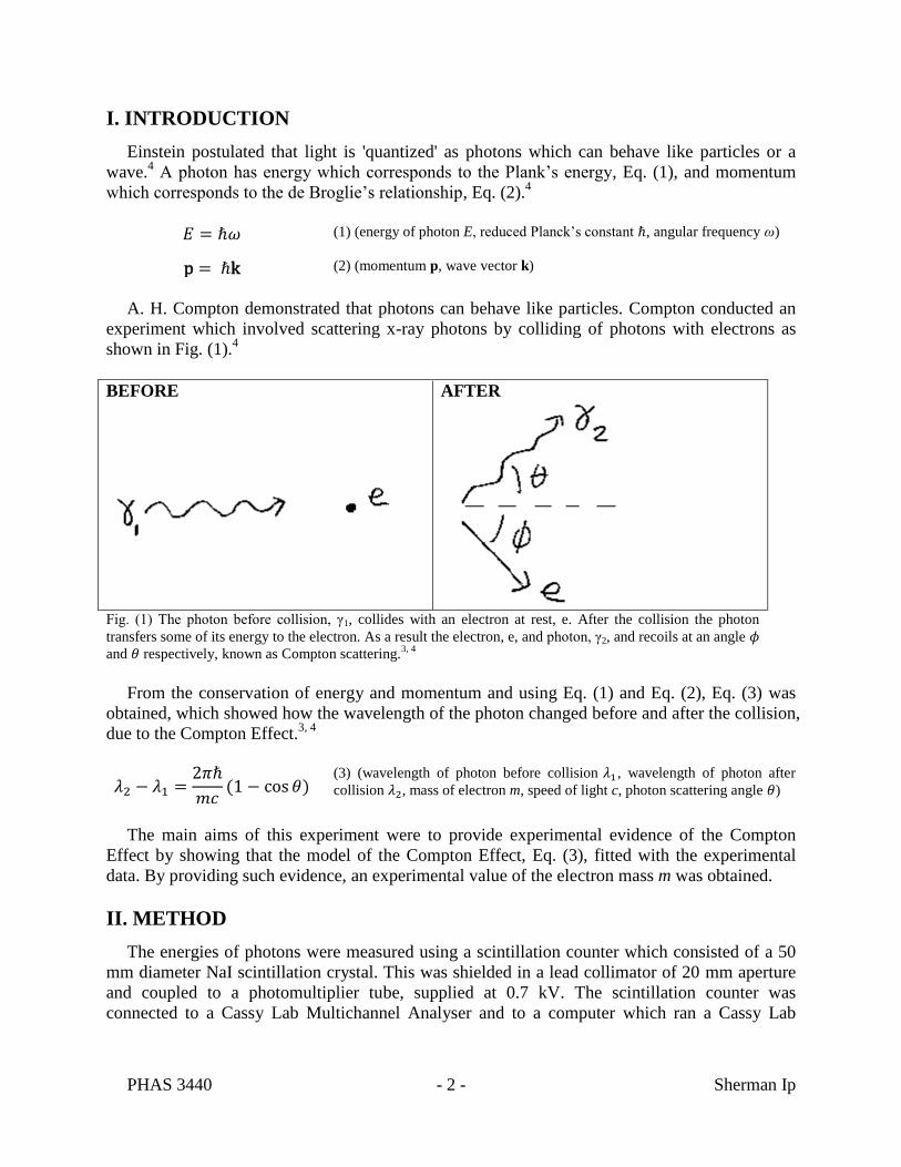
A. H. Compton demonstrated that photons can behave like particles. Compton conducted an
experiment which involved scattering x-ray photons by colliding of photons with electrons as
shown in Fig. (1).4
BEFORE
AFTER
Fig. (1) The photon before collision, γ1, collides with an electron at rest, e. After the collision the photon
transfers some of its energy to the electron. As a result the electron, e, and photon, γ2, and recoils at an angle
and respectively, known as Compton scattering.3, 4
From the conservation of energy and momentum and using Eq. (1) and Eq. (2), Eq. (3) was
obtained, which showed how the wavelength of the photon changed before and after the collision,
due to the Compton Effect.3, 4
(3) (wavelength of photon before collision , wavelength of photon after
collision , mass of electron m, speed of light c, photon scattering angle )
The main aims of this experiment were to provide experimental evidence of the Compton
Effect by showing that the model of the Compton Effect, Eq. (3), fitted with the experimental
data. By providing such evidence, an experimental value of the electron mass m was obtained.
II. METHOD
The energies of photons were measured using a scintillation counter which consisted of a 50
mm diameter NaI scintillation crystal. This was shielded in a lead collimator of 20 mm aperture
and coupled to a photomultiplier tube, supplied at 0.7 kV. The scintillation counter was
connected to a Cassy Lab Multichannel Analyser and to a computer which ran a Cassy Lab
PHAS 3440 - 3 - Sherman Ip
program. Cassy Lab recorded the energies of each photon, detected in the scintillation counter,
with a resolution of 1024 possible values of energy, ie 10 bits.
Caesium-137 (Cs-137) emits gamma rays of about 662 keV. 3
A Cs-137 source, with activity
of about , was placed in a lead block with a diameter hole. This
hopefully has produced a collimated beam of gamma rays, which was aimed directly at a
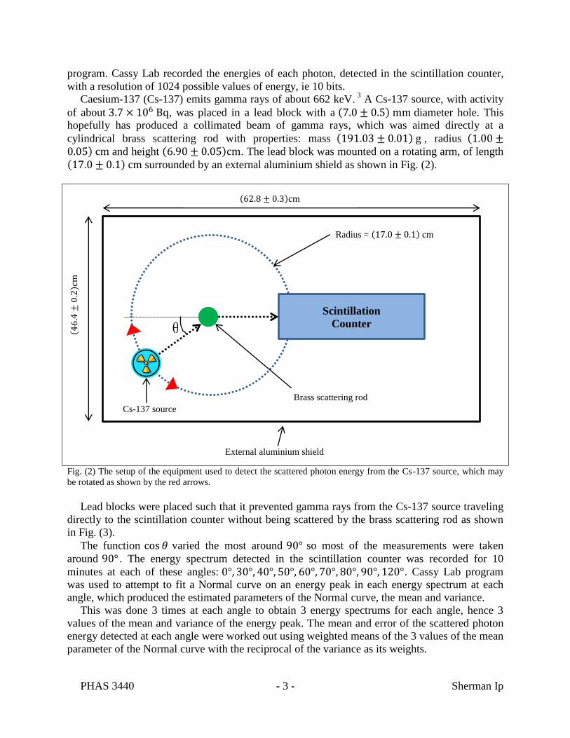
cylindrical brass scattering rod with properties: mass , radius and height . The lead block was mounted on a rotating arm, of length
surrounded by an external aluminium shield as shown in Fig. (2).
Fig. (2) The setup of the equipment used to detect the scattered photon energy from the Cs-137 source, which may
be rotated as shown by the red arrows.
Lead blocks were placed such that it prevented gamma rays from the Cs-137 source traveling
directly to the scintillation counter without being scattered by the brass scattering rod as shown
in Fig. (3).
The function varied the most around so most of the measurements were taken
around . The energy spectrum detected in the scintillation counter was recorded for 10
minutes at each of these angles: . Cassy Lab program
was used to attempt to fit a Normal curve on an energy peak in each energy spectrum at each
angle, which produced the estimated parameters of the Normal curve, the mean and variance.
This was done 3 times at each angle to obtain 3 energy spectrums for each angle, hence 3
values of the mean and variance of the energy peak. The mean and error of the scattered photon
energy detected at each angle were worked out using weighted means of the 3 values of the mean
parameter of the Normal curve with the reciprocal of the variance as its weights.
Brass scattering rod
Scintillation
Counter
Radius =
Cs-137 source
External aluminium shield

PHAS 3440 - 4 - Sherman Ip
Fig. (3) Lead blocks were placed between the Cs-137 and the scintillation counter to prevent gamma rays from the
Cs-137 travelling directly into the scintillation counter without being scattered.
An equation of the energy of photons before and after scattering was needed to model the
Compton Effect. Eq. (1) was substituted into Eq. (3) to obtain an equation for the change in the
energy of the photon due to the Compton Scattering as shown in Eq. (4).
[
]
(4) (energy of photon before collision , energy of
photon after collision )
For Cs-137, and which implied a model for the Compton Effect for Cs-137
was given in Eq. (5). 3
[
]
(5)
Eq. (4) was rearranged to form a linear regression as shown in Eq. (6), with intercept Eq. (7)
and gradient Eq. (8).
⏟
(
)
⏟
⏟
⏟
(6) (dependent variable y, independent variable x,
intercept a, gradient b)
(7)
(8)
PHAS 3440 - 5 - Sherman Ip
Therefore the expected gradient and intercept was worked out as shown in Eq. (9) and Eq.
(10) to 5 significant figures.
(9) (population or expected intercept , population or
accepted electron mass )
( to 3 significant figures)3
(10) (population or expected gradient )
Eq. (8) was subtracted from Eq. (7) which obtained an equation Eq. (11) which yielded a
value for the experimental electron mass, which used both the gradient and intercept with a given
error Eq. (12). Even though the value of was given of a value of , the standard
deviation must be estimated to consider all possible sources of error. 3
The mean and standard
deviation of were estimated using the mean and error respectively on measured at 0
degree.
(
⁄ )
(11)
(
⁄ ) √
(12) (error on the variable x )
III. RESULTS
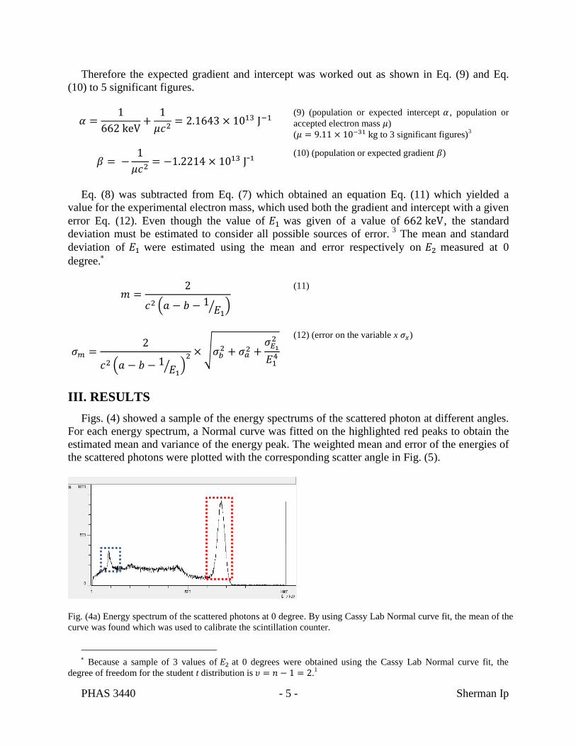
Figs. (4) showed a sample of the energy spectrums of the scattered photon at different angles.
For each energy spectrum, a Normal curve was fitted on the highlighted red peaks to obtain the
estimated mean and variance of the energy peak. The weighted mean and error of the energies of
the scattered photons were plotted with the corresponding scatter angle in Fig. (5).
Fig. (4a) Energy spectrum of the scattered photons at 0 degree. By using Cassy Lab Normal curve fit, the mean of the
curve was found which was used to calibrate the scintillation counter.
Because a sample of 3 values of at 0 degrees were obtained using the Cassy Lab Normal curve fit, the
degree of freedom for the student t distribution is .1

PHAS 3440 - 6 - Sherman Ip
Fig. (4b) Energy spectrum of the scattered photons at 30
degrees Fig. (4c) Energy spectrum of the scattered photons at 40
degrees
Fig. (4d) Energy spectrum of the scattered photons at 50
degrees Fig. (4e) Energy spectrum of the scattered photons at 60
degrees
Fig. (4f) Energy spectrum of the scattered photons at 70
degrees Fig. (4g) Energy spectrum of the scattered photons at 80
degrees
Fig. (4h) Energy spectrum of the scattered photons at 90
degrees Fig. (4i) Energy spectrum of the scattered photons at 120
degrees

PHAS 3440 - 7 - Sherman Ip
In Figs. (4), there was always a low energy peak at around ~100keV highlighted with a blue
dotted line. It was assumed this was just background radiation or back scattering and was ignored.
However this seemed unjustified because no evidence of background radiation was collected. An
energy spectrum of the scintillation counter collecting photons from the background should have
been recorded and compared if this low energy peak corresponded to background radiation.
Also noted was a high energy peak highlighted in a green dotted line in Fig. (4b) centred
about ~670 keV. This peak seemed to be in the same position, but shorter, as the highlighted red
peak in Fig. (4a), which suggested the highlighted green peak in Fig. (4b) corresponded to the
unscattered photon energy of Cs-137. Because the highlighted green peak was shorter but
distinguishable from the highlighted red peak in Fig. (4b), this suggested the lead blocks have
done well to prevent the photons from travelling directly from the Cs-137 to the scintillation
counter without being scattered.
Fig. (5) Experimental values of the energy of the scattered photon were plotted, with the corresponding error bars, at
varying angle. The model Eq. (5) was plotted as shown the black curve and the model Eq. (13) was plotted as shown
as the blue curve. The blue curve is essentially the black curve with an offset error added of 10.2 keV.
IV. DATA ANALYSIS
From Fig. (5), the test statistics was obtained and tested as shown in Fig. (8). The
experimental test statistic was found not to be significantly large therefore there was evidence
at the 5% significant level that the model Eq. (5) fitted with the experimental data.1 As a result, it
was feasible to process the experimental data to produce a linear regression.
100.0
200.0
300.0
400.0
500.0
600.0
700.0
-20.0 0.0 20.0 40.0 60.0 80.0 100.0 120.0 140.0
Ene
rgy
of
scat
tere
d p
ho
ton
(ke
V)
Angle (degrees)
PHAS 3440 - 8 - Sherman Ip
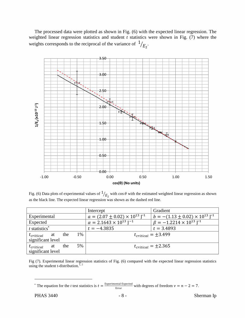
The processed data were plotted as shown in Fig. (6) with the expected linear regression. The
weighted linear regression statistics and student t statistics were shown in Fig. (7) where the
weights corresponds to the reciprocal of the variance of ⁄ .
Fig. (6) Data plots of experimental values of
⁄ with with the estimated weighted linear regression as shown
as the black line. The expected linear regression was shown as the dashed red line.
Intercept Gradient
Experimental Expected
t statistics
at the 1%
significant level
at the 5%
significant level
Fig (7). Experimental linear regression statistics of Fig. (6) compared with the expected linear regression statistics
using the student t-distribution.1, 2
The equation for the t test statistics is
-
with degrees of freedom .
0.00
0.50
1.00
1.50
2.00
2.50
3.00
3.50
-1.00 -0.50 0.00 0.50 1.00 1.50
1/E
2 (x
10
-13
J-1)
cos(θ) (No units)

PHAS 3440 - 9 - Sherman Ip
From observations of Fig. (6), it was possible to state that the expected linear regression is
quite different from the experimental linear regression because they are not parallel and the
intercepts have about an error bar difference. The student t statistics were compared for the
gradient and intercept with the expected values in Fig. (7). Following from the comparison, there
was evidence at the 1% significant level that the experimental intercept was significantly
different from expectation, but there was no evidence at the 1% significant level that the
experimental gradient was significantly different from expectation.1 This was quite unusual
considering Fig. (8) showed evidence the model fitted the experimental data but the processed
data found the intercept was significantly different from expectation. This suggested there may
be a systematic error.
Eq. (11) and Eq. (12) were used to obtain an experimental electron mass of . The 99% confidence limits
was worked out to be . The 99%
confidence level was used because the experimental data appeared to be significantly different
from expected, therefore more room for error was allowed. The 99% confidence interval does
not contain the expected electron mass of , therefore there was evidence at the
1% significant level that the mean experimental electron mass was different from the expected
electron mass.1, 3
From Fig. (7) there was evidence that the magnitude of the intercept and gradient was an
underestimate. By considering Eq. (11), this would implied the experimental electron mass will
be an overestimate, which was consistent with the experimental data.
Eq. (6) suggested readings of the energy of the scattered photons were an overestimate. A
closer look at Fig. (5) revealed most of the experimental data were slightly over the model as
shown as the black curve. This was evidence that the readings of the energy of the scattered
photon were an overestimate, causing a systematic error. The data is real so only the model can
be adjusted. The model Eq. (5) was modified to Eq. (13) to consider the systematic error.
[
]
(13)(offset error )
The offset error was estimated to be about +10.2 keV because this value of minimized .
The new model Eq. (13) was plotted as the blue curve with the experimental data in Fig. (5). The
test statistics were compared to show which model, Eq. (5) or Eq. (13), fitted with the
experimental data better as shown in Fig. (8).
Model Eq. (5) (No offset) Eq. (10) (Includes offset)
11.28 3.48
8† 7
‡
at the 5% significant level 15.51 14.07
18% 84% Fig. (8) statistics were compared for model Eq. (5) and Eq. (13).
The 99% confidence limits was obtained by combining the 99% confidence limits of , , and using Eq.
(11) and Eq. (12). † The degrees of freedom for the distribution is because there are 9 data points but one degree of
freedom must be lost because the number of data points is fixed at 9.1
‡ The degrees of freedom for the distribution is because there are 9 data points but two degree of
freedom were lost because the number of data points is fixed at 9 and was estimated by mininising .1
PHAS 3440 - 10 - Sherman Ip
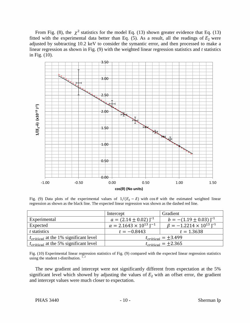
From Fig. (8), the statistics for the model Eq. (13) shown greater evidence that Eq. (13)
fitted with the experimental data better than Eq. (5). As a result, all the readings of were
adjusted by subtracting 10.2 keV to consider the symantic error, and then processed to make a
linear regression as shown in Fig. (9) with the weighted linear regression statistics and t statistics
in Fig. (10).
Fig. (9) Data plots of the experimental values of ⁄ with with the estimated weighted linear
regression as shown as the black line. The expected linear regression was shown as the dashed red line.
Intercept Gradient
Experimental Expected t statistics
at the 1% significant level
at the 5% significant level
Fig. (10) Experimental linear regression statistics of Fig. (9) compared with the expected linear regression statistics
using the student t-distribution. 1, 2
The new gradient and intercept were not significantly different from expectation at the 5%
significant level which showed by adjusting the values of with an offset error, the gradient
and intercept values were much closer to expectation.
0.00
0.50
1.00
1.50
2.00
2.50
3.00
3.50
-1.00 -0.50 0.00 0.50 1.00 1.50
1/(
E 2-δ
) (x
10
-13
J-1)
cos(θ) (No units)

PHAS 3440 - 11 - Sherman Ip
The gradient and intercept were used with Eq. (11) and Eq. (12) to obtain an electron mass of
and the 99% confidence limits of the electron mass was . The experimental value of the electron mass was certainly closer to the expected value
but the 99% confidence interval still does not contain the expected electron mass, of . This implied there was evidence the experimental electron mass was still significantly
different from the expected electron mass at the 1% significance level.1
V. CONCLUSION
Strong evidence was obtained that Eq. (5) and Eq. (13) fitted with the experimental data,
showing that the photon energies changes according to the Compton Effect.
By noticing a systematic error, the electron mass was obtained with mean and standard
deviation shown below.
The 99% confidence limits of the mean experimental electron mass was shown below.
⟨ ̅⟩ .
The 99% confidence interval does not contain the expected electron mass, shown below to 3
significant figures, this was evidence the mean experimental electron mass was significantly
different from the expected electron mass.3
The cause of systematic error was very likely from the energy calibration of the scintillation
counter, only Cs-137 was used for calibration which can be unreliable. More radioactive sources
should be used for calibration to increase the accuracy of the readings of energy.
The peaks interpreted from Figs. (4) was fine but the peaks may become undistinguishable at
small angles and angles approaching 180°. For high angles, the energies of the scattered photons
will have around the same magnitude of background radiation. In Fig. (4i), the two energy peaks
(background radiation and scattered photon energy) were back to back which may interfere with
the Cassy Lab Normal curve fit. Same implied in Fig. (4b) where the two energy peaks (direct
photon energy and scattered photon energy) ware back to back. The experiment can be improved
if nuisance energy peaks were removed by completely shielding the photon or scattering path
and shielding the experiment to prevent the scintillation counter absorbing background radiation.
VI. REFERENCES
1. Davies, M., Dunnett, R., Eccles, A., Green, N., & Porkess, R. (2005). Statistics 3 (3rd ed.).
Hodder Education.
2. Davies, M., Eccles, A., Francis, B., Green, N., & Porkess, R. (2005). Statistics 2 (3rd ed.).
Hodder Education.
3. Littlefield, T. A., & Thorley, N. (1979). Atomic and Nuclear Physics (3rd ed.). Van Nostrand
Reinhold Co. Ltd.
4. Rae, A. I. (2008). Quantum Mechanics (5th ed.). Taylor & Francis Group.
Top Related