


Languages
Pages
Legal


Compilation 0368-3133 (Semester A, 2013/14)
Lecture 11: Data Flow Analysis & Optimizations
Noam Rinetzky
Slides credit: Roman Manevich, Mooly Sagiv and Eran Yahav
2
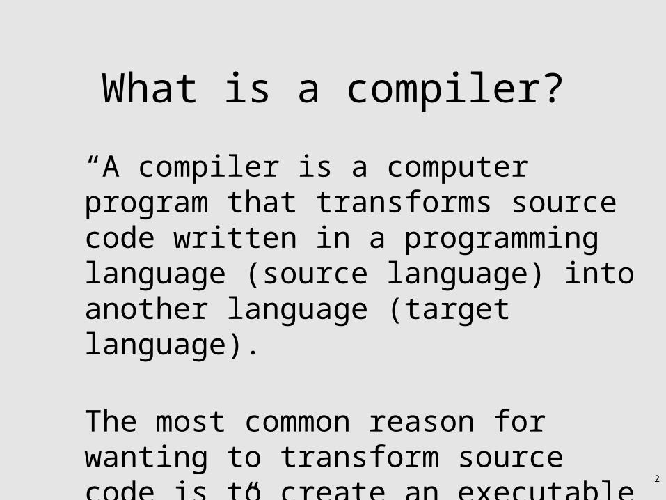
What is a compiler?
“A compiler is a computer program that transforms source code written in a programming language (source language) into another language (target language).
The most common reason for wanting to transform source code is to create an executable program.”
--Wikipedia

3
AST
+ Sy
m. T
ab.
Stages of compilationSource code
(program)
LexicalAnalysis
Syntax Analysis
Parsing
Context Analysis
Portable/Retargetable
code generation
Target code
(executable)
Asse
mbl
y
IRText
Toke
n st
ream
AST
CodeGeneration
4
Inst
ructi
on s
elec
tion
AST
+ Sy
m. T
ab.
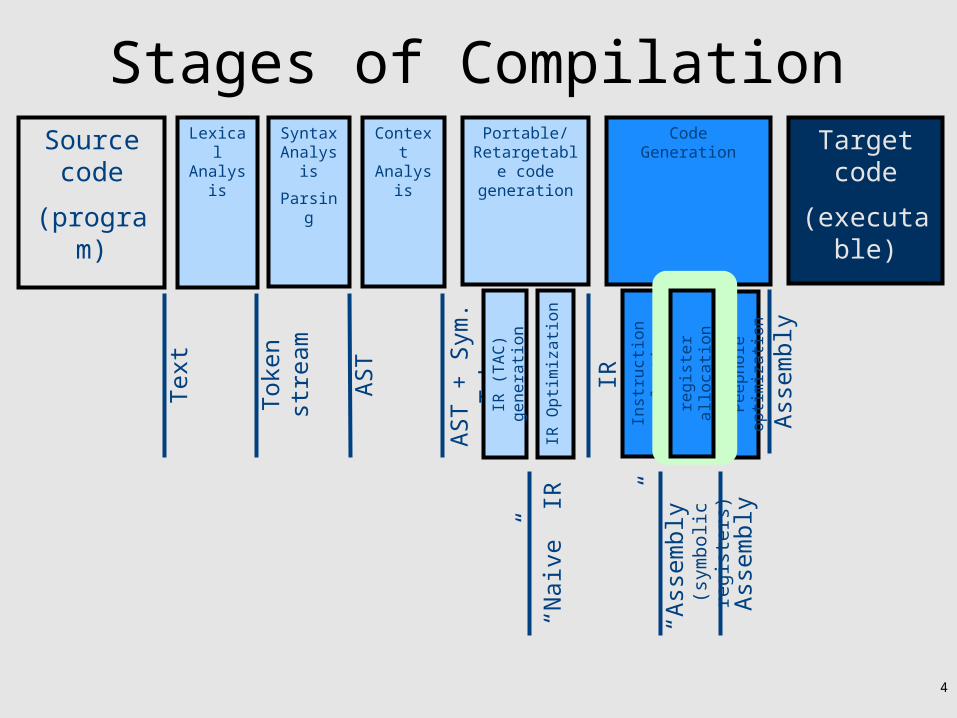
Stages of CompilationSource code
(program)
LexicalAnalysis
Syntax Analysis
Parsing
Context Analysis
Portable/Retargetable
code generation
Target code
(executable)
Asse
mbl
y
IRText
Toke
n st
ream
AST
“Nai
ve”
IRIR
Opti
miza
tion
IR (T
AC) g
ener
ation
“Ass
embl
y”
(sym
bolic
regi
ster
s)
Peep
hole
opti
miza
tion
Asse
mbl
y
CodeGeneration
regi
ster
allo
catio
n

Registers
• Most machines have a set of registers, dedicated memory locations that– can be accessed quickly,– can have computations performed on them, and– are used for special purposes (e.g., parameter passing)
• Usages– Operands of instructions– Store temporary results– Can (should) be used as loop indexes due to frequent
arithmetic operation – Used to manage administrative info
• e.g., runtime stack

Register Allocation
• Machine-agnostic optimizations• Assume unbounded number of registers
– Expression trees (tree-local)– Basic blocks (block-local)
• Machine-dependent optimization• K registers• Some have special purposes
– Control flow graphs (global register allocation)

Register Allocation for Expression trees
*
b b1 1
2 -
*
4 *
a c1 1
21
2
2
t71
t7 := b * b x := t7 – 4 * a * c
x := b*b-4*a*c
?

Register Allocation for Basic Blocks
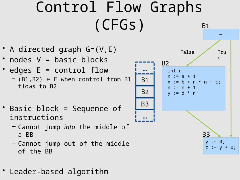
Control Flow Graphs (CFGs)
• A directed graph G=(V,E)• nodes V = basic blocks• edges E = control flow
– (B1,B2) E when control from B1 flows to B2
• Basic block = Sequence of instructions– Cannot jump into the middle of a BB– Cannot jump out of the middle of
the BB
• Leader-based algorithm
B1
B2
…
… int n; n := a + 1; x := b + n * n + c; n := n + 1; y := d * n;
y := 0; z := y + x;
False True
…
B3
B1
B2
B3

y, dead or alive?
int n; n := a + 1; x := b + n * n + c; n := n + 1; y := d * n;
y := 0; z := y + x;
False True
…
int n; n := a + 1; x := b + n * n + c; n := n + 1; y := d * n;
z := y + x; y := 0;
False True
…

Variable Liveness
• A statement x = y + z– defines x– uses y and z
• A variable x is live at a program point if its value (at this point) is used at a later point
y = 42z = 73x = y + zprint(x);
x is live, y dead, z deadx undef, y live, z livex undef, y live, z undef
x is dead, y dead, z dead
(showing state after the statement)

Global Register Allocation using Liveness Information
• For every node n in CFG, we have out[n]– Set of temporaries live out of n
• Two variables interfere if they appear in the same out[n] of any node n– Cannot be allocated to the same register
• Conversely, if two variables do not interfere with each other, they can be assigned the same register– We say they have disjoint live ranges
• How to assign registers to variables?

Interference graph Callee-saved registers
Caller-saved registers
R1,r2 pass parametersR1 stores return
value

14
Optimization points
sourcecode
Frontend IR
Codegenerator
targetcode
Userprofile program
change algorithm
Compilerintraprocedural IRInterprocedural IRIR optimizations
Compilerregister allocation
instruction selectionpeephole transformations
today
15
Program Analysis
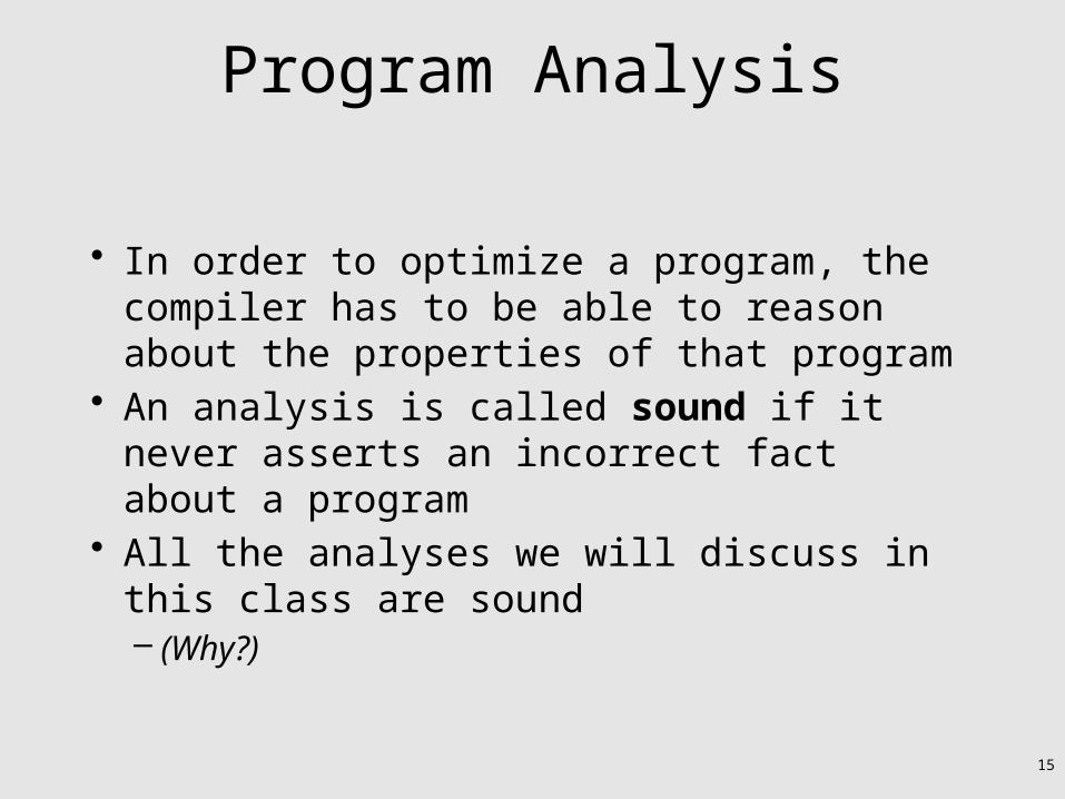
• In order to optimize a program, the compiler has to be able to reason about the properties of that program
• An analysis is called sound if it never asserts an incorrect fact about a program
• All the analyses we will discuss in this class are sound– (Why?)

16
Soundness
int x;int y;
if (y < 5) x = 137;else x = 42;
Print(x);
“At this point in theprogram, x holds some
integer value”

17
Soundness
int x;int y;
if (y < 5) x = 137;else x = 42;
Print(x);
“At this point in theprogram, x is either 137 or 42”
18
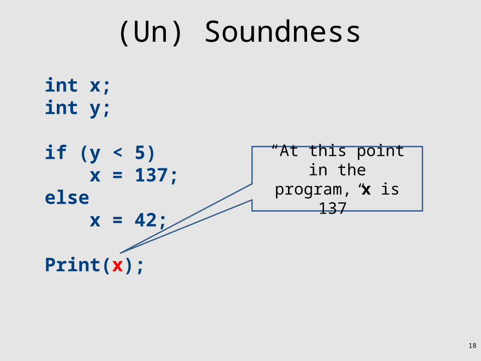
(Un) Soundness
int x;int y;
if (y < 5) x = 137;else x = 42;
Print(x);
“At this point in theprogram, x is 137”
19
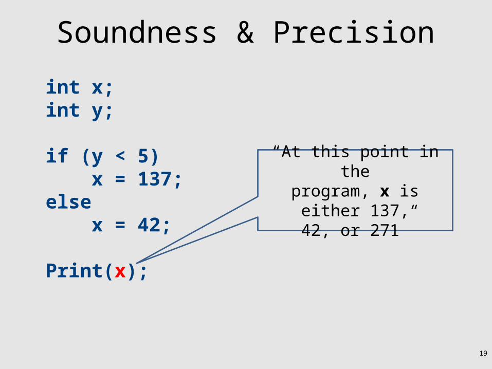
Soundness & Precision
int x;int y;
if (y < 5) x = 137;else x = 42;
Print(x);
“At this point in theprogram, x is either 137,
42, or 271”

20
Semantics-preserving optimizations
• An optimization is semantics-preserving if it does not alter the semantics (meaning) of the original programEliminating unnecessary temporary variablesComputing values that are known statically at compile-
time instead of computing them at runtimeEvaluating iteration-independent expressions outside
of a loop instead of inside✗Replacing bubble sort with quicksort (why?)
• The optimizations we will consider in this class are all semantics-preserving

21
A formalism for IR optimization
• Every phase of the compiler uses some new abstraction:– Scanning uses regular expressions– Parsing uses Context Free Grammars (CFGs)– Semantic analysis uses proof systems and symbol tables– IR generation uses ASTs
• In optimization, we need a formalism that captures the structure of a program in a way amenable to optimization– Control Flow Graphs (CFGs)

22
Types of optimizations
• An optimization is local if it works on just a single basic block
• An optimization is global if it works on an entire control-flow graph
• An optimization is interprocedural if it works across the control-flow graphs of multiple functions– We won't talk about this in this course

23
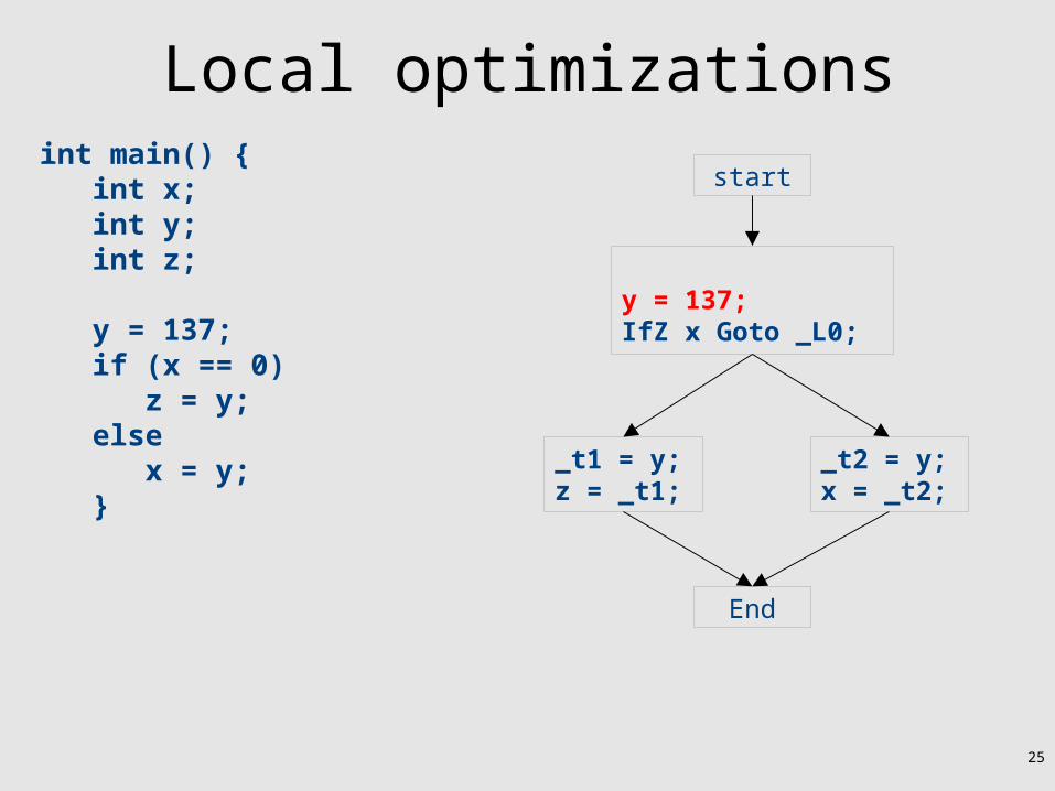
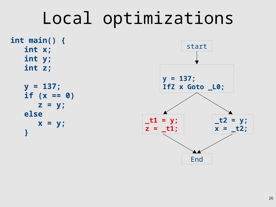
Local optimizations
_t0 = 137;y = _t0;IfZ x Goto _L0;
start
_t1 = y;z = _t1;
_t2 = y;x = _t2;
start
int main() {int x;int y;int z;
y = 137;if (x == 0)
z = y;else
x = y;}

24
Local optimizations
_t0 = 137;y = _t0;IfZ x Goto _L0;
start
_t1 = y;z = _t1;
_t2 = y;x = _t2;
End
int main() {int x;int y;int z;
y = 137;if (x == 0)
z = y;else
x = y;}
25
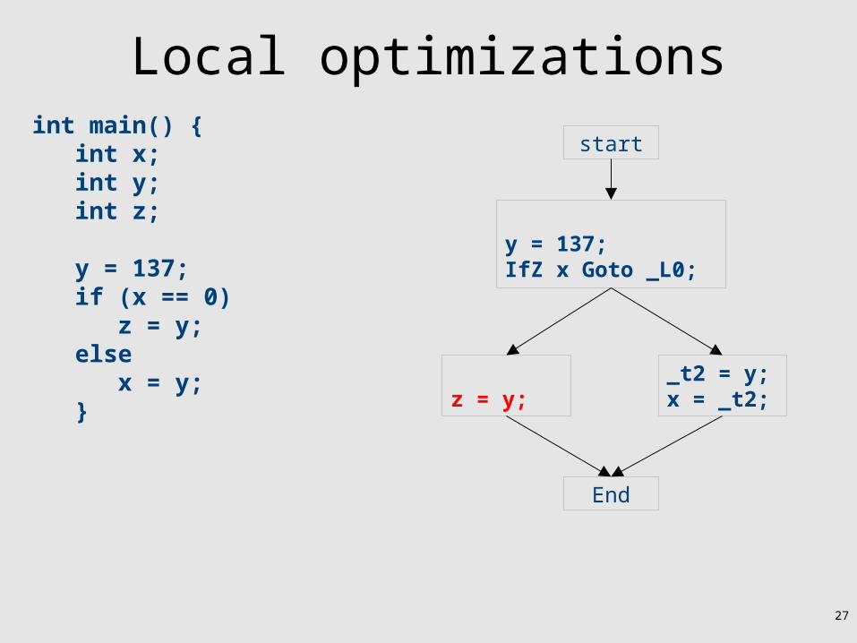
Local optimizations
y = 137;IfZ x Goto _L0;
start
_t1 = y;z = _t1;
_t2 = y;x = _t2;
End
int main() {int x;int y;int z;
y = 137;if (x == 0)
z = y;else
x = y;}
26
Local optimizations
y = 137;IfZ x Goto _L0;
start
_t1 = y;z = _t1;
_t2 = y;x = _t2;
End
int main() {int x;int y;int z;
y = 137;if (x == 0)
z = y;else
x = y;}
27
Local optimizations
y = 137;IfZ x Goto _L0;
start
z = y;_t2 = y;x = _t2;
End
int main() {int x;int y;int z;
y = 137;if (x == 0)
z = y;else
x = y;}

28
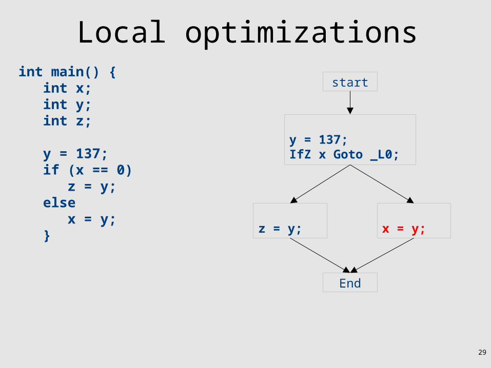
Local optimizations
y = 137;IfZ x Goto _L0;
start
z = y;_t2 = y;x = _t2;
End
int main() {int x;int y;int z;
y = 137;if (x == 0)
z = y;else
x = y;}
29
Local optimizations
y = 137;IfZ x Goto _L0;
start
z = y; x = y;
End
int main() {int x;int y;int z;
y = 137;if (x == 0)
z = y;else
x = y;}

30
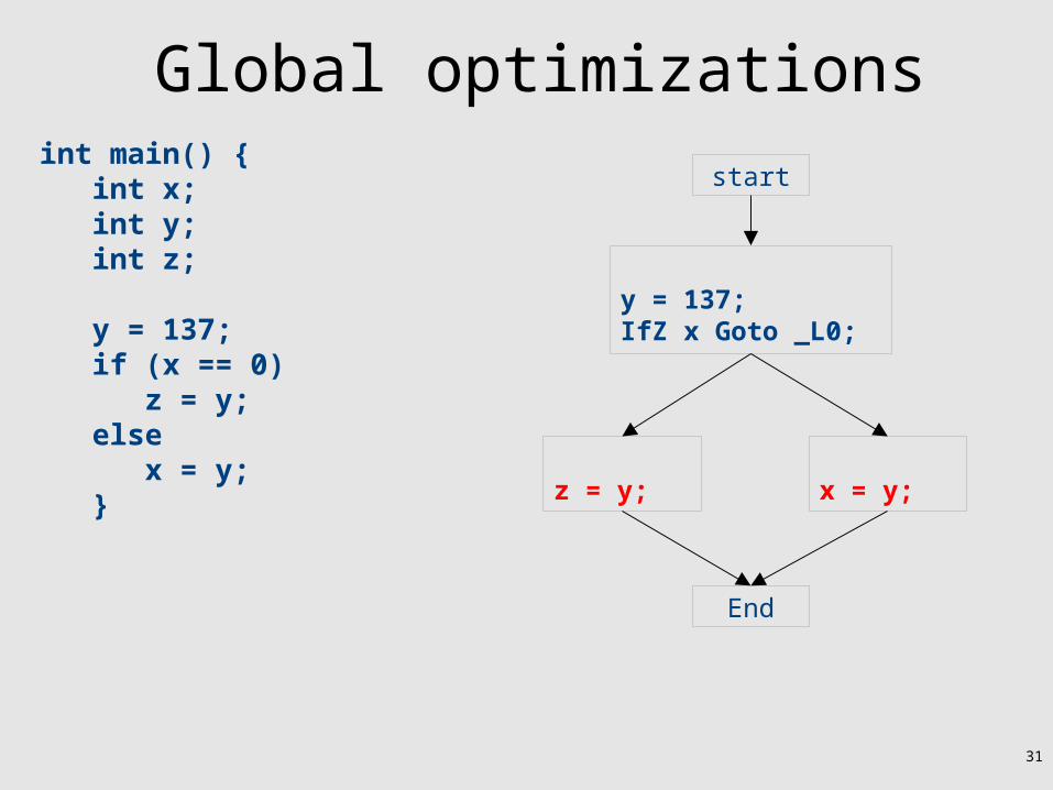
Global optimizations
y = 137;IfZ x Goto _L0;
start
z = y; x = y;
End
int main() {int x;int y;int z;
y = 137;if (x == 0)
z = y;else
x = y;}
31
Global optimizations
y = 137;IfZ x Goto _L0;
start
z = y; x = y;
End
int main() {int x;int y;int z;
y = 137;if (x == 0)
z = y;else
x = y;}

32
Global optimizations
y = 137;IfZ x Goto _L0;
start
z = 137; x = 137;
End
int main() {int x;int y;int z;
y = 137;if (x == 0)
z = y;else
x = y;}

33
Local Optimizations

34
Optimization path
IR Control-FlowGraph
CFGbuilder
ProgramAnalysis
AnnotatedCFG
OptimizingTransformation
TargetCode
CodeGeneration
(+optimizations)
donewith IR
optimizations
IRoptimizations

35
Common subexpression eliminationObject x;int a;int b;int c;
x = new Object;a = 4;c = a + b;x.fn(a + b);
_tmp0 = 4;Push _tmp0;_tmp1 = Call _Alloc;Pop tmp2;*(_tmp1) = _tmp2;x = _tmp1;_tmp3 = 4;a = _tmp3;_tmp4 = a + b;c = _tmp4;_tmp5 = a + b;_tmp6 = *(x);_tmp7 = *(_tmp6);Push _tmp5;Push x;Call _tmp7;

36
Common subexpression eliminationObject x;int a;int b;int c;
x = new Object;a = 4;c = a + b;x.fn(a + b);
_tmp0 = 4;Push _tmp0;_tmp1 = Call _Alloc;Pop tmp2;*(_tmp1) = _tmp2;x = _tmp1;_tmp3 = 4;a = _tmp3;_tmp4 = a + b;c = _tmp4;_tmp5 = a + b;_tmp6 = *(x);_tmp7 = *(_tmp6);Push _tmp5;Push x;Call _tmp7;
37
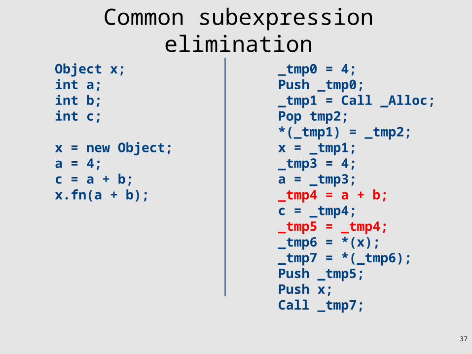
Common subexpression eliminationObject x;int a;int b;int c;
x = new Object;a = 4;c = a + b;x.fn(a + b);
_tmp0 = 4;Push _tmp0;_tmp1 = Call _Alloc;Pop tmp2;*(_tmp1) = _tmp2;x = _tmp1;_tmp3 = 4;a = _tmp3;_tmp4 = a + b;c = _tmp4;_tmp5 = _tmp4;_tmp6 = *(x);_tmp7 = *(_tmp6);Push _tmp5;Push x;Call _tmp7;

38
Common subexpression eliminationObject x;int a;int b;int c;
x = new Object;a = 4;c = a + b;x.fn(a + b);
_tmp0 = 4;Push _tmp0;_tmp1 = Call _Alloc;Pop tmp2;*(_tmp1) = _tmp2;x = _tmp1;_tmp3 = 4;a = _tmp3;_tmp4 = a + b;c = _tmp4;_tmp5 = _tmp4;_tmp6 = *(x);_tmp7 = *(_tmp6);Push _tmp5;Push x;Call _tmp7;

39
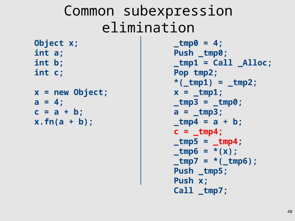
Common subexpression eliminationObject x;int a;int b;int c;
x = new Object;a = 4;c = a + b;x.fn(a + b);
_tmp0 = 4;Push _tmp0;_tmp1 = Call _Alloc;Pop tmp2;*(_tmp1) = _tmp2;x = _tmp1;_tmp3 = _tmp0;a = _tmp3;_tmp4 = a + b;c = _tmp4;_tmp5 = _tmp4;_tmp6 = *(x);_tmp7 = *(_tmp6);Push _tmp5;Push x;Call _tmp7;
40
Common subexpression eliminationObject x;int a;int b;int c;
x = new Object;a = 4;c = a + b;x.fn(a + b);
_tmp0 = 4;Push _tmp0;_tmp1 = Call _Alloc;Pop tmp2;*(_tmp1) = _tmp2;x = _tmp1;_tmp3 = _tmp0;a = _tmp3;_tmp4 = a + b;c = _tmp4;_tmp5 = _tmp4;_tmp6 = *(x);_tmp7 = *(_tmp6);Push _tmp5;Push x;Call _tmp7;

41
Common subexpression eliminationObject x;int a;int b;int c;
x = new Object;a = 4;c = a + b;x.fn(a + b);
_tmp0 = 4;Push _tmp0;_tmp1 = Call _Alloc;Pop tmp2;*(_tmp1) = _tmp2;x = _tmp1;_tmp3 = _tmp0;a = _tmp3;_tmp4 = a + b;c = _tmp4;_tmp5 = c;_tmp6 = *(x);_tmp7 = *(_tmp6);Push _tmp5;Push x;Call _tmp7;
42
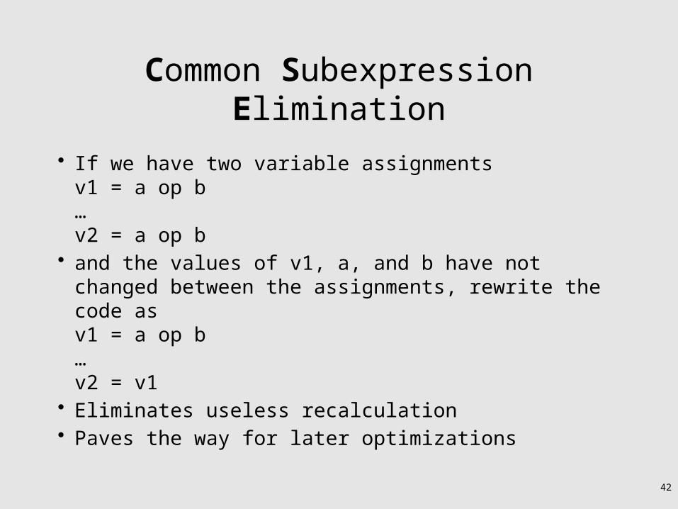
Common Subexpression Elimination
• If we have two variable assignmentsv1 = a op b…v2 = a op b
• and the values of v1, a, and b have not changed between the assignments, rewrite the code asv1 = a op b…v2 = v1
• Eliminates useless recalculation• Paves the way for later optimizations

43
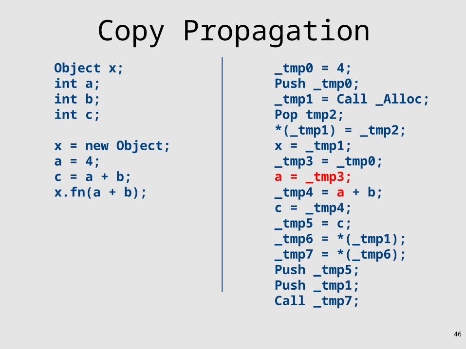
Copy PropagationObject x;int a;int b;int c;
x = new Object;a = 4;c = a + b;x.fn(a + b);
_tmp0 = 4;Push _tmp0;_tmp1 = Call _Alloc;Pop tmp2;*(_tmp1) = _tmp2;x = _tmp1;_tmp3 = _tmp0;a = _tmp3;_tmp4 = a + b;c = _tmp4;_tmp5 = c;_tmp6 = *(x);_tmp7 = *(_tmp6);Push _tmp5;Push x;Call _tmp7;

44
Copy PropagationObject x;int a;int b;int c;
x = new Object;a = 4;c = a + b;x.fn(a + b);
_tmp0 = 4;Push _tmp0;_tmp1 = Call _Alloc;Pop tmp2;*(_tmp1) = _tmp2;x = _tmp1;_tmp3 = _tmp0;a = _tmp3;_tmp4 = a + b;c = _tmp4;_tmp5 = c;_tmp6 = *(x);_tmp7 = *(_tmp6);Push _tmp5;Push x;Call _tmp7;

45
Copy PropagationObject x;int a;int b;int c;
x = new Object;a = 4;c = a + b;x.fn(a + b);
_tmp0 = 4;Push _tmp0;_tmp1 = Call _Alloc;Pop tmp2;*(_tmp1) = _tmp2;x = _tmp1;_tmp3 = _tmp0;a = _tmp3;_tmp4 = a + b;c = _tmp4;_tmp5 = c;_tmp6 = *(_tmp1);_tmp7 = *(_tmp6);Push _tmp5;Push _tmp1;Call _tmp7;
46
Copy PropagationObject x;int a;int b;int c;
x = new Object;a = 4;c = a + b;x.fn(a + b);
_tmp0 = 4;Push _tmp0;_tmp1 = Call _Alloc;Pop tmp2;*(_tmp1) = _tmp2;x = _tmp1;_tmp3 = _tmp0;a = _tmp3;_tmp4 = a + b;c = _tmp4;_tmp5 = c;_tmp6 = *(_tmp1);_tmp7 = *(_tmp6);Push _tmp5;Push _tmp1;Call _tmp7;

47
Copy PropagationObject x;int a;int b;int c;
x = new Object;a = 4;c = a + b;x.fn(a + b);
_tmp0 = 4;Push _tmp0;_tmp1 = Call _Alloc;Pop tmp2;*(_tmp1) = _tmp2;x = _tmp1;_tmp3 = _tmp0;a = _tmp3;_tmp4 = _tmp3 + b;c = _tmp4;_tmp5 = c;_tmp6 = *(_tmp1);_tmp7 = *(_tmp6);Push _tmp5;Push _tmp1;Call _tmp7;

48
Copy PropagationObject x;int a;int b;int c;
x = new Object;a = 4;c = a + b;x.fn(a + b);
_tmp0 = 4;Push _tmp0;_tmp1 = Call _Alloc;Pop tmp2;*(_tmp1) = _tmp2;x = _tmp1;_tmp3 = _tmp0;a = _tmp3;_tmp4 = _tmp3 + b;c = _tmp4;_tmp5 = c;_tmp6 = *(_tmp1);_tmp7 = *(_tmp6);Push _tmp5;Push _tmp1;Call _tmp7;

49
Copy PropagationObject x;int a;int b;int c;
x = new Object;a = 4;c = a + b;x.fn(a + b);
_tmp0 = 4;Push _tmp0;_tmp1 = Call _Alloc;Pop tmp2;*(_tmp1) = _tmp2;x = _tmp1;_tmp3 = _tmp0;a = _tmp3;_tmp4 = _tmp3 + b;c = _tmp4;_tmp5 = c;_tmp6 = *(_tmp1);_tmp7 = *(_tmp6);Push c;Push _tmp1;Call _tmp7;

50
Copy PropagationObject x;int a;int b;int c;
x = new Object;a = 4;c = a + b;x.fn(a + b);
_tmp0 = 4;Push _tmp0;_tmp1 = Call _Alloc;Pop tmp2;*(_tmp1) = _tmp2;x = _tmp1;_tmp3 = _tmp0;a = _tmp3;_tmp4 = _tmp3 + b;c = _tmp4;_tmp5 = c;_tmp6 = *(_tmp1);_tmp7 = *(_tmp6);Push c;Push _tmp1;Call _tmp7;

51
Copy PropagationObject x;int a;int b;int c;
x = new Object;a = 4;c = a + b;x.fn(a + b);
_tmp0 = 4;Push _tmp0;_tmp1 = Call _Alloc;Pop tmp2;*(_tmp1) = _tmp2;x = _tmp1;_tmp3 = _tmp0;a = _tmp3;_tmp4 = _tmp3 + b;c = _tmp4;_tmp5 = c;_tmp6 = _tmp2;_tmp7 = *(_tmp6);Push c;Push _tmp1;Call _tmp7;
52
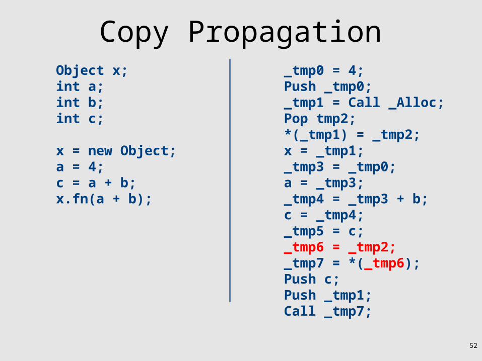
Copy PropagationObject x;int a;int b;int c;
x = new Object;a = 4;c = a + b;x.fn(a + b);
_tmp0 = 4;Push _tmp0;_tmp1 = Call _Alloc;Pop tmp2;*(_tmp1) = _tmp2;x = _tmp1;_tmp3 = _tmp0;a = _tmp3;_tmp4 = _tmp3 + b;c = _tmp4;_tmp5 = c;_tmp6 = _tmp2;_tmp7 = *(_tmp6);Push c;Push _tmp1;Call _tmp7;

53
Copy PropagationObject x;int a;int b;int c;
x = new Object;a = 4;c = a + b;x.fn(a + b);
_tmp0 = 4;Push _tmp0;_tmp1 = Call _Alloc;Pop tmp2;*(_tmp1) = _tmp2;x = _tmp1;_tmp3 = _tmp0;a = _tmp3;_tmp4 = _tmp3 + b;c = _tmp4;_tmp5 = c;_tmp6 = _tmp2;_tmp7 = *(_tmp2);Push c;Push _tmp1;Call _tmp7;

54
Copy Propagation_tmp0 = 4;Push _tmp0;_tmp1 = Call _Alloc;Pop tmp2;*(_tmp1) = _tmp2;x = _tmp1;_tmp3 = _tmp0;a = _tmp3;_tmp4 = _tmp3 + b;c = _tmp4;_tmp5 = c;_tmp6 = _tmp2;_tmp7 = *(_tmp2);Push c;Push _tmp1;Call _tmp7;
Object x;int a;int b;int c;
x = new Object;a = 4;c = a + b;x.fn(a + b);

55
Copy Propagation_tmp0 = 4;Push _tmp0;_tmp1 = Call _Alloc;Pop tmp2;*(_tmp1) = _tmp2;x = _tmp1;_tmp3 = _tmp0;a = _tmp0;_tmp4 = _tmp0 + b;c = _tmp4;_tmp5 = c;_tmp6 = _tmp2;_tmp7 = *(_tmp2);Push c;Push _tmp1;Call _tmp7;
56
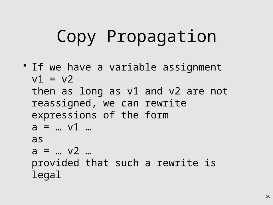
Copy Propagation
• If we have a variable assignmentv1 = v2then as long as v1 and v2 are not reassigned, we can rewrite expressions of the forma = … v1 …asa = … v2 …provided that such a rewrite is legal
57
Dead Code EliminationObject x;int a;int b;int c;
x = new Object;a = 4;c = a + b;x.fn(a + b);
_tmp0 = 4;Push _tmp0;_tmp1 = Call _Alloc;Pop tmp2;*(_tmp1) = _tmp2;x = _tmp1;_tmp3 = _tmp0;a = _tmp0;_tmp4 = _tmp0 + b;c = _tmp4;_tmp5 = c;_tmp6 = _tmp2;_tmp7 = *(_tmp2);Push c;Push _tmp1;Call _tmp7;

58
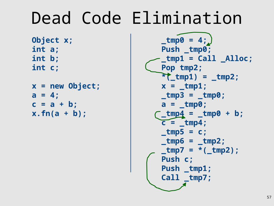
Dead Code EliminationObject x;int a;int b;int c;
x = new Object;a = 4;c = a + b;x.fn(a + b);
_tmp0 = 4;Push _tmp0;_tmp1 = Call _Alloc;Pop tmp2;*(_tmp1) = _tmp2;x = _tmp1;_tmp3 = _tmp0;a = _tmp0;_tmp4 = _tmp0 + b;c = _tmp4;_tmp5 = c;_tmp6 = _tmp2;_tmp7 = *(_tmp2);Push c;Push _tmp1;Call _tmp7;
values never read
values never read
59
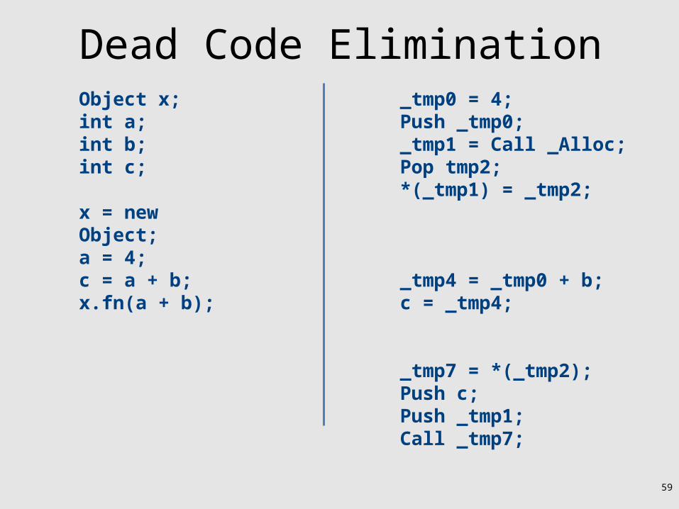
Dead Code EliminationObject x;int a;int b;int c;
x = new Object;a = 4;c = a + b;x.fn(a + b);
_tmp0 = 4;Push _tmp0;_tmp1 = Call _Alloc;Pop tmp2;*(_tmp1) = _tmp2;
_tmp4 = _tmp0 + b;c = _tmp4;
_tmp7 = *(_tmp2);Push c;Push _tmp1;Call _tmp7;
60
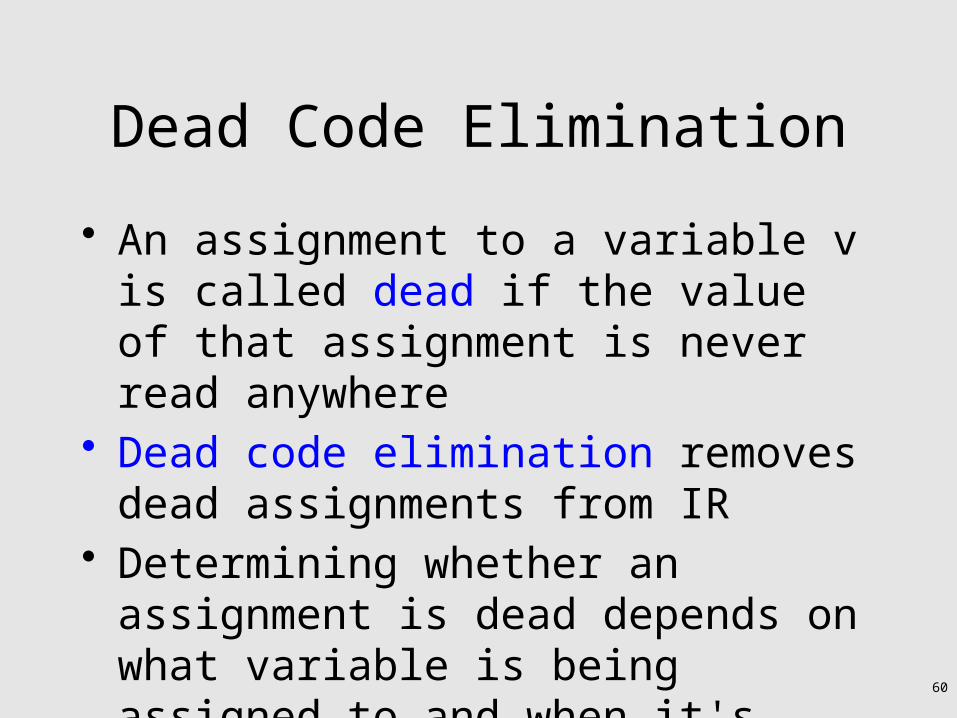
Dead Code Elimination
• An assignment to a variable v is called dead if the value of that assignment is never read anywhere
• Dead code elimination removes dead assignments from IR
• Determining whether an assignment is dead depends on what variable is being assigned to and when it's being assigned
61
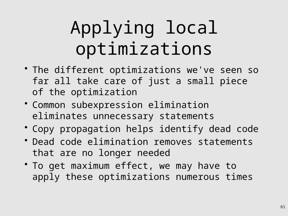
Applying local optimizations
• The different optimizations we've seen so far all take care of just a small piece of the optimization
• Common subexpression elimination eliminates unnecessary statements
• Copy propagation helps identify dead code• Dead code elimination removes statements that
are no longer needed• To get maximum effect, we may have to apply
these optimizations numerous times
62
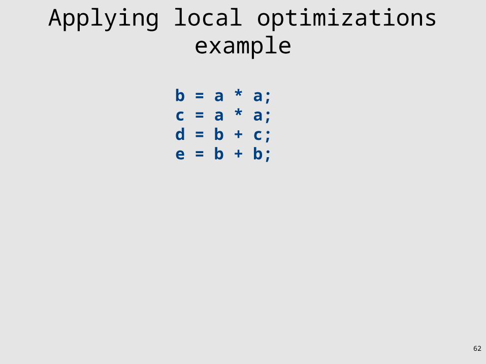
Applying local optimizations example
b = a * a;c = a * a;d = b + c;e = b + b;

63
Applying local optimizations example
b = a * a;c = a * a;d = b + c;e = b + b;
Which optimization should we apply here?

64
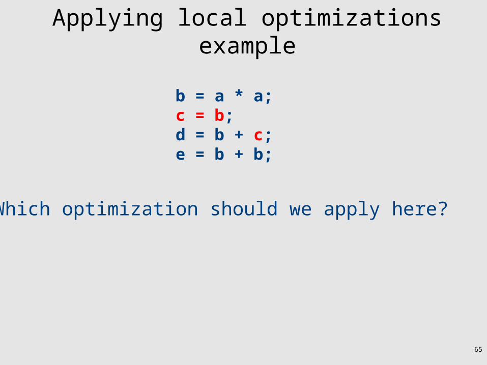
Applying local optimizations example
b = a * a;c = b;d = b + c;e = b + b;
Common sub-expression elimination
Which optimization should we apply here?
65
Applying local optimizations example
b = a * a;c = b;d = b + c;e = b + b;
Which optimization should we apply here?
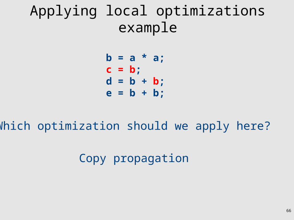
66
Applying local optimizations example
b = a * a;c = b;d = b + b;e = b + b;
Which optimization should we apply here?
Copy propagation

67
Applying local optimizations example
b = a * a;c = b;d = b + b;e = b + b;
Which optimization should we apply here?
68
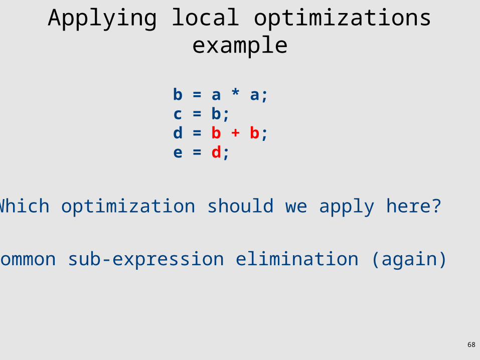
Applying local optimizations example
b = a * a;c = b;d = b + b;e = d;
Which optimization should we apply here?
Common sub-expression elimination (again)

69
Other types of local optimizations
• Arithmetic Simplification– Replace “hard” operations with easier ones– e.g. rewrite x = 4 * a; as x = a << 2;
• Constant Folding– Evaluate expressions at compile-time if they
have a constant value.– e.g. rewrite x = 4 * 5; as x = 20;

70
Optimizations and analyses
• Most optimizations are only possible given some analysis of the program's behavior
• In order to implement an optimization, we will talk about the corresponding program analyses

71
Available expressions
• Both common subexpression elimination and copy propagation depend on an analysis of the available expressions in a program
• An expression is called available if some variable in the program holds the value of that expression
• In common subexpression elimination, we replace an available expression by the variable holding its value
• In copy propagation, we replace the use of a variable by the available expression it holds
72
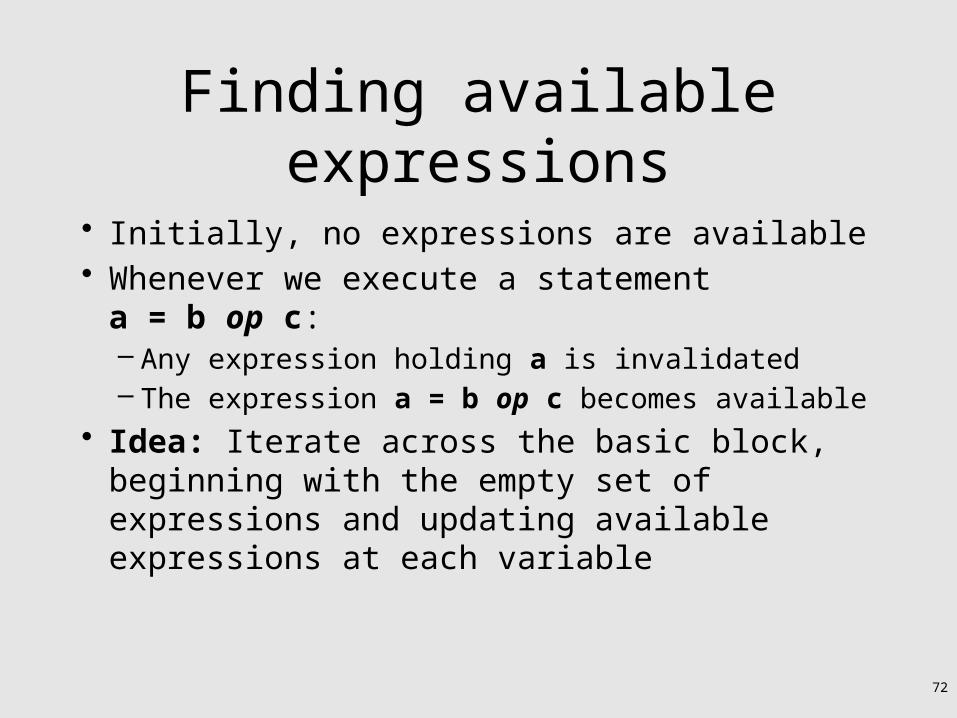
Finding available expressions
• Initially, no expressions are available• Whenever we execute a statement
a = b op c:– Any expression holding a is invalidated– The expression a = b op c becomes available
• Idea: Iterate across the basic block, beginning with the empty set of expressions and updating available expressions at each variable
73
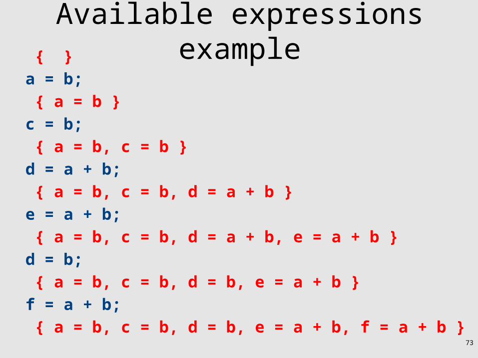
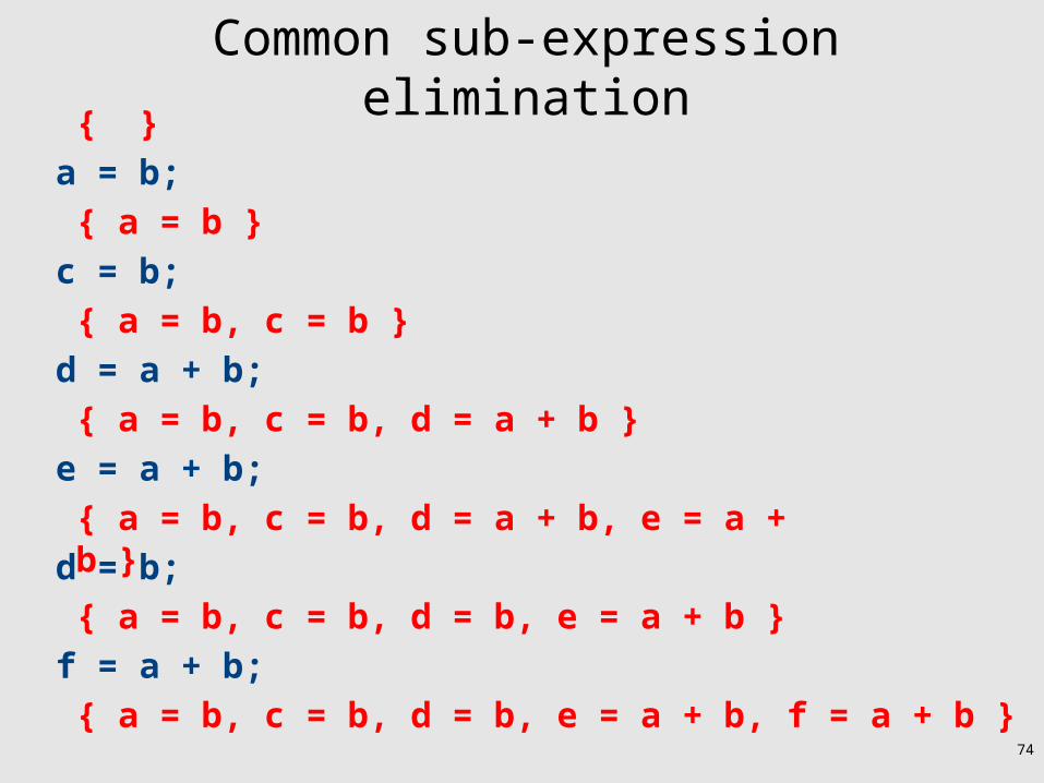
Available expressions examplea = b;
c = b;
d = a + b;
e = a + b;
d = b;
f = a + b;
{ a = b, c = b, d = b, e = a + b }
{ a = b, c = b, d = a + b, e = a + b }
{ a = b, c = b, d = a + b }
{ a = b, c = b }
{ a = b }
{ }
{ a = b, c = b, d = b, e = a + b, f = a + b }
74
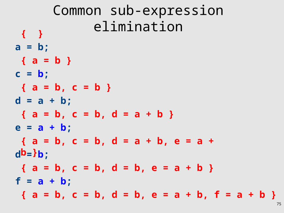
Common sub-expression elimination
a = b;
c = b;
d = a + b;
e = a + b;
d = b;
f = a + b;
{ a = b, c = b, d = b, e = a + b }
{ a = b, c = b, d = a + b, e = a + b }
{ a = b, c = b, d = a + b }
{ a = b, c = b }
{ a = b }
{ }
{ a = b, c = b, d = b, e = a + b, f = a + b }
75
Common sub-expression elimination
a = b;
c = b;
d = a + b;
e = a + b;
d = b;
f = a + b;
{ a = b, c = b, d = b, e = a + b }
{ a = b, c = b, d = a + b, e = a + b }
{ a = b, c = b, d = a + b }
{ a = b, c = b }
{ a = b }
{ }
{ a = b, c = b, d = b, e = a + b, f = a + b }

76
Common sub-expression elimination
a = b;
c = a;
d = a + b;
e = d;
d = a;
f = e;
{ a = b, c = b, d = b, e = a + b }
{ a = b, c = b, d = a + b, e = a + b }
{ a = b, c = b, d = a + b }
{ a = b, c = b }
{ a = b }
{ }
{ a = b, c = b, d = b, e = a + b, f = a + b }

77
Live variables
• The analysis corresponding to dead code elimination is called liveness analysis
• A variable is live at a point in a program if later in the program its value will be read before it is written to again
• Dead code elimination works by computing liveness for each variable, then eliminating assignments to dead variables

78
Computing live variables• To know if a variable will be used at some point,
we iterate across the statements in a basic block in reverse order
• Initially, some small set of values are known to be live (which ones depends on the particular program)
• When we see the statement a = b op c:– Just before the statement, a is not alive, since its value
is about to be overwritten– Just before the statement, both b and c are alive, since
we're about to read their values– (what if we have a = a + b?)
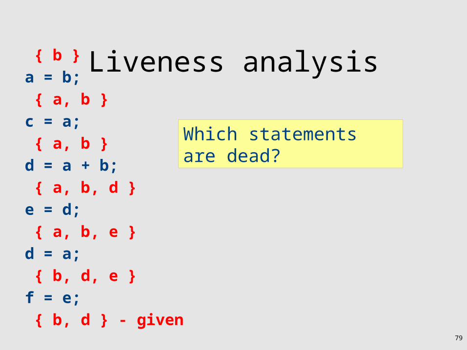
Liveness analysisa = b;
c = a;
d = a + b;
e = d;
d = a;
f = e;
{ b, d, e }
{ a, b, e }
{ a, b, d }
{ a, b }
{ a, b }
{ b }
{ b, d } - given
Which statements are dead?
79

Dead Code Eliminationa = b;
c = a;
d = a + b;
e = d;
d = a;
f = e;
{ b, d, e }
{ a, b, e }
{ a, b, d }
{ a, b }
{ a, b }
{ b }
{ b, d }
Which statements are dead?
80
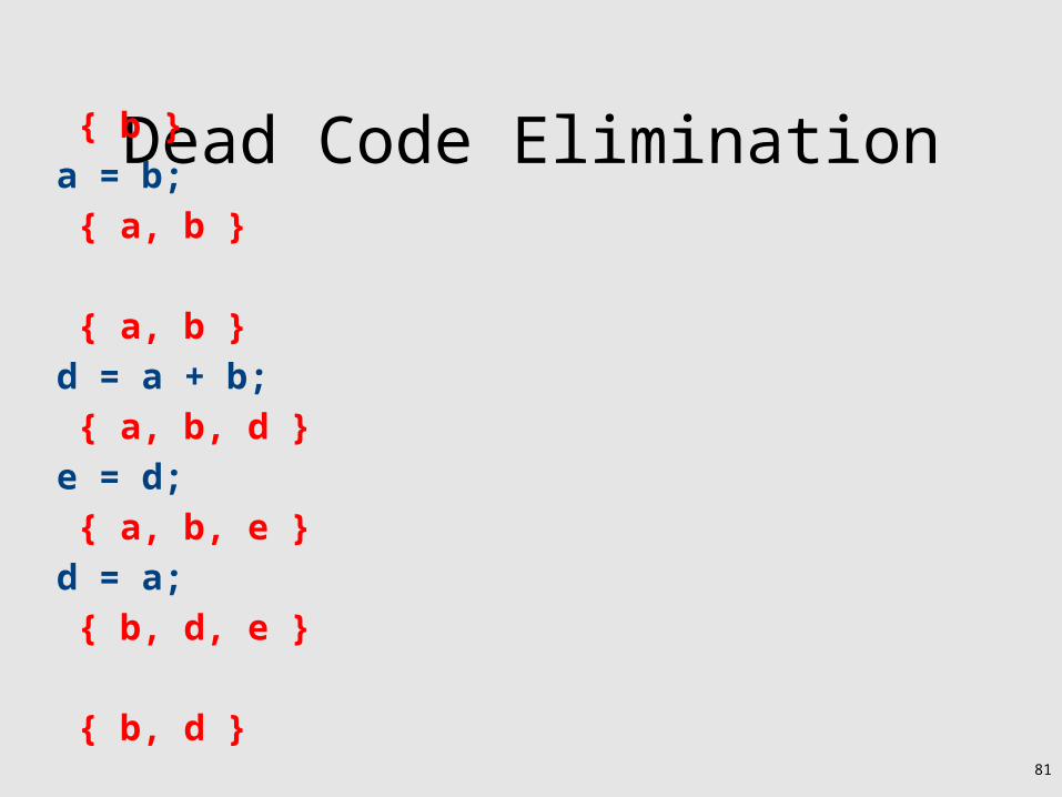
Dead Code Eliminationa = b;
d = a + b;
e = d;
d = a;
{ b, d, e }
{ a, b, e }
{ a, b, d }
{ a, b }
{ a, b }
{ b }
{ b, d }81

Liveness analysis IIa = b;
d = a + b;
e = d;
d = a;
{ b, d }
{ a, b }
{ a, b, d }
{ a, b }
{ b }
Which statements are dead?
82

Liveness analysis IIa = b;
d = a + b;
e = d;
d = a;
{ b, d }
{ a, b }
{ a, b, d }
{ a, b }
{ b }
Which statements are dead?
83

Dead code eliminationa = b;
d = a + b;
e = d;
d = a;
{ b, d }
{ a, b }
{ a, b, d }
{ a, b }
{ b }
Which statements are dead?
84

Dead code eliminationa = b;
d = a + b;
d = a;
{ b, d }
{ a, b }
{ a, b, d }
{ a, b }
{ b }
85
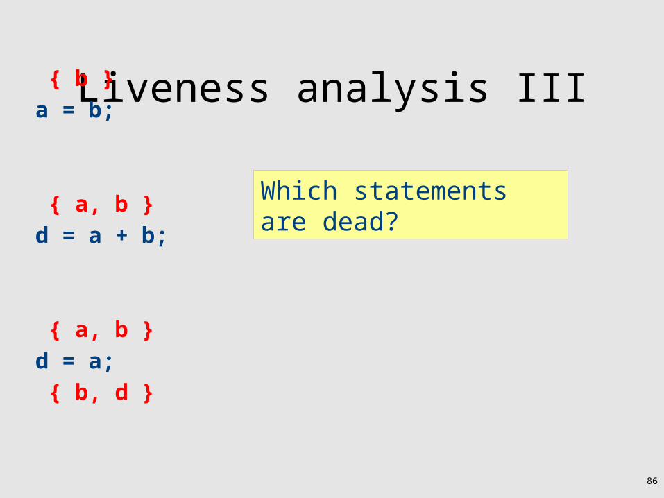
Liveness analysis IIIa = b;
d = a + b;
d = a;
{ b, d }
{ a, b }
{ a, b }
{ b }
Which statements are dead?
86

Dead code eliminationa = b;
d = a + b;
d = a;
{ b, d }
{ a, b }
{ a, b }
{ b }
Which statements are dead?
87

Dead code eliminationa = b;
d = a;
{ b, d }
{ a, b }
{ a, b }
{ b }
88

Dead code eliminationa = b;
d = a;
89
If we further apply copy propagation this statement can be eliminated too
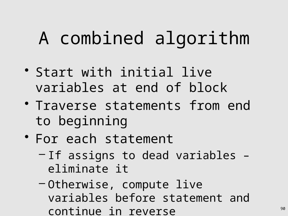
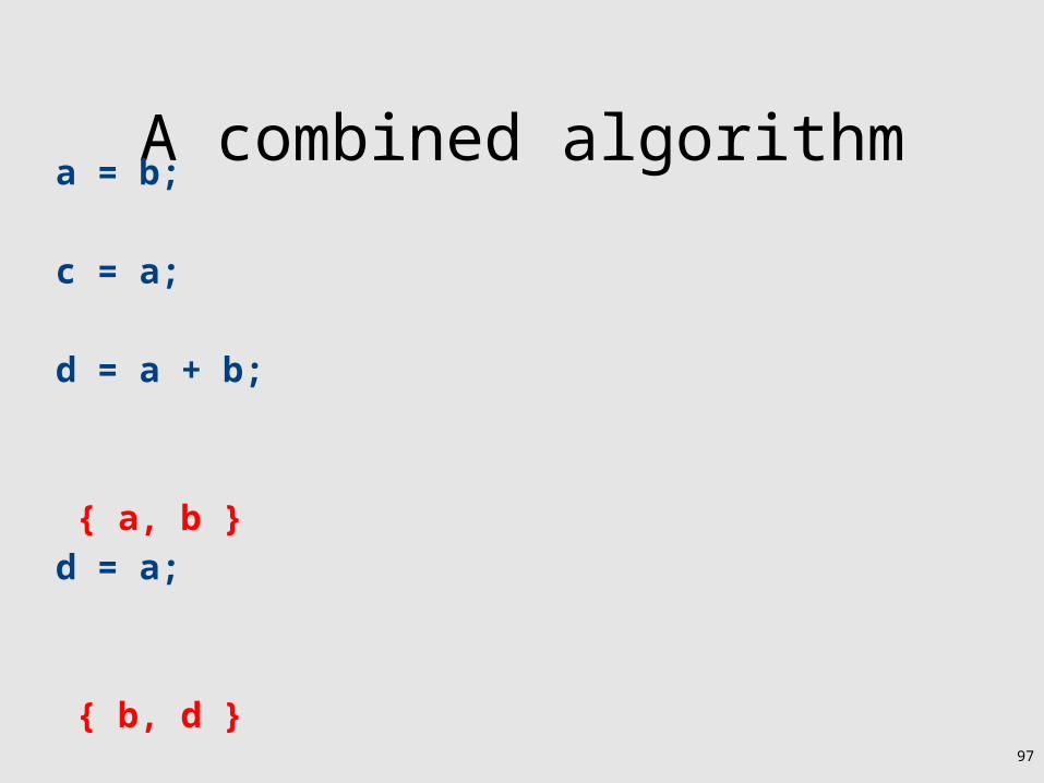
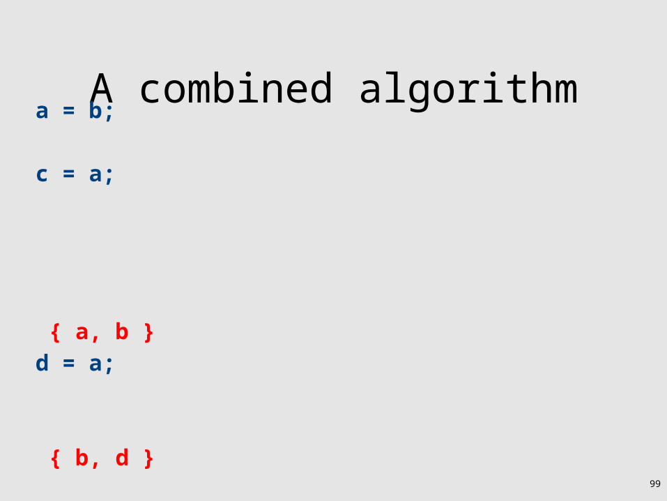
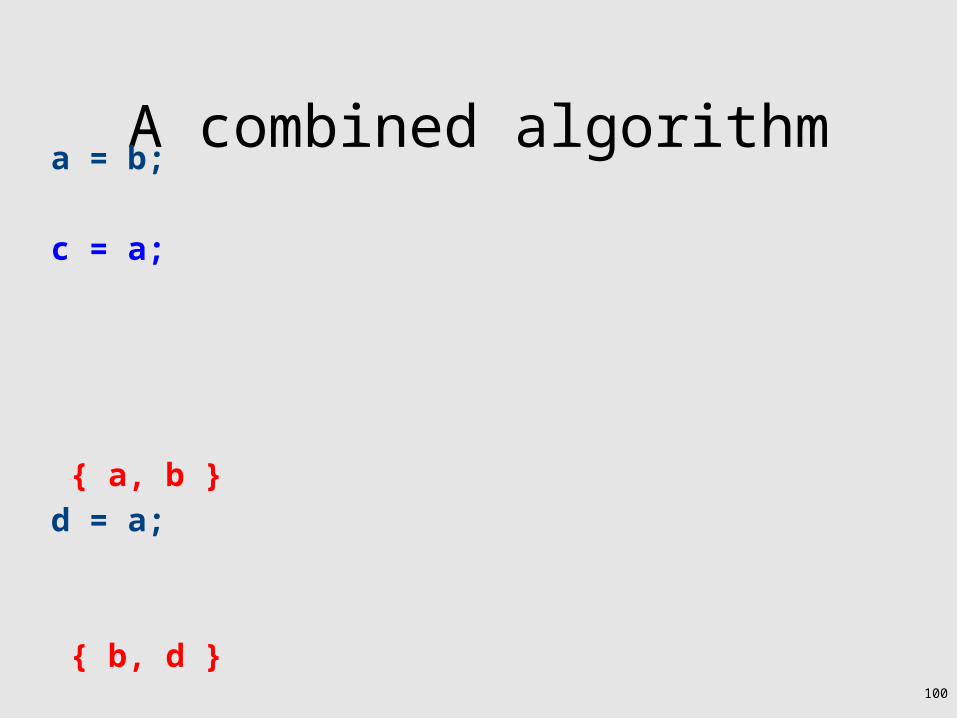
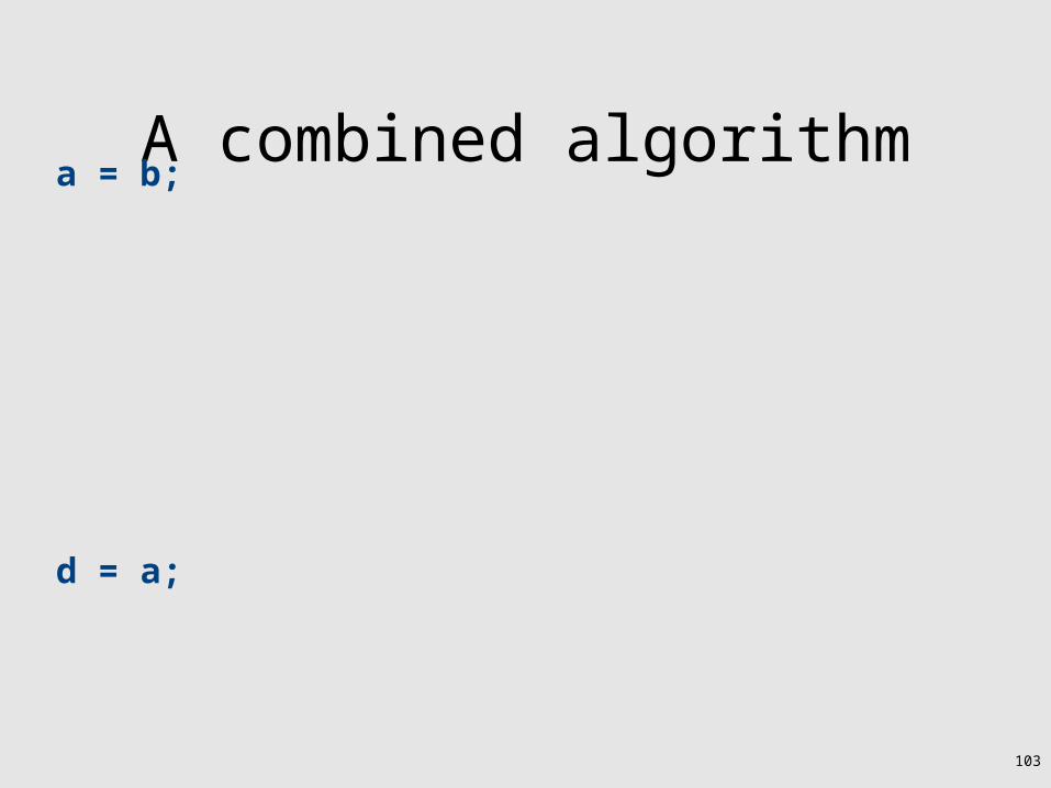
A combined algorithm
• Start with initial live variables at end of block
• Traverse statements from end to beginning• For each statement
– If assigns to dead variables – eliminate it– Otherwise, compute live variables before
statement and continue in reverse
90

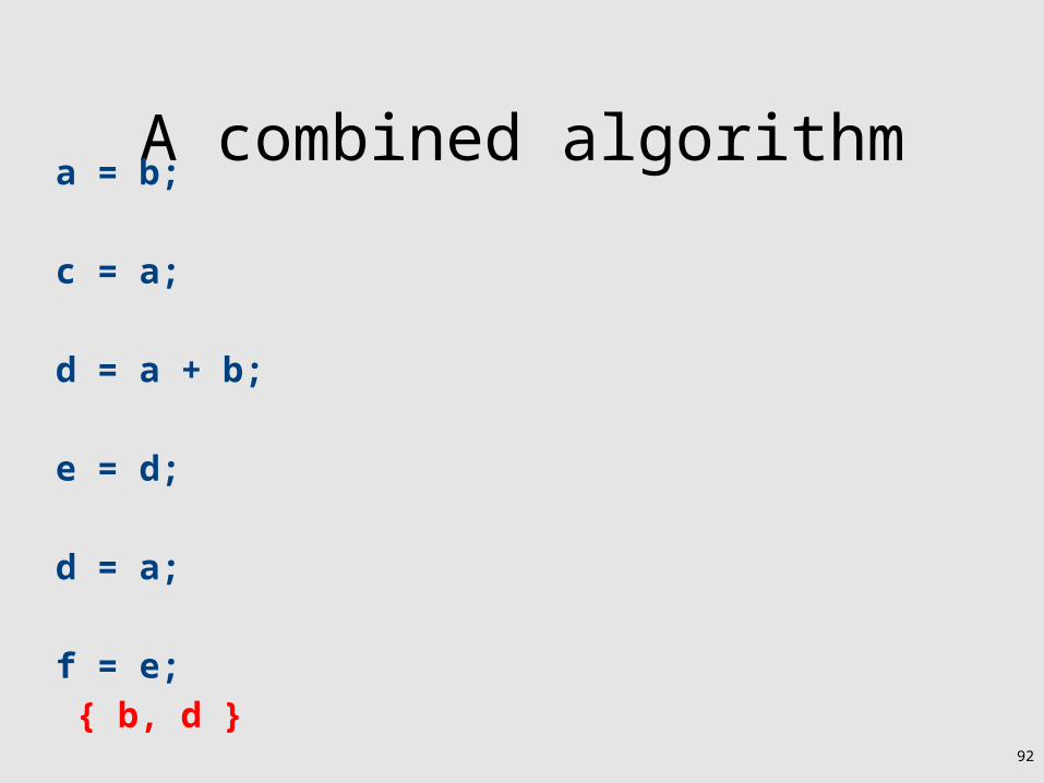
A combined algorithma = b;
c = a;
d = a + b;
e = d;
d = a;
f = e;
91
A combined algorithma = b;
c = a;
d = a + b;
e = d;
d = a;
f = e;
{ b, d }92

A combined algorithma = b;
c = a;
d = a + b;
e = d;
d = a;
f = e;
{ b, d }93
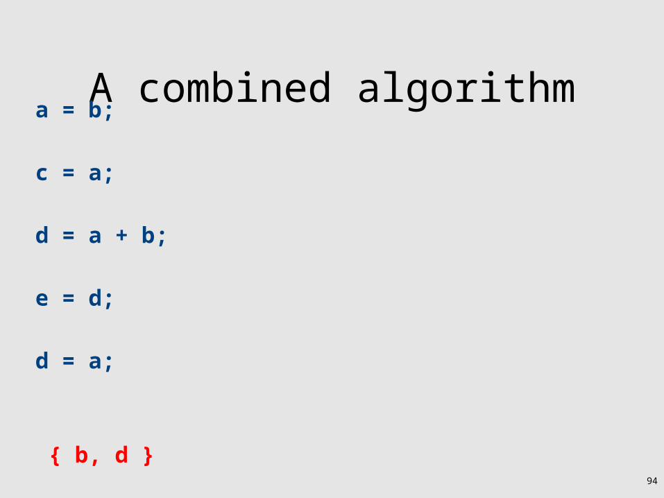
A combined algorithma = b;
c = a;
d = a + b;
e = d;
d = a;
{ b, d }94

A combined algorithma = b;
c = a;
d = a + b;
e = d;
d = a;
{ b, d }
{ a, b }
95

A combined algorithm
96
a = b;
c = a;
d = a + b;
e = d;
d = a;
{ b, d }
{ a, b }
A combined algorithm
97
a = b;
c = a;
d = a + b;
d = a;
{ b, d }
{ a, b }

A combined algorithma = b;
c = a;
d = a + b;
d = a;
{ b, d }
{ a, b }
98
A combined algorithma = b;
c = a;
d = a;
{ b, d }
{ a, b }
99
A combined algorithma = b;
c = a;
d = a;
{ b, d }
{ a, b }
100

A combined algorithma = b;
d = a;
{ b, d }
{ a, b }
101

A combined algorithma = b;
d = a;
{ b, d }
{ a, b }
102
{ b }
A combined algorithma = b;
d = a;
103

104
High-level goals
• Generalize analysis mechanism– Reuse common ingredients for many analyses– Reuse proofs of correctness
• Generalize from basic blocks to entire CFGs– Go from local optimizations to global
optimizations
105
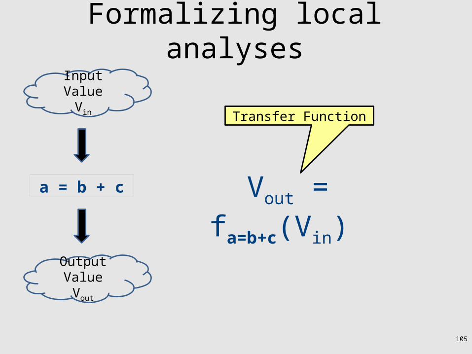
Formalizing local analyses
a = b + c
Output ValueVout
Input ValueVin
Vout = fa=b+c(Vin)
Transfer Function

106
Available Expressions
a = b + c
Output ValueVout
Input ValueVin
Vout = (Vin \ {e | e contains a}) {a=b+c}
Expressions of the forms a=… and x=…a…
107
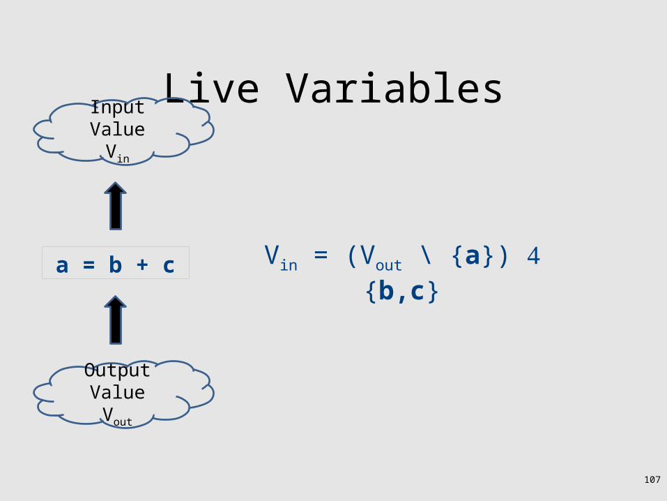
Live Variables
a = b + c
Output ValueVout
Input ValueVin
Vin = (Vout \ {a}) {b,c}

108
Information for a local analysis
• What direction are we going?– Sometimes forward (available expressions)– Sometimes backward (liveness analysis)
• How do we update information after processing a statement?– What are the new semantics?– What information do we know initially?
109
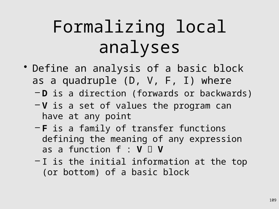
Formalizing local analyses
• Define an analysis of a basic block as a quadruple (D, V, F, I) where– D is a direction (forwards or backwards)– V is a set of values the program can have at any
point– F is a family of transfer functions defining the
meaning of any expression as a function f : V V– I is the initial information at the top (or bottom)
of a basic block

110
Available Expressions
• Direction: Forward• Values: Sets of expressions assigned to variables• Transfer functions: Given a set of variable
assignments V and statement a = b + c:– Remove from V any expression containing a as a
subexpression– Add to V the expression a = b + c– Formally: Vout = (Vin \ {e | e contains a}) {a = b + c}
• Initial value: Empty set of expressions

111
Liveness Analysis
• Direction: Backward• Values: Sets of variables• Transfer functions: Given a set of variable assignments V
and statement a = b + c:• Remove a from V (any previous value of a is now dead.)• Add b and c to V (any previous value of b or c is now live.)• Formally: Vin = (Vout \ {a}) {b,c}• Initial value: Depends on semantics of language
– E.g., function arguments and return values (pushes)– Result of local analysis of other blocks as part of a
global analysis
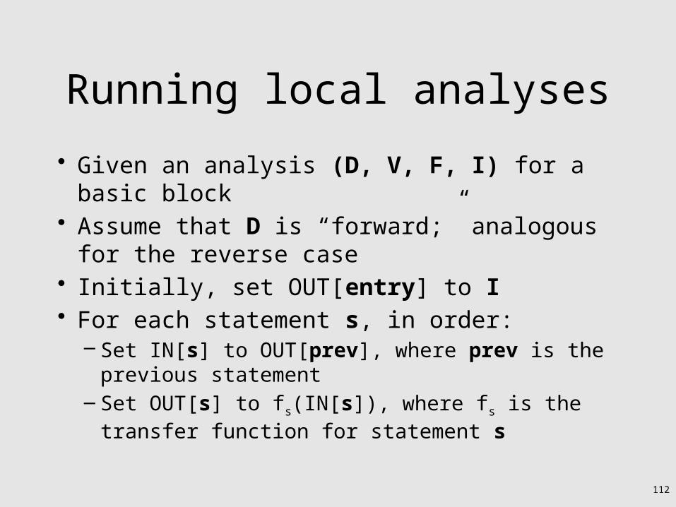
Running local analyses
• Given an analysis (D, V, F, I) for a basic block• Assume that D is “forward;” analogous for the
reverse case• Initially, set OUT[entry] to I• For each statement s, in order:
– Set IN[s] to OUT[prev], where prev is the previous statement
– Set OUT[s] to fs(IN[s]), where fs is the transfer function for statement s
112

Global Optimizations
113

114
Global analysis
• A global analysis is an analysis that works on a control-flow graph as a whole
• Substantially more powerful than a local analysis– (Why?)
• Substantially more complicated than a local analysis– (Why?)
115
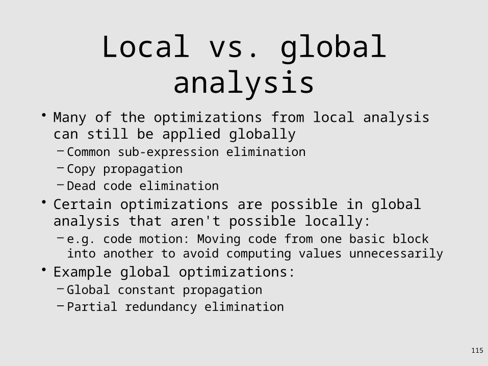
Local vs. global analysis
• Many of the optimizations from local analysis can still be applied globally– Common sub-expression elimination– Copy propagation– Dead code elimination
• Certain optimizations are possible in global analysis that aren't possible locally:– e.g. code motion: Moving code from one basic block into another to
avoid computing values unnecessarily• Example global optimizations:
– Global constant propagation– Partial redundancy elimination
116
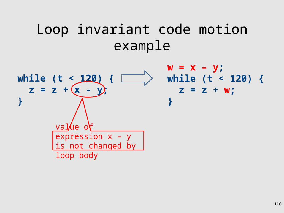
Loop invariant code motion example
while (t < 120) { z = z + x - y;}
w = x – y;while (t < 120) { z = z + w;}
value of expression x – y is not changed by loop body
117
Why global analysis is hard
• Need to be able to handle multiple predecessors/successors for a basic block
• Need to be able to handle multiple paths through the control-flow graph, and may need to iterate multiple times to compute the final value (but the analysis still needs to terminate!)
• Need to be able to assign each basic block a reasonable default value for before we've analyzed it

118
Global dead code elimination
• Local dead code elimination needed to know what variables were live on exit from a basic block
• This information can only be computed as part of a global analysis
• How do we modify our liveness analysis to handle a CFG?

119
CFGs without loops
Exit
x = a + b;y = c + d;
y = a + b;x = c + d;a = b + c;
b = c + d;e = c + d;Entry

120
CFGs without loops
Exit
x = a + b;y = c + d;
y = a + b;x = c + d;a = b + c;
b = c + d;e = c + d;Entry
{x, y}
{x, y}
{a, b, c, d}
{a, b, c, d} {a, b, c, d}
{a, b, c, d}{b, c, d}
{a, b, c, d}
{a, c, d}
?
Which variables may be live on some execution path?

121
CFGs without loops
Exit
x = a + b;y = c + d;
y = a + b;x = c + d;a = b + c;
b = c + d;e = c + d;Entry
{x, y}
{x, y}
{a, b, c, d}
{a, b, c, d} {a, b, c, d}
{a, b, c, d}{b, c, d}
{a, b, c, d}
{a, c, d}

122
CFGs without loops
Exit
x = a + b;y = c + d;
a = b + c;
b = c + d;Entry

123
CFGs without loops
Exit
x = a + b;y = c + d;
a = b + c;
b = c + d;Entry

124
Major changes – part 1
• In a local analysis, each statement has exactly one predecessor
• In a global analysis, each statement may have multiple predecessors
• A global analysis must have some means of combining information from all predecessors of a basic block

125
CFGs without loops
Exit
x = a + b;y = c + d;
y = a + b;x = c + d;a = b + c;
b = c + d;e = c + d;Entry
{x, y}
{x, y}
{a, b, c, d}
{a, b, c, d} {a, b, c, d}
{a, b, c, d}{b, c, d}
{b, c, d}
{c, d} Need to combine currently-computed value with new value
Need to combine currently-computed value with new value

126
CFGs without loops
Exit
x = a + b;y = c + d;
y = a + b;x = c + d;a = b + c;
b = c + d;e = c + d;Entry
{x, y}
{x, y}
{a, b, c, d}
{a, b, c, d} {a, b, c, d}
{a, b, c, d}{b, c, d}
{a, b, c, d}
{c, d}

127
CFGs without loops
Exit
x = a + b;y = c + d;
y = a + b;x = c + d;a = b + c;
b = c + d;e = c + d;Entry
{x, y}
{x, y}
{a, b, c, d}
{a, b, c, d} {a, b, c, d}
{a, b, c, d}{b, c, d}
{a, b, c, d}
{a, c, d}

128
Major changes – part 2
• In a local analysis, there is only one possible path through a basic block
• In a global analysis, there may be many paths through a CFG
• May need to recompute values multiple times as more information becomes available
• Need to be careful when doing this not to loop infinitely!– (More on that later)
129
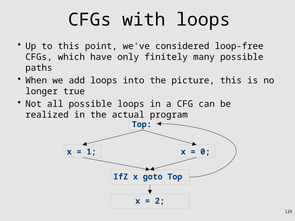
CFGs with loops• Up to this point, we've considered loop-free CFGs,
which have only finitely many possible paths• When we add loops into the picture, this is no longer
true• Not all possible loops in a CFG can be realized in the
actual program
IfZ x goto Top
x = 1;
Top:
x = 0;
x = 2;

130
CFGs with loops• Up to this point, we've considered loop-free CFGs, which
have only finitely many possible paths• When we add loops into the picture, this is no longer true• Not all possible loops in a CFG can be realized in the actual
program• Sound approximation: Assume that every possible path
through the CFG corresponds to a valid execution– Includes all realizable paths, but some additional paths as well– May make our analysis less precise (but still sound)– Makes the analysis feasible; we'll see how later

131
CFGs with loops
Exit
a = a + b;d = b + c;
c = a + b;a = b + c;d = a + c;
b = c + d;c = c + d;IfZ ...
Entry
{a}
?

132
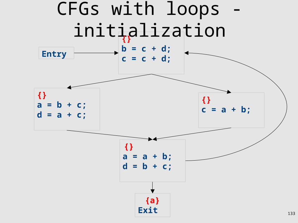
Major changes – part 3
• In a local analysis, there is always a well defined “first” statement to begin processing
• In a global analysis with loops, every basic block might depend on every other basic block
• To fix this, we need to assign initial values to all of the blocks in the CFG
133
CFGs with loops - initialization
Exit
a = a + b;d = b + c;
c = a + b;a = b + c;d = a + c;
b = c + d;c = c + d;Entry
{a}
{}{}
{}
{}

134
CFGs with loops - iteration
Exit
a = a + b;d = b + c;
c = a + b;a = b + c;d = a + c;
b = c + d;c = c + d;Entry
{a}
{}{}
{}
{}
{a}

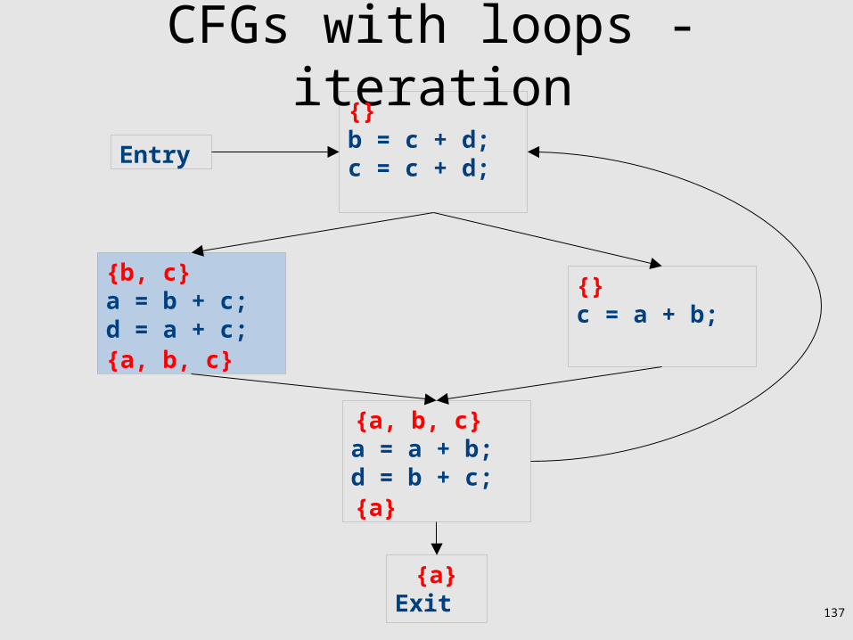
135
CFGs with loops - iteration
Exit
a = a + b;d = b + c;
c = a + b;a = b + c;d = a + c;
b = c + d;c = c + d;Entry
{a}
{}{}
{}
{a, b, c}
{a}

136
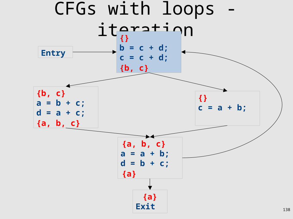
CFGs with loops - iteration
Exit
a = a + b;d = b + c;
c = a + b;a = b + c;d = a + c;
b = c + d;c = c + d;Entry
{a}
{}{}
{}
{a, b, c}
{a}
{a, b, c}
137
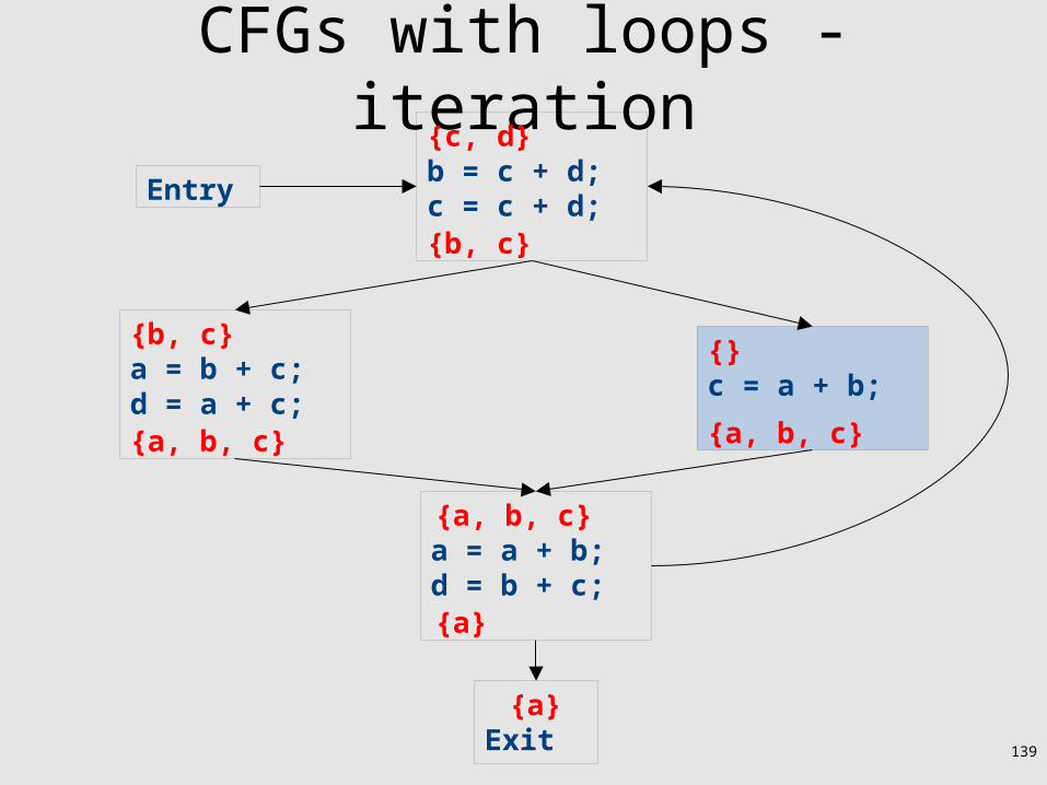
CFGs with loops - iteration
Exit
a = a + b;d = b + c;
c = a + b;a = b + c;d = a + c;
b = c + d;c = c + d;Entry
{a}
{}{b, c}
{}
{a, b, c}
{a}
{a, b, c}
138
CFGs with loops - iteration
Exit
a = a + b;d = b + c;
c = a + b;a = b + c;d = a + c;
b = c + d;c = c + d;Entry
{a}
{}{b, c}
{}
{a, b, c}
{a}
{a, b, c}
{b, c}
139
CFGs with loops - iteration
Exit
a = a + b;d = b + c;
c = a + b;a = b + c;d = a + c;
b = c + d;c = c + d;Entry
{a}
{}{b, c}
{c, d}
{a, b, c}
{a}
{a, b, c}
{b, c}
{a, b, c}

140
CFGs with loops - iteration
Exit
a = a + b;d = b + c;
c = a + b;a = b + c;d = a + c;
b = c + d;c = c + d;Entry
{a}
{a, b}{b, c}
{c, d}
{a, b, c}
{a}
{a, b, c}
{b, c}
{a, b, c}

141
CFGs with loops - iteration
Exit
a = a + b;d = b + c;
c = a + b;a = b + c;d = a + c;
b = c + d;c = c + d;Entry
{a}
{a, b}{b, c}
{c, d}
{a, b, c}
{a}
{a, b, c}
{b, c}
{a, b, c}
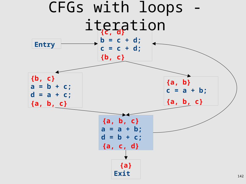
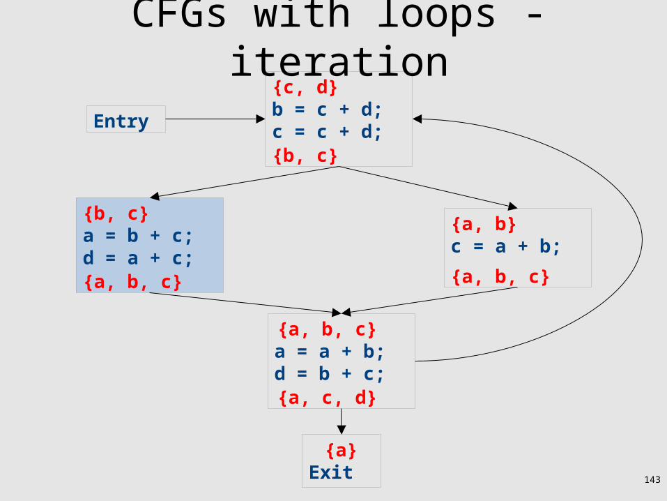
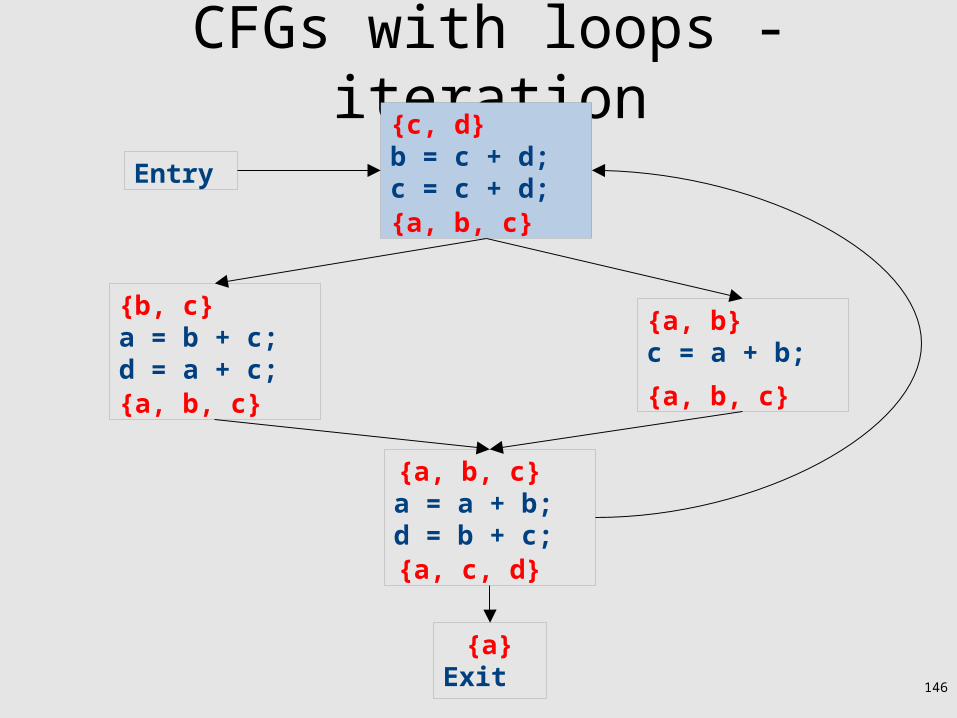
142
CFGs with loops - iteration
Exit
a = a + b;d = b + c;
c = a + b;a = b + c;d = a + c;
b = c + d;c = c + d;Entry
{a}
{a, b}{b, c}
{c, d}
{a, b, c}
{a, c, d}
{a, b, c}
{b, c}
{a, b, c}
143
CFGs with loops - iteration
Exit
a = a + b;d = b + c;
c = a + b;a = b + c;d = a + c;
b = c + d;c = c + d;Entry
{a}
{a, b}{b, c}
{c, d}
{a, b, c}
{a, c, d}
{a, b, c}
{b, c}
{a, b, c}

144
CFGs with loops - iteration
Exit
a = a + b;d = b + c;
c = a + b;a = b + c;d = a + c;
b = c + d;c = c + d;Entry
{a}
{a, b}{b, c}
{c, d}
{a, b, c}
{a, c, d}
{a, b, c}
{b, c}
{a, b, c}

145
CFGs with loops - iteration
Exit
a = a + b;d = b + c;
c = a + b;a = b + c;d = a + c;
b = c + d;c = c + d;Entry
{a}
{a, b}{b, c}
{c, d}
{a, b, c}
{a, c, d}
{a, b, c}
{b, c}
{a, b, c}
146
CFGs with loops - iteration
Exit
a = a + b;d = b + c;
c = a + b;a = b + c;d = a + c;
b = c + d;c = c + d;Entry
{a}
{a, b}{b, c}
{c, d}
{a, b, c}
{a, c, d}
{a, b, c}
{a, b, c}
{a, b, c}

147
CFGs with loops - iteration
Exit
a = a + b;d = b + c;
c = a + b;a = b + c;d = a + c;
b = c + d;c = c + d;Entry
{a}
{a, b}{b, c}
{a, c, d}
{a, b, c}
{a, c, d}
{a, b, c}
{a, b, c}
{a, b, c}

148
CFGs with loops - iteration
Exit
a = a + b;d = b + c;
c = a + b;a = b + c;d = a + c;
b = c + d;c = c + d;Entry
{a}
{a, b}{b, c}
{a, c, d}
{a, b, c}
{a, c, d}
{a, b, c}
{a, b, c}
{a, b, c}
149
Summary of differences
• Need to be able to handle multiple predecessors/successors for a basic block
• Need to be able to handle multiple paths through the control-flow graph, and may need to iterate multiple times to compute the final value– But the analysis still needs to terminate!
• Need to be able to assign each basic block a reasonable default value for before we've analyzed it

150
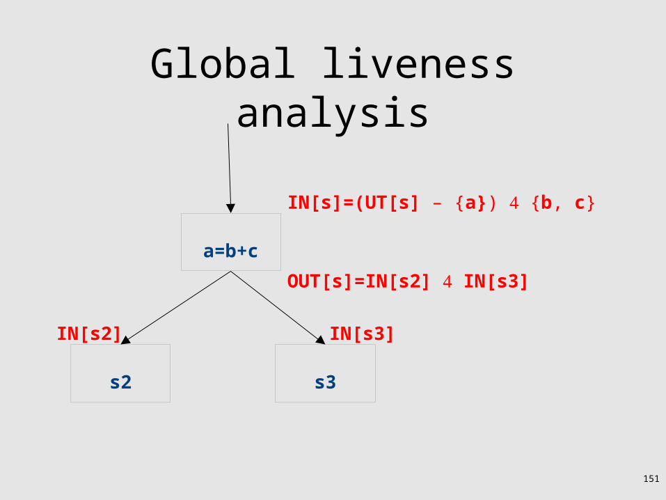
Global liveness analysis• Initially, set IN[s] = { } for each statement s• Set IN[exit] to the set of variables known to be
live on exit (language-specific knowledge)• Repeat until no changes occur:
– For each statement s of the form a = b + c, in any order you'd like:• Set OUT[s] to set union of IN[p] for each successor p of s• Set IN[s] to (OUT[s] – a) {b, c}.
• Yet another fixed-point iteration!
151
Global liveness analysis
a=b+c
s2 s3
IN[s2] IN[s3]
OUT[s]=IN[s2] IN[s3]
IN[s]=(UT[s] – {a}) {b, c}

152
Why does this work?• To show correctness, we need to show that
– The algorithm eventually terminates, and– When it terminates, it has a sound answer
• Termination argument:– Once a variable is discovered to be live during some point of the analysis,
it always stays live– Only finitely many variables and finitely many places where a variable
can become live• Soundness argument (sketch):
– Each individual rule, applied to some set, correctly updates liveness in that set
– When computing the union of the set of live variables, a variable is only live if it was live on some path leaving the statement

153
Abstract Interpretation
• Theoretical foundations of program analysis
• Cousot and Cousot 1977
• Abstract meaning of programs– Executed at compile time

154
Another view of local optimization
• In local optimization, we want to reason about some property of the runtime behavior of the program
• Could we run the program and just watch what happens?
• Idea: Redefine the semantics of our programming language to give us information about our analysis
155
Properties of local analysis
• The only way to find out what a program will actually do is to run it
• Problems:– The program might not terminate– The program might have some behavior we didn't see
when we ran it on a particular input• However, this is not a problem inside a basic block
– Basic blocks contain no loops– There is only one path through the basic block
156
Assigning new semantics
• Example: Available Expressions• Redefine the statement a = b + c to mean
“a now holds the value of b + c, and any variable holding the value a is now invalid”
• Run the program assuming these new semantics
• Treat the optimizer as an interpreter for these new semantics
157
Theory to the rescue
• Building up all of the machinery to design this analysis was tricky
• The key ideas, however, are mostly independent of the analysis:– We need to be able to compute functions describing the
behavior of each statement– We need to be able to merge several subcomputations
together– We need an initial value for all of the basic blocks
• There is a beautiful formalism that captures many of these properties

158
Join semilattices
• A join semilattice is a ordering defined on a set of elements• Any two elements have some join that is the smallest
element larger than both elements• There is a unique bottom element, which is smaller than all
other elements• Intuitively:
– The join of two elements represents combining information from two elements by an overapproximation
• The bottom element represents “no information yet” or “the least conservative possible answer”

159
Join semilattice for liveness
{}
{a} {b} {c}
{a, b} {a, c} {b, c}
{a, b, c}
Bottom element

160
What is the join of {b} and {c}?
{}
{a} {b} {c}
{a, b} {a, c} {b, c}
{a, b, c}

161
What is the join of {b} and {c}?
{}
{a} {b} {c}
{a, b} {a, c} {b, c}
{a, b, c}

162
What is the join of {b} and {a,c}?
{}
{a} {b} {c}
{a, b} {a, c} {b, c}
{a, b, c}

163
What is the join of {b} and {a,c}?
{}
{a} {b} {c}
{a, b} {a, c} {b, c}
{a, b, c}
164
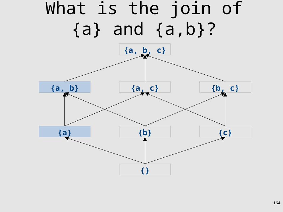
What is the join of {a} and {a,b}?
{}
{a} {b} {c}
{a, b} {a, c} {b, c}
{a, b, c}

165
What is the join of {a} and {a,b}?
{}
{a} {b} {c}
{a, b} {a, c} {b, c}
{a, b, c}
166
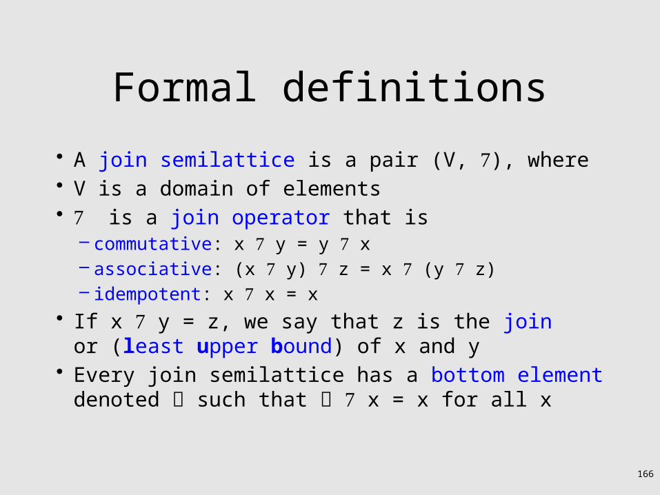
Formal definitions
• A join semilattice is a pair (V, ), where• V is a domain of elements• is a join operator that is
– commutative: x y = y x– associative: (x y) z = x (y z)– idempotent: x x = x
• If x y = z, we say that z is the joinor (least upper bound) of x and y
• Every join semilattice has a bottom element denoted such that x = x for all x

167
Join semilattices and ordering
{}
{a} {b} {c}
{a, b} {a, c} {b, c}
{a, b, c}Greater
Lower
168
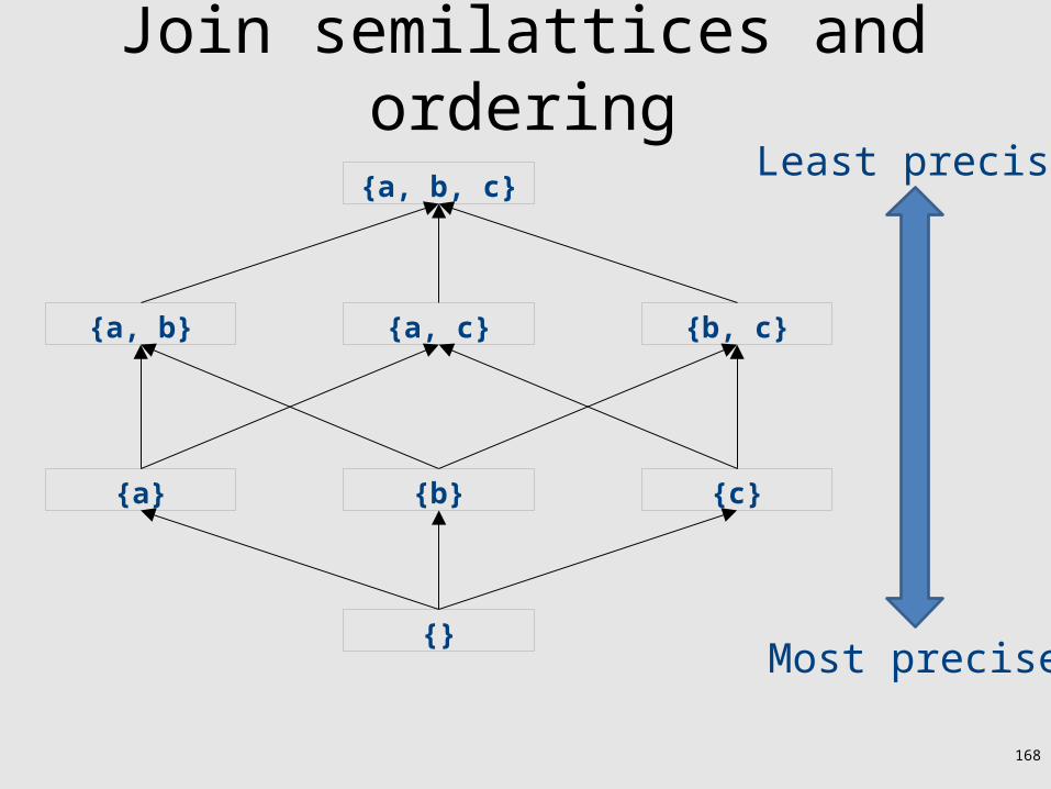
Join semilattices and ordering
{}
{a} {b} {c}
{a, b} {a, c} {b, c}
{a, b, c}Least precise
Most precise

169
Join semilattices and orderings
• Every join semilattice (V, ) induces an ordering relationship over its elements
• Define x y iff x y = y• Need to prove
– Reflexivity: x x– Antisymmetry: If x y and y x, then x = y– Transitivity: If x y and y z, then x z

170
An example join semilattice
• The set of natural numbers and the max function• Idempotent
– max{a, a} = a• Commutative
– max{a, b} = max{b, a}• Associative
– max{a, max{b, c}} = max{max{a, b}, c}• Bottom element is 0:
– max{0, a} = a• What is the ordering over these elements?

171
A join semilattice for liveness
• Sets of live variables and the set union operation• Idempotent:
– x x = x• Commutative:
– x y = y x• Associative:
– (x y) z = x (y z)• Bottom element:
– The empty set: Ø x = x• What is the ordering over these elements?

172
Semilattices and program analysis
• Semilattices naturally solve many of the problems we encounter in global analysis
• How do we combine information from multiple basic blocks?
• What value do we give to basic blocks we haven't seen yet?
• How do we know that the algorithm always terminates?

173
Semilattices and program analysis
• Semilattices naturally solve many of the problems we encounter in global analysis
• How do we combine information from multiple basic blocks?– Take the join of all information from those blocks
• What value do we give to basic blocks we haven't seen yet?– Use the bottom element
• How do we know that the algorithm always terminates?– Actually, we still don't! More on that later
174
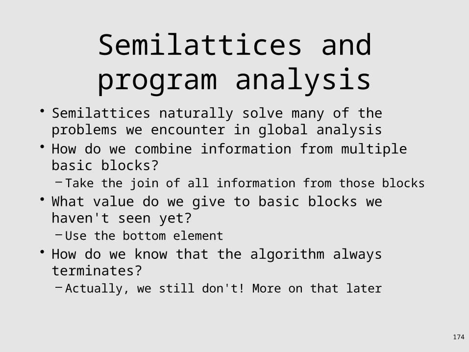
Semilattices and program analysis
• Semilattices naturally solve many of the problems we encounter in global analysis
• How do we combine information from multiple basic blocks?– Take the join of all information from those blocks
• What value do we give to basic blocks we haven't seen yet?– Use the bottom element
• How do we know that the algorithm always terminates?– Actually, we still don't! More on that later

175
A general framework
• A global analysis is a tuple (D, V, , F, I), where– D is a direction (forward or backward)
• The order to visit statements within a basic block, not the order in which to visit the basic blocks
– V is a set of values– is a join operator over those values– F is a set of transfer functions f : V V– I is an initial value
• The only difference from local analysis is the introduction of the join operator

176
Running global analyses
• Assume that (D, V, , F, I) is a forward analysis• Set OUT[s] = for all statements s• Set OUT[entry] = I• Repeat until no values change:
– For each statement s with predecessorsp1, p2, … , pn:• Set IN[s] = OUT[p1] OUT[p2] … OUT[pn]• Set OUT[s] = fs (IN[s])
• The order of this iteration does not matter– This is sometimes called chaotic iteration

177
For comparison
• Set OUT[s] = for all statements s
• Set OUT[entry] = I• Repeat until no values
change:– For each statement s with
predecessorsp1, p2, … , pn:
• Set IN[s] = OUT[p1] OUT[p2] … OUT[pn]
• Set OUT[s] = fs (IN[s])
• Set IN[s] = {} for all statements s
• Set OUT[exit] = the set of variables known to be live on exit
• Repeat until no values change:– For each statement s of the
form a=b+c:• Set OUT[s] = set union of IN[x]
for each successor x of s• Set IN[s] = (OUT[s]-{a}) {b,c}

178
The dataflow framework
• This form of analysis is called the dataflow framework
• Can be used to easily prove an analysis is sound
• With certain restrictions, can be used to prove that an analysis eventually terminates– Again, more on that later

179
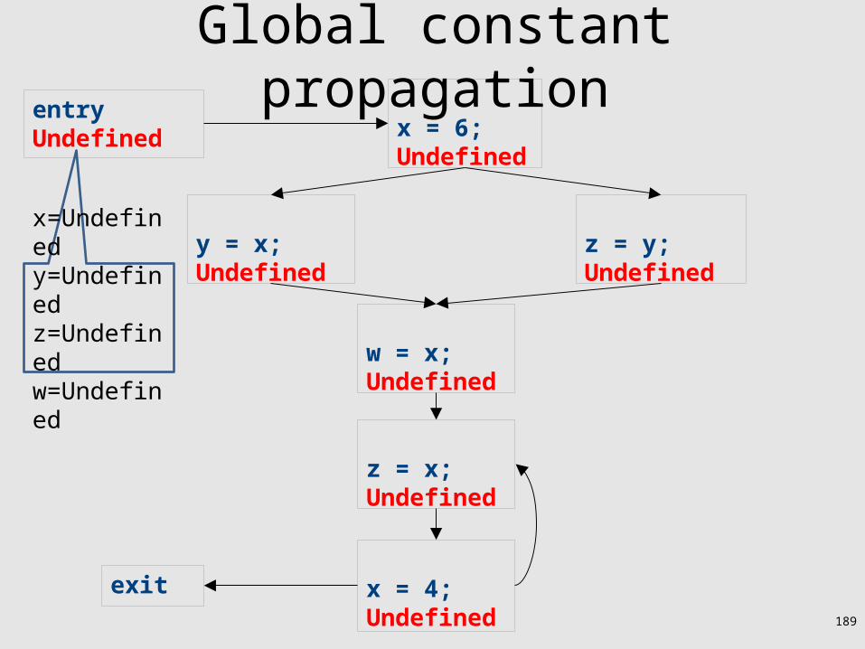
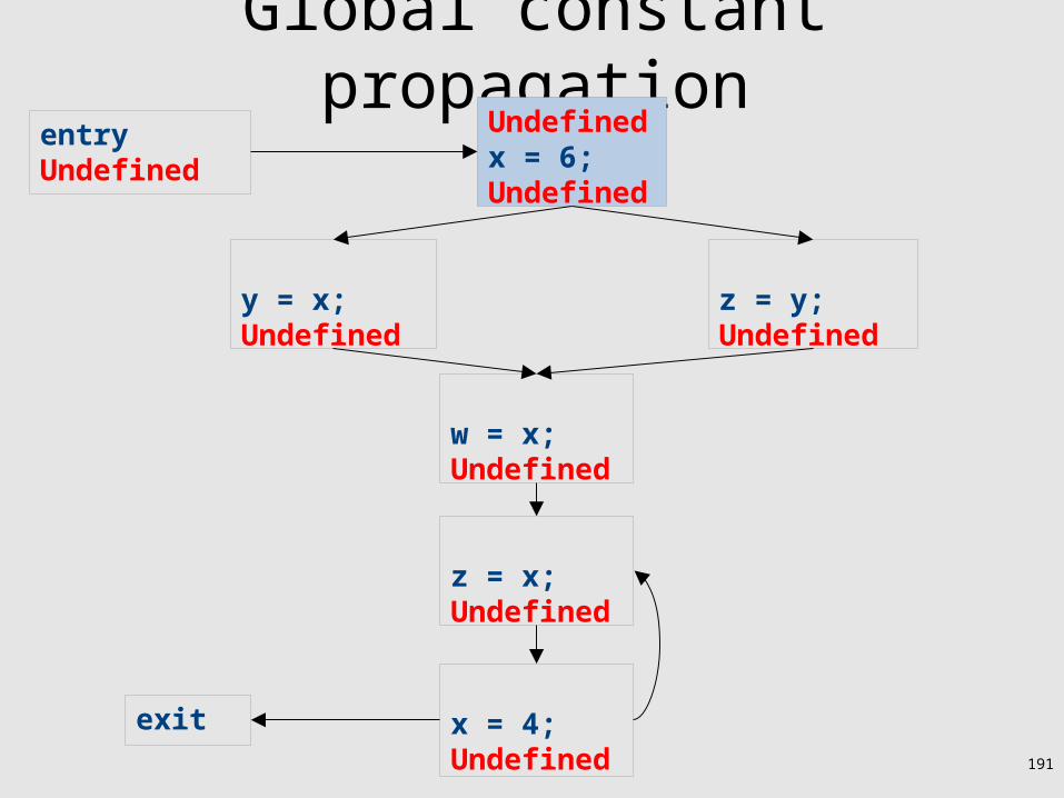
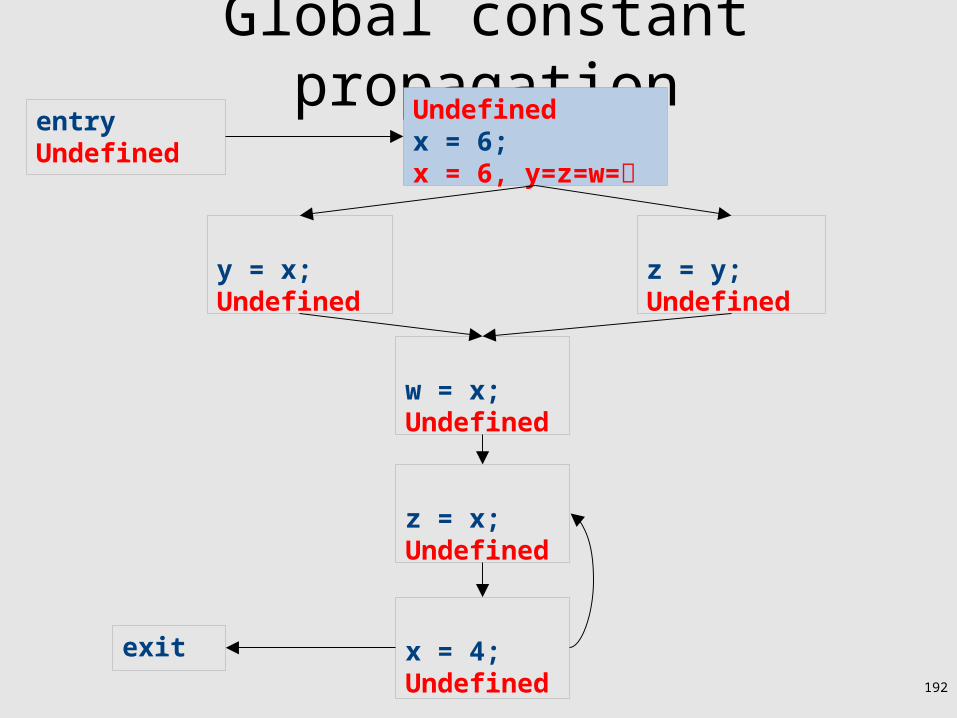
Global constant propagation
• Constant propagation is an optimization that replaces each variable that is known to be a constant value with that constant
• An elegant example of the dataflow framework

180
Global constant propagation
exit x = 4;
z = x;
w = x;
y = x; z = y;
x = 6;entry

181
Global constant propagation
exit x = 4;
z = x;
w = x;
y = x; z = y;
x = 6;entry

182
Global constant propagation
exit x = 4;
z = x;
w = 6;
y = 6; z = y;
x = 6;entry
183
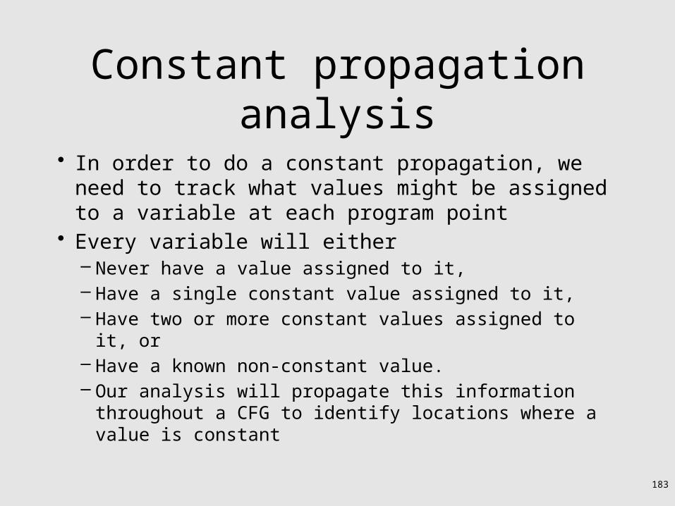
Constant propagation analysis
• In order to do a constant propagation, we need to track what values might be assigned to a variable at each program point
• Every variable will either– Never have a value assigned to it,– Have a single constant value assigned to it,– Have two or more constant values assigned to it, or– Have a known non-constant value.– Our analysis will propagate this information throughout a
CFG to identify locations where a value is constant
184
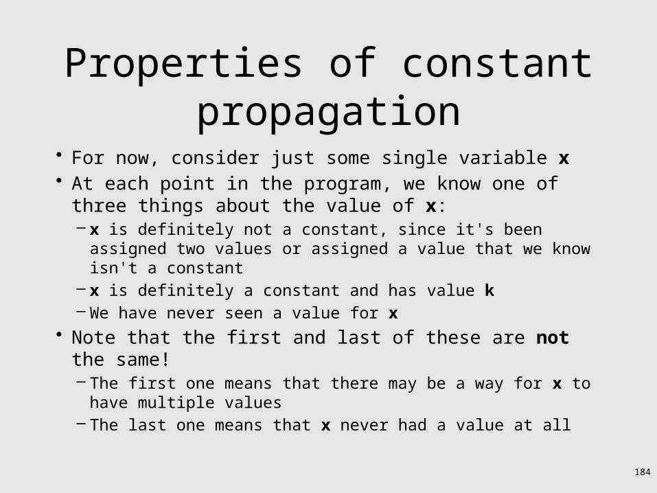
Properties of constant propagation
• For now, consider just some single variable x• At each point in the program, we know one of three things
about the value of x:– x is definitely not a constant, since it's been assigned two values
or assigned a value that we know isn't a constant– x is definitely a constant and has value k– We have never seen a value for x
• Note that the first and last of these are not the same!– The first one means that there may be a way for x to have
multiple values– The last one means that x never had a value at all
185
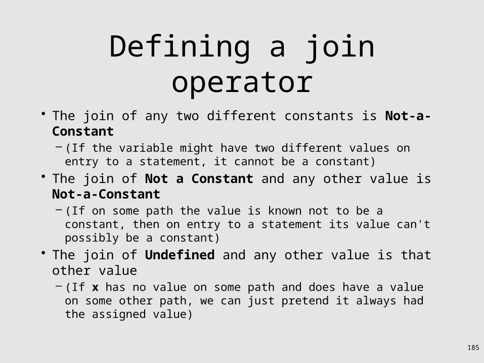
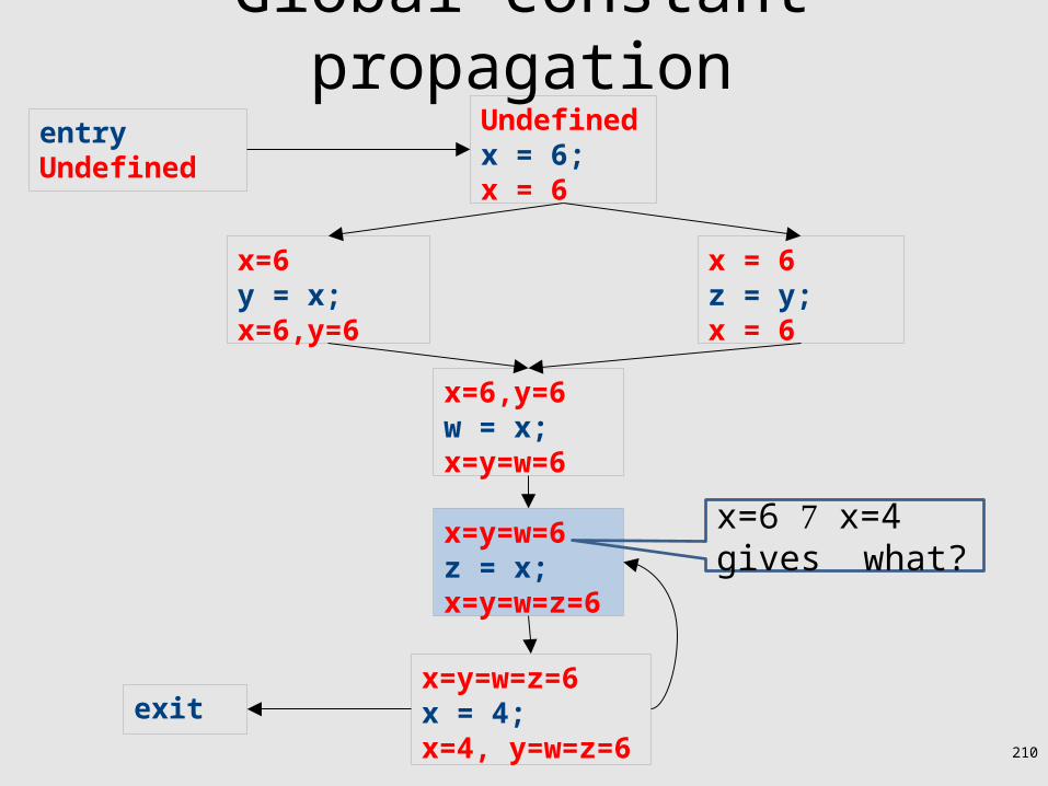
Defining a join operator
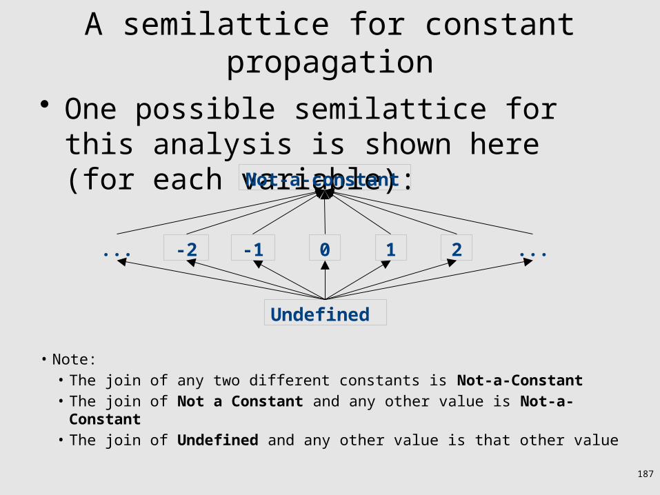
• The join of any two different constants is Not-a-Constant– (If the variable might have two different values on entry to a
statement, it cannot be a constant)• The join of Not a Constant and any other value is Not-a-
Constant– (If on some path the value is known not to be a constant, then on
entry to a statement its value can't possibly be a constant)• The join of Undefined and any other value is that other
value– (If x has no value on some path and does have a value on some
other path, we can just pretend it always had the assigned value)
186
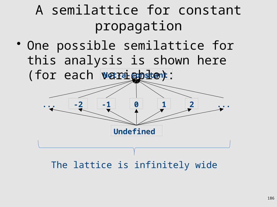
A semilattice for constant propagation• One possible semilattice for this analysis is
shown here (for each variable):
Undefined
0-1-2 1 2 ......
Not-a-constant
The lattice is infinitely wide
187
A semilattice for constant propagation• One possible semilattice for this analysis is
shown here (for each variable):
Undefined
0-1-2 1 2 ......
Not-a-constant
• Note:• The join of any two different constants is Not-a-Constant• The join of Not a Constant and any other value is Not-a-Constant• The join of Undefined and any other value is that other value

188
Global constant propagation
exit x = 4;Undefined
z = x;Undefined
w = x;
y = x; z = y;
x = 6;entry
189
Global constant propagation
exit x = 4;Undefined
z = x;Undefined
w = x;Undefined
y = x;Undefined
z = y;Undefined
x = 6;Undefined
entryUndefined
x=Undefinedy=Undefinedz=Undefinedw=Undefined

190
Global constant propagation
exit x = 4;Undefined
z = x;Undefined
w = x;Undefined
y = x;Undefined
z = y;Undefined
x = 6;Undefined
entryUndefined
191
Global constant propagation
exit x = 4;Undefined
z = x;Undefined
w = x;Undefined
y = x;Undefined
z = y;Undefined
Undefinedx = 6;Undefined
entryUndefined
192
Global constant propagation
exit x = 4;Undefined
z = x;Undefined
w = x;Undefined
y = x;Undefined
z = y;Undefined
Undefinedx = 6;x = 6, y=z=w=
entryUndefined

193
Global constant propagation
exit x = 4;Undefined
z = x;Undefined
w = x;Undefined
y = x;Undefined
z = y;Undefined
Undefinedx = 6;x = 6, y=z=w=
entryUndefined

194
Global constant propagation
exit x = 4;Undefined
z = x;Undefined
w = x;Undefined
x=6y = x;Undefined
z = y;Undefined
Undefinedx = 6;x = 6
entryUndefined

195
Global constant propagation
exit x = 4;Undefined
z = x;Undefined
w = x;Undefined
x=6y = x;x=6,y=6
z = y;Undefined
Undefinedx = 6;x = 6
entryUndefined

196
Global constant propagation
exit x = 4;Undefined
z = x;Undefined
w = x;Undefined
x=6y = x;x=6,y=6
z = y;Undefined
Undefinedx = 6;x = 6
entryUndefined
y=6 y=Undefined gives what?
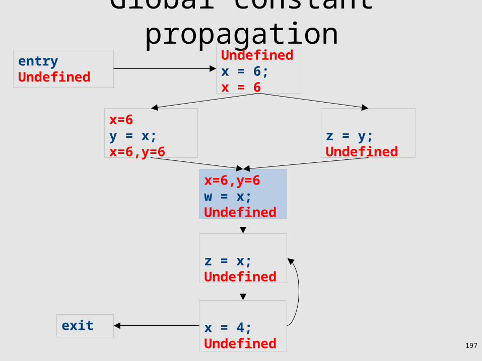
197
Global constant propagation
exit x = 4;Undefined
z = x;Undefined
x=6,y=6w = x;Undefined
x=6y = x;x=6,y=6
z = y;Undefined
Undefinedx = 6;x = 6
entryUndefined

198
Global constant propagation
exit x = 4;Undefined
z = x;Undefined
x=6,y=6w = x;Undefined
x=6y = x;x=6,y=6
z = y;Undefined
Undefinedx = 6;x = 6
entryUndefined
199
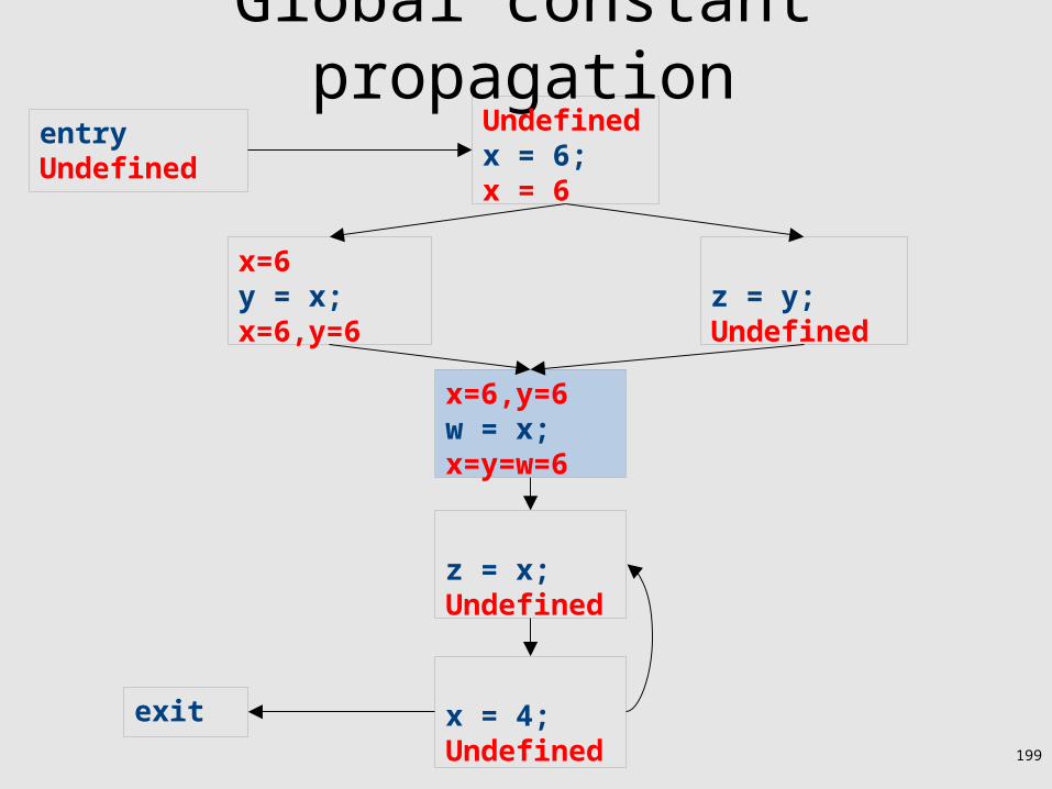
Global constant propagation
exit x = 4;Undefined
z = x;Undefined
x=6,y=6w = x;x=y=w=6
x=6y = x;x=6,y=6
z = y;Undefined
Undefinedx = 6;x = 6
entryUndefined

200
Global constant propagation
exit x = 4;Undefined
z = x;Undefined
x=6,y=6w = x;x=y=w=6
x=6y = x;x=6,y=6
z = y;Undefined
Undefinedx = 6;x = 6
entryUndefined

201
Global constant propagation
exit x = 4;Undefined
x=y=w=6z = x;Undefined
x=6,y=6w = x;x=y=w=6
x=6y = x;x=6,y=6
z = y;Undefined
Undefinedx = 6;x = 6
entryUndefined
202
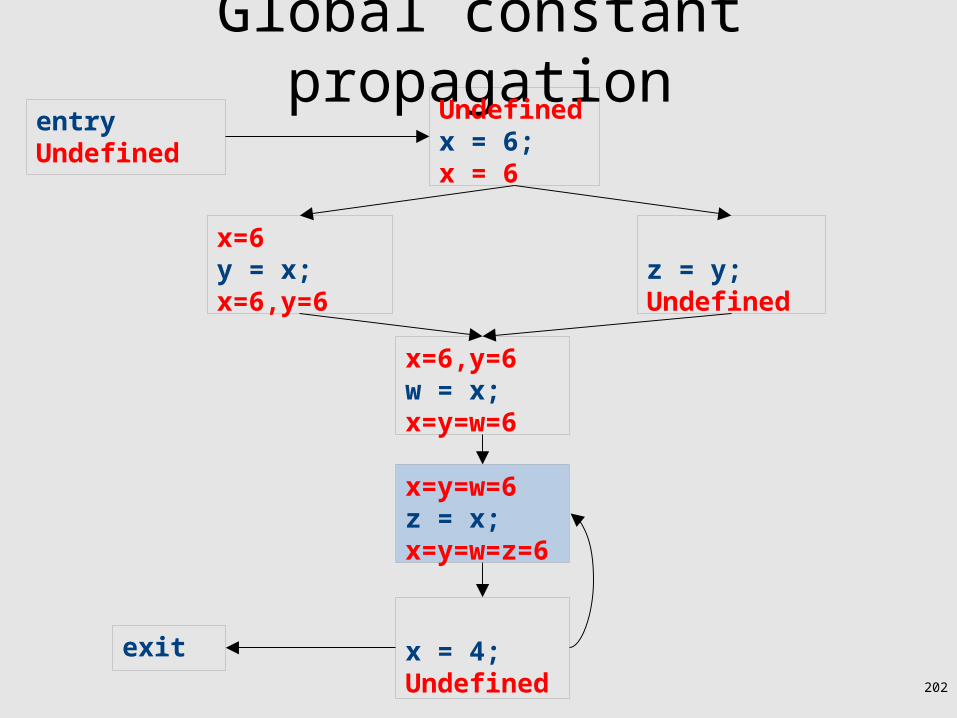
Global constant propagation
exit x = 4;Undefined
x=y=w=6z = x;x=y=w=z=6
x=6,y=6w = x;x=y=w=6
x=6y = x;x=6,y=6
z = y;Undefined
Undefinedx = 6;x = 6
entryUndefined
203
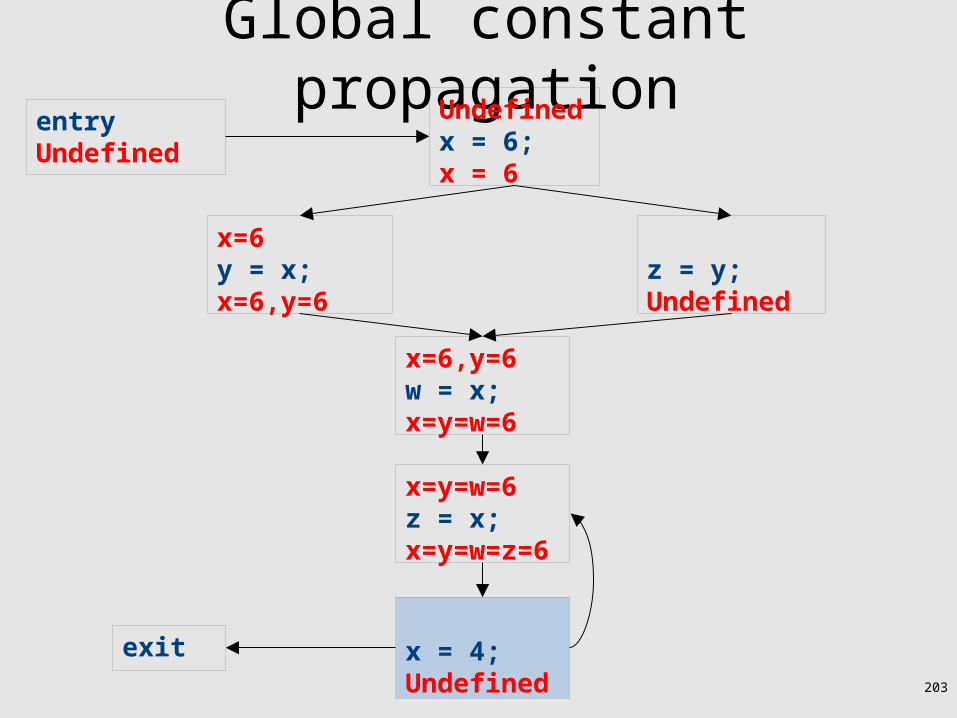
Global constant propagation
exit x = 4;Undefined
x=y=w=6z = x;x=y=w=z=6
x=6,y=6w = x;x=y=w=6
x=6y = x;x=6,y=6
z = y;Undefined
Undefinedx = 6;x = 6
entryUndefined

204
Global constant propagation
exitx=y=w=z=6x = 4;Undefined
x=y=w=6z = x;x=y=w=z=6
x=6,y=6w = x;x=y=w=6
x=6y = x;x=6,y=6
z = y;Undefined
Undefinedx = 6;x = 6
entryUndefined
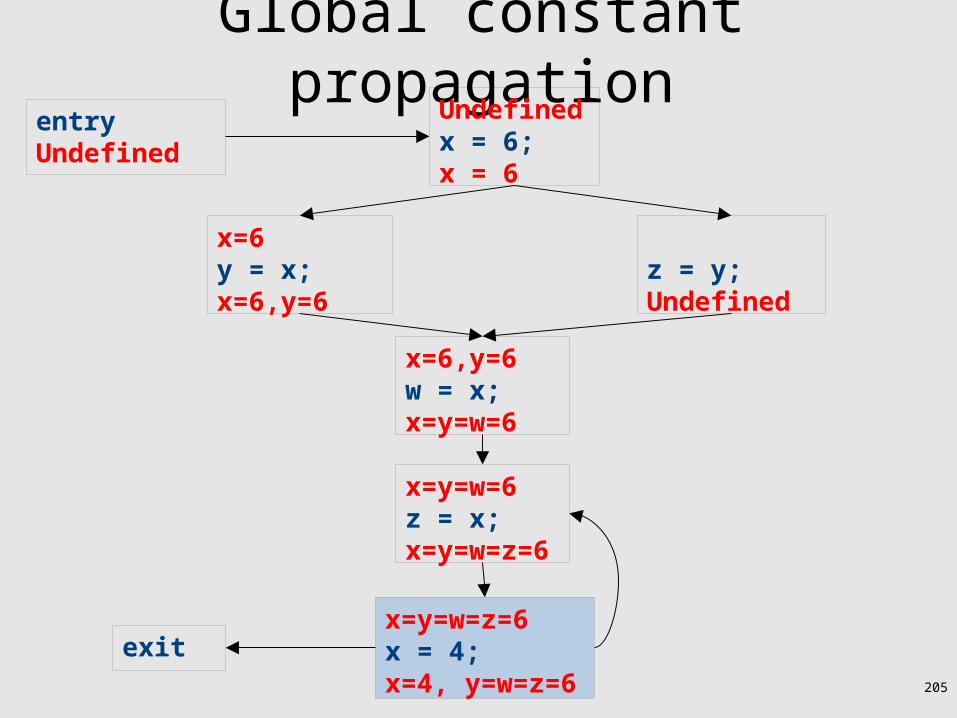
205
Global constant propagation
exitx=y=w=z=6x = 4;x=4, y=w=z=6
x=y=w=6z = x;x=y=w=z=6
x=6,y=6w = x;x=y=w=6
x=6y = x;x=6,y=6
z = y;Undefined
Undefinedx = 6;x = 6
entryUndefined
206
Global constant propagation
exitx=y=w=z=6x = 4;x=4, y=w=z=6
x=y=w=6z = x;x=y=w=z=6
x=6,y=6w = x;x=y=w=6
x=6y = x;x=6,y=6
z = y;Undefined
Undefinedx = 6;x = 6
entryUndefined

207
Global constant propagation
exitx=y=w=z=6x = 4;x=4, y=w=z=6
x=y=w=6z = x;x=y=w=z=6
x=6,y=6w = x;x=y=w=6
x=6y = x;x=6,y=6
x = 6z = y;Undefined
Undefinedx = 6;x = 6
entryUndefined

208
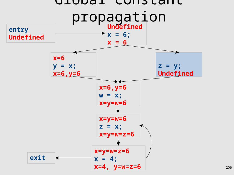
Global constant propagation
exitx=y=w=z=6x = 4;x=4, y=w=z=6
x=y=w=6z = x;x=y=w=z=6
x=6,y=6w = x;x=y=w=6
x=6y = x;x=6,y=6
x = 6z = y;Undefined
Undefinedx = 6;x = 6
entryUndefined
209
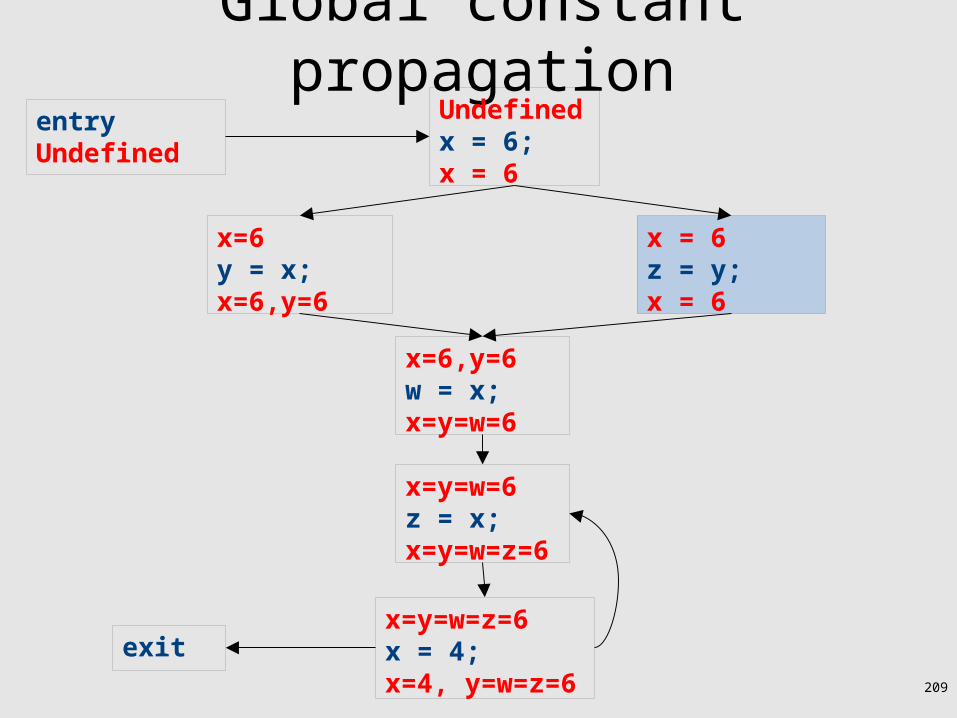
Global constant propagation
exitx=y=w=z=6x = 4;x=4, y=w=z=6
x=y=w=6z = x;x=y=w=z=6
x=6,y=6w = x;x=y=w=6
x=6y = x;x=6,y=6
x = 6z = y;x = 6
Undefinedx = 6;x = 6
entryUndefined
210
Global constant propagation
exitx=y=w=z=6x = 4;x=4, y=w=z=6
x=y=w=6z = x;x=y=w=z=6
x=6,y=6w = x;x=y=w=6
x=6y = x;x=6,y=6
x = 6z = y;x = 6
Undefinedx = 6;x = 6
entryUndefined
x=6 x=4 gives what?
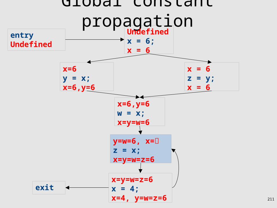
211
Global constant propagation
exitx=y=w=z=6x = 4;x=4, y=w=z=6
y=w=6, x=z = x;x=y=w=z=6
x=6,y=6w = x;x=y=w=6
x=6y = x;x=6,y=6
x = 6z = y;x = 6
Undefinedx = 6;x = 6
entryUndefined
212
Global constant propagation
exitx=y=w=z=6x = 4;x=4, y=w=z=6
y=w=6z = x;y=w=6
x=6,y=6w = x;x=y=w=6
x=6y = x;x=6,y=6
x = 6z = y;x = 6
Undefinedx = 6;x = 6
entryUndefined

213
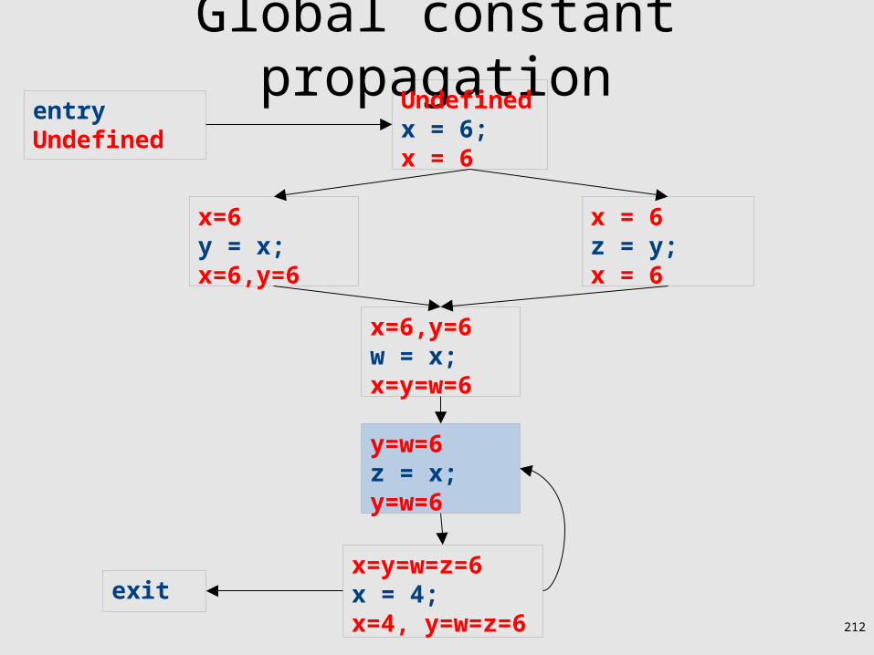
Global constant propagation
exitx=y=w=z=6x = 4;x=4, y=w=z=6
y=w=6z = x;y=w=6
x=6,y=6w = x;x=y=w=6
x=6y = x;x=6,y=6
x = 6z = y;x = 6
Undefinedx = 6;x = 6
entryUndefined

214
Global constant propagation
exity=w=6 x = 4;x=4, y=w=6
y=w=6z = x;y=w=6
x=6,y=6w = x;x=y=w=6
x=6y = x;x=6,y=6
x = 6z = y;x = 6
Undefinedx = 6;x = 6
entryUndefined
215
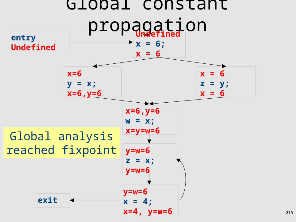
Global constant propagation
exity=w=6 x = 4;x=4, y=w=6
y=w=6z = x;y=w=6
x=6,y=6w = x;x=y=w=6
x=6y = x;x=6,y=6
x = 6z = y;x = 6
Undefinedx = 6;x = 6
entryUndefined
Global analysisreached fixpoint

216
Global constant propagation
exity=w=6x = 4;y=w=6
y=w=6z = x;y=w=6
x=6,y=6w = x;x=y=w=6
x=6y = x;x=6,y=6
x = 6z = y;x = 6
Undefinedx = 6;x = 6
entryUndefined

217
Global constant propagation
exity=w=6x = 4;y=w=6
y=w=6z = x;y=w=6
x=6,y=6w = 6;x=y=w=6
x=6y = 6;x=6,y=6
x = 6z = y;x = 6
Undefinedx = 6;x = 6
entryUndefined

218
Dataflow for constant propagation
• Direction: Forward• Semilattice: Vars {Undefined, 0, 1, -1, 2, -2, …, Not-a-
Constant}– Join mapping for variables point-wise
{x1,y1,z1} {x1,y2,zNot-a-Constant} = {x1,yNot-a-Constant,zNot-a-Constant}
• Transfer functions:– fx=k(V) = V|xk (update V by mapping x to k)– fx=a+b(V) = V|xNot-a-Constant (assign Not-a-Constant)
• Initial value: x is Undefined– (When might we use some other value?)

219
Proving termination
• Our algorithm for running these analyses continuously loops until no changes are detected
• Given this, how do we know the analyses will eventually terminate?– In general, we don‘t
220
Terminates?

221
Liveness Analysis
• A variable is live at a point in a program if later in the program its value will be read before it is written to again
222
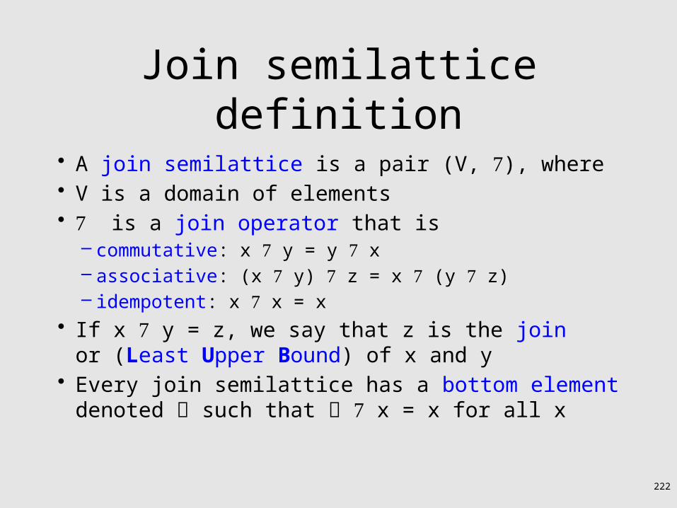
Join semilattice definition
• A join semilattice is a pair (V, ), where• V is a domain of elements• is a join operator that is
– commutative: x y = y x– associative: (x y) z = x (y z)– idempotent: x x = x
• If x y = z, we say that z is the joinor (Least Upper Bound) of x and y
• Every join semilattice has a bottom element denoted such that x = x for all x

223
Partial ordering induced by join
• Every join semilattice (V, ) induces an ordering relationship over its elements
• Define x y iff x y = y• Need to prove
– Reflexivity: x x– Antisymmetry: If x y and y x, then x = y– Transitivity: If x y and y z, then x z
224
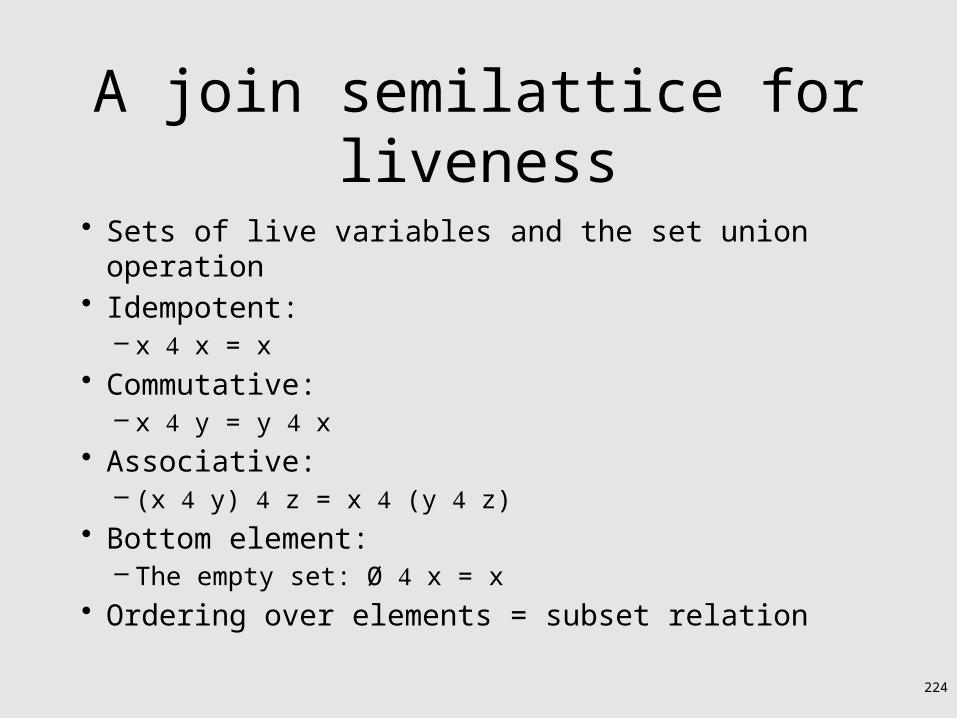
A join semilattice for liveness
• Sets of live variables and the set union operation• Idempotent:
– x x = x• Commutative:
– x y = y x• Associative:
– (x y) z = x (y z)• Bottom element:
– The empty set: Ø x = x• Ordering over elements = subset relation

225
Join semilattice example for liveness
{}
{a} {b} {c}
{a, b} {a, c} {b, c}
{a, b, c}
Bottom element

226
Dataflow framework
• A global analysis is a tuple (D, V, , F, I), where– D is a direction (forward or backward)
• The order to visit statements within a basic block,NOT the order in which to visit the basic blocks
– V is a set of values (sometimes called domain)– is a join operator over those values– F is a set of transfer functions fs : V V
(for every statement s)– I is an initial value
227
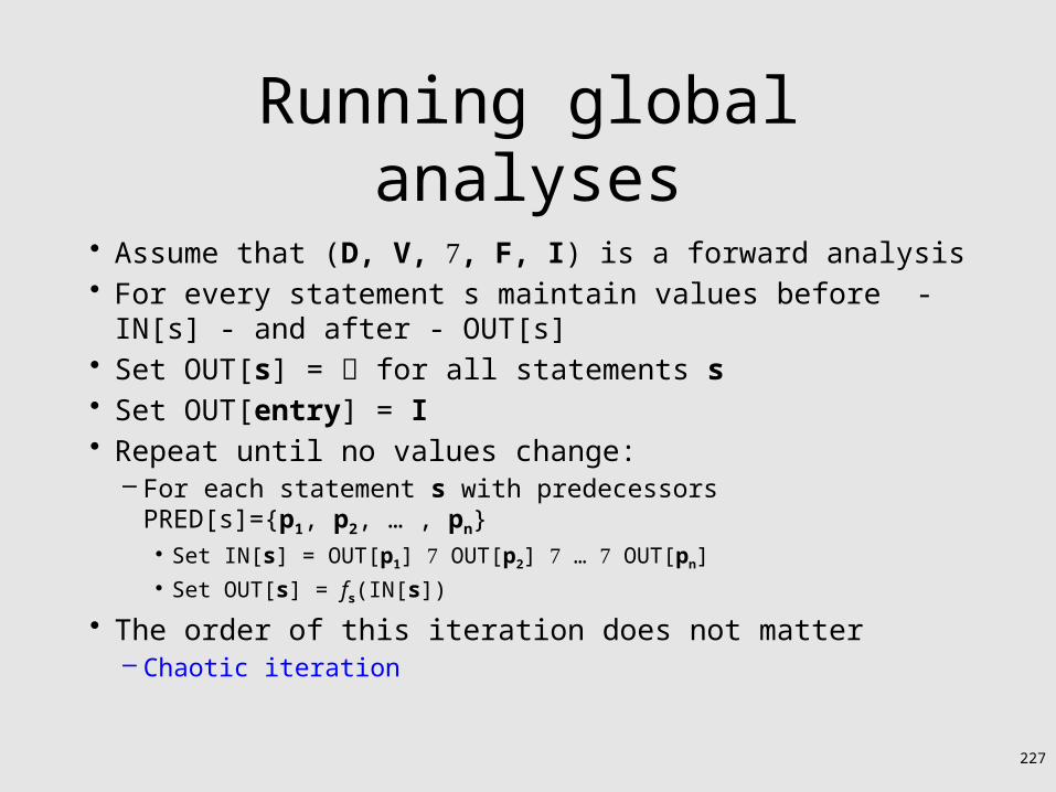
Running global analyses• Assume that (D, V, , F, I) is a forward analysis• For every statement s maintain values before - IN[s] - and after -
OUT[s]• Set OUT[s] = for all statements s• Set OUT[entry] = I• Repeat until no values change:
– For each statement s with predecessorsPRED[s]={p1, p2, … , pn}
• Set IN[s] = OUT[p1] OUT[p2] … OUT[pn]• Set OUT[s] = fs(IN[s])
• The order of this iteration does not matter– Chaotic iteration
228
Proving termination
• Our algorithm for running these analyses continuously loops until no changes are detected
• Problem: how do we know the analyses will eventually terminate?
229
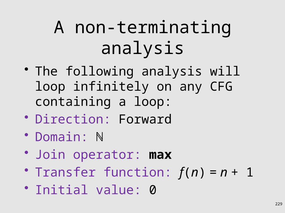
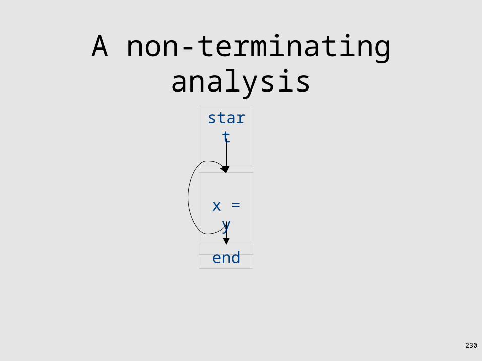
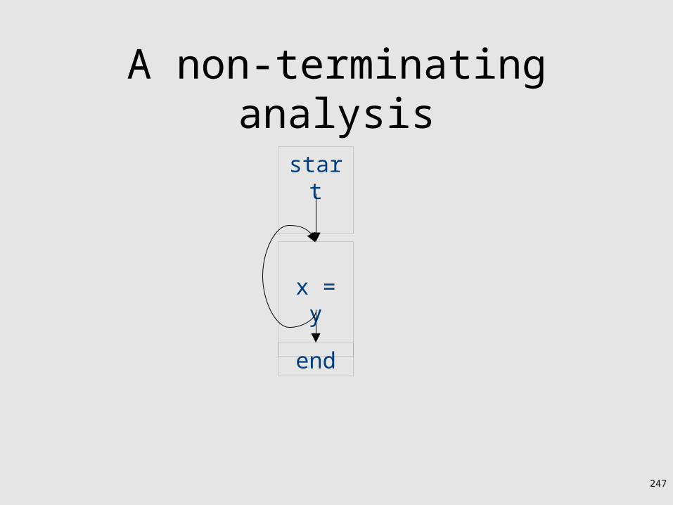
A non-terminating analysis
• The following analysis will loop infinitely on any CFG containing a loop:
• Direction: Forward• Domain: ℕ• Join operator: max• Transfer function: f(n) = n + 1• Initial value: 0
230
A non-terminating analysis
start
end
x = y
231
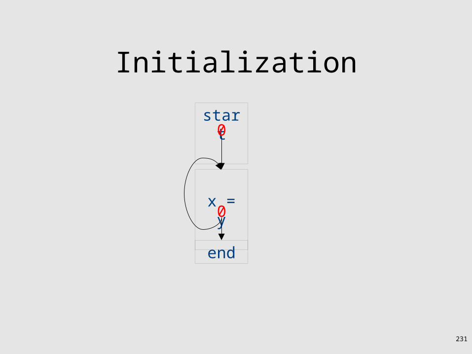
Initialization
start
end
x = y0
0
232
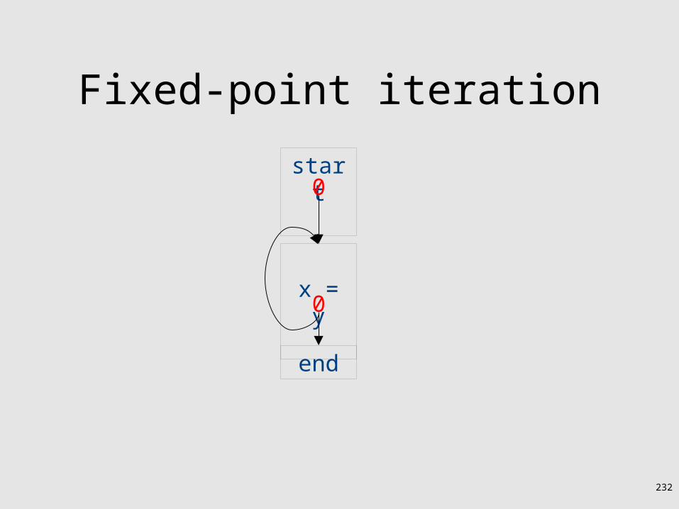
Fixed-point iteration
start
end
x = y0
0
233
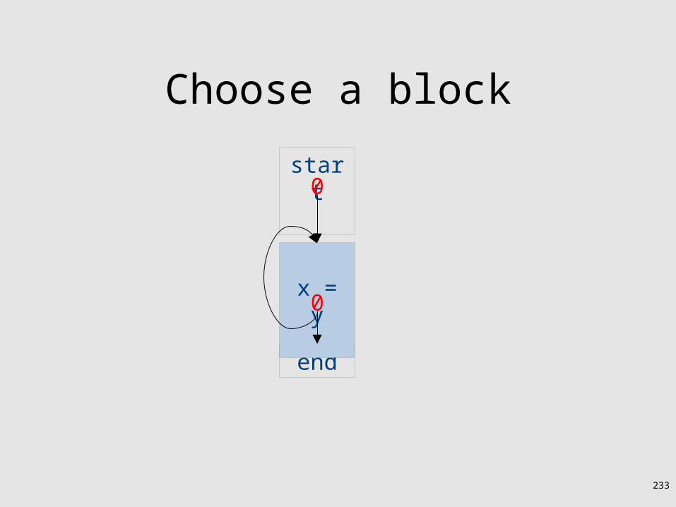
Choose a block
start
end
x = y0
0

234
Iteration 1
start
end
x = y0
0
0

235
Iteration 1
start
end
x = y1
0
0

236
Choose a block
start
end
x = y1
0
0

237
Iteration 2
start
end
x = y1
0
0

238
Iteration 2
start
end
x = y1
0
1

239
Iteration 2
start
end
x = y2
0
1

240
Choose a block
start
end
x = y2
0
1
241
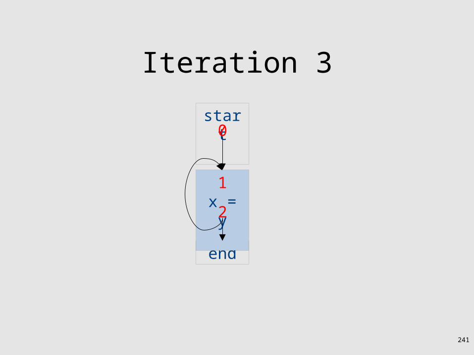
Iteration 3
start
end
x = y2
0
1

242
Iteration 3
start
end
x = y2
0
2

243
Iteration 3
start
end
x = y3
0
2
244
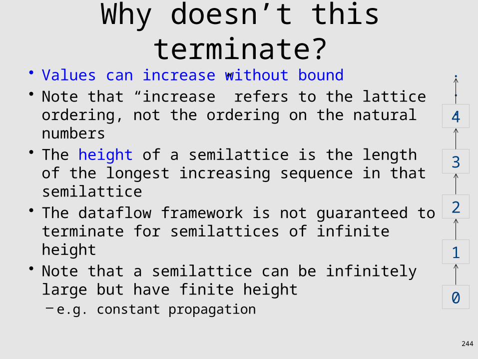
Why doesn’t this terminate?• Values can increase without bound• Note that “increase” refers to the lattice ordering,
not the ordering on the natural numbers• The height of a semilattice is the length of the
longest increasing sequence in that semilattice• The dataflow framework is not guaranteed to
terminate for semilattices of infinite height• Note that a semilattice can be infinitely large but
have finite height– e.g. constant propagation 0
1
2
3
4
...

245
Height of a lattice
• An increasing chain is a sequence of elements a1 a2 … ak
– The length of such a chain is k• The height of a lattice is the length of the maximal
increasing chain• For liveness with n program variables:
– {} {v1} {v1,v2} … {v1,…,vn}
• For available expressions it is the number of expressions of the form a=b op c– For n program variables and m operator types:
mn3

246
Another non-terminating analysis
• This analysis works on a finite-height semilattice, but will not terminate on certain CFGs:
• Direction: Forward• Domain: Boolean values true and false• Join operator: Logical OR• Transfer function: Logical NOT• Initial value: false
247
A non-terminating analysis
start
end
x = y

248
Initialization
start
end
x = yfalse
false
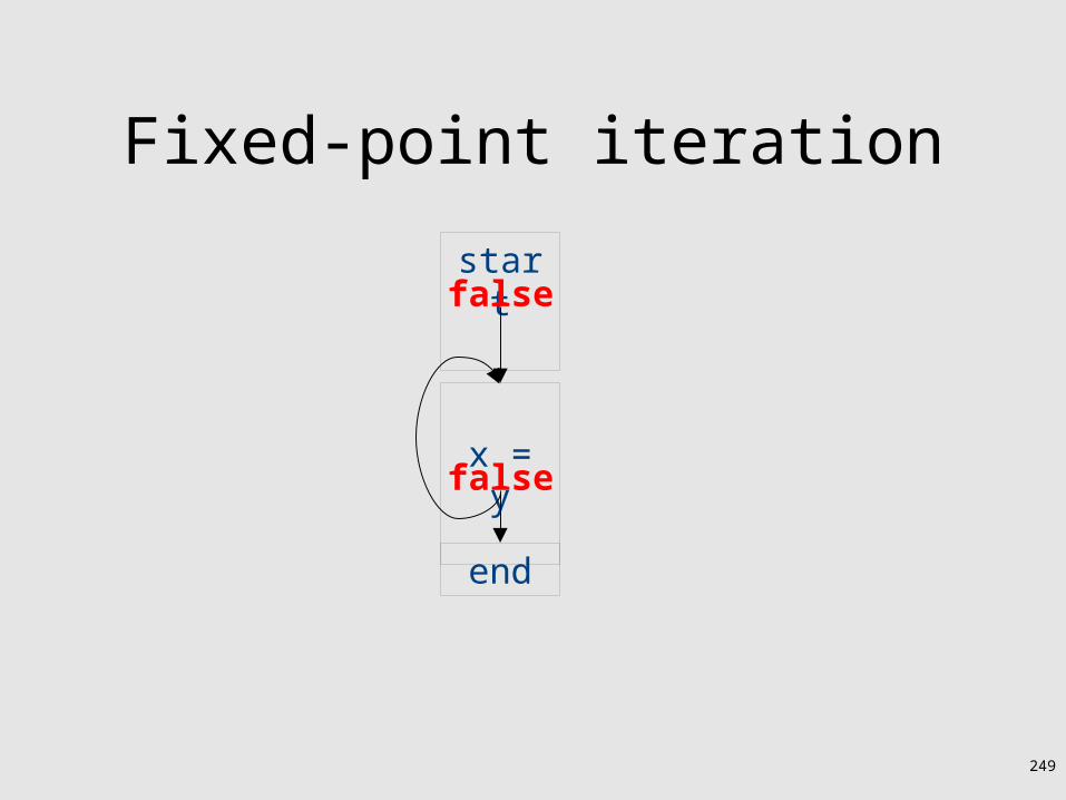
249
Fixed-point iteration
start
end
x = yfalse
false
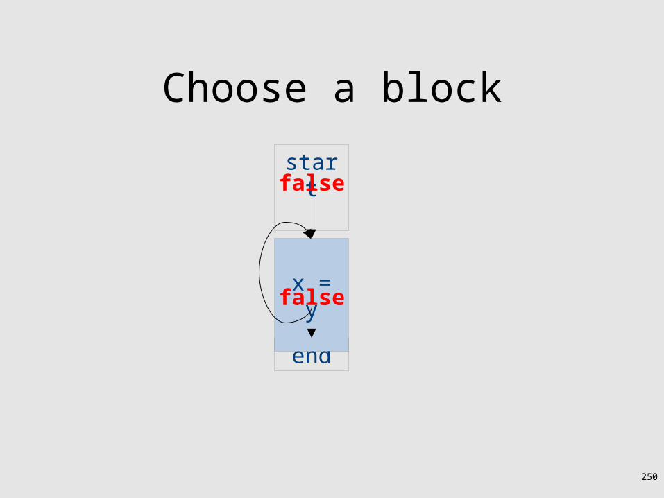
250
Choose a block
start
end
x = yfalse
false

251
Iteration 1
start
end
x = yfalse
false
false
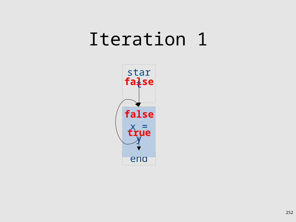
252
Iteration 1
start
end
x = ytrue
false
false

253
Iteration 2
start
end
x = ytrue
false
true

254
Iteration 2
start
end
x = yfalse
false
true

255
Iteration 3
start
end
x = yfalse
false
false
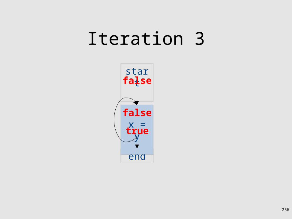
256
Iteration 3
start
end
x = ytrue
false
false
257
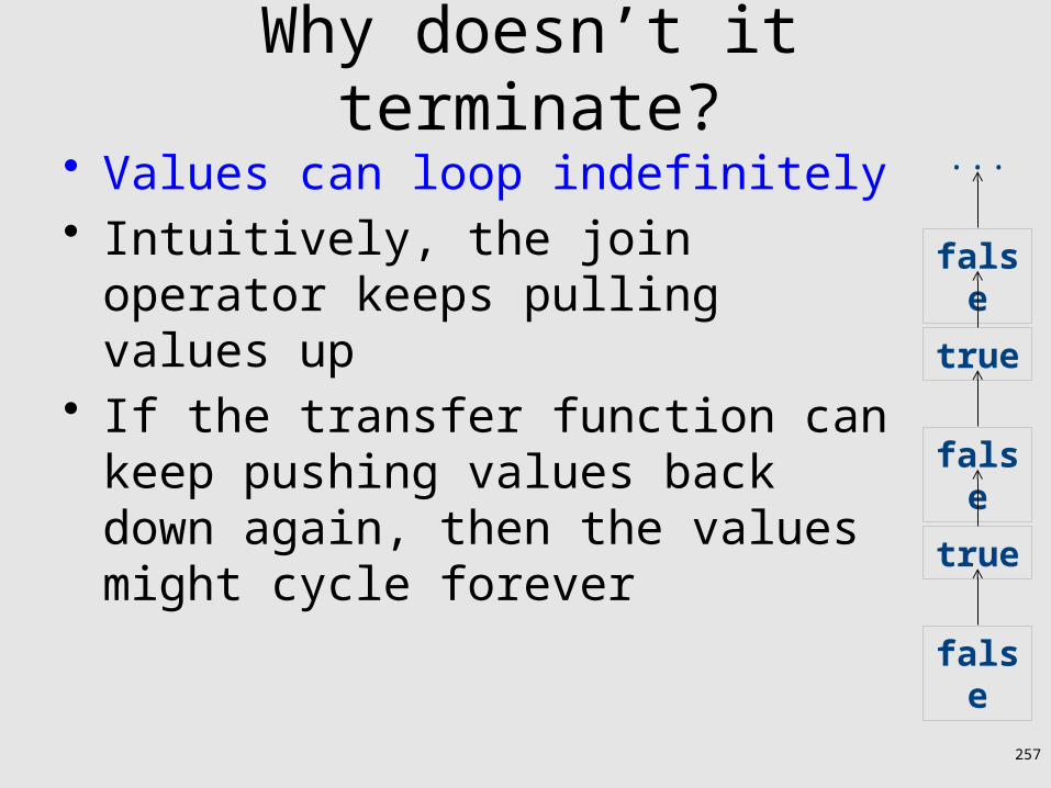
Why doesn’t it terminate?• Values can loop indefinitely• Intuitively, the join operator keeps pulling
values up• If the transfer function can keep pushing
values back down again, then the values might cycle forever
false
true
false
true
false
...

258
Why doesn’t it terminate?• Values can loop indefinitely• Intuitively, the join operator keeps pulling
values up• If the transfer function can keep pushing
values back down again, then the values might cycle forever
• How can we fix this?
false
true
false
true
false
...

259
Monotone transfer functions
• A transfer function f is monotone iff if x y, then f(x) f(y)
• Intuitively, if you know less information about a program point, you can't “gain back” more information about that program point
• Many transfer functions are monotone, including those for liveness and constant propagation
• Note: Monotonicity does not mean that x f(x)– (This is a different property called extensivity)
260
Liveness and monotonicity
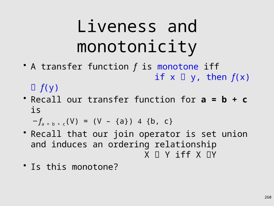
• A transfer function f is monotone iff if x y, then f(x) f(y)
• Recall our transfer function for a = b + c is– fa = b + c(V) = (V – {a}) {b, c}
• Recall that our join operator is set union and induces an ordering relationship X Y iff X Y
• Is this monotone?

261
Is constant propagation monotone?• A transfer function f is monotone iff
if x y, then f(x) f(y)• Recall our transfer functions
– fx=k(V) = V|xk (update V by mapping x to k)– fx=a+b(V) = V|xNot-a-Constant (assign Not-a-Constant)
• Is this monotone?
Undefined
0-1-2 1 2 ......
Not-a-constant
262
The grand result
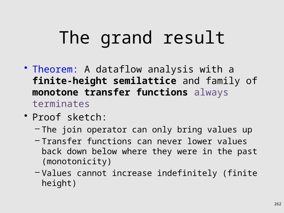
• Theorem: A dataflow analysis with a finite-height semilattice and family of monotone transfer functions always terminates
• Proof sketch:– The join operator can only bring values up– Transfer functions can never lower values back
down below where they were in the past (monotonicity)
– Values cannot increase indefinitely (finite height)

263
An “optimality” result
• A transfer function f is distributive if f(a b) = f(a) f(b)for every domain elements a and b
• If all transfer functions are distributive then the fixed-point solution is the solution that would be computed by joining results from all (potentially infinite) control-flow paths– Join over all paths
• Optimal if we ignore program conditions

264
An “optimality” result
• A transfer function f is distributive if f(a b) = f(a) f(b)for every domain elements a and b
• If all transfer functions are distributive then the fixed-point solution is equal to the solution computed by joining results from all (potentially infinite) control-flow paths– Join over all paths
• Optimal if we pretend all control-flow paths can be executed by the program
• Which analyses use distributive functions?
265
Loop optimizations
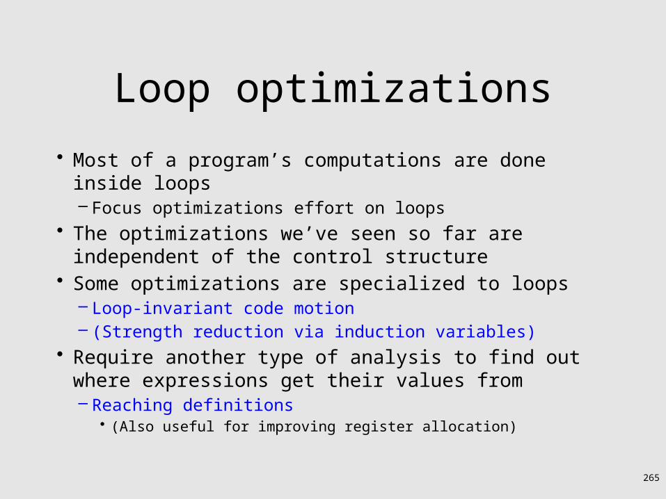
• Most of a program’s computations are done inside loops– Focus optimizations effort on loops
• The optimizations we’ve seen so far are independent of the control structure
• Some optimizations are specialized to loops– Loop-invariant code motion– (Strength reduction via induction variables)
• Require another type of analysis to find out where expressions get their values from– Reaching definitions
• (Also useful for improving register allocation)

266
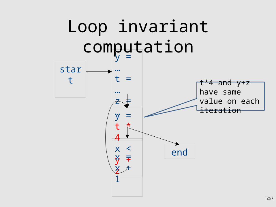
Loop invariant computation
y = t * 4x < y + z endx = x + 1
starty = …t = …z = …
267
Loop invariant computation
y = t * 4x < y + z endx = x + 1
starty = …t = …z = …
t*4 and y+zhave same value on each iteration

268
Code hoisting
x < w
endx = x + 1
starty = …t = …z = …y = t * 4w = y + z

269
What reasoning did we use?
y = t * 4x < y + z endx = x + 1
starty = …t = …z = …
y is defined inside loop but it is loop invariant since t*4 is loop-invariant
Both t and z are defined only outside of loop
constants are trivially loop-invariant
270
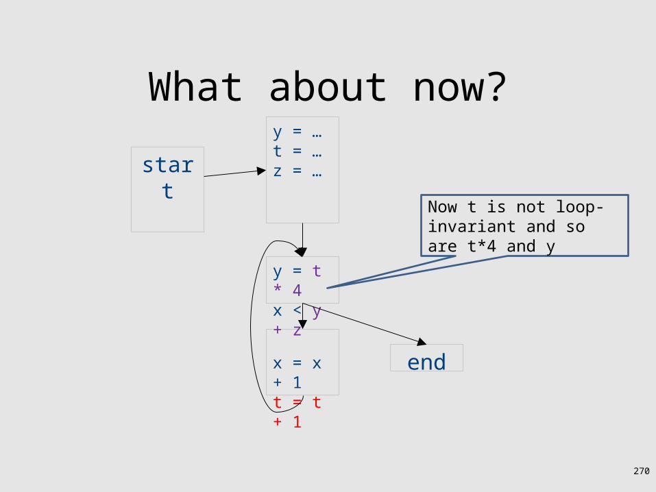
What about now?
y = t * 4x < y + z
endx = x + 1t = t + 1
start
y = …t = …z = …
Now t is not loop-invariant and so are t*4 and y
271
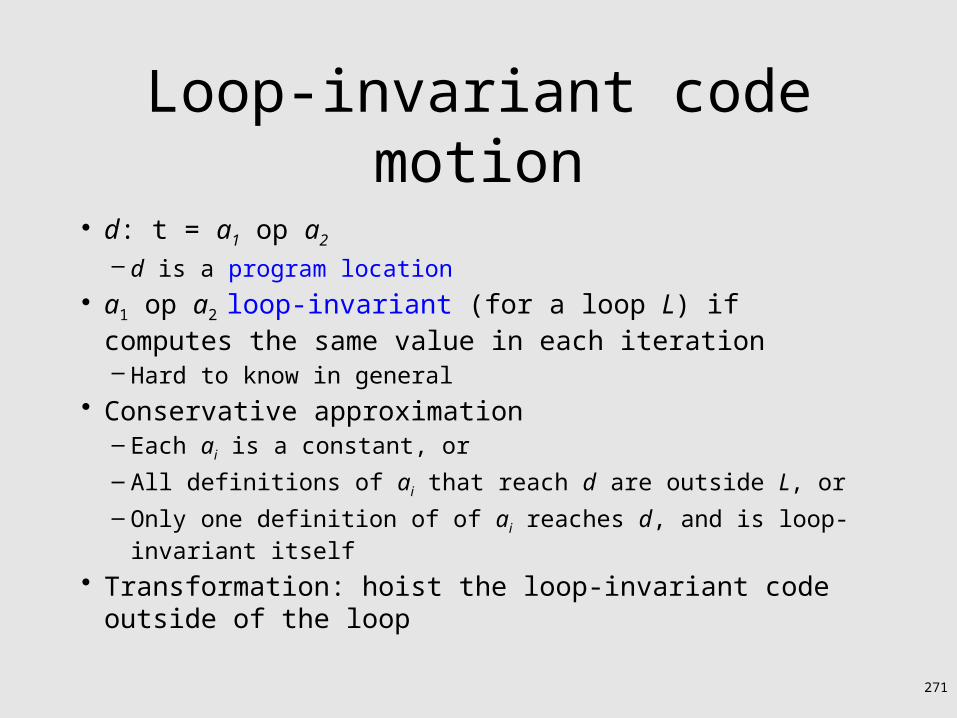
Loop-invariant code motion
• d: t = a1 op a2
– d is a program location• a1 op a2 loop-invariant (for a loop L) if computes the same value
in each iteration– Hard to know in general
• Conservative approximation– Each ai is a constant, or– All definitions of ai that reach d are outside L, or– Only one definition of of ai reaches d, and is loop-invariant itself
• Transformation: hoist the loop-invariant code outside of the loop

272
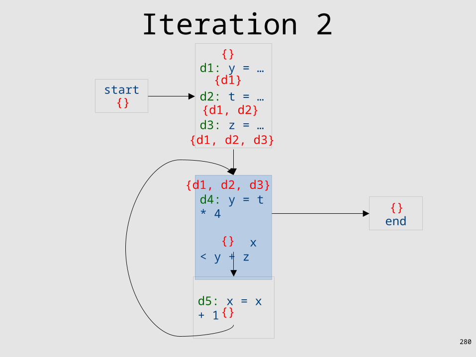
Reaching definitions analysis• A definition d: t = … reaches a program location if there is a path from
the definition to the program location, along which the defined variable is never redefined

273
Reaching definitions analysis• A definition d: t = … reaches a program location if there is a path
from the definition to the program location, along which the defined variable is never redefined
• Direction: Forward• Domain: sets of program locations that are definitions `• Join operator: union• Transfer function:
fd: a=b op c(RD) = (RD - defs(a)) {d} fd: not-a-def(RD) = RD– Where defs(a) is the set of locations defining a (statements of the form
a=...)• Initial value: {}

274
Reaching definitions analysis
d4: y = t * 4
d4:x < y + z
d6: x = x + 1
d1: y = …
d2: t = …
d3: z = …
start
end{}

275
Reaching definitions analysis
d4: y = t * 4
d4:x < y + z
d5: x = x + 1
start
d1: y = …
d2: t = …
d3: z = …
end{}

276
Initialization
d4: y = t * 4
d4:x < y + z
d5: x = x + 1
start
d1: y = …
d2: t = …
d3: z = …
{}
{}
{}
{}
end{}

277
Iteration 1
d4: y = t * 4
d4:x < y + z
d5: x = x + 1
start
d1: y = …
d2: t = …
d3: z = …
{}
{}
{}
{}
end{}
{}

278
Iteration 1
d4: y = t * 4
d4:x < y + z
d5: x = x + 1
start
d1: y = …
d2: t = …
d3: z = …
{}
{}
{d1}
{d1, d2}
{d1, d2, d3}
end{}
{}
{}

279
Iteration 2
d4: y = t * 4
x < y + z end
d5: x = x + 1
start
d1: y = …
d2: t = …
d3: z = …
{}
{}
{}
{d1}
{d1, d2}
{d1, d2, d3}
{}
{}
280
Iteration 2
d4: y = t * 4
x < y + z end
d5: x = x + 1
start
d1: y = …
d2: t = …
d3: z = …
{}
{}
{d1, d2, d3}
{}
{d1}
{d1, d2}
{d1, d2, d3}
{}
{}
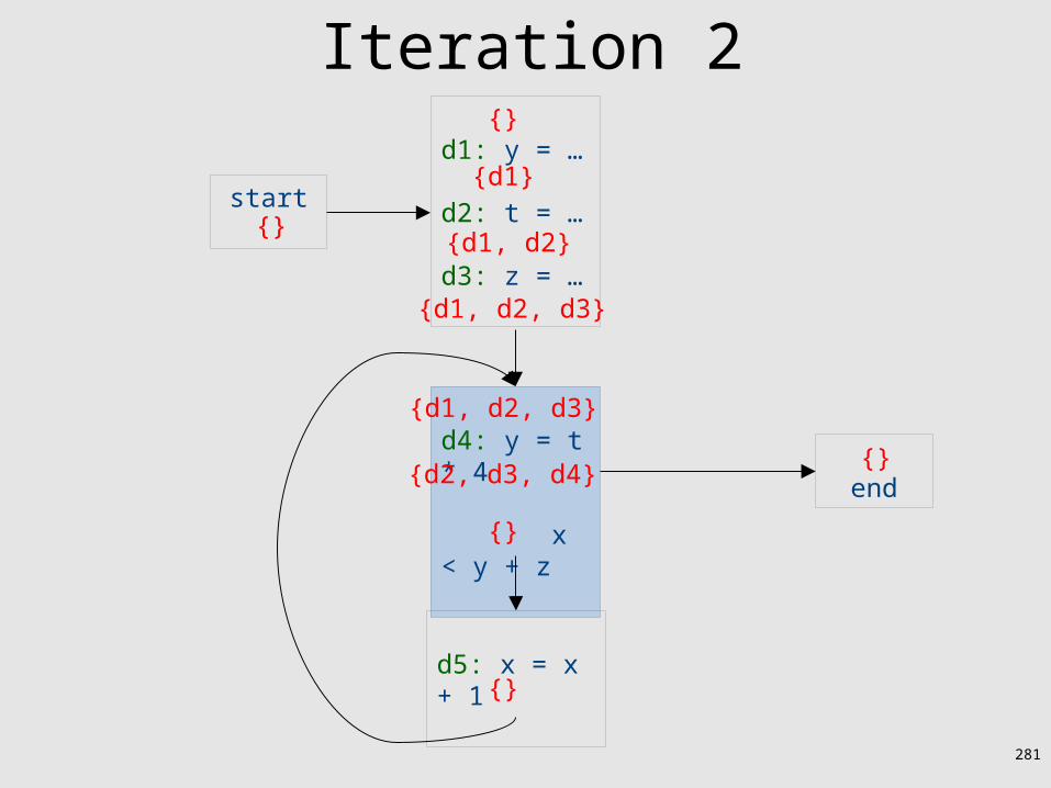
281
Iteration 2
d4: y = t * 4
x < y + z end
d5: x = x + 1
start
d1: y = …
d2: t = …
d3: z = …
{}
{}
{d1, d2, d3}
{}
{d1}
{d1, d2}
{d1, d2, d3}
{d2, d3, d4}
{}
{}

282
Iteration 2
d4: y = t * 4
x < y + z end
d5: x = x + 1
start
d1: y = …
d2: t = …
d3: z = …
{}
{}
{d1, d2, d3}
{}
{d1}
{d1, d2}
{d1, d2, d3}
{d2, d3, d4}
{d2, d3, d4}
{}

283
Iteration 3
d4: y = t * 4
x < y + z end
d5: x = x + 1
start
d1: y = …
d2: t = …
d3: z = …
{}
{}
{d1, d2, d3}
{d2, d3, d4}
{}
{d1}
{d1, d2}
{d1, d2, d3}
{d2, d3, d4}
{d2, d3, d4}
{}

284
Iteration 3
d4: y = t * 4
x < y + z end
d5: x = x + 1
start
d1: y = …
d2: t = …
d3: z = …
{}
{}
{d1, d2, d3}
{d2, d3, d4}
{}
{d1}
{d1, d2}
{d1, d2, d3}
{d2, d3, d4}
{d2, d3, d4}
{d2, d3, d4, d5}

285
Iteration 4
d4: y = t * 4
x < y + z end
d5: x = x + 1
start
d1: y = …
d2: t = …
d3: z = …
{}
{}
{d1, d2, d3}
{d2, d3, d4}
{}
{d1}
{d1, d2}
{d1, d2, d3}
{d2, d3, d4}
{d2, d3, d4}
{d2, d3, d4, d5}

286
Iteration 4
d4: y = t * 4
x < y + z end
d5: x = x + 1
start
d1: y = …
d2: t = …
d3: z = …
{}
{}
{d1, d2, d3, d4, d5}
{d2, d3, d4}
{}
{d1}
{d1, d2}
{d1, d2, d3}
{d2, d3, d4}
{d2, d3, d4}
{d2, d3, d4, d5}

287
Iteration 4
d4: y = t * 4
x < y + z end
d5: x = x + 1
start
d1: y = …
d2: t = …
d3: z = …
{}
{}
{d1, d2, d3, d4, d5}
{d2, d3, d4}
{}
{d1}
{d1, d2}
{d1, d2, d3}
{d2, d3, d4, d5}
{d2, d3, d4, d5}
{d2, d3, d4, d5}

288
Iteration 5
end
start
d1: y = …
d2: t = …
d3: z = …
{}
{}
{d2, d3, d4, d5}
{d1}
{d1, d2}
{d1, d2, d3}
d5: x = x + 1{d2, d3, d4}
{d2, d3, d4, d5}
d4: y = t * 4
x < y + z
{d1, d2, d3, d4, d5}
{d2, d3, d4, d5}
{d2, d3, d4, d5}

289
Iteration 6
end
start
d1: y = …
d2: t = …
d3: z = …
{}
{}
{d2, d3, d4, d5}
{d1}
{d1, d2}
{d1, d2, d3}
d5: x = x + 1{d2, d3, d4, d5}
{d2, d3, d4, d5}
d4: y = t * 4
x < y + z
{d1, d2, d3, d4, d5}
{d2, d3, d4, d5}
{d2, d3, d4, d5}

290
Which expressions are loop invariant?
t is defined only in d2 – outside of loop
z is defined only in d3 – outside of loop
y is defined only in d4 – inside of loop but depends on t and 4, both loop-invariant
start
d1: y = …
d2: t = …
d3: z = …
{}
{}
{d1}
{d1, d2}
{d1, d2, d3}
end{d2, d3, d4, d5}
d5: x = x + 1{d2, d3, d4, d5}
{d2, d3, d4, d5}
d4: y = t * 4
x < y + z
{d1, d2, d3, d4, d5}
{d2, d3, d4, d5}
{d2, d3, d4, d5}x is defined only in d5 – inside of loop so is not a loop-invariant

291
Inferring loop-invariant expressions
• For a statement s of the form t = a1 op a2
• A variable ai is immediately loop-invariant if all reaching definitions IN[s]={d1,…,dk} for ai are outside of the loop
• LOOP-INV = immediately loop-invariant variables and constantsLOOP-INV = LOOP-INV {x | d: x = a1 op a2, d is in the loop, and both a1 and a2 are in LOOP-INV}– Iterate until fixed-point
• An expression is loop-invariant if all operands are loop-invariants

292
Computing LOOP-INV
end
start
d1: y = …
d2: t = …
d3: z = …
{}
{}
{d2, d3, d4}
{d1}
{d1, d2}
{d1, d2, d3}
d4: y = t * 4
x < y + z
d5: x = x + 1
{d1, d2, d3, d4, d5}
{d2, d3, d4, d5}
{d2, d3, d4, d5}
{d2, d3, d4, d5}
{d2, d3, d4, d5}

293
Computing LOOP-INV
end
start
d1: y = …
d2: t = …
d3: z = …
{}
{}
{d2, d3, d4}
{d1}
{d1, d2}
{d1, d2, d3}
d4: y = t * 4
x < y + z
d5: x = x + 1
{d1, d2, d3, d4, d5}
{d2, d3, d4, d5}
{d2, d3, d4, d5}
{d2, d3, d4, d5}
{d2, d3, d4, d5}
(immediately)LOOP-INV = {t}

294
Computing LOOP-INV
end
start
d1: y = …
d2: t = …
d3: z = …
{}
{}
{d2, d3, d4}
{d1}
{d1, d2}
{d1, d2, d3}
d4: y = t * 4
x < y + z
d5: x = x + 1
{d1, d2, d3, d4, d5}
{d2, d3, d4, d5}
{d2, d3, d4, d5}
{d2, d3, d4, d5}
{d2, d3, d4, d5}
(immediately)LOOP-INV = {t, z}

295
Computing LOOP-INV
end
start
d1: y = …
d2: t = …
d3: z = …
{}
{}
{d2, d3, d4}
{d1}
{d1, d2}
{d1, d2, d3}
d4: y = t * 4
x < y + z
d5: x = x + 1
{d1, d2, d3, d4, d5}
{d2, d3, d4, d5}
{d2, d3, d4, d5}
{d2, d3, d4, d5}
{d2, d3, d4, d5}
(immediately)LOOP-INV = {t, z}

296
Computing LOOP-INV
end
start
d1: y = …
d2: t = …
d3: z = …
{}
{}
{d2, d3, d4}
{d1}
{d1, d2}
{d1, d2, d3}
d4: y = t * 4
x < y + z
d5: x = x + 1
{d1, d2, d3, d4, d5}
{d2, d3, d4, d5}
{d2, d3, d4, d5}
{d2, d3, d4, d5}
{d2, d3, d4, d5}
(immediately)LOOP-INV = {t, z}
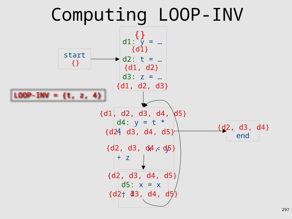
297
end
start
d1: y = …
d2: t = …
d3: z = …
{}
{}
{d2, d3, d4}
{d1}
{d1, d2}
{d1, d2, d3}LOOP-INV = {t, z, 4}
d4: y = t * 4
x < y + z
d5: x = x + 1
{d1, d2, d3, d4, d5}
{d2, d3, d4, d5}
{d2, d3, d4, d5}
{d2, d3, d4, d5}
{d2, d3, d4, d5}
Computing LOOP-INV
298
Computing LOOP-INV
d4: y = t * 4
x < y + z end
d5: x = x + 1
start
d1: y = …
d2: t = …
d3: z = …
{}
{}
{d1, d2, d3, d4, d5}
{d2, d3, d4, d5}
{d2, d3, d4}
{d1}
{d1, d2}
{d1, d2, d3}
{d2, d3, d4, d5}
{d2, d3, d4, d5}
{d2, d3, d4, d5}
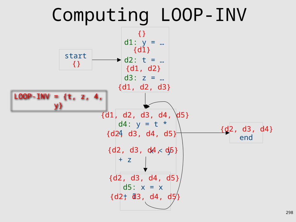
LOOP-INV = {t, z, 4, y}
299
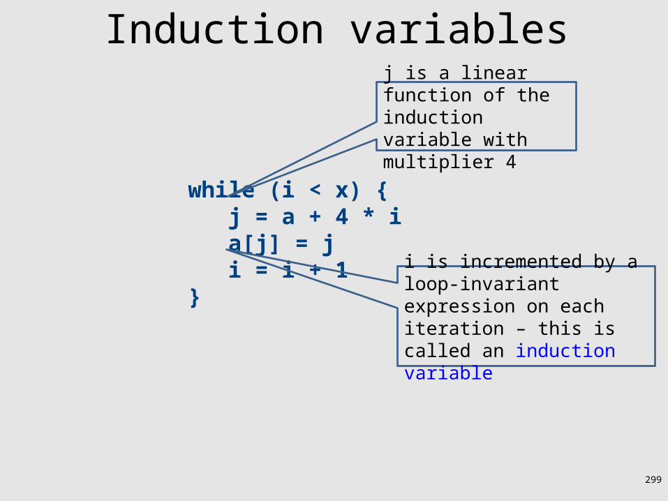
Induction variables
while (i < x) { j = a + 4 * i a[j] = j i = i + 1}
i is incremented by a loop-invariant expression on each iteration – this is called an induction variable
j is a linear function of the induction variable with multiplier 4

300
Strength-reduction
j = a + 4 * i while (i < x) { j = j + 4 a[j] = j i = i + 1}
Prepare initial value
Increment by multiplier
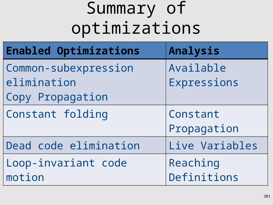
301
Summary of optimizations
Enabled Optimizations AnalysisCommon-subexpression eliminationCopy Propagation
Available Expressions
Constant folding Constant PropagationDead code elimination Live VariablesLoop-invariant code motion Reaching Definitions
Top Related