


Languages
Pages
Legal

Horner, Bonnie L. 2008. Comparison of Population Distribution Models using Areal Interpolation with
Incompatible Spatial Zones. Volume 11. Papers in Resource Analysis. 15 pp. Saint Mary’s University of Minnesota
University Central Services Press. Winona, MN Retrieved (date) http:/www.gis.smumn.edu
Comparison of Population Distribution Models using Areal Interpolation on Data with
Incompatible Spatial Zones
Bonnie L Horner
Department of Resource Analysis, Saint Mary’s University of Minnesota, Minneapolis, MN
55404
Keywords: GIS, Interpolation, Population, Dasymetric, Zip Codes
Abstract
Population data is collected by the government and released in census spatial zones as aggregate
counts. The key problem in using this valuable dataset is the need to reassign the data to other
geographical areas when the geographical zonal systems are incompatible. Areal interpolation is
used to dis-aggregate census data into areas or zones that are compatible and can be analyzed. In
this project, two population distribution models are compared using areal interpolation. The two
distribution models evaluated consist of simple areal weighting and a dasymetric-based
approach. Simple areal weighting is used with 2000 census data in various zip code areas. The
dasymetric approach uses the Hennepin County, MN parcels to redistribute the same 2000
census data. The analysis is conducted using a five mile radius around a new hospital site in
Hennepin County, MN. The proposed output of this study concludes that dasymetric areal
interpolation of population is more representative of actual density than simple areal weighting.
Introduction
Population estimates are critical for many
spatial analysis tasks in government, urban
planning, criminology, research and
marketing. Government instigated national
censuses (i.e. US Census) are the foundation
for most geodemographic analysis. This
census data offers the most accurate and
nationally complete record of both
geographical patterns and socio-economic
characteristics of population (Langford et
al., 2006).
Census data is not available in point-
to-point format. Due to confidentiality
requirements and to reduce data volumes,
this information is available only as
aggregate values. The smallest spatial zone
of aggregate data is the census block group.
Population mapping most commonly
displays population data as evenly
distributed within the census enumeration
area (Holt et al., 2004). Population density
is shown to be the same throughout the
zones with abrupt population changes at the
zone boundaries. However, population is
continuous and does not follow boundaries.
Additionally, population in urban areas is
more dense than population in rural areas.
GIS is a great tool to use with
population analysis. One of the key
strengths of GIS is the ability to integrate
data from one incompatible spatial zone to
another spatial zone and then, to perform
spatial analysis on the spatial zone. GIS can
also utilize large or multiple datasets and
create smaller manageable datasets to use
for analysis or areal interpolation.
Intersection of datasets or spatial buffers can
also be joined to ancillary data to help
interpret the results of the newly created
datasets.
In this study, two population
distribution models were used to perform
areal interpolation and analyze population
counts. Zip code areas are used to represent

2
simple areal weighting. This is compared to
dasymetric interpolation. The dasymetric
interpolation uses county parcels as the
ancillary data to redistribute population
counts within census blocks. In this study a
buffer was created around a hospital in the
city of Maple Grove study area (Figure 1).
The results of the two models are then
descriptively compared.
Figure 1. Hospital site and ten zip code study area.
One inch = 4 miles.
Areal Interpolation
One method of determining population
distribution is through areal interpolation.
Areal interpolation refers to interpolation
using polygons or “areas.” Areal
interpolation transfers data into a common
dataset for use in analysis and comparison
(Mennis, 2003). The two types of
interpolation that are used in this study are
the simple areal weighting and a dasymetric-
based interpolation method.
Population Distribution Models
Simple Areal Weighting
Simple areal interpolation is the simplest
approach to spatially distribute population
counts. This process distributes the
population count evenly within the limits of
the zone boundaries studied. This
distribution, however, does not represent the
actual distribution of population. Population
is not evenly distributed within the
boundary, but population is continuous. This
even-distribution of population over
estimates or distorts the data within each
unit/block (Holt et al., 2004). In reality,
population would be concentrated within
multi-family or apartments over single
family housing, and urban areas over rural
areas. Simple areal weighting does give
commercial, industrial and public lands a
population value. In reality, these areas do
not have population.
Simple areal weighting is often
mapped in the form of choropleth maps.
Choropleth maps display the values
distributed in each block as color blocks.
Each different value has a distinct color.
In Figure 2, the 55311 zip code has a
total population of 19,827. The total area of
zip code 55311 is 13,793.82 acres.
Density = Total population / Total acres
According to simple areal weighting, the
density in this zip code is 19827 / 13,793.82
or 1.44 people per acre.
Dasymetric Interpolation
The dasymetric approach to areal
interpolation is an area based approach to
interpolation (Holt et al., 2004). It uses
ancillary information to determine the
distribution of the chosen variable. The
ancillary or additional data could be land-
use/land-cover data or census data. Ancillary
data further refines data inside boundaries
into more accurate zones of internal

3
Figure 2. Zip Code 55311. One inch = 5 miles.
homogeneity (Eicher and Brewer, 2001).
Dasymetric mapping was first
popularized in the United States by John
Wright (1936). Wright used ancillary data to
distribute population data into
populated/unpopulated areas and mapped
the results.
With computers and GIS, the ability
to use ancillary data has become easier.
Dasymetric mapping has the ability to
achieve a more thorough representation of
the underlying geography. Dasymetric maps
create zones of internal homogeneity and
reflect the spatial distribution of the variable
being mapped. It removes the abrupt zone
changes of the simple areal interpolation by
redistributing the data according to the
ancillary data into the target zones to be
analyzed. Most ancillary data used in this
method consists of land use data derived
from satellite imagery (Mennis, 2003). Land
use data divides the areas into
populated/unpopulated and population is
distributed accordingly.
In this study, parcels are the ancillary
data to be used to distribute the population
counts by the dasymetric method. The parcel
use-description attribute is used to
interpolate population into categories for
analysis.
Figure 3 illustrates parcels within the
zip code area of 55311. The parcels are
given a value according to their parcel type.
The parcel types are commercial, duplex,
condo/townhouse and single family/farm.
Figure 3. Parcel types of zip code area 55311. One
inch = 5 miles.
US Census
The first US Census was taken in 1790. The
US constitution mandates that the Census of
Population and Housing be completed every
ten years to apportion seats in the House of
Representatives. Over the years, the census
has grown in size and function. It is the
world’s oldest continuous national census
(Peters and MacDonald, 2004). Census data
is released as aggregate counts and statistics
for corresponding zones. This is due to the
legal requirement to maintain confidentiality
of the individuals and it also aids in
controlling data volume (Langford, 2004).
Census data is stored as polygons or
areal units and contain demographical data
such as average household size, family
households, income, household status and

4
children (Mennis, 2003). The data is broken
down from largest to smallest geography
units as follows: nation, region, division,
state, counties, census tracts, block groups,
and finally into census blocks. The block
group is the smallest spatial unit for which
there is sample data available. The
boundaries of census zones are arbitrary and
can change from one census to another (Cai,
2006).
In research, the spatial zones
required for an analysis rarely follow census
zones (Langsford, 2004). Additionally,
various agencies such as schools, retail, and
government that report information create
their own administrative boundaries. These
boundaries can change over time as do the
census boundaries. Using GIS for analysis
can create additional analytical zones such
as those of buffers, overlays and viewshed
analyses. The solution to integrate
incompatible spatial zones into zones that
are compatible is to transform the data using
area interpolation techniques into
compatible spatial zones (Langford, 2004).
Zip Codes
US zip codes are one of the “quirkier
geographies” in the world. The idea of
partitioning addresses was first proposed
during World War II when thousands of
postal employees left to serve in the military
and the United States Postal Service (USPS)
needed to facilitate postal deliveries. Five
digit zip codes were developed in the 1960’s
by the USPS to make postal deliveries to
every household more efficient. Zip stands
for zone improvement plan. Zip codes do not
correspond to a discrete bounded geographic
area or polygon. They are linear features
associated with roads and addresses. If an
area does not have population, it also does
not have a zip code. Zip codes correspond to
mailing addresses and streets (Grubesic,
2006).
The use of zip codes for spatial,
demographic and socio-economic analysis is
growing. It is easy to ask “what is your zip
code?” and then gather data accordingly. Zip
codes are used in geodemographics since
each zip code has its own geographic place
and is thought to represent like-minded
consumer of similar demographic and
socioeconomic attributes (Grubesic, 2006).
For this study, the zip code area
shapefile that was used has been created by
Hennepin County from the Metro GIS
polygons.
Data Collection
County Data
The primary polygon dataset utilized here is
the Metro GIS parcel base dataset. The total
dataset consists of 421,745 parcels. The
attributes used from the dataset are the fields
that specify the parcel use description and
size of parcel. These were intersected with
zip code areas to create more workable,
smaller datasets. The use description
attribute was used to classify the parcels into
commercial/industrial/public lands,
condos/townhouses, duplex and single-
family/farm.
Census Data
The census data used in this study was
obtained from Metro GIS in the form of
TIGER polygons. The 2000 US Census data
for Hennepin County is used in this study
for population counts. The data consists of
aggregate counts within each census block.
Zip Code Data
Zip code data is included in the attributes of
the Metro GIS polygons. With this

5
information, zip code polygons were created
for each zip code. The zip code boundary
shapefile and zip code area polygon
shapefile were created by Hennepin County.
These are used here to create individual zip
code polygons for analysis.
Methods
The Metro GIS polygon dataset consists of
421,745 parcel polygons. The area that is
used in this study is the city of Maple Grove.
The ten Maple Grove zip code areas used in
this study are shown in Figure 1.
Using the zip code area polygons,
polygons of parcels were created from the
underlying Metro GIS polygon dataset for
each of the selected zip codes. These smaller
parcel polygons reduced the size of datasets
and facilitated faster analysis. A layer was
created from the Metro GIS polygons that
included the areas five miles from the
selected polygon, a new hospital being built
in Maple Grove. The layer was created by
buffering the hospital polygon five miles in
all directions (Figure 4).
Simple Areal Weighting
Simple areal weighting averages the selected
data across the total area or polygon. In this
study, the population counts are averaged
across each zip code area. The area is listed
in square feet as noted below.
Population count / Zip code area = Average
population per zip code.
The five mile hospital buffer layer was
created around the hospital parcel. The
buffer is then used to create a layer for each
of the zip codes underlying the buffer. The
area attribute in Table 1 shows each zip code
And also the total area of each zip code
parcel.
Figure 4. The Buffer Polygon created around hospital
parcel. One inch = 5 miles.
The total area of each zip code parcel area
was the area included in the five mile buffer.
Dividing the five mile area by the total area
for each zip code provided the value or what
percent of the total of each zip code area
was included in the buffer layer.
Five mile area / Total area = % of Total area
The percent of total area was then multiplied
by the total population per zip code to
determine the population in the five mile
buffer.
% of Total area x Total zip code
population = Population in five mile area
buffer.
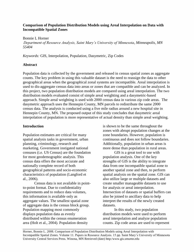
Table 1 displays each zip code with the
number of parcels, area, and population. The
next columns display the five mile/buffer -
number of parcels in the five mile, area per
zip code and what percent of the area lies in
the five mile buffer. The final column
displays the five mile population for each
zip code and total population of the five mile
6
Table 1. Simple areal weighting. Zip codes and five mile buffer area.
ZIP
CODES
NUMBER
OF
PARCELS AREA
POPULATION
PER ZIP
CODE
5 MILE
PARCELS
(NUMBER)
5 MILE
AREA
5 MILE
AREA/AREA
( %)
5 MILE
POPULATION
55316 8477 5523.7 22422 2732 1779.2 0.32 7222
55374 5301 21163.5 9317 873 4623.3 0.22 2035
55327 1612 11302.7 3502 462 5025.9 0.44 1557
55340 2749 22967.3 5836 465 470.3 0.02 120
55369 13047 16100.7 33294 12132 12987.6 0.81 26856
55428 8763 6819.7 29933 20 109.6 0.02 481
55442 4789 5973.6 13196 3 67.9 0.01 150
55446 7029 8713.2 12464 541 794.6 0.09 1137
55311 12811 13793.8 19827 12811 13793.8 1.00 19827
5 MILE TOTAL
POPULATION 59386
buffer – 59386.
Dasymetric interpolation
Dasymetric interpolation is a method of
interpolation that utilizes ancillary data. In
this case, parcels are used as the ancillary
data. The individual parcels are given a
value that corresponds with their description
type.
Single Family/Farm = 4
Condominium and Townhouse = 3
Duplex = 2
Commercial, Industrial, Farmland
and Public Lands = 0
The parcels have an attribute field that lists
the land-use description for each parcel.
This is combined into 4 parcel types – No
Population, Duplex, Condo/Townhouse and
Single Family/Farm. The “No Population”
land use is commercial, industrial and public
lands that do not have population.
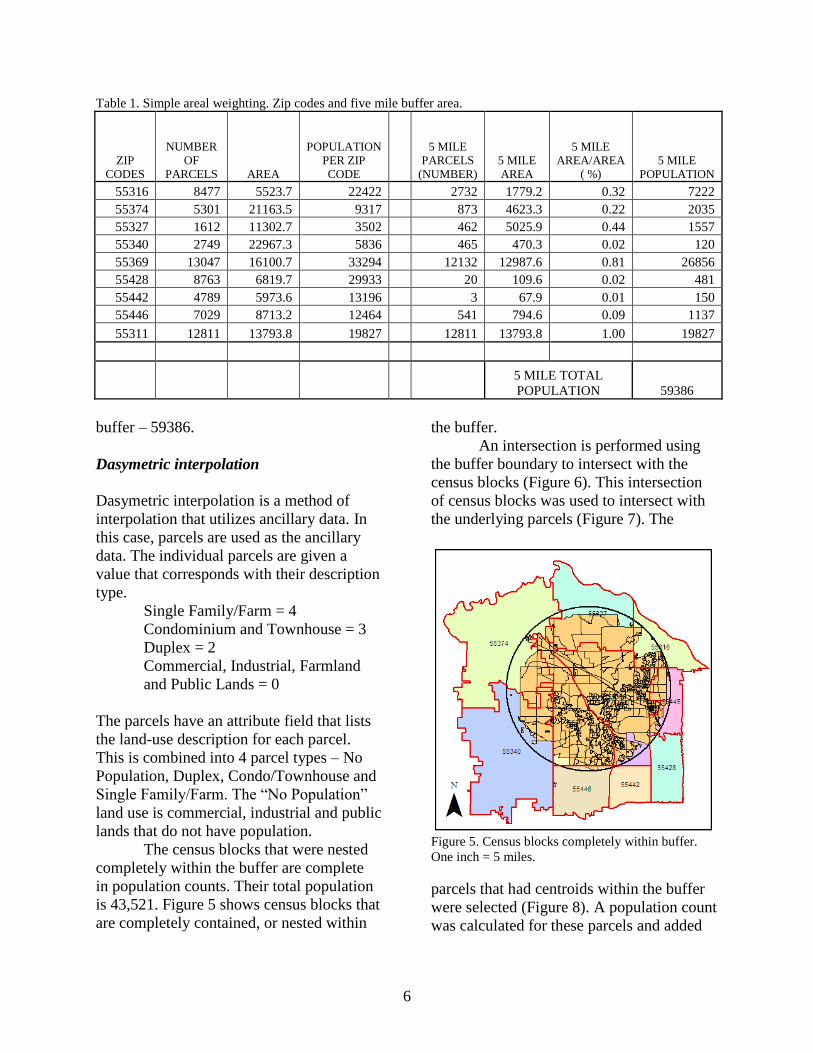
The census blocks that were nested
completely within the buffer are complete
in population counts. Their total population
is 43,521. Figure 5 shows census blocks that
are completely contained, or nested within
the buffer.
An intersection is performed using
the buffer boundary to intersect with the
census blocks (Figure 6). This intersection
of census blocks was used to intersect with
the underlying parcels (Figure 7). The
Figure 5. Census blocks completely within buffer.
One inch = 5 miles.
parcels that had centroids within the buffer
were selected (Figure 8). A population count
was calculated for these parcels and added

7
to the nested census population.
Figure 6. Intersection of Census Blocks and
Boundary. Teal color represents the intersected
blocks. One inch = 5 miles.
Figure 7. Intersection of selected census blocks with
parcels contained within the 5 mile buffer. Purple
represents census block parcels completely within
buffer. One inch = 5 miles.
As with simple areal interpolation, each zip
code has its own population value. To
determine the value to be apportioned to
each parcel in each zip code, a zip code
parcel value for each zip code area was
calculated (Appendix A). The parcels were
divided into the four categories – No
population (NOP), Duplex (DU),
Condo/Townhouse (CT),
Single Family/Farm (SFF) with their
corresponding values as noted here.
NOP = 0 DU = 2
CT = 3 SFF = 4
Each category of values was totaled. The
total population for each zip code was
divided by the total parcel value to calculate
the zip code parcel value that was used to
calculate population in the buffer areas.
Zip Code Population / Parcel value total =
Zip code parcel value.
Figure 8. Parcels within the census blocks
intersection. One inch = 5 miles.
Once a zip code parcel value was calculated
for the parcels in each zip code, that value
was used to determine the population of the
parcels in the census blocks not completely
contained in the buffer.
The next calculation was for the

8
parcels in the census blocks that were not
completely contained in the buffer. The
buffer parcels were again divided into the
four categories. Their values were calculated
and totaled. This total was then multiplied
by the parcel value for each zip code
(Appendix B).
Buffer value total x Parcel value = Buffer
zip code population count.
The counts were then be totaled. This was
the total of the population in the parcels of
the census blocks not completely contained
in the buffer. This count is 6,351 (Appendix
B). When added to the nested census block
population (43,521), the total population of
the buffer is 43,521 + 6,351, or 49,872.
In most dasymetric approaches to
areal interpolation, the counts are divided
into populated versus unpopulated. With the
data already acquired, this calculation can be
performed also. In Table 4, the parcels were
divided into “No Population” versus
“Population.”
No Population = 0
Population = 1
A new parcel value for each zip code was
calculated as shown below.
Zip code population/ Total parcel value =
Parcel value.
This value was used to calculate the buffer
population counts per each zip code and
then was totaled. When this amount was
added to the nested census block totals, the
total population for the buffer was 43,521 +
6,353 = 49,874 (Appendix C).
Results
This study compared two population
distribution models. Simple areal weighting
averages population counts within a zone. In
this study, the zones were zip code areas.
Dasymetric interpolation involved more
analysis, area selection, and calculations.
The difference in the results between the
two distribution models was that with simple
areal weighting, the total population was
estimated to be 59,836 and for dasymetric
interpolation, it was 49,872. When the
categories in the dasymetric interpolation
were changed from 4 categories to 2
categories, the total population is 49,874.
Simple Areal Weighting = 59,836
Dasymetric (4 categories) = 49,872
Dasymetric (2 categories) = 49,874
In Figure 9, all parcels are shown for all zip
codes. In eastern zip codes (55327, 55316,
and 55445), there are areas of no population
in the buffer. The parcels would be
commercial, industrial, farmland or public
lands such as parks, schools, government
buildings. These would skew the results in
the simple areal interpolation. The areas that
have no population would be calculated into
the totals. This is the over-estimation that
Holt (et al., 2004) discusses and is shown in
the representation of population in this study
(Figure 9).
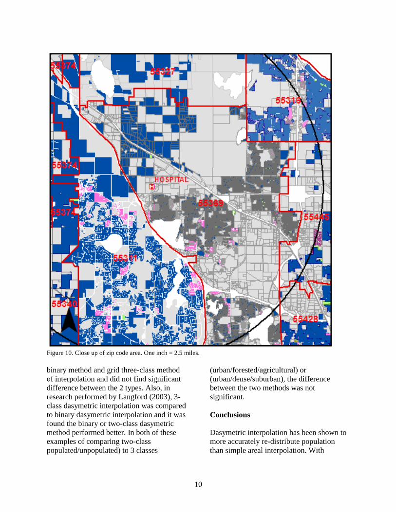
Figure 10 is a “close up” of the zip
code 55369. The light grey areas represent
areas where there is no population. This
shows that the hospital is being built in a
commercial area. What appears to be dark
grey areas are areas of smaller single family
houses. These darker areas have more
population and are visible with dasymetric
interpolation. This difference between areas
of no population and dense population
would not be visible by simple area
weighting.
Though dasymetric interpolation
distributes population more accurately, it is

9
Figure 9. Zip Codes with Parcels and 5 Mile Buffer Boundary. (NOP = No Population; DU = Duplex;
CT = Condominium/Townhouse; SFF = Single Family/Farm). One inch = 2.5 miles.
subjective to what categories are chosen.
The values for single family/farms were
based on the assumption that a single family
is 2 adults and 2 children; therefore, the
value is 4. For condo/townhouse value of 3,
it is based on the reasoning that there would
be more single parents and 2 children or a
young family with 1 child. For duplex, the
value is given for 2 people. As for
commercial, industrial and public lands,
they do not have residents or population.
Apartments were given a value of 4. That
would be very low and not represent the
population of apartments. However, it would
be difficult to know how many units are in
each apartment building without researching
each building.
Even with this subjective choice, the
results did not show much difference
between using 4 categories or 2 categories
for the dasymetric interpolation. This was
consistent with research conducted by
Eicher and Brewer (2001). They performed
dasymetric interpolation using a polygon
10
Figure 10. Close up of zip code area. One inch = 2.5 miles.
binary method and grid three-class method
of interpolation and did not find significant
difference between the 2 types. Also, in
research performed by Langford (2003), 3-
class dasymetric interpolation was compared
to binary dasymetric interpolation and it was
found the binary or two-class dasymetric
method performed better. In both of these
examples of comparing two-class
populated/unpopulated) to 3 classes
(urban/forested/agricultural) or
(urban/dense/suburban), the difference
between the two methods was not
significant.
Conclusions
Dasymetric interpolation has been shown to
more accurately re-distribute population
than simple areal interpolation. With

11
increasingly more powerful computers and
the use of GIS, this analysis is possible.
However, there is not great use of this
technique among the GIS community
(Langford, 2004). Simple areal weighting is
much easier to perform and does not require
any extra ancillary data. The perceived cost
of the ancillary data, added time and
complexity of dasymetric interpolation
hinders its use. There is familiarity with the
simple areal weighting and a lack of
awareness of other possibilities, such as
dasymetric interpolation.
Even though dasymetric mapping
does represent data more closely to actual
population density, it still estimates the
population. This estimation of what most
likely is occurring can be mapped and
shown using dasymetric interpolation
(Poulsen and Kennedy, 2004). With any
population distribution, individuals become
population distributed to patterns or areas.
These patterns or areas are very helpful in
socio-demographic analysis. However, we
are individuals and not estimations.
Acknowledgements
I would like to thank Cliff Moyer for his
insight and technical assistance on this
study, as well as Robert Moulder and
William Brown for the use of the datasets. I
would also like to thank John Ebert and Dr.
Dave McConville of the Resource Analysis
staff at Saint Mary’s University of
Minnesota for his guidance through this
process.
References
Cai, Q. 2006. Estimating Small-Area
Population by Age and Sex Using Spatial
Interpolation and Statistical Inference
Methods. Transitions in GIS, 10, 577-598.
Retrieved January 2008 from EBSCO
database.
Eicher, C. L. and Brewer, C. 2001.
Dasymetric Mapping and Areal
Interpolation: Implementation and
Evaluation. Cartography and Geographic
Information Science, 20, 125-138.
Retrieved February 2008 from EBSCO
database.
Grubesic, T. H. 2006. Zip Codes and
Spatial Analysis: Problems and Prospects.
Socio-Economic Planning Sciences, 42,
129-149. Retrieved January 2008 from
Elsevier Ltd. Database.
Holt, J. B., Lo, C. P., and Holder, T. W.
2004. Dasymetric Estimations of
Population Density and Areal Interpolation
of Census Data. Cartography and
Geographic Information Science, 31, 103-
121.Retrieved January 2008 from SMU
Interlibrary Loan.
Langford, M. 2003. Obtaining Population
Estimates in Non-Census Reporting Zones:
An Evaluation of the 3-class Dasymetric
Method. Computers, Environment and
Urban Systems, 30, 161-180. Retrieved
January 2008 from Science Direct
database.
Langford, M. 2004. Rapid Facilitation of
Dasymetric-Based Population Interpolation
is Means of Raster Pixel Maps. Computers,
Environment and Urban Systems, 31, 19-
32. Retrieved January 2008 from Elsevier
Ltd. database.
Langford, M., Higgs, G., Radcliffe, J., and
White, S. 2006. Urban population
Distribution Models and Service
Accessibility Estimation. Computers,
Environment and Urban Systems, 32, 66-
80. Retrieved January 2008 from Science
Direct database.
Mennis, J. 2003. Generating Surface Models
of Population Using Dasymetric Mapping.
The Professional Geographer, 55, 31-42.
Retrieved February 2008 from Science
Press. 297 pp.

12
Poulsen, E. and Kennedy, L. 2004. Using
Dasymetric Mapping for Spatially
Aggregated Crime Data. Journal of
Quantitative Criminology, 20, 243-262.
Retrieved January 2008 from EBSCO
database.

13
Appendix A. Calculated zip code parcel value.
ZIP
CODE
Commercial
Industry Value = 0
Duplex Value = 2
Condo
Townhouse Value = 3
Single
Family/
Farm value = 4 Totals Population
Zip Code Parcel Value
55311 19827 0.48
parcels 1675 17 3355 7764 12811
values 0 34 10065 31056 41155
55316 22422 0.77
parcels 672 83 937 6785 8477
values 0 186 1874 27140 29200
55327 3502 0.69
parcels 348 0 1 1263 1612
values 0 0 3 5052 5055
55340 5836 0.76
parcels 802 4 123 1820 2749
values 0 2 369 7280 7651
55369 33294 0.78
parcels 1648 75 2671 8653 13047
values 0 150 8013 34612 42775
55374 9317 0.62
parcels 1403 11 420 3462 5296
values 0 22 1260 13848 15130
55428 29933 0.95
parcels 656 110 801 7196 8763
values 0 220 2403 28784 31407
55442 13196 0.80
parcels 314 11 1321 3143 4789
values 0 22 3963 12572 16557
55445 8853 0.72
parcels 633 32 1135 2224 4024
values 0 64 3405 8896 12365
55446 12464 0.58
parcels 1002 6 2735 3286 7029
values 0 12 8205 13144 21361

14
Appendix B. Use parcel value to calculate buffer population.
BUFFER
ZIP
CODE
NOP value = 0
DU value=1
CT value = 3
SFF value = 4
Buffer
Value Total
Zip Code
Parcel Value
Buffer
Population
Total
55311
parcels 124 1 225 0.48
values 0 2 900 902 433
55316
parcels 59 32 675 0.77
values 0 64 2700 2764 2128
55327
parcels 19 1 131 0.69
values 0 2 524 526 363
55340
parcels 32 170 0.76
values 0 680 680 517
55369
parcels 64 3 133 250 0.78
values 0 6 399 1000 1405 1096
55374
parcels 35 2 82 187 0.62
values 0 4 246 748 998 619
55428
parcels 12 7 0.95
values 0 28 28 27
55442
parcels 0.80
values
55445
parcels 70 187 125 0.72
values 0 561 500 1061 764
55446
parcels 175 59 28 124 0.58
values 0 118 84 496 698 405
6351

15
Appendix C. Buffer counts using Population versus No Population.
ZIP
CODE
No
Population value = 0
Populated value=1 Totals
Zip Code Population
Zip Code
Parcel Value
Buffer
No Pop.
Buffer Populated
Buffer
Value Total
Buffer
Pop.
Total
55311 19827
parcels 1675 11136 12811 1.78 124 226
values 0 11136 11136 0 226 226 402
55316 22422
parcels 672 7805 8477 2.87 59 707
values 0 7805 7805 0 707 707 2031
55327 3502
parcels 348 1264 1612 2.77 19 231
values 0 1264 1264 0 132 132 366
55340 5836
parcels 802 1947 2749 3.00 32 170
values 0 1947 1947 0 170 170 510
55369 33294
parcels 1648 11399 13047 2.92 64 383
values 0 11399 11399 0 383 383 1119
55374 9317
parcels 1403 3893 5296 2.39 35 271
values 0 3893 3893 0 271 271 649
55428 29933
parcels 656 8107 8763 3.69 12 7
values 0 8107 8107 0 7 7 26
55442 13196
parcels 314 4475 4789 2.95
values 0 4475 4475
55445 8853 70 312
parcels 633 3391 4024 2.61 0 312 312 815
values 0 3391 3391
55446 12464 175 211
parcels 1002 6027 7029 2.07 0 211 211 436
values 0 6027 6027
6353
Top Related