


Languages
Pages
Legal


Comparison of Analytical, Numerical, and ExperimentalMethods in Deriving Fracture Toughness Properties ofAdhesives Using Bonded Double Lap Joint Specimens
A. R. Setoodeh5Mechanical Engineering Department, Imperial College London,
South Kensington Campus, United Kingdom andMechanical Engineering Department, School of Engineering,Ferdowsi University, Mashhad, Iran
H. Hadavinia10K. Nikbin
Mechanical Engineering Department, Imperial College London,South Kensington Campus, United Kingdom
F. R. BiglariMechanical Engineering Department, Amirkabir University of
15Technology, Tehran, Iran
Stress and fracture analysis of bonded double lap joint (DLJ) specimens have beeninvestigated in this paper. Numerical and analytical methods have been used toobtain shear- and peel-stress distributions in the DLJ. The generalized analyticalsolution for the peel stress was calculated for various forms of the DLJ geometry
20and, by using crack closure integral (CCI) and by means of the J-integralapproach, the analytical strain energy-release rate, G, was calculated. Experi-mental fracture tests have also been conducted to validate the results. The speci-mens were made of steel substrates bonded by an adhesive and loaded undertension. Specimens with cracks on both sides and at either end of the DLJ interface
25were tested to compare the fracture behavior for the two crack positions where ten-sile and compressive peel stresses exist. Tests confirmed that the substrates essen-tially behave elastically. Therefore, a linear elastic solution for the bonded regionof the DLJ was developed. The fracture energy parameter, G, calculated from theelastic experimental compliance for different crack lengths, was compared with
30numerical and analytical calculations using the experimental fracture loads.The stresses from analytical analysis were also compared with those from the finiteelement results. The strain energy-release rate for fracture, Gf, for the adhesive hasbeen shown to have no R-curve resistance, was relatively independent of crack
Received 5 July 2005; in final form 23 January 2005.Address correspondence to K. Nikbin, Mechanical Engineering Department, Imperial
College London, Exhibition Road, London SW7 2AZ, UK. E-mail: [email protected]
The Journal of Adhesion, Vol. 81, No. 5: pp 529–553, 2005Copyright # Taylor & Francis Inc.ISSN: 0021-8464 print=1545-5823 onlineDOI: 10.1080/00218460590944963

length, and compared well with those obtained from numerical and analytical35solutions. However, it was found that fracture energy for the crack starter in the
position where the peel stress was tensile was about 20% lower than where thecrack was positioned at the side, where the peel stress was found to be compressive.
Keywords:Q1
INTRODUCTION
40Adhesive joints are widely used as the principal alternative to conven-tional mechanical fasteners such as screws, rivets, and bolts in indus-try as well as for insulating applications. The basic reasons for thisspecial attention to adhesive joints can be seen in some key points,such as uniform load transfer, removal of any discontinuities in the
45geometry, and reduction of the weight of the structure. These designprocess require that the stress field in the bonded region both in anuncracked and a cracked condition be precisely estimated. In addition,it should be able to predict by the aid of a failure criterion or a fracturemechanics criterion, the strength and durability of bonded joint under
50static or cyclic loading.The objective of the present article is to derive a simplified analyti-
cal solution for a generic DLJ geometry and validate it with numericaland experimental work. Hence, a short review of related previouswork is presented here. There are a number of analytical solutions
55for stress distribution in the lap joint geometry. Different assumptionsand simplifications have been made to reach these solutions.Volkersen [1] made the first attempt to show the elastic behavior ofthe adhesive layer of DLJs, which were subjected to a tensile loading.Goland and Reissner [2] considered cemented single lap joints. Hart-
60Smith [3] developed a more practical modeling for DLJs. He derivedan explicit analytical solution for the static load-carrying capacity ofdouble lap adhesively bonded joints and extended the elastic solutionof Volkersen, which accounted for only imbalance stiffness. Hart-Smith derived both shear- and peel-stress distributions while he made
65some simplifications for uncoupling shear and peel stresses. He alsoderived the solutions for single lap joints [4] and stepped lap joints[5]. Williams [6] produced a general method for the calculation ofenergy-release rates for cracked laminates. Kinloch [7] presented ashear-lag model that took into account the shear deformation of the
70adhesive layer. Hamoush and Ahmad [8] developed a criterion for esti-mating the interface-separation load for adhesive joints of two dissimi-lar materials using a fracture mechanics approach. Bigwood and
2 A. R. Setoodeh et al.

Crocombe [9] developed an elastic analysis for adhesively bonded sin-gle lap joints. Fernlund and Spelt [10] presented an analytical method
75for calculating adhesive-joint fracture parameters using the J-integralmethod. Edde and Verreman [11] derived an analytical solution ofshear and peel stresses for the case of clamped and similar adherendsusing a beam theory as suggested by Goland and Reissner. Chiu andJones [12] presented a numerical study of a thick adherend lap joint
80and a symmetrical DLJ, in which they discussed the effect of varyingadherend and adhesive thicknesses on the stress distribution in thethin adhesive layer. Williams [13] determined the energy-release ratesfor uniform strips in tension and bending. Hadavinia et al. [14] usedCCI and J-integral methods to calculate the strain energy-release rate
85in bonded single lap joints. Lee [15] studied nonlinear behavior oftapered bonded joints and concluded that tapered joints are efficientbecause of the reduction in peel stress at the adherend tips. Her [16]presented an analytical solution for stress analysis of adhesivelybonded lap joints using a simplified one-dimensional model based on
90classical elasticity theory. Pereira and Morais [17] conducted anexperimental study on the strength of adhesively bonded stainlesssteel joints, prepared with epoxy and acrylic adhesives, and measuredMode I critical strain energy-release rate.
MODELING OF DOUBLE LAP JOINT
95In this article, the focus is on the double lap joint (DLJ) as a specialcase. However, the presented method can easily be extended to theanalysis of a single lap joint. The DLJs were made from an epoxyadhesive used to bond the steel substrates. A schematic of a doublelap joint specimen is shown in Figure 1. The outer adherends have
100a Young’s modulus E1, shear modulus G1, Poisson’s ratio n1, and
FIGURE 1 The schematic drawing of a double lap joint (DLJ) geometry andits loading.
Toughness Properties of Adhesives 3

thickness t1, whereas E2, G2, n2, and t2 are Young’s modulus, shearmodulus, Poisson’s ratio, and thickness of inner adherend, respect-ively. The joint overlap length is L and width is w, whereas Ea, Ga,na, and ta are Young’s modulus, shear modulus, Poisson’s ratio, and
105thickness of the adhesive layer, respectively. The double lap jointcan be loaded in tension (compression), F x, and shear, Qx, as well asmoment, Mx, at the substrates’ ends, where the superscript x refersto all external loads applied in a plane normal to x-axis (see Figure 1).
ANALYTICAL SOLUTION
110The classical theory of plates is employed to develop the differentialequations that describe the shear and peel stresses along the bondline.The procedure is general and can be easily used in different situations.Figure 2 shows a free-body diagram of an element of a DLJ in thebonded region. The substrates are considered to behave as linear elas-
115tic cylindrically bent plates. It was assumed that the plate behaves inplane stress condition in the x–z plane and in plane strain condition inthe x–y plane. In this section, the general and simplified solutions ofshear- and peel-stress distribution along the bondline is discussedusing the equilibrium equations of the inner and the outer adherends
120presented in Appendix A.
FIGURE 2 Free-body diagram of a double lap joint element showing thedetail in the bonded region.
4 A. R. Setoodeh et al.

General Solution
The shear strain in the adhesive can be taken as relative displace-ments of the upper (u1) and lower layers (u2) in the x direction, whichare in contact with the substrates. Thus, assuming elastic behavior,
125the shear stress can be written as
sxy ¼Ga
taðu2 � u1Þ ð1Þ
where u is the displacement in the x direction. As presented in Figure 2and under the assumptions made for the state of stress and strain, thecomponent of strains resulting from longitudinal and moment loading
130for the two adherends can be superimposed to obtain the relations
du1
dx¼ n1 F1 þ
6M1
t1
� �;
du2
dx¼ n2 F2 �
6M2
t2
� �ð2Þ
in which subscripts 1 and 2 stand for the outer and the inner adher-ends, respectively, and
ni ¼1� n2iEiti
; i ¼ 1; 2:
135Differentiating Equation (1) and substituting from Equation (2) lead tothe following equation:
dsxydx
¼ Gan2
taF2 � /F1ð Þ � 6
t2M2 þ
/t2t1
M1
� �� �; / ¼ n1
n2: ð3Þ
Two further differentiations from this equation and substitutions ofappropriate equations from Appendix A for moment and longitudinal
140and transverse forces yieldQ2
d2sxydx2
¼ Gan2
ta2þ 4/ð Þsxy �
6
t2Q2 þ
/t2t1
Q1
� �� �ð4Þ
d3sxydx3
�Gan2
ta2þ 4/ð Þdsxy
dxþ 6/
t1ry
� �¼ 0: ð5Þ
Equation (5) is a differential equation in which shear stress, sxy, andpeel stress, ry, are coupled. The shear- and peel-stress distributions
145can be found by deriving another differential equation, and then theshear stress can be uncoupled from the peel stress.
Toughness Properties of Adhesives 5

Hooke’s law for the case of plane stress linear elastic cylindricallybent plates is used to evaluate the relation between the bendingmoment intensity (per unit width) and deformation in the y direction
150[18] as
d2vidx2
¼ �Mi
Di; Di ¼
Eit3i
12ð1� n2i Þ; i ¼ 1; 2: ð6Þ
in which Di is the bending rigidity of the substrates.The elastic peel stress shown in Figure 2 is defined as
ry ¼ �Ea
taðv2 � v1Þ: ð7Þ
155By taking the second to the fourth derivatives of Equation (7) and,after substitution of equilibrium relations from Appendix A, thefollowing differential equations are obtained:
d2rydx2
¼ Ea
taD2M2 � fM1ð Þ; f ¼ D2
D1; ð8Þ
d3rydx3
¼ Ea
taD2Q2 � fQ1 þ
ft12
sxy
� �; ð9Þ
160and
d4rydx4
� Ea
taD1ry þ
t12
dsxydx
� �¼ 0: ð10Þ
It can be seen that, in the fourth-order differential equation, the nor-mal and the shear stresses are again coupled; therefore, stress distri-butions cannot be found directly. The stress field can be found by
165solving Equations (5) and (10) simultaneously to separate the vari-ables. After some manipulations and rearrangements, the followingtwo uncoupled seventh- and sixth-order differential equations interms of a nondimensional parameter, n ¼ x=L, are derived:
d7sxydn7
� k2sd5sxydn5
� 4k4rd3sxydn3
þ 4k2sk4r 1� 3/
2þ 4/
� �dsxy0dn
¼ 0; ð11Þ
d6rydn6
� k2sd4rydn4
� 4k4rd2rydn2
þ 4k2sk4r 1� 3/
2þ 4/
� �ry ¼ 0; ð12Þ
6 A. R. Setoodeh et al.
where
k2s ¼ ð2þ 4/ÞGan2L2
ta; k4r ¼
EaL4
4taD1: ð13Þ
The solution to Equations (11) and (12) is of the form Aern. These dif-ferential equations can be solved in the same way because the auxili-
175ary equation is identical in both cases. The general form of shear andpeel stresses is provided according to the auxiliary Equation (14)under the condition that two roots of it are real (r1,r2) and the thirdroot is imaginary (r3):
R3 � k2sR2 � 4k4rRþ 4k2sk
4r 1� 3/
2þ 4/
� �¼ 0; R ¼ r2: ð14Þ
180Of course, there is a zero root for the shear differential equation. Thegeneral form of stress distributions are
sxy ¼ a1 sinhðr1nÞ þ a2 coshðr1nÞ þ a3 sinhðr2nÞ þ a4 coshðr2nÞþ a5 sinðr3nÞ þ a6 cosðr3nÞ þ a7 ð15Þ
and
ry ¼ b1 sinhðr1nÞ þ b2 coshðr1nÞ þ b3 sinhðr2nÞ þ b4 coshðr2nÞþ b5 sinðr3nÞ þ b6 cosðr3nÞ: ð16Þ
185Boundary conditions were applied to determine the constants of theseequations. These were carried out using MATLAB1 software [19] andby solving the expanded equations numerically or symbolically.
The following boundary conditions were applied for the shear-stressequation:
190. Evaluating Equation (3) at both ends of the overlap joint (n ¼ 0 andn ¼ 1).
. Making the derivative of Equation (5) two more times and substitut-ing for peel-stress differentiation from Equation (8), then evaluatingit at the overlap ends.Q2
195. Making the derivative of Equation (5) three more times and substi-tuting for peel-stress differentiation from Equation (9), then evalu-ating it at the overlap ends.
Toughness Properties of Adhesives 7

. Integrating the second equation in (A2) along the overlap length,which is equal to the net of longitudinal applied force,
Z 1
0
sxydn ¼ 1
2LF2jn¼1 � F2jn¼0
� �¼ c: ð17Þ
A similar procedure can be applied to the peel-stress equation byusing Equations (3) and (8)–(10).
Simplified Solution
The general solution of the stress field was explained in the previous205section. In this section, an alternative, simpler approximate solution
for the peel- and shear-stress distribution, which are easier toimplement, is discussed. Then, the deviation of this approximatesolution relative to the general solution is investigated.
If we assume that the effects of transverse deflection on the shear210distribution is negligible, then the peel stress in Equation (5) can be
ignored and Equation (5) simplifies to
d3sxydn3
� k2sdsxydn
¼ 0 ð18Þ
where ks is the same as defined in Equation (13).The solution of this equation is
sxy ¼ a1 sinhðksnÞ þ a2 coshðksnÞ þ a3: ð19Þ
The following two boundary conditions at either ends of the adhesivelayer and Equation (17) were applied to find the constants a1–a3.
dsxydn
����n¼0;1
¼ Gan2L
taF2 � /F1ð Þ � 6
t2M2 þ
/t2t1
M1
� �� �n¼0;1
¼ a0a1
�: ð20Þ
These constants for dissimilar adherends are as follows:
a1 ¼ a0ks
; a2 ¼ a1 � a0 coshðksÞks sinhðksÞ
; a3 ¼ cþ a0 � a1k2s
: ð21Þ
A simplified solution for the peel-stress distribution was also found byassuming that the shear stress is constant along the overlap length.Then, Equation (10) would be only in terms of the peel stress andthe coupling effect is discarded. In fact, from finite element analysis
225it was found that the shear-stress distribution is nearly uniform andconstant along the overlap length away from the overlap ends. Hence,
8 A. R. Setoodeh et al.

this is a reasonable assumption. The differential equation governingthe peel stress becomesQ3
d4rydn4
� 4k4rry ¼ 0 ð22Þ
230where kr is the same as defined in Equation (13). Equation (22) has thefollowing solution:
ry ¼ b1 sinðkrnÞ sinhðkrnÞ þ b2 cosðkrnÞ coshðkrnÞþ b3 sinðkrnÞ coshðkrnÞ þ b4 cosðkrnÞ sinhðkrnÞ: ð23Þ
Evaluating Equations (8) and (9) at either ends of the overlap producesfour equations to find the constants b1–b4. These equations were
235solved simultaneously by the symbolic toolbox of MATLAB and theresults are presented in Appendix B.
CRACK CLOSURE INTEGRAL (CCI)
The stress field is now known according to the equations derived in theprevious section. The fracture mechanics parameters can be easily
240estimated if the energy-release rate, G, can be expressed in terms ofstress values at the crack tip. Consider the strain energy-release rate(SERR) when a crack grows an amount Da; that is, the crack advancesfrom state (a) to state (b) as shown in Figure 3. In this situation, the
FIGURE 3 Schematic view of crack growth from state (a) at crack incrementa to state (b) with crack increment aþDa.
Toughness Properties of Adhesives 9
shear and peel stresses relax from some value to zero over the crack245advance increment Da, while the crack tip moves from A to A0 by Du
and Dv in the x and y directions, respectively. The former change indisplacement is caused by the normal stress component, which contri-butes to Mode I fracture, whereas the latter one is due to the shear-stress component and contributes to Mode II fracture. Alternatively,
250the result would be the same if we consider the work required to closethe crack an amount Da. The energy release rate per unit thicknessover this crack growth can be written as
GDa ¼ 1
2
Z Da
0
sxyDuþ ryDv
dx1: ð24Þ
The SERR can be computed from Equation (24) by dividing both sides255by Da and letting Da ! 0 (note that stresses are maximum at either
ends of overlap according to the derived equations). The variation indisplacement is the relative displacement of the two adherends (seeFigure 3); therefore, Equation (24) can be rearranged as
G ¼ 0:5ss ðu2 � u1Þ þ 0:5rr ðv2 � v1Þ ð25Þ
260where ss and rr are shear and peel stresses at the crack tip. Substitutingfor displacements from Equations (1) and (7) yields
GI ¼ta2Ea
rr2; GII ¼ta2Ga
ss2; ð26Þ
and the total strain energy-release rate is G ¼ GI þGII.For linear elastic materials, a simplified relationship between the
265energy-release rate, G, and stress-intensity factor, K, can be presentedas
G ¼ ð1� n2aÞEa
K2I þ K2
II
: ð27Þ
For the DLJ specimens, it was determined that the failure mechanismwas mixed mode. For the present, therefore, no attempt is made to dif-
270ferentiate between the two modes but rather to determine the totalfracture energy-release rate, G, to compare it with the experimentalvalues.
J-INTEGRAL METHOD
In this section, the J-integral approach is implemented to calculate275fracture parameters and, unlike the CCI method, it can be applied
to nonlinear elastic behavior. This integral can be written for the
10 A. R. Setoodeh et al.

problem under consideration as
J ¼IC
WðeÞn1 � rijnj@Ui
@x
� �ds ð28Þ
where C is a closed contour that encloses the crack tip and part of the280adhesive layer over the bonded lap, W is the strain energy per unit
volume, nj is the direction cosine of the outward unit normal vectorto C, and U(u,v) is the displacement vector along the contour. Thisequation can be expanded as
J ¼IC
Z e
0
rijdeij
� �n1 � rxn1 þ sxyn2
@u@x
� sxyn1 þ ryn2
@v@x
� �ds:
ð29Þ
285Figure 4 shows the contour along which the line integral was calcu-lated. By definition, there is no traction on the crack faces and alson1 ¼ 0 along contour parts 2 and 3; thus, the line integral is zero onthese parts. Along divisions 1, 4, and 6, n2 ¼ 0 and only nonzero stresscomponents contribute to the strain energy density. For contour parts
2905 and 7, n1 ¼ 0. Therefore, the nonzero components of the J integralwould be
J1;4 ¼Z ta=2
�ta=2
Z ey
0
rydey
x¼0
� �dy on C1;4; ð30Þ
J5 ¼Z aþDa
0
sxy@u
@xþ ry
@v
@x
� �dx on C5; ð31Þ
J6 ¼Z ta=2
�ta=2
Z e
0
rydey þ 2sxydexy
x¼aþDa
� �dy on C6; ð32Þ
FIGURE 4 Description of the J-integral contour around the crack in theadhesive layer region.
Toughness Properties of Adhesives 11

295and
J7 ¼ �Z aþDa
0
sxy@u
@xþ ry
@v
@x
� �dx on C7: ð33Þ
Equations (30) and (32) should be integrated over the adhesive thick-ness. Because the adhesive layer is thin, it is reasonable to assumethat the variation in stresses in the normal direction across the
300adhesive layer is negligible. Hence, the J integral on divisions 1, 4,and 6 can be ignored. Therefore, the J integral results from addingEquations (31) and (33), noting that displacements on division 7 aredue to adherend 1 and displacements along division 5 belong to adher-end 2:
J ¼Z aþDa
0
sxy@u2
@x� @u1
@x
� �þ ry
@v2@x
� @v1@x
� �� �dx: ð34Þ
Differentiating Equations (1) and (7) and then substituting fordisplacement differences leads to
J ¼Z aþDa
0
taGa
sxydsxydx
þ taEa
rydrydx
� �dx: ð35Þ
Noting that when the crack grows, stresses are relaxed, and because310the adhesive layer is thin, the stress field at the region between
x ¼ 0 and x ¼ a is negligible. Thus, the lower bound of the integralcan be replaced by a. Now, if Da ! 0, the shear and peel stresses havevalues at the crack tip of ss and rr, respectively, and then
J ¼ ta2Ga
ss2 þ ta2Ea
rr2: ð36Þ
315The J-integral approach resulted in the same relationship as wasachieved from the CCI in Equation (26).
NUMERICAL SOLUTION
The finite element (FE) model of the DLJ was considered as consistingof two isotropic, homogeneous and linear–elastic materials joined
320together along interfaces, as shown in Figure 1. Because of symmetry,only one half of the DLJ was modeled under a plane strain assump-tion. It should be noted that the analytical model described cannot dis-tinguish between crack growth cohesively through the center of theadhesive layer and crack growth at the adhesive=substrate interfaces.
325However, the FE approach can obviously model either a cohesive or an
12 A. R. Setoodeh et al.

interfacial crack. The analysis was undertaken using ABAQUS soft-ware [20].
The J-integral method was used to calculate values of G as a func-tion of the crack length, a. Smelser and Gurtin [21] have shown that
330the J integral for a nonhomogeneous solid composed of dissimilarmaterials is the same as the analogous result for a single-phasematerial. Thus, for an interfacial crack problem, the line integralhas the same form as the well-known J-integral for monolithic solids,provided the surfaces are free from traction and the interface is a
335straight line.For a quasi-static crack advance, two methods are typically used for
calculating the J integral in a two-dimensional analysis. One methodis based on a line-integral expression and the other method uses thedivergence theorem, where the contour integral can be expanded into
340an area integral over a finite domain that surrounds the crack tip. InFEA, coordinates and displacements refer to nodal points and stressesand strain refers to the Gaussian integration point.Q2 Hence, it is moreconvenient to evaluate the contour integral using the domain integraland this method is used in ABAQUS. The number of different evalua-
345tions of J possible is the number of such rings of elements.For small scale and contained yielding, a path-independent integral
can be computed outside the plastic zone. This means that the J con-tour has to be large enough to surround the plastic zone and passthrough the elastic region only. However, in a blunting crack case, sig-
350nificant stress redistribution occurs at the crack tip and the pathdependence increases strongly. Also, as the stress singularity at theblunting crack tip vanishes under the assumption of finite strainsand incremental plasticity, J will not have a finite value any more.This is because the work dissipated by plastic deformation should
355always be positive and the calculated J values have to increase mono-tically with the size of the domain, except for the contour that touchesthe domain boundaries. For these cases, the highest calculated J valuewith increasing domain size in the far-field remote from the crack tipis always the closest to the real far-field J. Accurate estimates of the
360contour integral are usually determined even with quite coarsemeshes.
In the elastic analysis, the cracks were assumed to be sharp, andthe crack faces were assumed to lie on top of one another in the unde-formed configuration. These types of cracks are normally analyzed
365under small-strain assumptions, as the strain field is singular at thecrack tip and this singular zone is localized. The variations in the esti-mates of the J integral from domain rings, excluding the crack tipitself, were very small. The present FE modeling was performed
Toughness Properties of Adhesives 13

assuming linear–elastic behavior. Material properties used in the FEA370are summarized in Table 1. In the present work, four-noded isopara-
metric elements were used for the whole domain. A typical modelof the joint was composed of 10,000 elements and 10,431 nodes (seeFigure 5). A range of crack lengths were used in the model and thecrack was positioned at the point A or D of the geometry as shown
375in Figures 1 and 5. The results for the stress analysis are presentedin a later section. Also, the displacements measured between positionsA and D in Figure 5 are used to derive the compliance for differentcrack lengths to compare with the experimental values measured atthe same positions as described in the next section.
380EXPERIMENTS
The substrates used throughout the present article were preparedfrom a 316 stainless steel and were bonded by using a hot-curing
TABLE 1 Properties of Double Lap Joint Specimens
Adherend 1–steel Adherend 2–steel Adhesive
Young’s modulus, E (GPa) 207 207 4Poisson’s ratio, n 0.3 0.3 0.38Thickness, t (mm) 6 12 1Yield stress (MPa) 350 350 35
FIGURE 5 Finite element mesh for the half section of the double lap joint(DLJ) specimen.
14 A. R. Setoodeh et al.

toughened-epoxy adhesive ESP110 (Permabond Eastleigh, UK). Priorto bonding, the steel substrates were pretreated using a grit-blast and
385degrease (GBD) treatment. For these joints, the substrates were firstwashed with water to remove any gross contamination, after whichthey were degreased with acetone. The substrates were lightly grit-blasted with alumina grit and any grit was removed with compressedair. They were then cleaned with acetone, washed in cold tap water,
390and dried prior to being bonded.The double lap joint specimens (shown schematically in Figure 1)
were made from two outer 6-mm stainless steel plates and an inner12-mm stainless steel plate with the width of w ¼ 20mm. After thesteel plates were pretreated, they were bonded with an overlap length
395of L ¼ 20mm. The bonded plates were held together using clips whilethey were cured for 60min at 180�C. The specimens were then allowedto cool in the oven, during which procedure naturally occurring spewfillets of adhesive formed at the ends of the overlap. Different sizesof precracks were inserted at point A and point D and the symmetrical
400location is shown in Figure 1 of both bondlines where a thin sheet ofPTFE had been inserted prior to curing.
The specimens were tested-under monotonic tensile-loading con-ditions. The joints were loaded using a constant displacement rate of1mm=min in a ‘‘dry’’ environment at room temperature and failed
405under tensile applied loads, P, to different failure loads of Pf. The fail-ure loads of the double lap joint with different precrack lengths forposition A and D are summarized in Table 2. The displacement wasmeasured both with an extensometer placed between positions
TABLE 2 Compliance and Fracture Energy of DLJ Specimen Derived fromExperimental, Analytical, and Numerical Calculations for Different CrackLength
Crack at position D Crack at position A
Experiments Analytical FEA Experiments Analytical FEA
Crack
length (mm)
Failure load,
Pf (kN)
Gf
(J=m2)
Gf
(J=m2)
Gf
(J=m2)
Failure load,
Pf (kN)
Gf
(J=m2)
Gf
(J=m2)
Gf
(J=m2)
0 33.9 — — — 36.5 — — —
2 28.2 662 823 750 34.2 600 983 870
4 24.6 688 944 732 32 841 1143 930
6 20.8 694 741 691 27.6 937 954 920
8 17.2 660 762 640 23 915 942 855
10 15.1 689 730 683 17.1 680 748 660
12 12.2 591 699 626 14.2 603 745 670
Toughness Properties of Adhesives 15
A and D as shown in Figure 5 and remotely between the grips using410the testing machine displacement recorder. The local displacement
measurements between A and D were used to derive the compliancefor different crack lengths and crack positions. An example of the loaddisplacement measured locally with an extensometer and globallyusing the machine displacement for a precrack length of 8mm are
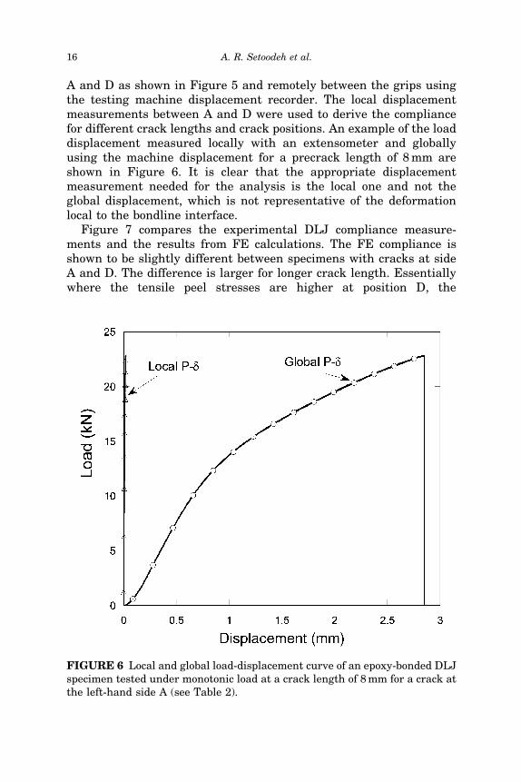
415shown in Figure 6. It is clear that the appropriate displacementmeasurement needed for the analysis is the local one and not theglobal displacement, which is not representative of the deformationlocal to the bondline interface.
Figure 7 compares the experimental DLJ compliance measure-420ments and the results from FE calculations. The FE compliance is
shown to be slightly different between specimens with cracks at sideA and D. The difference is larger for longer crack length. Essentiallywhere the tensile peel stresses are higher at position D, the
FIGURE 6 Local and global load-displacement curve of an epoxy-bonded DLJspecimen tested under monotonic load at a crack length of 8mm for a crack atthe left-hand side A (see Table 2).
16 A. R. Setoodeh et al.

compliance tends to be larger when compared with cracks at position425A. The agreement is reasonable, with the experimental results falling
slightly lower than the FE calculations, hence making the FE com-pliance a conservative estimate. Using the FE results, the complianceof the DLJ can be described as a function of crack length by
C ¼ d=p ¼ f ðaÞ ð37Þ430where p ¼ P=2w and
f ðaÞ ¼ 1:24� 10�8a3 þ 1:4� 10�7a2 þ 9:15� 10�7aþ 5� 10�5 ðSide AÞ;f ðaÞ ¼ 2:15� 10�8a3 þ 5:1� 10�8a2 þ 2:2� 10�6aþ 5� 10�5 ðSide DÞ:
ð38ÞIn these, the dimension of p is in N=mm and d is in mm. The experi-mental fracture energy was then calculated from the measured failureload per unit width per arm, pf ¼ Pf =2w, by
G ¼p2f
2
dC
dað39Þ
FIGURE 7 Comparison of DLJ compliance measured from experiments andobtained from FEA.
Toughness Properties of Adhesives 17

where
dC
da¼ 3:72� 10�8a2 þ 2:8� 10�7aþ 9:15� 10�7 ðSide AÞ;
dC
da¼ 6:45� 10�8a2 þ 1:02� 10�7aþ 2:2� 10�6 ðSide DÞ:
ð40Þ
The results of experimental compliance and fracture energy are pre-sented in Table 2. The locus of failure was found to be a mixture of
440interfacial (visually) and cohesive fracture for all joints.
COMPARISON OF ANALYTICAL AND NUMERICAL RESULTS
Several examples were solved to show the accuracy of the analyticalsolution in comparison with the numerical analysis. Both stress distri-butions and fracture parameters were obtained. Comparisons with
445experimental data were made in some cases. The importance of shear-and peel-stress components can be judged from the results and deci-sions can be made whether to use the general solution or the simplifiedone. The shear and peel stresses were normalized by multiplying themby the factor ðt2=Fx
2Þ. A sample of a contour plot of shear- and peel-450stress distribution in DLJ from FEA is shown in Figure 8 for crack
positions A and D.In the first example, a DLJ without any crack was considered. The
joint was under tensile loading of Fx2 ¼ 2Fx
1 ¼ 600N=mm. Figure 9compares the shear-stress distribution along the interface of adhesive
455and adherend 2 obtained from numerical and analytical solutions.Both general and simplified solutions are shown. The analytical sol-ution shows good agreement with finite element results and thegeneral solution generally gives a more accurate representation. Somediscrepancies can be seen at the overlap ends. In fact, these spots
460act like singular points and the finite element method tries to modelthe zero stress state at traction-free end surfaces. The differencebetween stress distribution from analytical and FEA solutions alongthe overlap and away from its ends is negligible. In Figure 10Q4 peel-stress distribution resulting from simplified analytical and FEA solu-
465tions along the interface CD in an uncracked DLJ are compared.Again, the analytical solution agrees quite well with the FEA results.
Figure 11 shows the effect of the crack length on the shear-stressdistribution obtained from the general solution and the FEA. Two dif-ferent crack lengths of 2mm and 5mm at position A were considered
470on one side of the bondline (as shown in Figures 1 and 5) and the stressdistribution was plotted along the cracked side of the adhesive.
18 A. R. Setoodeh et al.

FIGURE 8 Distribution of peel stress and shear stress along the bonded partof DLJ at a crack length of 4mm with the crack placed either at side D or atside A.
Toughness Properties of Adhesives 19

In Figure 12, a similar comparison between peel stress computed fromthe simplified solution and the FEA for the same crack lengths ismade. In all cases, the agreement between analytical solution and
475FEA was generally acceptable except in the vicinity of the crack tip.
COMPARISON WITH EXPERIMENTAL RESULTS
The peel-stress contours at the crack tips in Figures 8c and d suggestthat the specimen is subjected to mixed-mode loading, although ModeI seems to be dominant. It is also observed that the tensile peel stres-
480ses at position D cause crack opening, while the compressive peelstress at position A causes crack closure. This affects, the fractureenergy depending on the crack position.
For each experimental case shown in Table 2, the specific values ofthe strain energy-release rate, Gf, from the experiments, FEA J inte-
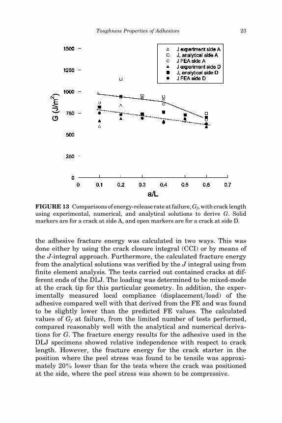
485grals, and the analytical calculations were derived and compared.Figure 13 compares the strain energy-release rates with the fracturecomputed for each test case versus the normalized crack length, a=L.The experimental, analytical, and numerical solutions for Gf show avery good overall agreement. The increased discrepancy at the shorter
FIGURE 9 Distribution of shear stress along the interface CD betweenadhesive and adherend 2 (uncracked DLJ).
20 A. R. Setoodeh et al.
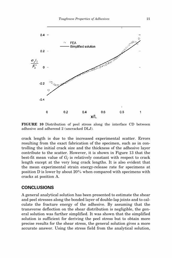
490crack length is due to the increased experimental scatter. Errorsresulting from the exact fabrication of the specimen, such as in con-trolling the initial crack size and the thickness of the adhesive layercontribute to the scatter. However, it is shown in Figure 13 that thebest-fit mean value of Gf is relatively constant with respect to crack
495length except at the very long crack lengths. It is also evident thatthe mean experimental strain energy-release rate for specimens atposition D is lower by about 20% when compared with specimens withcracks at position A.
CONCLUSIONS
500A general analytical solution has been presented to estimate the shearand peel stresses along the bonded layer of double-lap joints and to cal-culate the fracture energy of the adhesive. By assuming that thetransverse deflection on the shear distribution is negligible, the gen-eral solution was further simplified. It was shown that the simplified
505solution is sufficient for deriving the peel stress but to obtain moreprecise results for the shear stress, the general solution gives a moreaccurate answer. Using the stress field from the analytical solution,
FIGURE 10 Distribution of peel stress along the interface CD betweenadhesive and adherend 2 (uncracked DLJ).
Toughness Properties of Adhesives 21

FIGURE 11 Shear-stress profile at two different crack lengths at point Calong the bondline of adherend 2.
FIGURE 12 Peel-stress profile at two different crack lengths at point C alongthe bondline of adherend 1.
22 A. R. Setoodeh et al.
the adhesive fracture energy was calculated in two ways. This wasdone either by using the crack closure integral (CCI) or by means of
510the J-integral approach. Furthermore, the calculated fracture energyfrom the analytical solutions was verified by the J integral using fromfinite element analysis. The tests carried out contained cracks at dif-ferent ends of the DLJ. The loading was determined to be mixed-modeat the crack tip for this particular geometry. In addition, the exper-
515imentally measured local compliance (displacement=load) of theadhesive compared well with that derived from the FE and was foundto be slightly lower than the predicted FE values. The calculatedvalues of Gf at failure, from the limited number of tests performed,compared reasonably well with the analytical and numerical deriva-
520tions for G. The fracture energy results for the adhesive used in theDLJ specimens showed relative independence with respect to cracklength. However, the fracture energy for the crack starter in theposition where the peel stress was found to be tensile was approxi-mately 20% lower than for the tests where the crack was positioned
525at the side, where the peel stress was shown to be compressive.
FIGURE 13 Comparisonsof energy-release rateat failure,Gf,withcrack lengthusing experimental, numerical, and analytical solutions to derive G. Solidmarkers are for a crack at side A, and open markers are for a crack at side D.
Toughness Properties of Adhesives 23
ACKNOWLEDGMENT
The authors thank A. Nyilas of Forschungszentrum Karlsruhe,Germany, for his help and advice.
REFERENCES
530[1] Volkersen, O., Luftfahrtforschung 15, 41–47 (1938).[2] Goland, M. and Reissner, E., J. Appl. Mech. 11, A17–A24 (1944).[3] Hart-Smith, L. J., Technical Report NASA CR 112235, Douglas Aircraft Company
(1973).Q5
[4] Hart-Smith, L. J., Technical Report NASA CR 112236, Douglas Aircraft Company,535(1973).
[5] Hart-Smith, L. J., Technical Report NASA CR 112237, Douglas Aircraft Company,(1973).
[6] Williams, J. G., Int. J. Fract. 36, 101–119 (1988).[7] Kinloch, A. J., Adhesion and Adhesives: Science and Technology (Chapman and
540Hall, London, 1987).[8] Hamoush, S. A. and Ahmad, S. H., Int. J. Adhes. Adhes. 9, 171–178 (1989).[9] Bigwood, D. A. and Crocombe, A. D., Int. J. Adhes. Adhes. 9, 229–242 (1989).[10] Fernlund, G., Spelt, J. K., Engng. Fract. Mech. 40, 119–132 (1991).[11] Edde, F. and Verreman, Y., Int. J. Adhes. Adhes. 12, 43–48 (1992).
545[12] Chiu, W. K. and Jones, R., Int. J. Adhes. Adhes. 12, 219–225 (1992).[13] Williams, J. G., J. Strain Analysis 28, 237–246 (1993).[14] Hadavinia, H., Kinloch, A. J., Little, M. S. G., and Taylor, A. C., Int. J. Adhes.
Adhes. 23(6), 463–471 (2003).[15] Lee, K. J., Comput. Struct. 56, 637–643 (1995).
550[16] Her, S. C., J. Comp. Struct. 47, 673–678 (1999).[17] Pereira, A. B. and Morais, A. B. Int. J. Adhes. Adhes. 23, 315–322 (2003).[18] Dym, C. L. and Shames, I. H., Solid Mechanics: A Variational Approach (McGraw-
Hill, New York, 1973).[19] Hunt, B., Lipsman, R., and Rosenberg, G., A guide to MATLAB (Cambridge Univer-
555sity press, Cambridge, 2001).[20] Hibbitt, Karlsson & Sorensen, Inc., ABAQUS=CAE version 6.2 (2001).Q6
[21] Smelser, R. E. and Gurtin, M. E., Int. J. Fract. 13, 382–384 (1977).
APPENDIX A
The force and moment equilibrium equations for a differential560element, dx, within the joint can be written as follows (see Figure 2):
dQ1
dx¼ �ry
dF1
dx¼ �sxy
dM1
dx¼ Q1 �
t12sxy;
8>>>>>><>>>>>>:
ðA1Þ
24 A. R. Setoodeh et al.

dQ2
dx¼ 0
dF2
dx¼ 2sxy
dM2
dx¼ Q2
8>>>>>><>>>>>>:
ðA2Þ
where subscripts 1 and 2 stand for the outer and the inner adherends,respectively. The equations were derived for a unit width in the z
565direction.
APPENDIX B
The right-hand sides of Equations (8) and (9) were evaluated at eitherends of the bonded region to calculate the constants of Equation (23) as
EfL2
2taD2k2rðM2 � fM1Þ ¼
T1 at n ¼ 0T2 at n ¼ 1;
�ðB1Þ
Q2 � fQ1 þft12
sxy
� �L3
2k3r¼ T3 at n ¼ 0
T4 at n ¼ 1;
�ðB2Þ
then the second and third differentiations of Equation (23) were alsoevaluated at these geometrical points to develop a relation betweenthe b1–b4 coefficients and Equations (B1) and (B2). The solution of thissystem of equations would be as follows:
b1 ¼ T1=s4;
b2 ¼ fT1ðs41 þ 4s21s2s3 � 1Þ þ 2T2½s1ðs3 � s2Þ � s31ðs3 þ s2Þ�þ 4T3s
21s
22 þ 2T4s2ðs31 � s1Þg=s4;
b3 ¼ f�T1½ðs21 � 1Þ2 þ 4s21s22� þ 4T2s2ðs31 � s1Þ
þ T3ð�s41 þ 4s21s2s3 þ 1Þþ 2T4½s31ðs3 � s2Þ � s1ðs3 þ s2Þ�g=s4;
b4 ¼ fT1ðs41 þ 4s21s2s3 � 1Þ þ 2T2½s1ðs3 � s2Þ � s31ðs3 þ s2Þ�þ T3ðs41 � 2s21 þ 1Þ þ 2T4s2ðs31 � s1Þg=s4;
ðB3Þ
in which
s1 ¼ expðkrÞ; s2 ¼ sinðkrÞ; s3 ¼ cosðkrÞ ðB4Þ
s4 ¼ 4s21s22 � ðs21 � 1Þ2: ðB5Þ
Toughness Properties of Adhesives 25
Top Related