


Languages
Pages
Legal

CODATA recommended values of the fundamental physical
constants: 2010*
Peter J. Mohr,† Barry N. Taylor,‡ and David B. Newell§
National Institute of Standards and Technology, Gaithersburg, Maryland 20899-8420, USA
(published 13 November 2012)
This paper gives the 2010 self-consistent set of values of the basic constants and conversion factors
of physics and chemistry recommended by the Committee on Data for Science and Technology
(CODATA) for international use. The 2010 adjustment takes into account the data considered
in the 2006 adjustment as well as the data that became available from 1 January 2007, after the
closing date of that adjustment, until 31 December 2010, the closing date of the new adjustment.
Further, it describes in detail the adjustment of the values of the constants, including the selection of
the final set of input data based on the results of least-squares analyses. The 2010 set replaces the
previously recommended 2006 CODATA set and may also be found on the World Wide Web at
physics.nist.gov/constants.
DOI: 10.1103/RevModPhys.84.1527 PACS numbers: 06.20.Jr, 12.20.�m
CONTENTS
I. Introduction 1528
A. Background 1528
B. Brief overview of CODATA 2010 adjustment 1529
1. Fine-structure constant � 1529
2. Planck constant h 1529
3. Molar gas constant R 1530
4. Newtonian constant of gravitation G 1530
5. Rydberg constant R1 and proton radius rp 1530
C. Outline of the paper 1530
II. Special Quantities and Units 1530
III. Relative Atomic Masses 1531
A. Relative atomic masses of atoms 1531
B. Relative atomic masses of ions and nuclei 1532
C. Relative atomic masses of the proton, triton,
and helion 1532
D. Cyclotron resonance measurement of the
electron relative atomic mass 1533
IV. Atomic Transition Frequencies 1533
A. Hydrogen and deuterium transition frequencies,
the Rydberg constant R1, and the proton and
deuteron charge radii rp, rd 1533
1. Theory of hydrogen and deuterium
energy levels 1534
a. Dirac eigenvalue 1534
b. Relativistic recoil 1534
c. Nuclear polarizability 1535
d. Self energy 1535
e. Vacuum polarization 1536
f. Two-photon corrections 1536
g. Three-photon corrections 1539
h. Finite nuclear size 1539
i. Nuclear-size correction to self energy and
vacuum polarization 1539
j. Radiative-recoil corrections 1539
k. Nucleus self energy 1540
l. Total energy and uncertainty 1540
m. Transition frequencies between levels
with n ¼ 2 and the fine-structure constant � 1540
n. Isotope shift and the deuteron-proton
radius difference 1540
2. Experiments on hydrogen and deuterium 1541
3. Nuclear radii 1542
a. Electron scattering 1542
b. Muonic hydrogen 1543
B. Antiprotonic helium transition frequencies
and ArðeÞ 1543
1. Theory relevant to antiprotonic helium 1544
2. Experiments on antiprotonic helium 1544
3. Inferred value of ArðeÞ from antiprotonic
helium 1545
C. Hyperfine structure and fine structure 1545
V. Magnetic-Moment Anomalies and g-Factors 1546
A. Electron magnetic-moment anomaly aeand the fine-structure constant � 1546
1. Theory of ae 1546
2. Measurements of ae 1547
a. University of Washington 1547
*This report was prepared by the authors under the auspices of the
CODATATaskGroup on Fundamental Constants. Themembers of the
task group are F. Cabiati, Istituto Nazionale di Ricerca Metrologica,
Italy; J. Fischer, Physikalisch-Technische Bundesanstalt, Germany;
J. Flowers, National Physical Laboratory, United Kingdom; K. Fujii,
National Metrology Institute of Japan, Japan; S.G. Karshenboim,
Pulkovo Observatory, Russian Federation; P. J. Mohr, National
Institute of Standards and Technology, United States of America;
D.B. Newell, National Institute of Standards and Technology,
United States of America; F. Nez, Laboratoire Kastler-Brossel,
France; K. Pachucki, University of Warsaw, Poland; T. J. Quinn,
Bureau international des poids et mesures; B.N. Taylor, National
Institute of Standards and Technology, United States of America;
B.M. Wood, National Research Council, Canada; and Z. Zhang,
National Institute of Metrology, People’s Republic of China.†[email protected]‡[email protected]§[email protected]
REVIEWS OF MODERN PHYSICS, VOLUME 84, OCTOBER–DECEMBER 2012
0034-6861=2012=84(4)=1527(79) 1527 Published by the American Physical Society
b. Harvard University 1547
3. Values of � inferred from ae 1548
B. Muon magnetic-moment anomaly a� 1548
1. Theory of a� 1548
2. Measurement of a�: Brookhaven 1549
C. Bound-electron g-factor in 12C5þ
and in 16O7þ and ArðeÞ 1549
1. Theory of the bound electron g-factor 1550
2. Measurements of geð12C5þÞ and geð16O7þÞ 1552
VI. Magnetic-moment Ratios and
the Muon-electron Mass Ratio 1553
A. Magnetic-moment ratios 1553
1. Theoretical ratios of atomic bound-particle
to free-particle g-factors 1553
2. Bound helion to free helion magnetic-moment
ratio �0h=�h 1554
3. Ratio measurements 1554
B. Muonium transition frequencies, the
muon-proton magnetic-moment ratio ��=�p,
and muon-electron mass ratio m�=me 1554
1. Theory of the muonium ground-state
hyperfine splitting 1555
2. Measurements of muonium transition
frequencies and values of ��=�p and m�=me 1556
VII. Quotient of Planck Constant
and Particle Mass h=mðXÞ and � 1557
A. Quotient h=mð133CsÞ 1557
B. Quotient h=mð87RbÞ 1557
C. Other data 1558
VIII. Electrical Measurements 1558
A. Types of electrical quantities 1558
B. Electrical data 1559
1. K2JRK and h: NPL watt balance 1559
2. K2JRK and h: METAS watt balance 1560
3. Inferred value of KJ 1560
C. Josephson and quantum-Hall-effect relations 1560
IX. Measurements Involving Silicon Crystals 1561
A. Measurements of d220 Xð Þ of natural silicon 1561
B. d220 difference measurements of natural
silicon crystals 1562
C. Gamma-ray determination of the neutron
relative atomic mass ArðnÞ 1562
D. Historic x-ray units 1562
E. Other data involving natural silicon crystals 1563
F. Determination of NA with enriched silicon 1563
X. Thermal Physical Quantities 1564
A. Acoustic gas thermometry 1564
1. NPL 1979 and NIST 1988 values of R 1564
2. LNE 2009 and 2011 values of R 1565
3. NPL 2010 value of R 1565
4. INRIM 2010 value of R 1565
B. Boltzmann constant k and quotient k=h 1566
1. NIST 2007 value of k 1566
2. NIST 2011 value of k=h 1566
C. Other data 1567
D. Stefan-Boltzmann constant � 1567
XI. Newtonian Constant of Gravitation G 1567
A. Updated values 1568
1. National Institute of Standards and
Technology and University of Virginia 1568
2. Los Alamos National Laboratory 1568
B. New values 1568
1. Huazhong University of Science and
Technology 1568
2. JILA 1569
XII. Electroweak Quantities 1569
XIII. Analysis of Data 1569
A. Comparison of data through inferred values
of �, h, k, and ArðeÞ 1569
B. Multivariate analysis of data 1571
1. Data related to the Newtonian constant
of gravitation G 1575
2. Data related to all other constants 1577
3. Test of the Josephson and
quantum-Hall-effect relations 1583
XIV. The 2010 CODATA Recommended Values 1586
A. Calculational details 1586
B. Tables of values 1594
XV. Summary and Conclusion 1595
A. Comparison of 2010 and 2006 CODATA
recommended values 1595
B. Some implications of the 2010 CODATA
recommended values and adjustment for
metrology and physics 1595
C. Suggestions for future work 1597
List of Symbols and Abbreviations 1597
Acknowledgments 1599
References 1599
I. INTRODUCTION
A. Background
This article reports work carried out under the auspices ofthe Committee on Data for Science and Technology(CODATA) Task Group on Fundamental Constants.1 It de-scribes in detail the CODATA 2010 least-squares adjustmentof the values of the constants, for which the closing date fornew data was 31 December 2010. Equally important, it givesthe 2010 self-consistent set of over 300 CODATA recom-mended values of the fundamental physical constants basedon the 2010 adjustment. The 2010 set, which replaces itsimmediate predecessor resulting from the CODATA 2006adjustment (Mohr, Taylor, and Newell, 2008), first becameavailable on 2 June 2011 at physics.nist.gov/constants, a Website of the NIST Fundamental Constants Data Center (FCDC).
The World Wide Web has engendered a sea change inexpectations regarding the availability of timely information.Further, in recent years new data that influence our knowl-edge of the values of the constants seem to appear almostcontinuously. As a consequence, the Task Group decided atthe time of the 1998 CODATA adjustment to take advantageof the extensive computerization that had been incorporatedin that effort to issue a new set of recommended values every4 years; in the era of the Web, the 12–13 years between thefirst CODATA set of 1973 (Cohen and Taylor, 1973) and the
1CODATA was established in 1966 as an interdisciplinary com-
mittee of the International Council for Science. The Task Group was
founded 3 years later.
1528 Peter J. Mohr, Barry N. Taylor, and David B. Newell: CODATA recommended values of the fundamental . . .
Rev. Mod. Phys., Vol. 84, No. 4, October–December 2012
second CODATA set of 1986 (Cohen and Taylor, 1987), and
between this second set and the third set of 1998 (Mohr and
Taylor, 2000), could no longer be tolerated. Thus, if the 1998
set is counted as the first of the new 4-year cycle, the 2010 set
is the 4th of that cycle.Throughout this article we refer to the detailed reports
describing the 1998, 2002, and 2006 adjustments as
CODATA-98, CODATA-02, and CODATA-06, respectively
(Mohr and Taylor, 2000, 2005; Mohr, Taylor, and Newell,
2008). To keep the paper to a reasonable length, our data
review focuses on the new results that became available
between the 31 December 2006 and 31 December 2010 clos-
ing dates of the 2006 and 2010 adjustments; the reader should
consult these past reports for detailed discussions of the older
data. These past reports should also be consulted for discus-
sions of motivation, philosophy, the treatment of numerical
calculations and uncertainties, etc. A rather complete list of
acronyms and symbols can be found in the list of symbols and
abbreviations near the end of the paper.To further achieve a reduction in the length of this report
compared to the lengths of its three most recent predecessors,
it has been decided to omit extensive descriptions of new
experiments and calculations and to comment only on their
most pertinent features; the original references should be
consulted for details. For the same reason, sometimes the
older data used in the 2010 adjustment are not given in the
portion of the paper that discusses the data by category, but
are given in the portion of the paper devoted to data analysis.
For example, the actual values of the 16 older items of input
data recalled in Sec. VIII are given only in Sec. XIII, rather
than in both sections as done in previous adjustment reports.As in all previous CODATA adjustments, as a working
principle, the validity of the physical theory underlying the
2010 adjustment is assumed. This includes special relativity,
quantum mechanics, quantum electrodynamics (QED), the
standard model of particle physics, including CPT invari-
ance, and the exactness (for all practical purposes, see
Sec. VIII) of the relationships between the Josephson and
von Klitzing constants KJ and RK and the elementary charge
e and Planck constant h, namely, KJ ¼ 2e=h and RK ¼ h=e2.Although the possible time variation of the constants con-
tinues to be an active field of both experimental and theoreti-
cal research, there is no observed variation relevant to the data
on which the 2010 recommended values are based; see, for
example, the recent reviews by Chiba (2011) and Uzan
(2011). Other references can be found in the FCDC biblio-
graphic database at physics.nist.gov/constantsbib using, for
example, the keywords ‘‘time variation’’ or ‘‘constants.’’With regard to the 31 December closing date for new data,
a datum was considered to have met this date if the Task
Group received a preprint describing the work by that date
and the preprint had already been, or shortly would be,
submitted for publication. Although results are identified by
the year in which they were published in an archival journal,
it can be safely assumed that any input datum labeled with an
‘‘11’’ or ‘‘12’’ identifier was in fact available by the closing
date. However, the 31 December 2010 closing date does not
apply to clarifying information requested from authors; in-
deed, such information was received up to shortly before
2 June 2011, the date the new values were posted on the
FCDC Web site. This is the reason that some private commu-nications have 2011 dates.
B. Brief overview of CODATA 2010 adjustment
The 2010 set of recommended values is the result ofapplying the same procedures as in previous adjustmentsand is based on a least-squares adjustment with, in thiscase, N ¼ 160 items of input data, M ¼ 83 variables calledadjusted constants, and � ¼ N �M ¼ 77 degrees of free-dom. The statistic ‘‘chi squared’’ is �2 ¼ 59:1 with proba-bility pð�2j�Þ ¼ 0:94 and Birge ratio RB ¼ 0:88.
A significant number of new results became available forconsideration, both experimental and theoretical, from1 January 2007, after the closing date of the 2006 adjustment,to 31 December 2010, the closing date of the current adjust-ment. Data that affect the determination of the fine-structureconstant �, Planck constant h, molar gas constant R,Newtonian constant of gravitation G, Rydberg constant R1,and rms proton charge radius rp are the focus of this brief
overview, because of their inherent importance and, in thecase of �, h, and R, their impact on the determination of thevalues of many other constants. (Constants that are not amongthe directly adjusted constants are calculated from appropri-ate combinations of those that are directly adjusted.)
1. Fine-structure constant �
An improved measurement of the electron magnetic-moment anomaly ae, the discovery and correction of an errorin its theoretical expression, and an improved measurement ofthe quotient h=mð87RbÞ have led to a 2010 value of � with arelative standard uncertainty of 3:2� 10�10 compared to6:8� 10�10 for the 2006 value. Of more significance, becauseof the correction of the error in the theory, the 2010 value of �shifted significantly and now is larger than the 2006 value by6.5 times the uncertainty of that value. This change has ratherprofound consequences, becausemany constants depend on�,for example, the molar Planck constant NAh.
2. Planck constant h
A new value of the Avogadro constant NA with a relativeuncertainty of 3:0� 10�8 obtained from highly enrichedsilicon with amount of substance fraction xð28SiÞ �0:999 96 replaces the 2006 value based on natural siliconand provides an inferred value of h with essentially the sameuncertainty. This uncertainty is somewhat smaller than 3:6�10�8, the uncertainty of the most accurate directly measuredwatt-balance value of h. Because the two values disagree, theuncertainties used for them in the adjustment were increasedby a factor of 2 to reduce the inconsistency to an acceptablelevel; hence the relative uncertainties of the recommendedvalues of h and NA are 4:4� 10�8, only slightly smaller thanthe uncertainties of the corresponding 2006 values. The 2010value of h is larger than the 2006 value by the fractionalamount 9:2� 10�8 while the 2010 value of NA is smallerthan the 2006 value by the fractional amount 8:3� 10�8. Anumber of other constants depend on h, for example, the firstradiation constant c1, and consequently the 2010 recom-mended values of these constants reflect the change in h.
Peter J. Mohr, Barry N. Taylor, and David B. Newell: CODATA recommended values of the fundamental . . . 1529
Rev. Mod. Phys., Vol. 84, No. 4, October–December 2012
3. Molar gas constant R
Four consistent new values of the molar gas constanttogether with the two previous consistent values, with whichthe new values also agree, have led to a new 2010 recom-mended value of R with an uncertainty of 9:1� 10�7 com-pared to 1:7� 10�6 for the 2006 value. The 2010 valueis smaller than the 2006 value by the fractional amount1:2� 10�6 and the relative uncertainty of the 2010 value isa little over half that of the 2006 value. This shift anduncertainty reduction is reflected in a number of constantsthat depend on R, for example, the Boltzmann constant k andthe Stefan-Boltzmann constant �.
4. Newtonian constant of gravitation G
Two new values of G resulting from two new experimentseach with comparatively small uncertainties but in disagree-ment with each other and with earlier measurements withcomparable uncertainties led to an even larger expansion ofthe a priori assigned uncertainties of the data for G than wasused in 2006. In both cases the expansion reduced the incon-sistencies to an acceptable level. This increase has resulted ina 20% increase in uncertainty of the 2010 recommendedvalue compared to that of the 2006 value: 12 parts in 105 vs10 parts in 105. Furthermore, the 2010 recommended value ofG is smaller than the 2006 value by the fractional amount6:6� 10�5.
5. Rydberg constant R1 and proton radius rp
New experimental and theoretical results that have becomeavailable in the past 4 years have led to the reduction inthe relative uncertainty of the recommended value of theRydberg constant from 6:6� 10�12 to 5:0� 10�12, and thereduction in uncertainty of the proton rms charge radius from0.0069 fm to 0.0051 fm based on spectroscopic and scatteringdata but not muonic hydrogen data. Data from muonic hydro-gen, with the assumption that the muon and electron interactwith the proton at short distances in exactly the same way, areso inconsistent with the other data that they have not beenincluded in the determination of rp and thus do not have an
influence on R1. The 2010 value of R1 exceeds the 2006value by the fractional amount 1:1� 10�12 and the 2010value of rp exceeds the 2006 value by 0.0007 fm.
C. Outline of the paper
Section II briefly recalls some constants that have exactvalues in the International System of Units (SI) (BIPM, 2006),
the unit system used in all CODATA adjustments.
Sections III, IV, V, VI, VII, VIII, IX, X, XI, and XII discussthe input data with a strong focus on those results that
became available between the 31 December 2006 and31 December 2010 closing dates of the 2006 and 2010 adjust-
ments. It should be recalled (see especially Appendix E ofCODATA-98) that in a least-squares analysis of the constants,
both the experimental and theoretical numerical data, also
called observational data or input data, are expressed asfunctions of a set of independent variables called directly
adjusted constants (or sometimes simply adjusted constants).The functions themselves are called observational equations,
and the least-squares procedure provides best estimates, in theleast-squares sense, of the adjusted constants. In essence, the
procedure determines the best estimate of a particular adjusted
constant by automatically taking into account all possibleways of determining its value from the input data. The rec-
ommended values of those constants not directly adjusted arecalculated from the adjusted constants.
Section XIII describes the analysis of the data. The analysis
includes comparison of measured values of the same quantity,measured values of different quantities through inferred val-
ues of another quantity such as � or h, and by the method of
least squares. The final input data used to determine theadjusted constants, and hence the entire 2010 CODATA set
of recommended values, are based on these investigations.Section XIV provides, in several tables, the set of over 300
recommended values of the basic constants and conversion
factors of physics and chemistry, including the covariancematrix of a selected group of constants. Section XV con-
cludes the report with a comparison of a small representativesubset of 2010 recommended values with their 2006 counter-
parts, comments on some of the more important implications
of the 2010 adjustment for metrology and physics, andsuggestions for future experimental and theoretical work
that will improve our knowledge of the values of the con-stants. Also touched upon is the potential importance of this
work and that of the next CODATA constants adjustment(expected 31 December 2014 closing date) for the redefini-
tion of the kilogram, ampere, kelvin, and mole currently
under discussion internationally (Mills et al., 2011).
II. SPECIAL QUANTITIES AND UNITS
As a consequence of the SI definitions of the meter, the
ampere, and the mole, c, �0, and �0, and Mð12CÞ and Mu,
have exact values; see Table I. Since the relative atomic massArðXÞ of an entity X is defined by ArðXÞ ¼ mðXÞ=mu, where
TABLE I. Some exact quantities relevant to the 2010 adjustment.
Quantity Symbol Value
Speed of light in vacuum c, c0 299 792 458 m s�1
Magnetic constant �0 4�� 10�7 NA�2 ¼ 12:566 370 614 . . .� 10�7 NA�2
Electric constant �0 ð�0c2Þ�1 ¼ 8:854 187 817 . . .� 10�12 Fm�1
Molar mass of 12C Mð12CÞ 12� 10�3 kgmol�1
Molar mass constant Mu 10�3 kgmol�1
Relative atomic mass of 12C Arð12CÞ 12Conventional value of Josephson constant KJ�90 483 597:9 GHzV�1
Conventional value of von Klitzing constant RK�90 25 812:807 �
1530 Peter J. Mohr, Barry N. Taylor, and David B. Newell: CODATA recommended values of the fundamental . . .
Rev. Mod. Phys., Vol. 84, No. 4, October–December 2012
mðXÞ is the mass of X, and the (unified) atomic mass constantmu is defined according to mu ¼ mð12CÞ=12, Arð12CÞ ¼ 12exactly, as shown in the table. Since the number of specifiedentities in 1 mol is equal to the numerical value of theAvogadro constant NA � 6:022� 1023=mol, it follows thatthe molar mass of an entity X, MðXÞ, is given by MðXÞ ¼NAmðXÞ ¼ ArðXÞMu and Mu ¼ NAmu. The (unified) atomicmass unit u (also called the dalton, Da) is defined as 1 u ¼mu � 1:66� 10�27 kg. The last two entries in Table I, KJ�90
and RK�90, are the conventional values of the Josephson andvon Klitzing constants introduced on 1 January 1990 by theInternational Committee for Weights and Measures (CIPM)to foster worldwide uniformity in the measurement of elec-trical quantities. In this paper, those electrical quantitiesmeasured in terms of the Josephson and quantum Hall effectswith the assumption that KJ and RK have these conventionalvalues are labeled with a subscript 90.
Measurements of the quantity K2JRK¼4=h using a moving
coil watt balance (see Sec. VIII) require the determination ofthe local acceleration of free fallg at the site of the balancewitha relative uncertainty of a few parts in 109. That currentlyavailable absolute gravimeters can achieve such an uncertaintyif properly used has been demonstrated by comparing differentinstruments at essentially the same location. An importantexample is the periodic international comparison of absolute
gravimeters (ICAG) carried out at the International BureauofWeights andMeasures (BIPM), Sevres, France (Jiang et al.,2011). The good agreement obtained between a commercialoptical interferometer-based gravimeter that is in wide useand a cold atom, atomic interferometer-based instrumentalso provides evidence that the claimed uncertainties ofdeterminations of g are realistic (Merlet et al., 2010).However, not all gravimeter comparisons have obtained suchsatisfactory results (Louchet-Chauvet et al., 2011). Additionalwork in this area may be needed when the relative uncer-tainties of watt-balance experiments reach the level of 1 partin 108.
III. RELATIVE ATOMIC MASSES
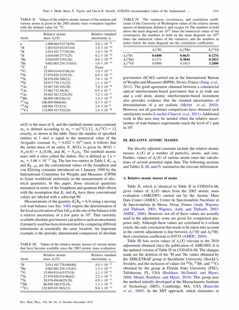
The directly adjusted constants include the relative atomicmasses ArðXÞ of a number of particles, atoms, and ions.Further, values of ArðXÞ of various atoms enter the calcula-tions of several potential input data. The following sectionsand Tables II, III, and IV summarize the relevant information.
A. Relative atomic masses of atoms
Table II, which is identical to Table II in CODATA-06,gives values of ArðXÞ taken from the 2003 atomic massevaluation (AME2003) carried out by the Atomic MassData Center (AMDC), Centre de Spectrometrie Nucleaire etde Spectrometrie de Masse, Orsay, France (Audi, Wapstra,and Thibault, 2003; Wapstra, Audi, and Thibault, 2003;AMDC, 2006). However, not all of these values are actuallyused in the adjustment; some are given for comparison pur-poses only. Although these values are correlated to a certainextent, the only correlation that needs to be taken into accountin the current adjustment is that between Arð1HÞ and Arð2HÞ;their correlation coefficient is 0.0735 (AMDC, 2003).
Table III lists seven values of ArðXÞ relevant to the 2010adjustment obtained since the publication of AME2003. It isthe updated version of Table IV in CODATA-06. The changesmade are the deletion of the 3H and 3He values obtained bythe SMILETRAP group at Stockholm University (StockU),Sweden; and the inclusion of values for 28Si, 87Rb, and 133Csobtained by the group at Florida State University (FSU),Tallahassee, FL, USA (Redshaw, McDaniel, and Myers,2008; Mount, Redshaw, and Myers, 2010). This group usesthe method initially developed at the Massachusetts Instituteof Technology (MIT), Cambridge, MA, USA (Rainvilleet al., 2005). In the MIT approach, which eliminates or
TABLE II. Values of the relative atomic masses of the neutron andvarious atoms as given in the 2003 atomic mass evaluation togetherwith the defined value for 12C.
AtomRelative atomicmass ArðXÞ
Relative standarduncertainty ur
n 1.008 664 915 74(56) 5:6� 10�10
1H 1.007 825 032 07(10) 1:0� 10�10
2H 2.014 101 777 85(36) 1:8� 10�10
3H 3.016 049 2777(25) 8:2� 10�10
3He 3.016 029 3191(26) 8:6� 10�10
4He 4.002 603 254 153(63) 1:6� 10�11
12C 12 Exact16O 15.994 914 619 56(16) 1:0� 10�11
28Si 27.976 926 5325(19) 6:9� 10�11
29Si 28.976 494 700(22) 7:6� 10�10
30Si 29.973 770 171(32) 1:1� 10�9
36Ar 35.967 545 105(28) 7:8� 10�10
38Ar 37.962 732 39(36) 9:5� 10�9
40Ar 39.962 383 1225(29) 7:2� 10�11
87Rb 86.909 180 526(12) 1:4� 10�10
107Ag 106.905 0968(46) 4:3� 10�8
109Ag 108.904 7523(31) 2:9� 10�8
133Cs 132.905 451 932(24) 1:8� 10�10
TABLE III. Values of the relative atomic masses of various atomsthat have become available since the 2003 atomic mass evaluation.
AtomRelative atomicmass ArðXÞ
Relative standarduncertainty ur
2H 2.014 101 778 040(80) 4:0� 10�11
4He 4.002 603 254 131(62) 1:5� 10�11
16O 15.994 914 619 57(18) 1:1� 10�11
28Si 27.976 926 534 96(62) 2:2� 10�11
29Si 28.976 494 6625(20) 6:9� 10�11
87Rb 86.909 180 535(10) 1:2� 10�10
133Cs 132.905 451 963(13) 9:8� 10�11
TABLE IV. The variances, covariances, and correlation coeffi-cients of the University of Washington values of the relative atomicmasses of deuterium, helium 4, and oxygen 16. The numbers in boldabove the main diagonal are 1020 times the numerical values of thecovariances; the numbers in bold on the main diagonal are 1020
times the numerical values of the variances; and the numbers initalics below the main diagonal are the correlation coefficients.
Arð2HÞ Arð4HeÞ Arð16OÞArð2HÞ 0:6400 0:0631 0:1276Arð4HeÞ 0.1271 0:3844 0:2023Arð16OÞ 0.0886 0.1813 3:2400
Peter J. Mohr, Barry N. Taylor, and David B. Newell: CODATA recommended values of the fundamental . . . 1531
Rev. Mod. Phys., Vol. 84, No. 4, October–December 2012
reduces a number of systematic effects and their associateduncertainties, mass ratios are determined by directly compar-ing the cyclotron frequencies of two different ions simulta-neously confined in a Penning trap. [The value of Arð29SiÞ inTable III is given in the supplementary information of the lastcited reference.]
The deleted SMILETRAP results are not discarded but areincluded in the adjustment in a more fundamental way, asdescribed in Sec. III.C. The values of Arð2HÞ, Arð4HeÞ, andArð16OÞ in Table III were obtained by the University ofWashington (UWash) group, Seattle, WA, USA, and wereused in the 2006 adjustment. The three values are correlatedand their variances, covariances, and correlation coefficientsare given in Table IV, which is identical to Table VI inCODATA-06.
The values of ArðXÞ from Table II initially used as inputdata for the 2010 adjustment are Arð1HÞ, Arð2HÞ, Arð87RbÞ,and Arð133CsÞ; and from Table III, Arð2HÞ, Arð4HeÞ, Arð16OÞ,Arð87RbÞ, and Arð133CsÞ. These values are items B1, B2:1,B2:2, and B7–B10:2 in Table XX, Sec. XIII. As in the 2006adjustment, the AME2003 values for Arð3HÞ, and Arð3HeÞ inTable II are not used because they were influenced by anearlier 3He result of the UWash group that disagrees withtheir newer, more accurate result (Van Dyck, 2010). Althoughnot yet published, it can be said that it agrees well with thevalue from the SMILETRAP group; see Sec. III.C.
Also as in the 2006 adjustment, the UWash group’s valuesfor Arð4HeÞ and Arð16OÞ in Table III are used in place of thecorresponding AME2003 values in Table II because the latterare based on a preliminary analysis of the data while thosein Table III are based on a thorough reanalysis of the data(Van Dyck, et al., 2006).
Finally, we note that the Arð2HÞ value of the UWash groupin Table III is the same as used in the 2006 adjustment. Asdiscussed in CODATA-06, it is a near-final result with aconservatively assigned uncertainty based on the analysis of10 runs taken over a 4-year period privately communicated tothe Task Group in 2006 by R. S. Van Dyck. A final resultcompletely consistent with it based on the analysis of 11 runsbut with an uncertainty of about half that given in the tableshould be published in due course together with the finalresult for Arð3HeÞ (Van Dyck, 2010).
B. Relative atomic masses of ions and nuclei
For a neutral atom X, ArðXÞ can be expressed in terms of Ar
of an ion of the atom formed by the removal of n electronsaccording to
ArðXÞ ¼ ArðXnþÞ þ nArðeÞ � EbðXÞ � EbðXnþÞmuc
2: (1)
In this expression, EbðXÞ=muc2 is the relative-atomic-mass
equivalent of the total binding energy of the Z electrons of theatom and Z is the atom’s atomic number (proton number).Similarly, EbðXnþÞ=muc
2 is the relative-atomic-mass equiva-lent of the binding energy of the Z� n electrons of the Xnþion. For an ion that is fully stripped n ¼ Z and XZþ is simplyN, the nucleus of the atom. In this case EbðXZþÞ=muc
2 ¼ 0and Eq. (1) becomes of the form of the first two equations ofTable XXXIII, Sec. XIII.
The binding energies Eb employed in the 2010 adjustmentare the same as those used in that of 2002 and 2006; seeTable IV of CODATA-02. However, the binding energy fortritium, 3H, is not included in that table. We employ the valueused in the 2006 adjustment, 1:097 185 439� 107 m�1, dueto Kotochigova (2006). For our purposes here, the uncertain-ties of the binding energies are negligible.
C. Relative atomic masses of the proton, triton, and helion
The focus of this section is the cyclotron frequency ratiomeasurements of the SMILETRAP group that lead to valuesof ArðpÞ, ArðtÞ, and ArðhÞ, where the triton t and helion h arethe nuclei of 3H and 3He. The reported values of Nagy et al.(2006) for Arð3HÞ and Arð3HeÞ were used as input data in the2006 adjustment but are not used in this adjustment. Instead,the actual cyclotron frequency ratio results underlying thosevalues are used as input data. This more fundamental way ofhandling the SMILETRAP group’s results is motivated by thesimilar but more recent work of the group related to theproton, which we discuss before considering the earlier work.
Solders et al. (2008) used the Penning-trap mass spec-trometer SMILETRAP, described in detail by Bergstromet al. (2002), to measure the ratio of the cyclotron frequencyfc of the H2
þ� molecular ion to that of the deuteron d, the
nucleus of the 2H atom. (The cyclotron frequency of an ion ofcharge q and mass m in a magnetic flux density B is given byfc ¼ qB=2�m.) Here the asterisk indicates that the singlyionized H2 molecules are in excited vibrational states as aresult of the 3.4 keV electrons used to bombard neutral H2
molecules in their vibrational ground state in order to ionizethem. The reported result is
fcðHþ�2 Þ
fcðdÞ ¼0:99923165933ð17Þ ½1:7�10�10�: (2)
This value was obtained using a two-pulse Ramsey tech-nique to excite the cyclotron frequencies, thereby enabling amore precise determination of the cyclotron resonance fre-quency line center than was possible with the one-pulseexcitation used in earlier work (George et al., 2007;Suhonen et al., 2007). The uncertainty is essentially allstatistical; components of uncertainty from systematic effectssuch as ‘‘q=A asymmetry’’ (difference of charge-to-massratio of the two ions), time variation of the 4.7 T appliedmagnetic flux density, relativistic mass increase, and ion-ioninteractions were deemed negligible by comparison.
The frequency ratio fcðH2þ�Þ=fcðdÞ can be expressed in
terms of adjusted constants and ionization and bindingenergies that have negligible uncertainties in this context.Based on Sec. III.B we can write
ArðH2Þ ¼ 2ArðHÞ � EBðH2Þ=muc2; (3)
ArðHÞ ¼ ArðpÞ þ ArðeÞ � EIðHÞ=muc2; (4)
ArðH2Þ ¼ ArðHþ2 Þ þ ArðeÞ � EIðH2Þ=muc
2; (5)
ArðHþ�2 Þ ¼ ArðHþ
2 Þ þ Eav=muc2; (6)
which yields
1532 Peter J. Mohr, Barry N. Taylor, and David B. Newell: CODATA recommended values of the fundamental . . .
Rev. Mod. Phys., Vol. 84, No. 4, October–December 2012
ArðHþ�2 Þ ¼ 2ArðpÞ þ ArðeÞ � EBðHþ�
2 Þ=muc2; (7)
where
EBðHþ�2 Þ ¼ 2EIðHÞ þ EBðH2Þ � EIðH2Þ � Eav (8)
is the binding energy of the Hþ�2 excited molecule. Here
EIðHÞ is the ionization energy of hydrogen, EBðH2Þ is thedisassociation energy of the H2 molecule, EIðH2Þ is the singleelectron ionization energy of H2, and Eav is the averagevibrational excitation energy of an Hþ
2 molecule as a result
of the ionization of H2 by 3.4 keV electron impact.The observational equation for the frequency ratio is thus
fcðHþ�2 Þ
fcðdÞ ¼ ArðdÞ2ArðpÞ þ ArðeÞ � EBðHþ�
2 Þ=muc2: (9)
We treat Eav as an adjusted constant in addition to ArðeÞ,ArðpÞ, and ArðdÞ in order to take its uncertainty into account ina consistent way, especially since it enters into the observa-tional equations for the frequency ratios to be discussedbelow.
The required ionization and binding energies as well as Eav
that we use are as given by Solders et al. (2008) and exceptfor Eav, have negligible uncertainties:
EIðHÞ ¼ 13:5984 eV ¼ 14:5985� 10�9muc2; (10)
EBðH2Þ ¼ 4:4781 eV ¼ 4:8074� 10�9muc2; (11)
EIðH2Þ ¼ 15:4258 eV ¼ 16:5602� 10�9muc2; (12)
Eav ¼ 0:740ð74Þ eV ¼ 0:794ð79Þ � 10�9muc2: (13)
We now consider the SMILETRAP results of Nagy et al.(2006) for the ratio of the cyclotron frequency of the triton tand of the 3Heþ ion to that of the H2
þ� molecular ion. They
report for the triton
fcðtÞfcðHþ�
2 Þ¼0:66824772686ð55Þ ½8:2�10�10� (14)
and for the 3Heþ ion
fcð3HeþÞfcðHþ�
2 Þ ¼0:66825214682ð55Þ ½8:2�10�10�: (15)
The relative uncertainty of the triton ratio consists of thefollowing uncertainty components in parts in 109: 0:22 sta-tistical, and 0.1, 0.1, 0.77, and 0.1 due to relativistic massshift, ion number dependence, q=A asymmetry, and contami-nant ions, respectively. The components for the 3Heþ ionratio are the same except the statistical uncertainty is 0.24. Allof these components are independent except the 0:77� 10�9
component due to q=A asymmetry; it leads to a correlationcoefficient between the two frequency ratios of 0.876.
Observational equations for these frequency ratios are
fcðtÞfcðHþ�
2 Þ ¼2ArðpÞ þ ArðeÞ � EBðHþ�
2 Þ=muc2
ArðtÞ (16)
and
fcð3HeþÞfcðHþ�
2 Þ ¼ 2ArðpÞ þ ArðeÞ � EBðHþ�2 Þ=muc
2
ArðhÞ þ ArðeÞ � EIð3HeþÞ=muc2; (17)
where
Arð3HeþÞ ¼ ArðhÞ þ ArðeÞ � EIð3HeþÞ=muc2 (18)
and
EIð3HeþÞ ¼ 51:4153 eV ¼ 58:4173� 10�9muc2 (19)
is the ionization energy of the 3Heþ ion, based on Table IVofCODATA-02.
The energy Eav and the three frequency ratios given inEqs. (2), (14), and (15), are items B3 to B6 in Table XX.
D. Cyclotron resonance measurement of the electron relative
atomic mass
As in the 2002 and 2006 CODATA adjustments, wetake as an input datum the Penning-trap result for theelectron relative atomic mass ArðeÞ obtained by theUniversity of Washington group (Farnham, Van Dyck, Jr.,and Schwinberg, 1995):
ArðeÞ¼0:000 548 579 9111ð12Þ ½2:1�10�9�: (20)
This is item B11 of Table XX.
IV. ATOMIC TRANSITION FREQUENCIES
Measurements and theory of transition frequencies in hy-drogen, deuterium, antiprotonic helium, and muonic hydro-gen provide information on the Rydberg constant, the protonand deuteron charge radii, and the relative atomic mass of theelectron. These topics as well as hyperfine and fine-structuresplittings are considered in this section.
A. Hydrogen and deuterium transition frequencies, the Rydberg
constant R1, and the proton and deuteron charge radii rp, rd
Transition frequencies between states a and b in hydrogenand deuterium are given by
�ab ¼ Eb � Ea
h; (21)
where Ea and Eb are the energy levels of the states. Theenergy levels divided by h are given by
Ea
h¼ ��2mec
2
2n2ahð1þ �aÞ ¼ �R1c
n2að1þ �aÞ; (22)
where R1c is the Rydberg constant in frequency units, na isthe principle quantum number of state a, and �a is a smallcorrection factor (j�aj � 1) that contains the details of thetheory of the energy level, including the effect of the finitesize of the nucleus as a function of the rms charge radius rpfor hydrogen or rd for deuterium. In the following summary,corrections are given in terms of the contribution to theenergy level, but in the numerical evaluation for the least-squares adjustment, R1 is factored out of the expressions andis an adjusted constant.
Peter J. Mohr, Barry N. Taylor, and David B. Newell: CODATA recommended values of the fundamental . . . 1533
Rev. Mod. Phys., Vol. 84, No. 4, October–December 2012
1. Theory of hydrogen and deuterium energy levels
Here we provide the information necessary to determinetheoretical values of the relevant energy levels, with theemphasis of the discussion on results that have become avail-able since the 2006 adjustment. For brevity, most referencesto earlier work, which can be found in Eides, Grotch, andShelyuto (2001b, 2007), for example, are not included here.
Theoretical values of the energy levels of different statesare highly correlated. In particular, uncalculated terms for Sstates are primarily of the form of an unknown commonconstant divided by n3. We take this fact into account bycalculating covariances between energy levels in addition tothe uncertainties of the individual levels (see Sec. IV.A.1.l).The correlated uncertainties are denoted by u0, while theuncorrelated uncertainties are denoted by un.
a. Dirac eigenvalue
The Dirac eigenvalue for an electron in a Coulomb field is
ED ¼ fðn; jÞmec2; (23)
where
fðn; jÞ ¼�1þ ðZ�Þ2
ðn� �Þ2��1=2
; (24)
n and j are the principal quantum number and total angularmomentum of the state, respectively, and
� ¼ jþ 1
2�
��jþ 1
2
�2 � ðZ�Þ2
�1=2
: (25)
In Eqs. (24) and (25), Z is the charge number of the nucleus,which for hydrogen and deuterium is 1. However, we shallretain Z as a parameter to classify the various contributions.
Equation (23) is valid only for an infinitely heavy nucleus.For a nucleus with a finite mass mN that expression isreplaced by (Barker and Glover, 1955; Sapirstein andYennie, 1990):
EMðHÞ ¼Mc2 þ ½fðn; jÞ � 1�mrc2 � ½fðn; jÞ � 1�2m
2r c
2
2M
þ 1��‘0
�ð2‘þ 1ÞðZ�Þ4m3
r c2
2n3m2N
þ �� � (26)
for hydrogen or by (Pachucki and Karshenboim, 1995)
EMðDÞ ¼Mc2 þ ½fðn; jÞ � 1�mrc2 � ½fðn; jÞ � 1�2m
2r c
2
2M
þ 1
�ð2‘þ 1ÞðZ�Þ4m3
r c2
2n3m2N
þ �� � (27)
for deuterium. In Eqs. (26) and (27) ‘ is the nonrelativisticorbital angular momentum quantum number, � ¼ð�1Þj�‘þ1=2ðjþ 1
2Þ is the angular-momentum-parity quantum
number, M ¼ me þmN, and mr ¼ memN=ðme þmNÞ is thereduced mass.
Equations (26) and (27) differ in that the Darwin-Foldyterm proportional to �‘0 is absent in Eq. (27), because it doesnot occur for a spin-one nucleus such as the deuteron(Pachucki and Karshenboim, 1995). In the three previousadjustments, Eq. (26) was used for both hydrogen and deu-terium and the absence of the Darwin-Foldy term in the case
of deuterium was accounted for by defining an effectivedeuteron radius given by Eq. (A56) of CODATA-98 and usingit to calculate the finite nuclear-size correction given byEq. (A43) and the related equations in that paper. The extraterm in the size correction canceled the Darwin-Foldy term inEq. (26); see also Sec. IV.A.1.h.
b. Relativistic recoil
The leading relativistic-recoil correction, to lowest order inZ� and all orders in me=mN, is (Erickson, 1977; Sapirsteinand Yennie, 1990)
ES ¼ m3r
m2emN
ðZ�Þ5�n3
mec2
�1
3�‘0 lnðZ�Þ�2 � 8
3lnk0ðn; ‘Þ
� 1
9�‘0 � 7
3an � 2
m2N �m2
e
�‘0
�m2
N ln
�me
mr
�
�m2e ln
�mN
mr
���; (28)
where
an ¼ �2
�ln
�2
n
�þXn
i¼1
1
iþ 1� 1
2n
��‘0
þ 1� �‘0
‘ð‘þ 1Þð2‘þ 1Þ : (29)
To lowest order in the mass ratio, the next two ordersin Z� are
ER ¼ me
mN
ðZ�Þ6n3
mec2½D60 þD72Z�ln
2ðZ�Þ�2 þ � � ��;(30)
where for nS1=2 states (Pachucki and Grotch, 1995; Eides and
Grotch, 1997c; Melnikov and Yelkhovsky, 1999; Pachuckiand Karshenboim, 1999)
D60 ¼ 4 ln2� 7
2; (31)
D72 ¼ � 11
60�; (32)
and for states with ‘ � 1 (Golosov et al., 1995; Elkhovski��,1996; Jentschura and Pachucki, 1996)
D60 ¼�3� ‘ð‘þ 1Þ
n2
�2
ð4‘2 � 1Þð2‘þ 3Þ : (33)
Based on the general pattern of the magnitudes of higher-order coefficients, the uncertainty for S states is taken to be10% of Eq. (30), and for states with ‘ � 1, it is taken to be1%. Numerical values for Eq. (30) to all orders in Z� havebeen obtained by Shabaev et al. (1998), and although theydisagree somewhat with the analytic result, they are consis-tent within the uncertainty assigned here. We employ theanalytic equations in the adjustment. The covariances of thetheoretical values are calculated by assuming that the uncer-tainties are predominately due to uncalculated terms propor-tional to ðme=mNÞ=n3.
1534 Peter J. Mohr, Barry N. Taylor, and David B. Newell: CODATA recommended values of the fundamental . . .
Rev. Mod. Phys., Vol. 84, No. 4, October–December 2012
c. Nuclear polarizability
For hydrogen, we use the result (Khriplovich and Sen’kov,2000)
EPðHÞ ¼ �0:070ð13Þh�l0
n3kHz: (34)
More recent results are a model calculation by Nevado andPineda (2008) and a slightly different result than Eq. (34)calculated by Martynenko (2006).
For deuterium, the sum of the proton polarizability, theneutron polarizibility (Khriplovich and Sen’kov, 1998), andthe dominant nuclear structure polarizibility (Friar and Payne,1997a), gives
EPðDÞ ¼ �21:37ð8Þh�l0
n3kHz: (35)
Presumably the polarization effect is negligible for statesof higher ‘ in either hydrogen or deuterium.
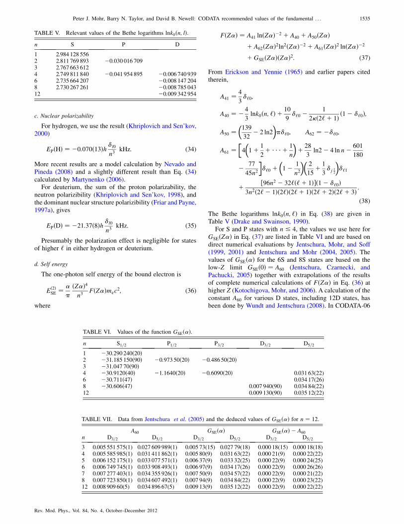
d. Self energy
The one-photon self energy of the bound electron is
Eð2ÞSE ¼ �
�
ðZ�Þ4n3
FðZ�Þmec2; (36)
where
FðZ�Þ ¼ A41 lnðZ�Þ�2 þ A40 þ A50ðZ�Þþ A62ðZ�Þ2ln2ðZ�Þ�2 þ A61ðZ�Þ2 lnðZ�Þ�2
þGSEðZ�ÞðZ�Þ2: (37)
From Erickson and Yennie (1965) and earlier papers citedtherein,
A41 ¼ 4
3�‘0;
A40 ¼ � 4
3lnk0ðn; ‘Þ þ 10
9�‘0 � 1
2�ð2‘þ 1Þ ð1� �‘0Þ;
A50 ¼�139
32� 2 ln2
���‘0; A62 ¼ ��‘0;
A61 ¼�4
�1þ 1
2þ � � � þ 1
n
�þ 28
3ln2� 4 ln n� 601
180
� 77
45n2
��‘0 þ
�1� 1
n2
��2
15þ 1
3�j 1
2
��‘1
þ ½96n2 � 32‘ð‘þ 1Þ�ð1� �‘0Þ3n2ð2‘� 1Þð2‘Þð2‘þ 1Þð2‘þ 2Þð2‘þ 3Þ :
(38)
The Bethe logarithms lnk0ðn; ‘Þ in Eq. (38) are given inTable V (Drake and Swainson, 1990).
For S and P states with n 4, the values we use here forGSEðZ�Þ in Eq. (37) are listed in Table VI and are based ondirect numerical evaluations by Jentschura, Mohr, and Soff(1999, 2001) and Jentschura and Mohr (2004, 2005). Thevalues of GSEð�Þ for the 6S and 8S states are based on thelow-Z limit GSEð0Þ ¼ A60 (Jentschura, Czarnecki, andPachucki, 2005) together with extrapolations of the resultsof complete numerical calculations of FðZ�Þ in Eq. (36) athigher Z (Kotochigova, Mohr, and 2006). A calculation of theconstant A60 for various D states, including 12D states, hasbeen done by Wundt and Jentschura (2008). In CODATA-06
TABLE V. Relevant values of the Bethe logarithms lnk0ðn; lÞ.n S P D
1 2.984 128 5562 2.811 769 893 �0:030 016 7093 2.767 663 6124 2.749 811 840 �0:041 954 895 �0:006 740 9396 2.735 664 207 �0:008 147 2048 2.730 267 261 �0:008 785 04312 �0:009 342 954
TABLE VI. Values of the function GSEð�Þ.n S1=2 P1=2 P3=2 D3=2 D5=2
1 �30:290 240ð20Þ2 �31:185 150ð90Þ �0:973 50ð20Þ �0:486 50ð20Þ3 �31:047 70ð90Þ4 �30:9120ð40Þ �1:1640ð20Þ �0:6090ð20Þ 0.031 63(22)6 �30:711ð47Þ 0.034 17(26)8 �30:606ð47Þ 0.007 940(90) 0.034 84(22)12 0.009 130(90) 0.035 12(22)
TABLE VII. Data from Jentschura et al. (2005) and the deduced values of GSEð�Þ for n ¼ 12.
A60 GSEð�Þ GSEð�Þ � A60
n D3=2 D5=2 D3=2 D5=2 D3=2 D5=2
3 0.005 551 575(1) 0.027 609 989(1) 0.005 73(15) 0.027 79(18) 0.000 18(15) 0.000 18(18)4 0.005 585 985(1) 0.031 411 862(1) 0.005 80(9) 0.031 63(22) 0.000 21(9) 0.000 22(22)5 0.006 152 175(1) 0.033 077 571(1) 0.006 37(9) 0.033 32(25) 0.000 22(9) 0.000 24(25)6 0.006 749 745(1) 0.033 908 493(1) 0.006 97(9) 0.034 17(26) 0.000 22(9) 0.000 26(26)7 0.007 277 403(1) 0.034 355 926(1) 0.007 50(9) 0.034 57(22) 0.000 22(9) 0.000 21(22)8 0.007 723 850(1) 0.034 607 492(1) 0.007 94(9) 0.034 84(22) 0.000 22(9) 0.000 23(22)12 0.008 909 60(5) 0.034 896 67(5) 0.009 13(9) 0.035 12(22) 0.000 22(9) 0.000 22(22)
Peter J. Mohr, Barry N. Taylor, and David B. Newell: CODATA recommended values of the fundamental . . . 1535
Rev. Mod. Phys., Vol. 84, No. 4, October–December 2012
this constant was obtained by extrapolation from lower-nstates. The more recent calculated values are
A60ð12D3=2Þ ¼ 0:008 909 60ð5Þ; (39)
A60ð12D5=2Þ ¼ 0:034 896 67ð5Þ: (40)
To estimate the corresponding value of GSEð�Þ, we use thedata from Jentschura et al. (2005) given in Table VII. It isevident from the table that
GSEð�Þ � A60 � 0:000 22 (41)
for the nD3=2 and nD5=2 states for n ¼ 4, 5, 6, 7, 8, so we
make the approximation
GSEð�Þ ¼ A60 þ 0:000 22; (42)
with an uncertainty given by 0.000 09 and 0.000 22 for the12D3=2 and 12D5=2 states, respectively. This yields
GSEð�Þ ¼ 0:000 130ð90Þ for 12D3=2; (43)
GSEð�Þ ¼ 0:035 12ð22Þ for 12D5=2: (44)
All values for GSEð�Þ that we use here are listed in Table VI.The uncertainty of the self-energy contribution to a givenlevel arises entirely from the uncertainty of GSEð�Þ listed inthat table and is taken to be type un.
The dominant effect of the finite mass of the nucleus on theself-energy correction is taken into account by multiplyingeach term of FðZ�Þ by the reduced-mass factor ðmr=meÞ3,except that the magnetic-moment term �1=½2�ð2‘þ 1Þ� inA40 is instead multiplied by the factor ðmr=meÞ2. In addition,the argument ðZ�Þ�2 of the logarithms is replaced byðme=mrÞðZ�Þ�2 (Sapirstein and Yennie, 1990).
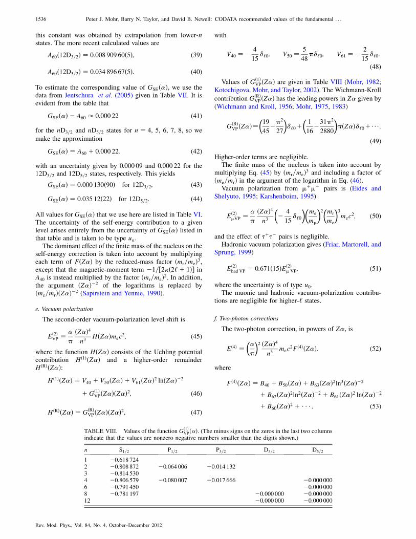
e. Vacuum polarization
The second-order vacuum-polarization level shift is
Eð2ÞVP ¼ �
�
ðZ�Þ4n3
HðZ�Þmec2; (45)
where the function HðZ�Þ consists of the Uehling potentialcontribution Hð1ÞðZ�Þ and a higher-order remainderHðRÞðZ�Þ:
Hð1ÞðZ�Þ ¼ V40 þ V50ðZ�Þ þ V61ðZ�Þ2 lnðZ�Þ�2
þ Gð1ÞVPðZ�ÞðZ�Þ2; (46)
HðRÞðZ�Þ ¼ GðRÞVPðZ�ÞðZ�Þ2; (47)
with
V40 ¼� 4
15�‘0; V50 ¼ 5
48��‘0; V61 ¼� 2
15�‘0:
(48)
Values of Gð1ÞVPðZ�Þ are given in Table VIII (Mohr, 1982;
Kotochigova, Mohr, and Taylor, 2002). The Wichmann-Kroll
contribution GðRÞVPðZ�Þ has the leading powers in Z� given by
(Wichmann and Kroll, 1956; Mohr, 1975, 1983)
GðRÞVPðZ�Þ¼
�19
45��2
27
��‘0þ
�1
16�31�2
2880
��ðZ�Þ�‘0þ���:
(49)
Higher-order terms are negligible.The finite mass of the nucleus is taken into account by
multiplying Eq. (45) by ðmr=meÞ3 and including a factor ofðme=mrÞ in the argument of the logarithm in Eq. (46).
Vacuum polarization from �þ�� pairs is (Eides andShelyuto, 1995; Karshenboim, 1995)
Eð2Þ�VP ¼ �
�
ðZ�Þ4n3
�� 4
15�‘0
��me
m�
�2�mr
me
�3mec
2; (50)
and the effect of �þ�� pairs is negligible.Hadronic vacuum polarization gives (Friar, Martorell, and
Sprung, 1999)
Eð2Þhad VP ¼ 0:671ð15ÞEð2Þ
� VP; (51)
where the uncertainty is of type u0.The muonic and hadronic vacuum-polarization contribu-
tions are negligible for higher-‘ states.
f. Two-photon corrections
The two-photon correction, in powers of Z�, is
Eð4Þ ¼��
�
�2 ðZ�Þ4
n3mec
2Fð4ÞðZ�Þ; (52)
where
Fð4ÞðZ�Þ ¼ B40 þ B50ðZ�Þ þ B63ðZ�Þ2ln3ðZ�Þ�2
þ B62ðZ�Þ2ln2ðZ�Þ�2 þ B61ðZ�Þ2 lnðZ�Þ�2
þ B60ðZ�Þ2 þ � � � : (53)
TABLE VIII. Values of the function Gð1ÞVPð�Þ. (The minus signs on the zeros in the last two columns
indicate that the values are nonzero negative numbers smaller than the digits shown.)
n S1=2 P1=2 P3=2 D3=2 D5=2
1 �0:618 7242 �0:808 872 �0:064 006 �0:014 1323 �0:814 5304 �0:806 579 �0:080 007 �0:017 666 �0:000 0006 �0:791 450 �0:000 0008 �0:781 197 �0:000 000 �0:000 00012 �0:000 000 �0:000 000
1536 Peter J. Mohr, Barry N. Taylor, and David B. Newell: CODATA recommended values of the fundamental . . .
Rev. Mod. Phys., Vol. 84, No. 4, October–December 2012
The leading term B40 is
B40¼�3�2
2ln2�10�2
27�2179
648�9
4ð3Þ
��‘0
þ��2 ln2
2��2
12�197
144�3ð3Þ
4
�1��‘0
�ð2‘þ1Þ ; (54)
where is the Riemann zeta function (Olver et al., 2010), andthe next term is (Pachucki, 1993a, 1994; Eides and Shelyuto,1995; Eides,Grotch, andShelyuto, 1997;Dowling et al., 2010)
B50 ¼ �21:554 47ð13Þ�‘0: (55)
The leading sixth-order coefficient is (Karshenbo��m, 1993;Manohar and Stewart, 2000; Yerokhin, 2000; Pachucki, 2001)
B63 ¼ � 8
27�‘0: (56)
For S states B62 is (Karshenboim, 1996; Pachucki, 2001)
B62¼16
9
�71
60� ln2þ�þc ðnÞ� lnn�1
nþ 1
4n2
�; (57)
where � ¼ 0:577 . . . is Euler’s constant and c is the psifunction (Olver et al., 2010). For P states (Karshenboim,1996; Jentschura and Nandori, 2002)
B62 ¼ 4
27
n2 � 1
n2; (58)
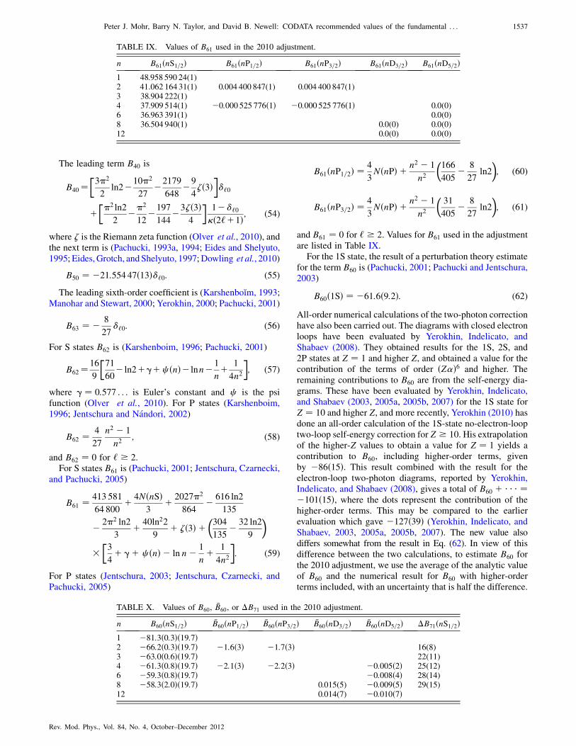
and B62 ¼ 0 for ‘ � 2.For S states B61 is (Pachucki, 2001; Jentschura, Czarnecki,
and Pachucki, 2005)
B61 ¼ 413 581
64 800þ 4NðnSÞ
3þ 2027�2
864� 616 ln2
135
� 2�2 ln2
3þ 40ln22
9þ ð3Þ þ
�304
135� 32 ln2
9
�
��3
4þ �þ c ðnÞ � ln n� 1
nþ 1
4n2
�: (59)
For P states (Jentschura, 2003; Jentschura, Czarnecki, andPachucki, 2005)
B61ðnP1=2Þ ¼ 4
3NðnPÞ þ n2 � 1
n2
�166
405� 8
27ln2
�; (60)
B61ðnP3=2Þ ¼ 4
3NðnPÞ þ n2 � 1
n2
�31
405� 8
27ln2
�; (61)
and B61 ¼ 0 for ‘ � 2. Values for B61 used in the adjustmentare listed in Table IX.
For the 1S state, the result of a perturbation theory estimatefor the term B60 is (Pachucki, 2001; Pachucki and Jentschura,2003)
B60ð1SÞ ¼ �61:6ð9:2Þ: (62)
All-order numerical calculations of the two-photon correctionhave also been carried out. The diagrams with closed electronloops have been evaluated by Yerokhin, Indelicato, andShabaev (2008). They obtained results for the 1S, 2S, and2P states at Z ¼ 1 and higher Z, and obtained a value for thecontribution of the terms of order ðZ�Þ6 and higher. Theremaining contributions to B60 are from the self-energy dia-grams. These have been evaluated by Yerokhin, Indelicato,and Shabaev (2003, 2005a, 2005b, 2007) for the 1S state forZ ¼ 10 and higher Z, and more recently, Yerokhin (2010) hasdone an all-order calculation of the 1S-state no-electron-looptwo-loop self-energy correction for Z � 10. His extrapolationof the higher-Z values to obtain a value for Z ¼ 1 yields acontribution to B60, including higher-order terms, givenby �86ð15Þ. This result combined with the result for theelectron-loop two-photon diagrams, reported by Yerokhin,Indelicato, and Shabaev (2008), gives a total of B60 þ � � � ¼�101ð15Þ, where the dots represent the contribution of thehigher-order terms. This may be compared to the earlierevaluation which gave �127ð39Þ (Yerokhin, Indelicato, andShabaev, 2003, 2005a, 2005b, 2007). The new value alsodiffers somewhat from the result in Eq. (62). In view of thisdifference between the two calculations, to estimate B60 forthe 2010 adjustment, we use the average of the analytic valueof B60 and the numerical result for B60 with higher-orderterms included, with an uncertainty that is half the difference.
TABLE IX. Values of B61 used in the 2010 adjustment.
n B61ðnS1=2Þ B61ðnP1=2Þ B61ðnP3=2Þ B61ðnD3=2Þ B61ðnD5=2Þ1 48.958 590 24(1)2 41.062 164 31(1) 0.004 400 847(1) 0.004 400 847(1)3 38.904 222(1)4 37.909 514(1) �0:000 525 776ð1Þ �0:000 525 776ð1Þ 0.0(0)6 36.963 391(1) 0.0(0)8 36.504 940(1) 0.0(0) 0.0(0)12 0.0(0) 0.0(0)
TABLE X. Values of B60, �B60, or �B71 used in the 2010 adjustment.
n B60ðnS1=2Þ �B60ðnP1=2Þ �B60ðnP3=2Þ �B60ðnD3=2Þ �B60ðnD5=2Þ �B71ðnS1=2Þ1 �81:3ð0:3Þð19:7Þ2 �66:2ð0:3Þð19:7Þ �1:6ð3Þ �1:7ð3Þ 16(8)3 �63:0ð0:6Þð19:7Þ 22(11)4 �61:3ð0:8Þð19:7Þ �2:1ð3Þ �2:2ð3Þ �0:005ð2Þ 25(12)6 �59:3ð0:8Þð19:7Þ �0:008ð4Þ 28(14)8 �58:3ð2:0Þð19:7Þ 0.015(5) �0:009ð5Þ 29(15)12 0.014(7) �0:010ð7Þ
Peter J. Mohr, Barry N. Taylor, and David B. Newell: CODATA recommended values of the fundamental . . . 1537
Rev. Mod. Phys., Vol. 84, No. 4, October–December 2012
The higher-order contribution is small compared to the dif-ference between the results of the two methods of calculation.The average result is
B60ð1SÞ ¼ �81:3ð0:3Þð19:7Þ: (63)
In Eq. (63), the first number in parentheses is the state-dependent uncertainty unðB60Þ associated with the two-loopBethe logarithm, and the second number in parentheses is thestate-independent uncertainty u0ðB60Þ that is common to allS-state values of B60. Two-loop Bethe logarithms needed toevaluate B60ðnSÞ have been given for n ¼ 1 to 6 (Pachuckiand Jentschura, 2003; Jentschura, 2004), and a value at n ¼ 8may be obtained by a simple extrapolation from the calcu-lated values [see Eq. (43) of CODATA-06]. The completestate dependence of B60ðnSÞ in terms of the two-loop Bethelogarithms has been calculated by Czarnecki, Jentschura, andPachucki (2005) and Jentschura, Czarnecki, and Pachucki(2005). Values of B60 for all relevant S states are given inTable X.
For higher-‘ states, an additional consideration is neces-sary. The radiative level shift includes contributions associ-ated with decay to lower levels. At the one-loop level, this isthe imaginary part of the level shift corresponding to theresonance scattering width of the level. At the two-loop levelthere is an imaginary contribution corresponding to two-photon decays and radiative corrections to the one-photondecays, but in addition there is a real contribution from thesquare of the one-photon decay width. This can be thought ofas the second-order term that arises in the expansion of theresonance denominator for scattering of photons from theatom in its ground state in powers of the level width(Jentschura et al., 2002). As such, this term should not beincluded in the calculation of the resonant line-center shiftof the scattering cross section, which is the quantity of interestfor the least-squares adjustment. The leading contribution ofthe square of the one-photon width is of order�ðZ�Þ6mec
2=ℏ.This correction vanishes for the 1S and 2S states, because the1S level has no width and the 2S level can only decay withtransition rates that are higher order in � and/or Z�. Thehigher-n S states have a contribution from the square of theone-photon width from decays to lower P states, but for the 3Sand 4S states for which it has been separately identified, thiscorrection is negligible compared to the uncertainty in B60
(Jentschura, 2004, 2006). We assume the correction for higherS states is also negligible compared to the numerical uncer-tainty in B60. However, the correction is taken into account inthe 2010 adjustment for P and D states for which it is relativelylarger (Jentschura et al., 2002; Jentschura, 2006).
Calculations of B60 for higher-‘ states have been made byJentschura (2006). The results can be expressed as
B60ðnLjÞ ¼ aðnLjÞ þ bLðnLÞ; (64)
where aðnLjÞ is a precisely calculated term that depends on j,
and the two-loop Bethe logarithm bLðnLÞ has a larger nu-merical uncertainty but does not depend on j. Jentschura(2006) gives semianalytic formulas for aðnLjÞ that includenumerically calculated terms. The information needed for the2010 adjustment is in Eqs. (22a), (22b), (23a), and (23b),Tables VII, VIII, IX, and X of Jentschura (2006) and Eq. (17)of Jentschura (2003). Two corrections to Eq. (22b) are
� 73 321
103 680þ 185
1152nþ 8111
25 920n2
! � 14 405
20 736þ 185
1152nþ 1579
5184n2(65)
on the first line and
� 3187
3600n2! þ 3187
3600n2(66)
on the fourth line (Jentschura, 2011a).Values of the two-photon Bethe logarithm bLðnLÞ may be
divided into a contribution of the ‘‘squared level width’’ term�2B60 and the rest �bLðnLÞ, so that
bLðnLÞ ¼ �2B60 þ �bLðnLÞ: (67)
The corresponding value �B60 that represents the shift of thelevel center is given by
�B60ðnLjÞ ¼ aðnLjÞ þ �bLðnLÞ: (68)
Here we give the numerical values for �BðnLjÞ in Table X and
refer the reader to Jentschura (2006) for the separate valuesfor aðnLjÞ and �bLðnLÞ. The D-state values for n ¼ 6, 8 are
extrapolated from the corresponding values at n ¼ 5, 6 with afunction of the form aþ b=n. The values in Table X for Sstates may be regarded as being either B60 or �B60, since thedifference is expected to be smaller than the uncertainty. Theuncertainties listed for the P- and D-state values of �BðnLjÞ inthat table are predominately from the two-photon Bethelogarithm which depends on n and L, but not on j for a givenn, L. Therefore there is a large covariance between thecorresponding two values of �BðnLjÞ. However, we do not
take this into consideration when calculating the uncertaintyin the fine-structure splitting, because the uncertainty ofhigher-order coefficients dominates over any improvementin accuracy the covariance would provide. We assume that theuncertainties in the two-photon Bethe logarithms are suffi-ciently large to account for higher-order P- and D-state two-photon uncertainties as well.
For S states, higher-order terms have been estimated byJentschura, Czarnecki, and Pachucki (2005) with an effectivepotential model. They find that the next term has a coefficientof B72 and is state independent. We thus assume that theuncertainty u0½B60ðnSÞ� is sufficient to account for the uncer-tainty due to omitting such a term and higher-order state-independent terms. In addition, they find an estimate for thestate dependence of the next term, given by
�B71ðnSÞ¼B71ðnSÞ�B71ð1SÞ¼�
�427
36�16
3ln2
�
��3
4� 1
nþ 1
4n2þ�þ c ðnÞ� lnn
�; (69)
with a relative uncertainty of 50%. We include this additionalterm, which is listed in Table X, along with the estimateduncertainty unðB71Þ ¼ B71=2.
1538 Peter J. Mohr, Barry N. Taylor, and David B. Newell: CODATA recommended values of the fundamental . . .
Rev. Mod. Phys., Vol. 84, No. 4, October–December 2012
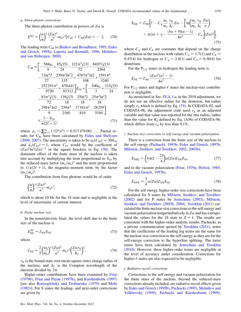
g. Three-photon corrections
The three-photon contribution in powers of Z� is
Eð6Þ ¼��
�
�3 ðZ�Þ4
n3mec
2½C40 þ C50ðZ�Þ þ � � ��: (70)
The leading term C40 is (Baikov and Broadhurst, 1995; Eidesand Grotch, 1995a; Laporta and Remiddi, 1996; Melnikovand van Ritbergen, 2000)
C40¼��568a4
9þ85ð5Þ
24�121�2ð3Þ
72�84071ð3Þ
2304
�71ln42
27�239�2ln22
135þ4787�2 ln2
108þ1591�4
3240
�252251�2
9720þ679441
93312
��‘0þ
��100a4
3þ215ð5Þ
24
�83�2ð3Þ72
�139ð3Þ18
�25ln42
18þ25�2ln22
18
þ298�2 ln2
9þ239�4
2160�17101�2
810�28259
5184
�
� 1��‘0
�ð2‘þ1Þ ; (71)
where a4 ¼P1
n¼1 1=ð2nn4Þ ¼ 0:517 479 061 . . . . Partial re-
sults for C50 have been calculated by Eides and Shelyuto(2004, 2007). The uncertainty is taken to be u0ðC50Þ ¼ 30�‘0
and unðC63Þ ¼ 1, where C63 would be the coefficient ofðZ�Þ2ln3ðZ�Þ�2 in the square brackets in Eq. (70). Thedominant effect of the finite mass of the nucleus is takeninto account by multiplying the term proportional to �‘0 bythe reduced-mass factor ðmr=meÞ3 and the term proportionalto 1=�ð2‘þ 1Þ, the magnetic-moment term, by the factorðmr=meÞ2.
The contribution from four photons would be of order
��
�
�4 ðZ�Þ4
n3mec
2; (72)
which is about 10 Hz for the 1S state and is negligible at thelevel of uncertainty of current interest.
h. Finite nuclear size
In the nonrelativistic limit, the level shift due to the finitesize of the nucleus is
Eð0ÞNS ¼ ENS�‘0; (73)
where
ENS ¼ 2
3
�mr
me
�3 ðZ�Þ2
n3mec
2
�Z�rNC
�2; (74)
rN is the bound-state root-mean-square (rms) charge radius ofthe nucleus, and C is the Compton wavelength of theelectron divided by 2�.
Higher-order contributions have been examined by Friar(1979b), Friar and Payne (1997b), and Karshenboim (1997)[see also Borisoglebsky and Trofimenko (1979) and Mohr(1983)]. For S states the leading- and next-order correctionsare given by
ENS ¼ ENS
�1� C�
mr
me
rNC
Z���ln
�mr
me
rNC
Z�
n
�
þ c ðnÞ þ �� ð5nþ 9Þðn� 1Þ4n2
� C�
�ðZ�Þ2
�;
(75)
where C� and C� are constants that depend on the charge
distribution in the nucleus with values C� ¼ 1:7ð1Þ and C� ¼0:47ð4Þ for hydrogen or C� ¼ 2:0ð1Þ and C� ¼ 0:38ð4Þ fordeuterium.
For the P1=2 states in hydrogen the leading term is
ENS ¼ ENS
ðZ�Þ2ðn2 � 1Þ4n2
: (76)
For P3=2 states and higher-‘ states the nuclear-size contribu-
tion is negligible.As mentioned in Sec. IV.A.1.a, in the 2010 adjustment, we
do not use an effective radius for the deuteron, but rathersimply rd which is defined by Eq. (74). In CODATA-02, andCODATA-06, the adjustment code used rd as an adjustedvariable and that value was reported for the rms radius, ratherthan the value for Rd defined by Eq. (A56) of CODATA-98,which differs from rd by less than 0.1%.
i. Nuclear-size correction to self energy and vacuum polarization
There is a correction from the finite size of the nucleus tothe self energy (Pachucki, 1993b; Eides and Grotch, 1997b;Milstein, Sushkov, and Terekhov, 2002, 2003b),
ENSE ¼�4 ln2� 23
4
��ðZ�ÞENS�‘0; (77)
and to the vacuum polarization (Friar, 1979a; Hylton, 1985;Eides and Grotch, 1997b),
ENVP ¼ 3
4�ðZ�ÞENS�‘0: (78)
For the self energy, higher-order size corrections have beencalculated for S states by Milstein, Sushkov, and Terekhov(2002) and for P states by Jentschura (2003), Milstein,Sushkov, and Terekhov (2003b, 2004). Yerokhin (2011) cal-culated the finite nuclear-size corrections to the self energy andvacuum polarization nonperturbatively inZ� and has extrapo-lated the values for the 1S state to Z ¼ 1. The results areconsistent with the higher-order analytic results. Pachucki, ina private communication quoted by Yerokhin (2011), notesthat the coefficients of the leading log terms are the same forthe nuclear-size correction to the self energy as they are for theself-energy correction to the hyperfine splitting. The latterterms have been calculated by Jentschura and Yerokhin(2010). However, these higher-order terms are negligible atthe level of accuracy under consideration. Corrections forhigher-‘ states are also expected to be negligible.
j. Radiative-recoil corrections
Corrections to the self energy and vacuum polarization forthe finite mass of the nucleus, beyond the reduced-masscorrections already included, are radiative-recoil effects givenby Eides and Grotch (1995b), Pachucki (1995), Melnikov andYelkhovsky (1999), Pachucki and Karshenboim (1999),
Peter J. Mohr, Barry N. Taylor, and David B. Newell: CODATA recommended values of the fundamental . . . 1539
Rev. Mod. Phys., Vol. 84, No. 4, October–December 2012
Czarnecki and Melnikov (2001), and Eides, Grotch, andShelyuto (2001a):
ERR¼ m3r
m2emN
�ðZ�Þ5�2n3
mec2�‘0
�6ð3Þ�2�2 ln2þ35�2
36
�448
27þ2
3�ðZ�Þln2ðZ�Þ�2þ���
�: (79)
The uncertainty is taken to be the term ðZ�Þ lnðZ�Þ�2 relativeto the square brackets with numerical coefficients 10 for u0and 1 for un. Corrections for higher-‘ states are expected tobe negligible.
k. Nucleus self energy
A correction due to the self energy of the nucleus is(Pachucki, 1995; Eides, Grotch, and Shelyuto, 2001b)
ESEN¼4Z2�ðZ�Þ43�n3
m3r
m2N
c2�ln
�mN
mrðZ�Þ2��‘0� lnk0ðn;‘Þ
�:
(80)
For the uncertainty, we assign a value to u0 corresponding toan additive constant of 0.5 in the square brackets in Eq. (80)for S states. For higher-‘ states, the correction is not included.
l. Total energy and uncertainty
The energy EXðnLjÞ of a level (where L ¼ S;P; . . . and
X ¼ H, D) is the sum of the various contributions listed in thepreceding sections plus an additive correction �XðnLjÞ that iszero with an uncertainty that is the rms sum of the uncertain-ties of the individual contributions:
u2½�XðnLjÞ� ¼Xi
u20iðXLjÞ þ u2niðXLjÞn6
; (81)
where u0iðXLjÞ=n3 and uniðXLjÞ=n3 are the components of
uncertainty u0 and un of contribution i. Uncertainties fromthe fundamental constants are not explicitly included here,because they are taken into account through the least-squaresadjustment.
The covariance of any two �’s follows from Eq. (F7) ofAppendix F of CODATA-98. For a given isotope
u½�Xðn1LjÞ; �Xðn2LjÞ� ¼Xi
u20iðXLjÞðn1n2Þ3
; (82)
which follows from the fact that uðu0i; uniÞ ¼ 0 anduðun1i; un2iÞ ¼ 0 for n1 � n2. We also assume that
u½�Xðn1L1j1 Þ; �Xðn2L2j2Þ� ¼ 0 (83)
if L1 � L2 or j1 � j2.For covariances between �’s for hydrogen and deuterium,
we have for states of the same n
u½�HðnLjÞ;�DðnLjÞ�
¼ Xi¼ficg
u0iðHLjÞu0iðDLjÞþuniðHLjÞuniðDLjÞn6
; (84)
and for n1 � n2
u½�Hðn1LjÞ; �Dðn2LjÞ� ¼Xi¼ic
u0iðHLjÞu0iðDLjÞðn1n2Þ3
; (85)
where the summation is over the uncertainties common tohydrogen and deuterium. We assume
u½�Hðn1L1j1Þ; �Dðn2L2j2 Þ� ¼ 0 (86)
if L1 � L2 or j1 � j2.The values of u½�XðnLjÞ� of interest for the 2010 adjust-
ment are given in Table XVIII of Sec. XIII, and the non-negligible covariances of the �’s are given as correlationcoefficients in Table XIX of that section. These coefficientsare as large as 0.9999.
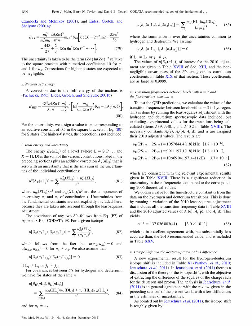
m. Transition frequencies between levels with n ¼ 2 and
the fine-structure constant �
To test the QED predictions, we calculate the values of thetransition frequencies between levels with n ¼ 2 in hydrogen.This is done by running the least-squares adjustment with thehydrogen and deuterium spectroscopic data included, butexcluding experimental values for the transitions being cal-culated (items A39, A40:1, and A40:2 in Table XVIII). Thenecessary constants ArðeÞ, ArðpÞ, ArðdÞ, and � are assignedtheir 2010 adjusted values. The results are
�Hð2P1=2�2S1=2Þ¼1057844:4ð1:8ÞkHz ½1:7�10�6�;�Hð2S1=2�2P3=2Þ¼9911197:1ð1:8ÞkHz ½1:8�10�7�;�Hð2P1=2�2P3=2Þ¼10969041:571ð41ÞkHz ½3:7�10�9�;
(87)
which are consistent with the relevant experimental resultsgiven in Table XVIII. There is a significant reduction inuncertainty in these frequencies compared to the correspond-ing 2006 theoretical values.
We obtain a value for the fine-structure constant � from thedata on the hydrogen and deuterium transitions. This is doneby running a variation of the 2010 least-squares adjustmentthat includes all the transition-frequency data in Table XVIIIand the 2010 adjusted values of ArðeÞ, ArðpÞ, and ArðdÞ. Thisyields
��1 ¼ 137:036 003ð41Þ ½3:0� 10�7�; (88)
which is in excellent agreement with, but substantially lessaccurate than, the 2010 recommended value, and is includedin Table XXV.
n. Isotope shift and the deuteron-proton radius difference
A new experimental result for the hydrogen-deuteriumisotope shift is included in Table XI (Parthey et al., 2010;Jentschura et al., 2011). In Jentschura et al. (2011) there is adiscussion of the theory of the isotope shift, with the objectiveof extracting the difference of the squares of the charge radiifor the deuteron and proton. The analysis in Jentschura et al.(2011) is in general agreement with the review given in thepreceding sections of the present work, with a few differencesin the estimates of uncertainties.
As pointed out by Jentschura et al. (2011), the isotope shiftis roughly given by
1540 Peter J. Mohr, Barry N. Taylor, and David B. Newell: CODATA recommended values of the fundamental . . .
Rev. Mod. Phys., Vol. 84, No. 4, October–December 2012
�f1S�2S;d � �f1S�2S;p � � 3
4R1c
�me
md
� me
mp
�
¼ 3
4R1c
meðmd �mpÞmdmp
; (89)
and from a comparison of experiment and theory, they obtain
r2d � r2p ¼ 3:820 07ð65Þ fm2 (90)
for the difference of the squares of the radii. This can becompared to the result given by the 2010 adjustment:
r2d � r2p ¼ 3:819 89ð42Þ fm2; (91)
which is in good agreement. (The difference of the squares ofthe quoted 2010 recommended values of the radii gives 87in the last two digits of the difference, rather than 89, dueto rounding.) The uncertainty follows from Eqs. (F11) and(F12) of CODATA-98. Here there is a significant reductionin the uncertainty compared to the uncertainties of theindividual radii because of the large correlation coefficient(physics.nist.gov/constants)
rðrd; rpÞ ¼ 0:9989: (92)
Part of the reduction in uncertainty in Eq. (91) compared toEq. (90) is due to the fact that the correlation coefficient takesinto account the covariance of the electron-nucleon massratios in Eq. (89).
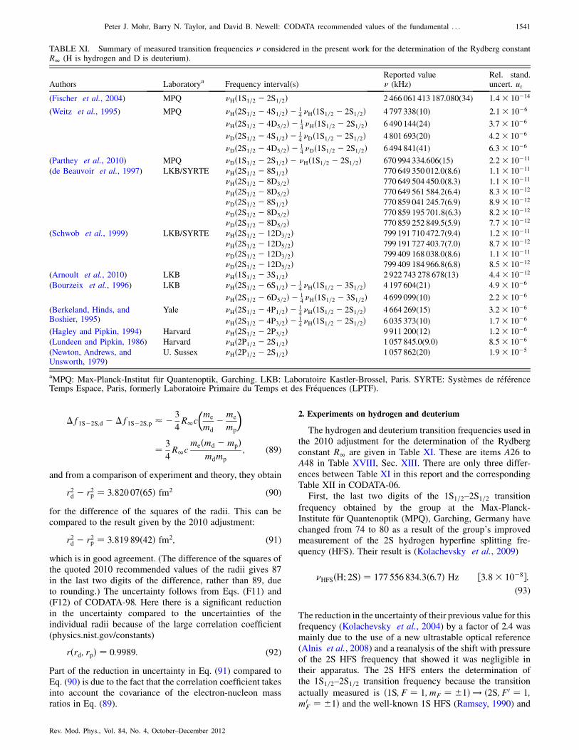
2. Experiments on hydrogen and deuterium
The hydrogen and deuterium transition frequencies used inthe 2010 adjustment for the determination of the Rydbergconstant R1 are given in Table XI. These are items A26 toA48 in Table XVIII, Sec. XIII. There are only three differ-ences between Table XI in this report and the correspondingTable XII in CODATA-06.
First, the last two digits of the 1S1=2–2S1=2 transition
frequency obtained by the group at the Max-Planck-Institute fur Quantenoptik (MPQ), Garching, Germany havechanged from 74 to 80 as a result of the group’s improvedmeasurement of the 2S hydrogen hyperfine splitting fre-quency (HFS). Their result is (Kolachevsky et al., 2009)
�HFSðH; 2SÞ ¼ 177 556 834:3ð6:7Þ Hz ½3:8� 10�8�:(93)
The reduction in the uncertainty of their previous value for thisfrequency (Kolachevsky et al., 2004) by a factor of 2.4 wasmainly due to the use of a new ultrastable optical reference(Alnis et al., 2008) and a reanalysis of the shift with pressureof the 2S HFS frequency that showed it was negligible intheir apparatus. The 2S HFS enters the determination ofthe 1S1=2–2S1=2 transition frequency because the transition
actually measured is ð1S; F ¼ 1; mF ¼ 1Þ ! ð2S; F0 ¼ 1;m0
F ¼ 1Þ and the well-known 1S HFS (Ramsey, 1990) and
TABLE XI. Summary of measured transition frequencies � considered in the present work for the determination of the Rydberg constantR1 (H is hydrogen and D is deuterium).
Authors Laboratorya
Frequency interval(s)Reported value� (kHz)
Rel. stand.uncert. ur
(Fischer et al., 2004) MPQ �Hð1S1=2 � 2S1=2Þ 2 466 061 413 187.080(34) 1:4� 10�14
(Weitz et al., 1995) MPQ �Hð2S1=2 � 4S1=2Þ � 14�Hð1S1=2 � 2S1=2Þ 4 797 338(10) 2:1� 10�6
�Hð2S1=2 � 4D5=2Þ � 14�Hð1S1=2 � 2S1=2Þ 6 490 144(24) 3:7� 10�6
�Dð2S1=2 � 4S1=2Þ � 14�Dð1S1=2 � 2S1=2Þ 4 801 693(20) 4:2� 10�6
�Dð2S1=2 � 4D5=2Þ � 14�Dð1S1=2 � 2S1=2Þ 6 494 841(41) 6:3� 10�6
(Parthey et al., 2010) MPQ �Dð1S1=2 � 2S1=2Þ � �Hð1S1=2 � 2S1=2Þ 670 994 334.606(15) 2:2� 10�11
(de Beauvoir et al., 1997) LKB/SYRTE �Hð2S1=2 � 8S1=2Þ 770 649 350 012.0(8.6) 1:1� 10�11
�Hð2S1=2 � 8D3=2Þ 770 649 504 450.0(8.3) 1:1� 10�11
�Hð2S1=2 � 8D5=2Þ 770 649 561 584.2(6.4) 8:3� 10�12
�Dð2S1=2 � 8S1=2Þ 770 859 041 245.7(6.9) 8:9� 10�12
�Dð2S1=2 � 8D3=2Þ 770 859 195 701.8(6.3) 8:2� 10�12
�Dð2S1=2 � 8D5=2Þ 770 859 252 849.5(5.9) 7:7� 10�12
(Schwob et al., 1999) LKB/SYRTE �Hð2S1=2 � 12D3=2Þ 799 191 710 472.7(9.4) 1:2� 10�11
�Hð2S1=2 � 12D5=2Þ 799 191 727 403.7(7.0) 8:7� 10�12
�Dð2S1=2 � 12D3=2Þ 799 409 168 038.0(8.6) 1:1� 10�11
�Dð2S1=2 � 12D5=2Þ 799 409 184 966.8(6.8) 8:5� 10�12
(Arnoult et al., 2010) LKB �Hð1S1=2 � 3S1=2Þ 2 922 743 278 678(13) 4:4� 10�12
(Bourzeix et al., 1996) LKB �Hð2S1=2 � 6S1=2Þ � 14�Hð1S1=2 � 3S1=2Þ 4 197 604(21) 4:9� 10�6
�Hð2S1=2 � 6D5=2Þ � 14�Hð1S1=2 � 3S1=2Þ 4 699 099(10) 2:2� 10�6
(Berkeland, Hinds, andBoshier, 1995)
Yale �Hð2S1=2 � 4P1=2Þ � 14�Hð1S1=2 � 2S1=2Þ 4 664 269(15) 3:2� 10�6
�Hð2S1=2 � 4P3=2Þ � 14�Hð1S1=2 � 2S1=2Þ 6 035 373(10) 1:7� 10�6
(Hagley and Pipkin, 1994) Harvard �Hð2S1=2 � 2P3=2Þ 9 911 200(12) 1:2� 10�6
(Lundeen and Pipkin, 1986) Harvard �Hð2P1=2 � 2S1=2Þ 1 057 845.0(9.0) 8:5� 10�6
(Newton, Andrews, andUnsworth, 1979)
U. Sussex �Hð2P1=2 � 2S1=2Þ 1 057 862(20) 1:9� 10�5
aMPQ: Max-Planck-Institut fur Quantenoptik, Garching. LKB: Laboratoire Kastler-Brossel, Paris. SYRTE: Systemes de referenceTemps Espace, Paris, formerly Laboratoire Primaire du Temps et des Frequences (LPTF).
Peter J. Mohr, Barry N. Taylor, and David B. Newell: CODATA recommended values of the fundamental . . . 1541
Rev. Mod. Phys., Vol. 84, No. 4, October–December 2012
the 2S HFS are required to convert the measured frequency to
the frequency of the hyperfine centroid.For completeness, we note that the MPQ group has very
recently reported a new value for the 1S1=2–2S1=2 transition
frequency that has an uncertainty of 10 Hz, corresponding to a
relative standard uncertainty of 4:2� 10�15, or about 30% of
the uncertainty of the value in the table (Parthey et al., 2011).Second, the previousMPQvalue (Huber et al., 1998) for the
hydrogen-deuterium 1S–2S isotope shift, that is, the frequency
difference �Dð1S1=2–2S1=2Þ � �Hð1S1=2–2S1=2Þ, has been re-
placed by their recent, much more accurate value (Parthey
et al., 2010); its uncertainty of 15 Hz, corresponding to a
relative uncertainty of 2:2� 10�11, is a factor of 10 smaller
than the uncertainty of their previous result. Many experimen-
tal advances enabled this significant uncertainty reduction, not
the least of which was the use of a fiber frequency comb
referenced to an active hydrogen maser steered by the
Global Positioning System (GPS) to measure laser frequen-
cies. The principal uncertainty components in the measure-
ment are 11 Hz due to density effects in the atomic beam, 6 Hz
from second-order Doppler shift, and 5.1 Hz statistical.Third, Table XI includes a new result from the group
at the Laboratoire Kastler-Brossel (LKB), Ecole Normale
Superieure et Universite Pierre et Marie Curie, Paris,
France. These researchers have extended their previous
work and determined the 1S1=2–3S1=2 transition frequency
in hydrogen using Doppler-free two-photon spectroscopy
with a relative uncertainty of 4:4� 10�12 (Arnoult et al.,
2010), the second smallest uncertainty for a hydrogen or
deuterium optical transition frequency ever obtained. The
transition occurs at a wavelength of 205 nm, and light at
this wavelength was obtained by twice doubling the fre-
quency of light emitted by a titanium-sapphire laser of wave-
length 820 nm whose frequency was measured using an
optical frequency comb.A significant problem in the experiment was the second-
order Doppler effect due to the velocity v of the 1S atomic
beam which causes an apparent shift of the transition fre-
quency. The velocity was measured by having the beam pass
through a transverse magnetic field, thereby inducing a mo-
tional electric field and hence a quadratic Stark shift that varies
as v2. The variation of this Stark shift with field was used to
determine v and thus the correction for the second-order
Doppler effect. The dominant 12.0 kHz uncertainty component
in the LKB experiment is statistical, corresponding to a relative
uncertainty of 4:1� 10�12; the remaining components to-
gether contribute an additional uncertainty of only 4.8 kHz.As discussed in CODATA-98, some of the transition fre-
quencies measured in the same laboratory are correlated.
Table XIX, Sec. XIII, gives the relevant correlation
coefficients.
3. Nuclear radii
Transition frequencies in hydrogen and deuterium depend
on the rms charge radius of the nucleus, denoted by rp and rd,
respectively. The main difference between energy levels for a
point charge nucleus and for a nucleus with a finite charge
radius is given by Eq. (74). These radii are treated as adjusted
constants, so the H and D experimental transition-frequency
input data, together with theory, provide adjusted values forthem.
a. Electron scattering
The radii can also be determined from elastic electron-proton (e-p) scattering data in the case of rp, and from elastic
electron-deuteron (e-d) scattering data in the case of rd. Theseindependently determined values are used as additional inputdata which, together with the H and D spectroscopic data andthe theory, determine the 2010 recommended values of theradii. The experimental electron-scattering values of rp and rdthat we take as input data in the 2010 adjustment are
rp ¼ 0:895ð18Þ fm; (94)
rp ¼ 0:8791ð79Þ fm; (95)
rd ¼ 2:130ð10Þ fm: (96)
The first result for rp, which was also used in the 2002 and
2006 adjustments, is due toSick (2003, 2007, 2008) and is basedon a reanalysis of the world e-p cross section and polarizationtransfer data. The value in Eq. (94) is consistent with the moreaccurate result rp ¼ 0:894ð8Þ fm reported after the closing date
of the 2010 adjustment by Sick (2011) using an improvedmethod to treat the proton’s charge density at large radii. It isalso consistent with the very recent result rp ¼ 0:886ð8Þ fmcalculated by Sick (2012) that extends this method and is basedin part on the data obtained by Bernauer et al. (2010) in theexperiment that yields the second result for rp, which we now
discuss. [Note that the recent paper of Sick (2012) gives anoverview of the problems associatedwith determining a reliablevalue of rp from e-p scattering data. Indeed, Adamuscin,
Dubnicka, and Dubnickova (2012) find rp ¼ 0:849ð7Þ fmbased on a reanalysis of selected nucleon form-factor data;see also Arrington, Melnitchouk, and Tjon (2007).]
The value of rp given in Eq. (95) was obtained at the Mainz
University, Germany, with the Mainz linear electron accel-erator MAMI. About 1400 elastic e-p scattering cross sec-tions were measured at six beam energies from 180 MeV to855 MeV, covering the range of four-momentum transferssquared from Q2 ¼ 0:004 ðGeV=cÞ2 to 1 ðGeV=cÞ2. Thevalue of rp was extracted from the data using spline fits or
polynomial fits, and because the reason for the comparativelysmall difference between the resulting values could not beidentified, Bernauer et al. (2010) give as their final result theaverage of the two values with an added uncertainty equal tohalf the difference. [Note that the value in Eq. (95) containsextra digits provided by Bernauer (2010); see also Arrington(2011) and Bernauer et al. (2011).]
The result for rd is that given by Sick (2008) and is basedon an analysis of the world data on e-d scattering similar tothat used to determine the value of rp in Eq. (94).
For completeness we note the recent e-p scattering resultfor rp based in part on new data obtained in the range Q2 ¼0:3 ðGeV=cÞ2 to 0:7 ðGeV=cÞ2 at the Thomas JeffersonNational Accelerator Facility, Newport News, Virginia,USA, often referred to as simply JLab. The new data, ac-quired using a technique called polarization transfer or recoilpolarimetry, were combined with previous cross section and
1542 Peter J. Mohr, Barry N. Taylor, and David B. Newell: CODATA recommended values of the fundamental . . .
Rev. Mod. Phys., Vol. 84, No. 4, October–December 2012
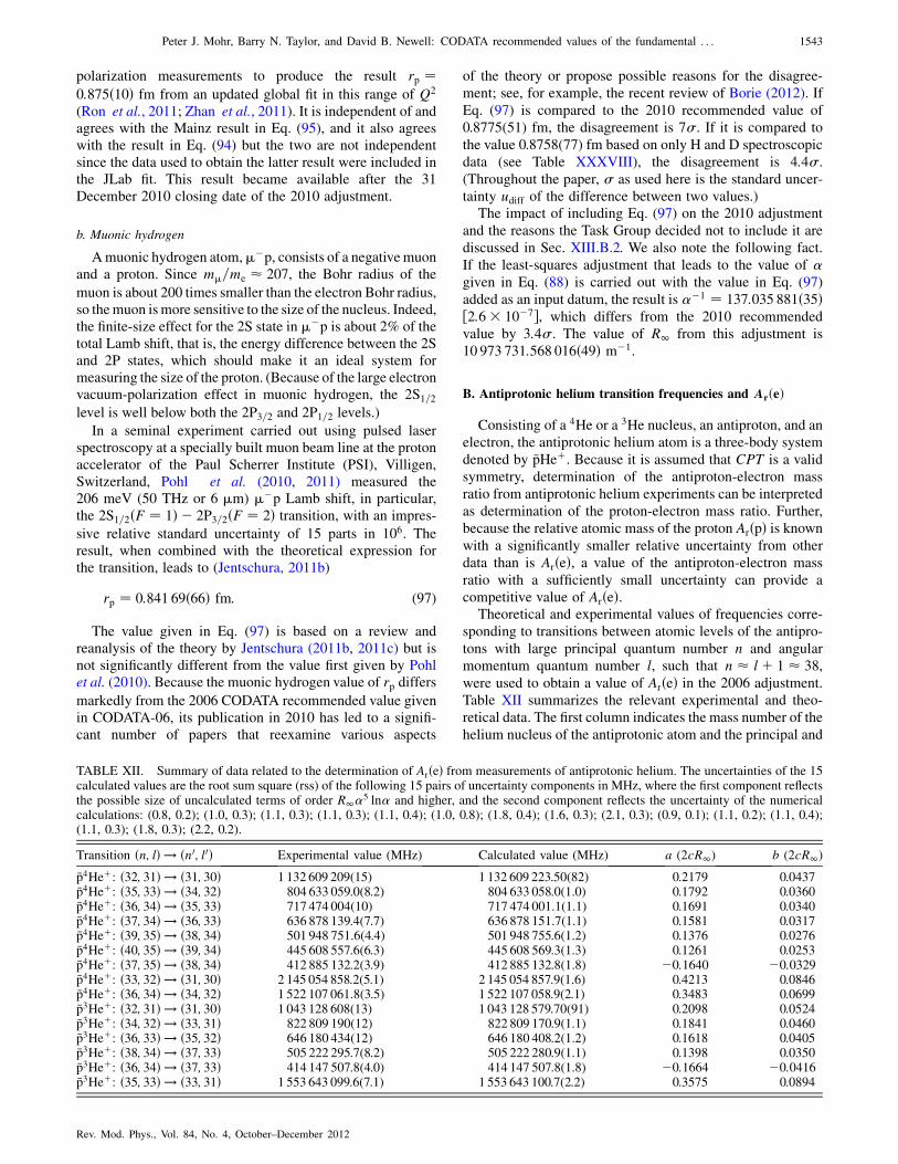
polarization measurements to produce the result rp ¼0:875ð10Þ fm from an updated global fit in this range of Q2
(Ron et al., 2011; Zhan et al., 2011). It is independent of andagrees with the Mainz result in Eq. (95), and it also agreeswith the result in Eq. (94) but the two are not independentsince the data used to obtain the latter result were included inthe JLab fit. This result became available after the 31December 2010 closing date of the 2010 adjustment.
b. Muonic hydrogen
Amuonic hydrogen atom,��p, consists of a negativemuonand a proton. Since m�=me � 207, the Bohr radius of the
muon is about 200 times smaller than the electron Bohr radius,so themuon ismore sensitive to the size of the nucleus. Indeed,the finite-size effect for the 2S state in ��p is about 2% of thetotal Lamb shift, that is, the energy difference between the 2Sand 2P states, which should make it an ideal system formeasuring the size of the proton. (Because of the large electronvacuum-polarization effect in muonic hydrogen, the 2S1=2level is well below both the 2P3=2 and 2P1=2 levels.)
In a seminal experiment carried out using pulsed laserspectroscopy at a specially built muon beam line at the protonaccelerator of the Paul Scherrer Institute (PSI), Villigen,Switzerland, Pohl et al. (2010, 2011) measured the206 meV (50 THz or 6 �m) ��p Lamb shift, in particular,the 2S1=2ðF ¼ 1Þ � 2P3=2ðF ¼ 2Þ transition, with an impres-
sive relative standard uncertainty of 15 parts in 106. Theresult, when combined with the theoretical expression forthe transition, leads to (Jentschura, 2011b)
rp ¼ 0:841 69ð66Þ fm: (97)
The value given in Eq. (97) is based on a review andreanalysis of the theory by Jentschura (2011b, 2011c) but isnot significantly different from the value first given by Pohlet al. (2010). Because the muonic hydrogen value of rp differs
markedly from the 2006 CODATA recommended value givenin CODATA-06, its publication in 2010 has led to a signifi-cant number of papers that reexamine various aspects
of the theory or propose possible reasons for the disagree-
ment; see, for example, the recent review of Borie (2012). If
Eq. (97) is compared to the 2010 recommended value of
0.8775(51) fm, the disagreement is 7�. If it is compared to
the value 0.8758(77) fm based on only H and D spectroscopic
data (see Table XXXVIII), the disagreement is 4:4�.(Throughout the paper, � as used here is the standard uncer-
tainty udiff of the difference between two values.)The impact of including Eq. (97) on the 2010 adjustment
and the reasons the Task Group decided not to include it are
discussed in Sec. XIII.B.2. We also note the following fact.
If the least-squares adjustment that leads to the value of �given in Eq. (88) is carried out with the value in Eq. (97)
added as an input datum, the result is ��1 ¼ 137:035 881ð35Þ½2:6� 10�7�, which differs from the 2010 recommended
value by 3:4�. The value of R1 from this adjustment is
10 973 731:568 016ð49Þ m�1.
B. Antiprotonic helium transition frequencies and ArðeÞ
Consisting of a 4He or a 3He nucleus, an antiproton, and anelectron, the antiprotonic helium atom is a three-body system
denoted by �pHeþ. Because it is assumed that CPT is a valid
symmetry, determination of the antiproton-electron mass
ratio from antiprotonic helium experiments can be interpreted
as determination of the proton-electron mass ratio. Further,
because the relative atomic mass of the proton ArðpÞ is knownwith a significantly smaller relative uncertainty from other
data than is ArðeÞ, a value of the antiproton-electron mass
ratio with a sufficiently small uncertainty can provide a
competitive value of ArðeÞ.Theoretical and experimental values of frequencies corre-
sponding to transitions between atomic levels of the antipro-
tons with large principal quantum number n and angular
momentum quantum number l, such that n � lþ 1 � 38,were used to obtain a value of ArðeÞ in the 2006 adjustment.
Table XII summarizes the relevant experimental and theo-
retical data. The first column indicates the mass number of the
helium nucleus of the antiprotonic atom and the principal and
TABLE XII. Summary of data related to the determination of ArðeÞ from measurements of antiprotonic helium. The uncertainties of the 15calculated values are the root sum square (rss) of the following 15 pairs of uncertainty components in MHz, where the first component reflectsthe possible size of uncalculated terms of order R1�5 ln� and higher, and the second component reflects the uncertainty of the numericalcalculations: (0.8, 0.2); (1.0, 0.3); (1.1, 0.3); (1.1, 0.3); (1.1, 0.4); (1.0, 0.8); (1.8, 0.4); (1.6, 0.3); (2.1, 0.3); (0.9, 0.1); (1.1, 0.2); (1.1, 0.4);(1.1, 0.3); (1.8, 0.3); (2.2, 0.2).
Transition ðn; lÞ ! ðn0; l0Þ Experimental value (MHz) Calculated value (MHz) a (2cR1) b (2cR1)
�p4Heþ: ð32; 31Þ ! ð31; 30Þ 1 132 609 209(15) 1 132 609 223.50(82) 0.2179 0.0437�p4Heþ: ð35; 33Þ ! ð34; 32Þ 804 633 059.0(8.2) 804 633 058.0(1.0) 0.1792 0.0360�p4Heþ: ð36; 34Þ ! ð35; 33Þ 717 474 004(10) 717 474 001.1(1.1) 0.1691 0.0340�p4Heþ: ð37; 34Þ ! ð36; 33Þ 636 878 139.4(7.7) 636 878 151.7(1.1) 0.1581 0.0317�p4Heþ: ð39; 35Þ ! ð38; 34Þ 501 948 751.6(4.4) 501 948 755.6(1.2) 0.1376 0.0276�p4Heþ: ð40; 35Þ ! ð39; 34Þ 445 608 557.6(6.3) 445 608 569.3(1.3) 0.1261 0.0253�p4Heþ: ð37; 35Þ ! ð38; 34Þ 412 885 132.2(3.9) 412 885 132.8(1.8) �0:1640 �0:0329�p4Heþ: ð33; 32Þ ! ð31; 30Þ 2 145 054 858.2(5.1) 2 145 054 857.9(1.6) 0.4213 0.0846�p4Heþ: ð36; 34Þ ! ð34; 32Þ 1 522 107 061.8(3.5) 1 522 107 058.9(2.1) 0.3483 0.0699�p3Heþ: ð32; 31Þ ! ð31; 30Þ 1 043 128 608(13) 1 043 128 579.70(91) 0.2098 0.0524�p3Heþ: ð34; 32Þ ! ð33; 31Þ 822 809 190(12) 822 809 170.9(1.1) 0.1841 0.0460�p3Heþ: ð36; 33Þ ! ð35; 32Þ 646 180 434(12) 646 180 408.2(1.2) 0.1618 0.0405�p3Heþ: ð38; 34Þ ! ð37; 33Þ 505 222 295.7(8.2) 505 222 280.9(1.1) 0.1398 0.0350�p3Heþ: ð36; 34Þ ! ð37; 33Þ 414 147 507.8(4.0) 414 147 507.8(1.8) �0:1664 �0:0416�p3Heþ: ð35; 33Þ ! ð33; 31Þ 1 553 643 099.6(7.1) 1 553 643 100.7(2.2) 0.3575 0.0894
Peter J. Mohr, Barry N. Taylor, and David B. Newell: CODATA recommended values of the fundamental . . . 1543
Rev. Mod. Phys., Vol. 84, No. 4, October–December 2012
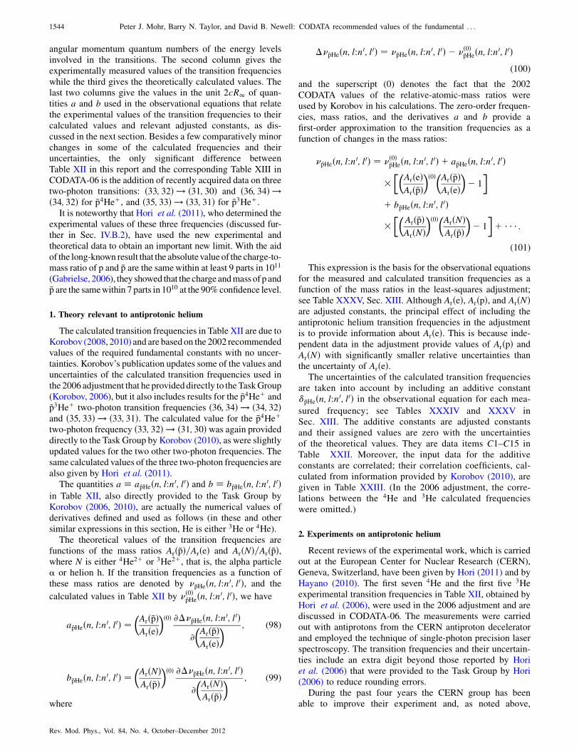
angular momentum quantum numbers of the energy levelsinvolved in the transitions. The second column gives theexperimentally measured values of the transition frequencieswhile the third gives the theoretically calculated values. Thelast two columns give the values in the unit 2cR1 of quan-tities a and b used in the observational equations that relatethe experimental values of the transition frequencies to theircalculated values and relevant adjusted constants, as dis-cussed in the next section. Besides a few comparatively minorchanges in some of the calculated frequencies and theiruncertainties, the only significant difference betweenTable XII in this report and the corresponding Table XIII inCODATA-06 is the addition of recently acquired data on threetwo-photon transitions: ð33; 32Þ ! ð31; 30Þ and ð36; 34Þ !ð34; 32Þ for �p4Heþ, and ð35; 33Þ ! ð33; 31Þ for �p3Heþ.
It is noteworthy that Hori et al. (2011), who determined theexperimental values of these three frequencies (discussed fur-ther in Sec. IV.B.2), have used the new experimental andtheoretical data to obtain an important new limit. With the aidof the long-known result that the absolutevalue of the charge-to-mass ratio of p and �p are the samewithin at least 9 parts in 1011
(Gabrielse, 2006), they showed that the charge andmass ofp and�p are the samewithin 7 parts in 1010 at the 90%confidence level.
1. Theory relevant to antiprotonic helium
The calculated transition frequencies in Table XII are due toKorobov (2008, 2010) and are based on the 2002 recommendedvalues of the required fundamental constants with no uncer-tainties. Korobov’s publication updates some of the values anduncertainties of the calculated transition frequencies used inthe 2006 adjustment that he provideddirectly to theTaskGroup(Korobov, 2006), but it also includes results for the �p4Heþ and�p3Heþ two-photon transition frequencies ð36; 34Þ ! ð34; 32Þand ð35; 33Þ ! ð33; 31Þ. The calculated value for the �p4Heþtwo-photon frequency ð33; 32Þ ! ð31; 30Þ was again provideddirectly to the Task Group by Korobov (2010), as were slightlyupdated values for the two other two-photon frequencies. Thesame calculated values of the three two-photon frequencies arealso given by Hori et al. (2011).
The quantities a � a�pHeðn; l:n0; l0Þ and b � b�pHeðn; l:n0; l0Þin Table XII, also directly provided to the Task Group byKorobov (2006, 2010), are actually the numerical values ofderivatives defined and used as follows (in these and othersimilar expressions in this section, He is either 3He or 4He).
The theoretical values of the transition frequencies arefunctions of the mass ratios Arð�pÞ=ArðeÞ and ArðNÞ=Arð�pÞ,where N is either 4He2þ or 3He2þ, that is, the alpha particle� or helion h. If the transition frequencies as a function ofthese mass ratios are denoted by ��pHeðn; l:n0; l0Þ, and the
calculated values in Table XII by �ð0Þ�pHeðn; l:n0; l0Þ, we have
a�pHeðn; l:n0; l0Þ ¼�Arð�pÞArðeÞ
�ð0Þ @���pHeðn; l:n0; l0Þ@
�Arð�pÞArðeÞ
� ; (98)
b�pHeðn; l:n0; l0Þ ¼�ArðNÞArð�pÞ
�ð0Þ @���pHeðn; l:n0; l0Þ@
�ArðNÞArð�pÞ
� ; (99)
where
���pHeðn; l:n0; l0Þ ¼ ��pHeðn; l:n0; l0Þ � �ð0Þ�pHeðn; l:n0; l0Þ
(100)
and the superscript (0) denotes the fact that the 2002CODATA values of the relative-atomic-mass ratios wereused by Korobov in his calculations. The zero-order frequen-cies, mass ratios, and the derivatives a and b provide afirst-order approximation to the transition frequencies as afunction of changes in the mass ratios:
��pHeðn; l:n0; l0Þ ¼ �ð0Þ�pHeðn; l:n0; l0Þ þ a�pHeðn; l:n0; l0Þ
���
ArðeÞArð�pÞ
�ð0Þ�Arð�pÞArðeÞ
�� 1
�
þ b�pHeðn; l:n0; l0Þ
���
Arð�pÞArðNÞ
�ð0Þ�ArðNÞArð�pÞ
�� 1
�þ � � � :
(101)
This expression is the basis for the observational equationsfor the measured and calculated transition frequencies as afunction of the mass ratios in the least-squares adjustment;see Table XXXV, Sec. XIII. Although ArðeÞ, ArðpÞ, and ArðNÞare adjusted constants, the principal effect of including theantiprotonic helium transition frequencies in the adjustmentis to provide information about ArðeÞ. This is because inde-pendent data in the adjustment provide values of ArðpÞ andArðNÞ with significantly smaller relative uncertainties thanthe uncertainty of ArðeÞ.
The uncertainties of the calculated transition frequenciesare taken into account by including an additive constant��pHeðn; l:n0; l0Þ in the observational equation for each mea-
sured frequency; see Tables XXXIV and XXXV inSec. XIII. The additive constants are adjusted constantsand their assigned values are zero with the uncertaintiesof the theoretical values. They are data items C1–C15 inTable XXII. Moreover, the input data for the additiveconstants are correlated; their correlation coefficients, cal-culated from information provided by Korobov (2010), aregiven in Table XXIII. (In the 2006 adjustment, the corre-lations between the 4He and 3He calculated frequencieswere omitted.)
2. Experiments on antiprotonic helium
Recent reviews of the experimental work, which is carriedout at the European Center for Nuclear Research (CERN),Geneva, Switzerland, have been given by Hori (2011) and byHayano (2010). The first seven 4He and the first five 3Heexperimental transition frequencies in Table XII, obtained byHori et al. (2006), were used in the 2006 adjustment and arediscussed in CODATA-06. The measurements were carriedout with antiprotons from the CERN antiproton deceleratorand employed the technique of single-photon precision laserspectroscopy. The transition frequencies and their uncertain-ties include an extra digit beyond those reported by Horiet al. (2006) that were provided to the Task Group by Hori(2006) to reduce rounding errors.
During the past four years the CERN group has beenable to improve their experiment and, as noted above,
1544 Peter J. Mohr, Barry N. Taylor, and David B. Newell: CODATA recommended values of the fundamental . . .
Rev. Mod. Phys., Vol. 84, No. 4, October–December 2012
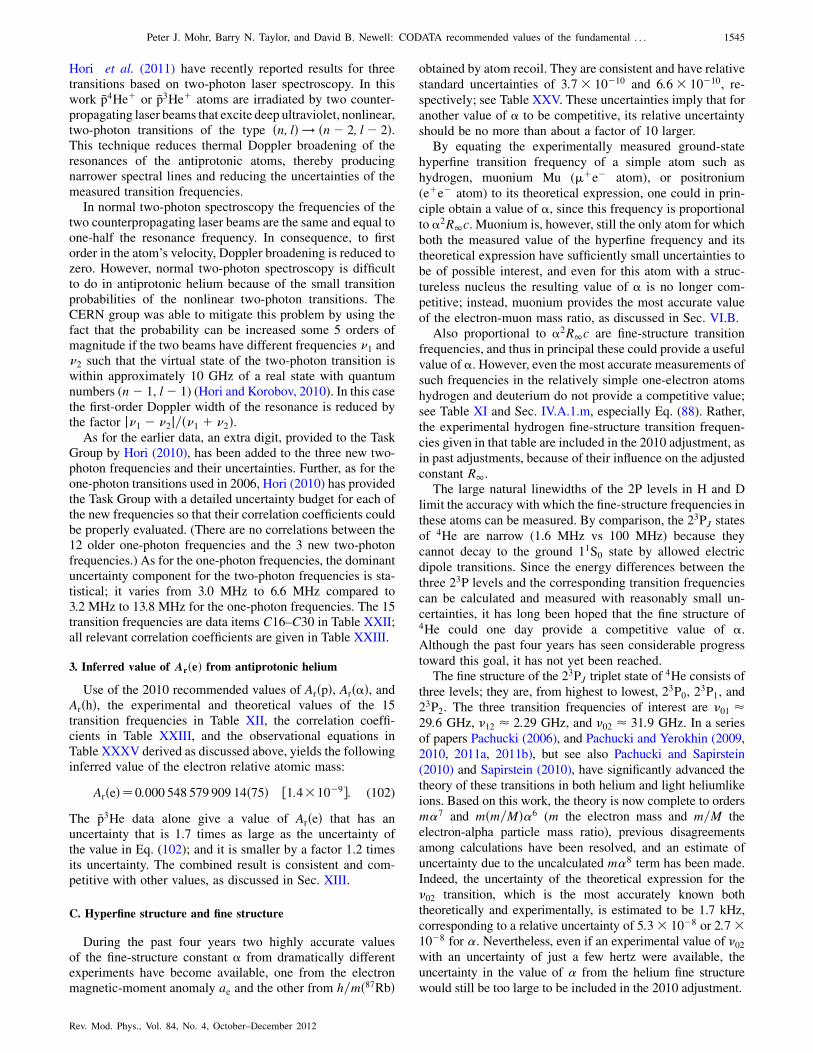
Hori et al. (2011) have recently reported results for threetransitions based on two-photon laser spectroscopy. In thiswork �p4Heþ or �p3Heþ atoms are irradiated by two counter-propagating laser beams that excite deep ultraviolet, nonlinear,two-photon transitions of the type ðn; lÞ ! ðn� 2; l� 2Þ.This technique reduces thermal Doppler broadening of theresonances of the antiprotonic atoms, thereby producingnarrower spectral lines and reducing the uncertainties of themeasured transition frequencies.
In normal two-photon spectroscopy the frequencies of thetwo counterpropagating laser beams are the same and equal toone-half the resonance frequency. In consequence, to firstorder in the atom’s velocity, Doppler broadening is reduced tozero. However, normal two-photon spectroscopy is difficultto do in antiprotonic helium because of the small transitionprobabilities of the nonlinear two-photon transitions. TheCERN group was able to mitigate this problem by using thefact that the probability can be increased some 5 orders ofmagnitude if the two beams have different frequencies �1 and�2 such that the virtual state of the two-photon transition iswithin approximately 10 GHz of a real state with quantumnumbers (n� 1, l� 1) (Hori and Korobov, 2010). In this casethe first-order Doppler width of the resonance is reduced bythe factor j�1 � �2j=ð�1 þ �2Þ.
As for the earlier data, an extra digit, provided to the TaskGroup by Hori (2010), has been added to the three new two-photon frequencies and their uncertainties. Further, as for theone-photon transitions used in 2006, Hori (2010) has providedthe Task Group with a detailed uncertainty budget for each ofthe new frequencies so that their correlation coefficients couldbe properly evaluated. (There are no correlations between the12 older one-photon frequencies and the 3 new two-photonfrequencies.) As for the one-photon frequencies, the dominantuncertainty component for the two-photon frequencies is sta-tistical; it varies from 3.0 MHz to 6.6 MHz compared to3.2 MHz to 13.8 MHz for the one-photon frequencies. The 15transition frequencies are data items C16–C30 in Table XXII;all relevant correlation coefficients are given in Table XXIII.
3. Inferred value of ArðeÞ from antiprotonic helium
Use of the 2010 recommended values of ArðpÞ, Arð�Þ, andArðhÞ, the experimental and theoretical values of the 15transition frequencies in Table XII, the correlation coeffi-cients in Table XXIII, and the observational equations inTable XXXV derived as discussed above, yields the followinginferred value of the electron relative atomic mass:
ArðeÞ¼0:000 548 579 909 14ð75Þ ½1:4�10�9�: (102)
The �p3He data alone give a value of ArðeÞ that has anuncertainty that is 1.7 times as large as the uncertainty ofthe value in Eq. (102); and it is smaller by a factor 1.2 timesits uncertainty. The combined result is consistent and com-petitive with other values, as discussed in Sec. XIII.
C. Hyperfine structure and fine structure
During the past four years two highly accurate valuesof the fine-structure constant � from dramatically differentexperiments have become available, one from the electronmagnetic-moment anomaly ae and the other from h=mð87RbÞ
obtained by atom recoil. They are consistent and have relative
standard uncertainties of 3:7� 10�10 and 6:6� 10�10, re-
spectively; see Table XXV. These uncertainties imply that for
another value of � to be competitive, its relative uncertainty
should be no more than about a factor of 10 larger.By equating the experimentally measured ground-state
hyperfine transition frequency of a simple atom such as
hydrogen, muonium Mu (�þe� atom), or positronium
(eþe� atom) to its theoretical expression, one could in prin-
ciple obtain a value of �, since this frequency is proportional
to �2R1c. Muonium is, however, still the only atom for which
both the measured value of the hyperfine frequency and its
theoretical expression have sufficiently small uncertainties to
be of possible interest, and even for this atom with a struc-
tureless nucleus the resulting value of � is no longer com-
petitive; instead, muonium provides the most accurate value
of the electron-muon mass ratio, as discussed in Sec. VI.B.Also proportional to �2R1c are fine-structure transition
frequencies, and thus in principal these could provide a useful
value of �. However, even the most accurate measurements of
such frequencies in the relatively simple one-electron atoms
hydrogen and deuterium do not provide a competitive value;
see Table XI and Sec. IV.A.1.m, especially Eq. (88). Rather,
the experimental hydrogen fine-structure transition frequen-
cies given in that table are included in the 2010 adjustment, as
in past adjustments, because of their influence on the adjusted
constant R1.The large natural linewidths of the 2P levels in H and D
limit the accuracy with which the fine-structure frequencies in
these atoms can be measured. By comparison, the 23PJ statesof 4He are narrow (1.6 MHz vs 100 MHz) because they
cannot decay to the ground 11S0 state by allowed electric
dipole transitions. Since the energy differences between the
three 23P levels and the corresponding transition frequencies
can be calculated and measured with reasonably small un-
certainties, it has long been hoped that the fine structure of4He could one day provide a competitive value of �.Although the past four years has seen considerable progress
toward this goal, it has not yet been reached.The fine structure of the 23PJ triplet state of
4He consists ofthree levels; they are, from highest to lowest, 23P0, 2
3P1, and23P2. The three transition frequencies of interest are �01 �29:6 GHz, �12 � 2:29 GHz, and �02 � 31:9 GHz. In a series
of papers Pachucki (2006), and Pachucki and Yerokhin (2009,
2010, 2011a, 2011b), but see also Pachucki and Sapirstein
(2010) and Sapirstein (2010), have significantly advanced the
theory of these transitions in both helium and light heliumlike
ions. Based on this work, the theory is now complete to orders
m�7 and mðm=MÞ�6 (m the electron mass and m=M the
electron-alpha particle mass ratio), previous disagreements
among calculations have been resolved, and an estimate of
uncertainty due to the uncalculated m�8 term has been made.
Indeed, the uncertainty of the theoretical expression for the
�02 transition, which is the most accurately known both
theoretically and experimentally, is estimated to be 1.7 kHz,
corresponding to a relative uncertainty of 5:3� 10�8 or 2:7�10�8 for �. Nevertheless, even if an experimental value of �02with an uncertainty of just a few hertz were available, the
uncertainty in the value of � from the helium fine structure
would still be too large to be included in the 2010 adjustment.
Peter J. Mohr, Barry N. Taylor, and David B. Newell: CODATA recommended values of the fundamental . . . 1545
Rev. Mod. Phys., Vol. 84, No. 4, October–December 2012
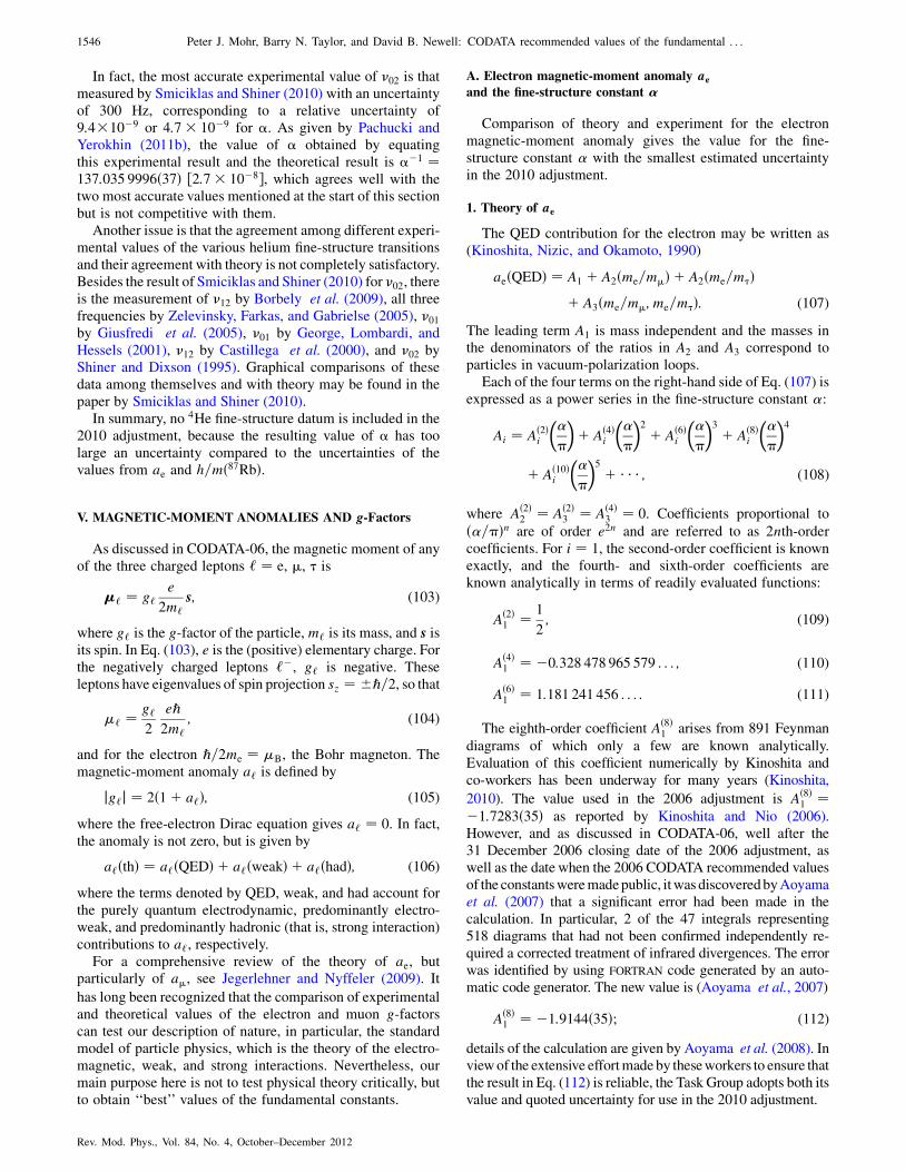
In fact, the most accurate experimental value of �02 is thatmeasured by Smiciklas and Shiner (2010) with an uncertaintyof 300 Hz, corresponding to a relative uncertainty of9:4�10�9 or 4:7� 10�9 for �. As given by Pachucki andYerokhin (2011b), the value of � obtained by equatingthis experimental result and the theoretical result is ��1 ¼137:035 9996ð37Þ ½2:7� 10�8�, which agrees well with thetwo most accurate values mentioned at the start of this sectionbut is not competitive with them.
Another issue is that the agreement among different experi-mental values of the various helium fine-structure transitionsand their agreement with theory is not completely satisfactory.Besides the result of Smiciklas and Shiner (2010) for �02, thereis the measurement of �12 by Borbely et al. (2009), all threefrequencies by Zelevinsky, Farkas, and Gabrielse (2005), �01by Giusfredi et al. (2005), �01 by George, Lombardi, andHessels (2001), �12 by Castillega et al. (2000), and �02 byShiner and Dixson (1995). Graphical comparisons of thesedata among themselves and with theory may be found in thepaper by Smiciklas and Shiner (2010).
In summary, no 4He fine-structure datum is included in the2010 adjustment, because the resulting value of � has toolarge an uncertainty compared to the uncertainties of thevalues from ae and h=mð87RbÞ.
V. MAGNETIC-MOMENT ANOMALIES AND g-Factors
As discussed in CODATA-06, the magnetic moment of anyof the three charged leptons ‘ ¼ e, �, � is
�‘ ¼ g‘e
2m‘
s; (103)
where g‘ is the g-factor of the particle,m‘ is its mass, and s isits spin. In Eq. (103), e is the (positive) elementary charge. Forthe negatively charged leptons ‘�, g‘ is negative. Theseleptons have eigenvalues of spin projection sz ¼ ℏ=2, so that
�‘ ¼ g‘2
eℏ2m‘
; (104)
and for the electron ℏ=2me ¼ �B, the Bohr magneton. Themagnetic-moment anomaly a‘ is defined by
jg‘j ¼ 2ð1þ a‘Þ; (105)
where the free-electron Dirac equation gives a‘ ¼ 0. In fact,the anomaly is not zero, but is given by
a‘ðthÞ ¼ a‘ðQEDÞ þ a‘ðweakÞ þ a‘ðhadÞ; (106)
where the terms denoted by QED, weak, and had account forthe purely quantum electrodynamic, predominantly electro-weak, and predominantly hadronic (that is, strong interaction)contributions to a‘, respectively.
For a comprehensive review of the theory of ae, butparticularly of a�, see Jegerlehner and Nyffeler (2009). It
has long been recognized that the comparison of experimentaland theoretical values of the electron and muon g-factorscan test our description of nature, in particular, the standardmodel of particle physics, which is the theory of the electro-magnetic, weak, and strong interactions. Nevertheless, ourmain purpose here is not to test physical theory critically, butto obtain ‘‘best’’ values of the fundamental constants.
A. Electron magnetic-moment anomaly ae
and the fine-structure constant �
Comparison of theory and experiment for the electronmagnetic-moment anomaly gives the value for the fine-structure constant � with the smallest estimated uncertaintyin the 2010 adjustment.
1. Theory of ae
The QED contribution for the electron may be written as(Kinoshita, Nizic, and Okamoto, 1990)
aeðQEDÞ ¼ A1 þ A2ðme=m�Þ þ A2ðme=m�Þþ A3ðme=m�; me=m�Þ: (107)
The leading term A1 is mass independent and the masses inthe denominators of the ratios in A2 and A3 correspond toparticles in vacuum-polarization loops.
Each of the four terms on the right-hand side of Eq. (107) isexpressed as a power series in the fine-structure constant �:
Ai ¼ Að2Þi
��
�
�þ Að4Þ
i
��
�
�2 þ Að6Þ
i
��
�
�3 þ Að8Þ
i
��
�
�4
þ Að10Þi
��
�
�5 þ � � � ; (108)
where Að2Þ2 ¼ Að2Þ
3 ¼ Að4Þ3 ¼ 0. Coefficients proportional to
ð�=�Þn are of order e2n and are referred to as 2nth-ordercoefficients. For i ¼ 1, the second-order coefficient is knownexactly, and the fourth- and sixth-order coefficients areknown analytically in terms of readily evaluated functions:
Að2Þ1 ¼ 1
2; (109)
Að4Þ1 ¼ �0:328 478 965 579 . . . ; (110)
Að6Þ1 ¼ 1:181 241 456 . . . : (111)
The eighth-order coefficient Að8Þ1 arises from 891 Feynman
diagrams of which only a few are known analytically.Evaluation of this coefficient numerically by Kinoshita andco-workers has been underway for many years (Kinoshita,
2010). The value used in the 2006 adjustment is Að8Þ1 ¼
�1:7283ð35Þ as reported by Kinoshita and Nio (2006).However, and as discussed in CODATA-06, well after the31 December 2006 closing date of the 2006 adjustment, aswell as the date when the 2006 CODATA recommended valuesof the constantsweremadepublic, itwas discoveredbyAoyamaet al. (2007) that a significant error had been made in thecalculation. In particular, 2 of the 47 integrals representing518 diagrams that had not been confirmed independently re-quired a corrected treatment of infrared divergences. The errorwas identified by using FORTRAN code generated by an auto-matic code generator. The new value is (Aoyama et al., 2007)
Að8Þ1 ¼ �1:9144ð35Þ; (112)
details of the calculation are given by Aoyama et al. (2008). Inviewof the extensive effortmadeby theseworkers to ensure thatthe result in Eq. (112) is reliable, the Task Group adopts both itsvalue and quoted uncertainty for use in the 2010 adjustment.
1546 Peter J. Mohr, Barry N. Taylor, and David B. Newell: CODATA recommended values of the fundamental . . .
Rev. Mod. Phys., Vol. 84, No. 4, October–December 2012
Independent work is in progress on analytic calculations ofeighth-order integrals; see, for example, Laporta (2001,2008), Mastrolia and Remiddi (2001), and Laporta,Mastrolia, and Remiddi (2004). Work is also in progress onnumerical calculations of the 12 672 Feynman diagrams forthe tenth-order coefficient; see Aoyama et al. (2011) andreferences cited therein.
The evaluationof the contribution to the uncertainty ofaeðthÞfrom the fact that Að10Þ
1 is unknown follows the procedure in
CODATA-98 and yields Að10Þ1 ¼ 0:0ð4:6Þ, which contributes a
standard uncertainty component to aeðthÞ of 2:7� 10�10ae.
This uncertainty is larger than the uncertainty attributed toAð10Þ1
in CODATA-06, because the absolute value of Að8Þ1 has in-
creased. All higher-order coefficients are assumed to benegligible.
The mass-dependent coefficients for the electron based onthe 2010 recommended values of the mass ratios are
Að4Þ2 ðme=m�Þ ¼ 5:197 386 68ð26Þ � 10�7
! 24:182� 10�10ae; (113)
Að4Þ2 ðme=m�Þ ¼ 1:837 98ð33Þ � 10�9
! 0:086� 10�10ae; (114)
Að6Þ2 ðme=m�Þ ¼ �7:373 941 62ð27Þ � 10�6
! �0:797� 10�10ae; (115)
Að6Þ2 ðme=m�Þ ¼ �6:5830ð11Þ � 10�8
! �0:007� 10�10ae; (116)
where the standard uncertainties of the coefficients are due tothe uncertainties of the mass ratios and are negligible. The
contributions from Að6Þ3 ðme=m�; me=m�Þ and all higher-order
mass-dependent terms are also negligible.Thedependenceon� ofany contributionother thanaeðQEDÞ
is negligible, hence the anomaly as a function of � is given bycombining QED terms that have like powers of �=�:
aeðQEDÞ ¼ Cð2Þe
��
�
�þ Cð4Þ
e
��
�
�2 þ Cð6Þ
e
��
�
�3
þ Cð8Þe
��
�
�4 þ Cð10Þ
e
��
�
�5 þ � � � ; (117)
with
Cð2Þe ¼ 0:5;
Cð4Þe ¼ �0:328 478 444 00;
Cð6Þe ¼ 1:181 234 017;
Cð8Þe ¼ �1:9144ð35Þ;
Cð10Þe ¼ 0:0ð4:6Þ:
(118)
The electroweak contribution, calculated as in CODATA-98 but with the 2010 values of GF and sin2�W, is
aeðweakÞ ¼ 0:029 73ð52Þ � 10�12
¼ 0:2564ð45Þ � 10�10ae: (119)
The hadronic contribution can be written as
aeðhadÞ ¼ að4Þe ðhadÞ þ að6aÞe ðhadÞ þ að��Þe ðhadÞ þ � � � ;(120)
where að4Þe ðhadÞ and að6aÞe ðhadÞ are due to hadronic vacuumpolarization and are of order ð�=�Þ2 and ð�=�Þ3, respec-tively; also of order ð�=�Þ3 is að��Þ� , which is due to light-by-light vacuum polarization. The total value
aeðhadÞ ¼ 1:685ð22Þ � 10�12
¼ 1:453ð19Þ � 10�9ae (121)
is the sum of the following three contributions: að4Þe ðhadÞ ¼1:875ð18Þ � 10�12 obtained by Davier and Hocker (1998);
að6aÞe ðhadÞ¼�0:225ð5Þ�10�12 given by Krause (1997); and
að��Þe ðhadÞ¼0:035ð10Þ�10�12 as given by Prades, de Rafael,and Vainshtein (2010). In past adjustments this contribution
was calculated by assuming that að��Þe ¼ðme=m�Þ2að��Þ� ðhadÞ.However, Prades, de Rafael, and Vainshtein (2010) haveshown that such scaling is not adequate for the neutral pion
exchange contribution to að��Þ� ðhadÞ and have taken this into
account in obtaining their above result for að��Þe ðhadÞ from
their muon value að��Þ� ðhadÞ ¼ 105ð26Þ � 10�11.The theoretical prediction is
aeðthÞ ¼ aeðQEDÞ þ aeðweakÞ þ aeðhadÞ: (122)
Thevarious contributions can be put into context by comparingthem to the most accurate experimental value of ae currentlyavailable, which has an uncertainty of 2:8� 10�10ae; seeEq. (126).
The standard uncertainty of aeðthÞ from the uncertainties ofthe terms listed above is
u½aeðthÞ� ¼ 0:33� 10�12 ¼ 2:8� 10�10ae (123)
and is dominated by the uncertainty of the coefficient Cð10Þe .
For the purpose of the least-squares calculations carriedout in Sec. XIII, we include an additive correction �e to aeðthÞto account for the uncertainty of aeðthÞ other than that due to�, and hence the complete theoretical expression in theobservational equation for the electron anomaly (B13 inTable XXXIII) is
aeð�; �eÞ ¼ aeðthÞ þ �e: (124)
The input datum for �e is zero with standard uncertaintyu½aeðthÞ�, or 0:00ð33Þ�10�12, which is data item B12 inTable XX.
2. Measurements of ae
a. University of Washington
The classic series of measurements of the electron andpositron anomalies carried out at the University ofWashington by Van Dyck, Jr., Schwinberg, and Dehmelt(1987) yield the value
ae¼1:159 652 1883ð42Þ�10�3 ½3:7�10�9�; (125)
as discussed in CODATA-98. This result, which assumes thatCPT invariance holds for the electron-positron system, is dataitem B13:1 in Table XX.
b. Harvard University
In both the University of Washington and HarvardUniversity, Cambridge, MA, USA experiments, the electron
Peter J. Mohr, Barry N. Taylor, and David B. Newell: CODATA recommended values of the fundamental . . . 1547
Rev. Mod. Phys., Vol. 84, No. 4, October–December 2012
magnetic-moment anomaly is essentially determined fromthe relation ae ¼ fa=fc by measuring in the same magneticflux density B � 5 T the anomaly difference frequency fa ¼fs � fc and cyclotron frequency fc ¼ eB=2�me, where fs ¼jgej�BB=h is the electron spin-flip (or precession) frequency.
Because of its small relative standard uncertainty of 7:6�10�10, the then new result for ae obtained by Odom et al.(2006) at Harvard using a cylindrical rather than a hyperbolicPenning trap played the dominant role in determining the2006 recommended value of �. This work continued with anumber of significant improvements and a new value of aeconsistent with the earlier one but with an uncertainty nearlya factor of 3 smaller was reported by Hanneke, Fogwell, andGabrielse (2008):
ae ¼ 1:159 652 180 73ð28Þ � 10�3: (126)
A paper that describes this measurement in detail was sub-sequently published by Hanneke, Fogwell Hoogerheide, andGabrielse (2011) [see also the review by Gabrielse (2010)].As discussed by Hanneke, Fogwell Hoogerheide, andGabrielse (2011), the improvement that contributed most tothe reduction in uncertainty is a better understanding of thePenning-trap cavity frequency shifts of the radiation used tomeasure fc. A smaller reduction resulted from narrowerlinewidths of the anomaly and cyclotron resonant frequen-cies. Consequently, Hanneke, Fogwell Hoogerheide, andGabrielse (2011) state that their 2008 result should be viewedas superseding the earlier Harvard result. Therefore, only thevalue of ae in Eq. (126) is included as an input datum in the2010 adjustment; it is data item B13:2 in Table XX.
3. Values of � inferred from ae
Equating the theoretical expression with the two experi-mental values of ae given in Eqs. (125) and (126) yields
��1ðaeÞ¼137:03599819ð50Þ ½3:7�10�9� (127)
from the University of Washington result and
��1ðaeÞ¼137:035999084ð51Þ ½3:7�10�10� (128)
from the Harvard University result. The contribution of theuncertainty in aeðthÞ to the relative uncertainty of either ofthese results is 2:8� 10�10. The value in Eq. (128) has thesmallest uncertainty of any value of alpha currently available.The fact that the next most accurate value of �, which has arelative standard uncertainty of 6:6� 10�10 and is obtainedfrom the quotient h=mð87RbÞ measured by atom recoil, isconsistent with this value suggests that the theory of ae is wellin hand; see Sec. XIII.
B. Muon magnetic-moment anomaly a�
The 2006 adjustment included data that provided both anexperimental value and a theoretical value for a�. Because of
problems with the theory, the uncertainty assigned to thetheoretical value was over 3 times larger than that of theexperimental value. Nevertheless, the theoretical value withits increased uncertainty was included in the adjustment, evenif with a comparatively small weight.
For the 2010 adjustment, the Task Group decided not toinclude the theoretical value for a�, with the result that the
2010 recommended value is based mainly on experiment.This is consistent with the fact that the value of a� recom-
mended by the Particle Data Group in their biennial 2010Review of Particle Physics (Nakamura et al., 2010) is theexperimental value. The current situation is briefly summa-rized in the following sections.
1. Theory of a�
Themass-independent coefficients AðnÞ1 for the muon are the
same as for the electron. Based on the 2010 recommendedvalues of the mass ratios, the relevant mass-dependent termsare
Að4Þ2 ðm�=meÞ ¼ 1:094 258 3118ð81Þ
! 506 386:4620ð38Þ � 10�8a�; (129)
Að4Þ2 ðm�=m�Þ ¼ 0:000 078 079ð14Þ
! 36:1325ð65Þ � 10�8a�; (130)
Að6Þ2 ðm�=meÞ ¼ 22:868 380 04ð19Þ
! 24 581:766 56ð20Þ � 10�8a�; (131)
Að6Þ2 ðm�=m�Þ ¼ 0:000 360 63ð11Þ
! 0:387 65ð12Þ � 10�8a�; (132)
Að8Þ2 ðm�=meÞ ¼ 132:6823ð72Þ
! 331:288ð18Þ � 10�8a�; (133)
Að10Þ2 ðm�=meÞ ¼ 663ð20Þ
! 3:85ð12Þ � 10�8a�; (134)
Að6Þ3 ðm�=me; m�=m�Þ ¼ 0:000 527 762ð94Þ
! 0:567 30ð10Þ � 10�8a�; (135)
Að8Þ3 ðm�=me;m�=m�Þ¼0:037594ð83Þ
!0:09387ð21Þ�10�8a�: (136)
The QED contribution to the theory of a�, where terms that
have like powers of �=� are combined, is
a�ðQEDÞ ¼ Cð2Þ�
��
�
�þ Cð4Þ
�
��
�
�2 þ Cð6Þ
�
��
�
�3
þ Cð8Þ�
��
�
�4 þ Cð10Þ
�
��
�
�5 þ � � � ; (137)
with
Cð2Þ� ¼ 0:5;
Cð4Þ� ¼ 0:765 857 426ð16Þ;
Cð6Þ� ¼ 24:050 509 88ð28Þ;
Cð8Þ� ¼ 130:8055ð80Þ;
Cð10Þ� ¼ 663ð21Þ;
(138)
which yields, using the 2010 recommended value of �,
a�ðQEDÞ ¼ 0:001 165 847 1810ð15Þ ½1:3� 10�9�:(139)
1548 Peter J. Mohr, Barry N. Taylor, and David B. Newell: CODATA recommended values of the fundamental . . .
Rev. Mod. Phys., Vol. 84, No. 4, October–December 2012
In absolute terms, the uncertainty in a�ðQEDÞ is
0:15� 10�11.The current theoretical expression for the muon anomaly is
of the same form as for the electron:
a�ðthÞ ¼ a�ðQEDÞ þ a�ðweakÞ þ a�ðhadÞ: (140)
The electroweak contribution, calculated by Czarnecki et al.(2003), is a�ðweakÞ ¼ 154ð2Þ � 10�11. In contrast to the case
of the electron, a�ðweakÞ is a significant contribution com-
pared to a�ðQEDÞ.In a manner similar to that for the electron, the hadronic
contribution can be written as
a�ðhadÞ ¼ að4Þ� ðhadÞ þ að6aÞ� ðhadÞ þ að��Þ� ðhadÞ þ � � � :(141)
It is also of much greater importance for the muon than for theelectron. Indeed, a�ðhadÞ is roughly 7000ð50Þ � 10�11, which
should be compared with the 63� 10�11 uncertainty of theexperimental value a�ðexpÞ discussed in the next section.
For well over a decade a great deal of effort has beendevoted by many researchers to the improved evaluation of
a�ðhadÞ. The standard method of calculating að4Þ� ðhadÞ and
að6aÞ� ðhadÞ is to evaluate dispersion integrals over experimen-tally measured cross sections for the scattering of eþe� intohadrons. However, in some calculations data on decays of the� into hadrons are used to replace the eþe� data in certainenergy regions. The results of three evaluations which includethe most recent data can be concisely summarized as follows.
Davier et al. (2011) find that a�ðexpÞ exceeds their
theoretically predicted value a�ðthÞ by 3.6 times the com-
bined standard uncertainty of the difference, or 3:6�, usingonly eþe� data, and by 2:4� if � data are included. On theother hand, Jegerlehner and Szafron (2011) find that bycorrecting the � data for the effect they term �-� mixing,
the values of að4Þ� ðhadÞ obtained from only eþe� data, andfrom eþe� and � data together, are nearly identical and thatthe difference between experiment and theory is 3:3�. AndHagiwara et al. (2011) find the same 3:3� difference usingeþe� data alone. Finally, we note that in a very recent paper,Benayoun et al. (2012) obtain a difference in the range4:07� to 4:65�, depending on the assumptions made, usinga ‘‘hidden local symmetry’’ model.
The disagreement between experiment and theory has longbeen known and numerous theoretical papers have been pub-lished that attempt to explain the discrepancy in terms of newphysics; see Stockinger (2010). Although a contribution toa�ðthÞ large enough to bring it into agreement with a�ðexpÞfromphysics beyond the standardmodel is possible, no outsideexperimental evidence currently exists for such physics. Thus,because of the persistence of the discrepancy and its confirma-tion by the most recent calculations, and because no knownphysics has yet been able to eliminate it, the Task Group hasdecided to omit the theory of a� from the 2010 adjustment.
2. Measurement of a�: Brookhaven
Experiment E821 at Brookhaven National Laboratory(BNL), Upton, New York, USA, has been discussed in thepast three CODATA reports. It involves the direct measurement
of the anomaly difference frequency fa ¼ fs � fc, wherefs ¼ jg�jðeℏ=2m�ÞB=h is the muon spin-flip (or precession)
frequency in the applied magnetic flux density B andfc ¼ eB=2�m� is the corresponding muon cyclotron fre-
quency. However, in contrast to the case of the electron whereboth fa and fc are measured directly and the electronanomaly is calculated from ae ¼ fa=fc, for the muon B iseliminated by determining its value from proton nuclearmagnetic resonance (NMR) measurements. This means thatthe muon anomaly is calculated from
a�ðexpÞ ¼�R
j��=�pj � �R; (142)
where �R ¼ fa= �fp and �fp is the free proton NMR frequency
corresponding to the average flux density B seen by themuons in their orbits in the muon storage ring.
The final value of �R obtained in the E821 experiment is(Bennett et al., 2006)
�R ¼ 0:003 707 2063ð20Þ; (143)
which is used as an input datum in the 2010 adjustment and isdata item B14 in Table XX. [The last digit of this value is 1less than that of the value used in 2006, because the 2006value was taken from Eq. (57) in the paper by Bennett et al.(2006) but the correct value is that given in Table XV(Roberts, 2009).] Based on this value of �R, Eq. (142), andthe 2010 recommended value of��=�p, whose uncertainty is
negligible in this context, the experimental value of the muonanomaly is
a�ðexpÞ ¼ 1:165 920 91ð63Þ � 10�3: (144)
Further, with the aid of Eq. (230), the equation for �R can bewritten as
�R ¼ � a�
1þ aeð�; �eÞme
m�
�e�
�p
; (145)
where use has been made of the relations ge ¼ �2ð1þ aeÞ,g� ¼ �2ð1þ a�Þ, and ae is replaced by the theoretical ex-
pression aeð�; �eÞ given in Eq. (106). However, since thetheory of a� is omitted from the 2010 adjustment, a� is not
replaced in Eq. (145) by a theoretical expression, rather it ismade to be an adjusted constant.
C. Bound-electron g-factor in 12C5þ and in 16O7þ and ArðeÞ
Competitive values of ArðeÞ can be obtained from precisemeasurements and theoretical calculations of the g-factor ofthe electron in hydrogenic 12C and 16O.
For a ground-state hydrogenic ion AXðZ�1Þþ with massnumber A, atomic number (proton number) Z, nuclearspin quantum number i ¼ 0, and g-factor ge�ðAXðZ�1ÞþÞin an applied magnetic flux density B, the ratio ofthe electron’s spin-flip (or precession) frequency fs ¼jge�ðAXðZ�1ÞþÞjðeℏ=2meÞB=h to the cyclotron frequency ofthe ion fc ¼ ðZ� 1ÞeB=2�mðAXðZ�1ÞþÞ in the same mag-netic flux density is
fsðAXðZ�1ÞþÞfcðAXðZ�1ÞþÞ ¼ � ge�ðAXðZ�1ÞþÞ
2ðZ� 1ÞArðAXðZ�1ÞþÞ
ArðeÞ ; (146)
where ArðXÞ is the relative atomic mass of particle X.
Peter J. Mohr, Barry N. Taylor, and David B. Newell: CODATA recommended values of the fundamental . . . 1549
Rev. Mod. Phys., Vol. 84, No. 4, October–December 2012
This expression can be used to obtain a competitive resultfor ArðeÞ if for a particular ion the quotient fs=fc, its bound-state g-factor, and the relative atomic mass of the ion can beobtained with sufficiently small uncertainties. In fact, workunderway since the mid-1990s has been so successful thatEq. (146) now provides the most accurate values of ArðeÞ.Measurements of fs=fc for 12C5þ and 16O7þ, performedat the Gesellschaft fur Schwerionenforschung, Darmstadt,Germany (GSI) by GSI and University of Mainz researchers,are discussed in CODATA-06 and the results were included inthe 2006 adjustment. These data are recalled in Sec. V.C.2,and the present status of the theoretical expressions for thebound-state g-factors of the two ions are discussed in thefollowing section.
For completeness, we note that well after the closing dateof the 2010 adjustment Sturm et al. (2011) reported a valueof fs=fc for the hydrogenic ion 28Si13þ. Using the 2006recommended value of ArðeÞ and the applicable version ofEq. (146), they found good agreement between the theoreticaland experimental values of the g-factor of this ion, therebystrengthening confidence in our understanding of bound-stateQED theory.
1. Theory of the bound electron g-factor
The energy of a free electron with spin projection sz in amagnetic flux density B in the z direction is
E ¼ �� � B ¼ �ge�e
2me
szB; (147)
and hence the spin-flip energy difference is
�E ¼ �ge��BB: (148)
(In keeping with the definition of the g-factor in Sec. V, thequantity ge� is negative.) The analogous expression for ionswith no nuclear spin is
�EbðXÞ ¼ �ge�ðXÞ�BB; (149)
which defines the bound-state electron g-factor, and where Xis either 12C5þ or 16O7þ.
The theoretical expression for ge�ðXÞ is written as
ge�ðXÞ ¼ gD þ �grad þ �grec þ �gns þ � � � ; (150)
where the individual terms are the Dirac value, the radiativecorrections, the recoil corrections, and the nuclear-size cor-
rections, respectively. Numerical results are summarized inTables XIII and XIV.
Breit (1928) obtained the exact value
gD ¼ � 2
3
h1þ 2
ffiffiffiffiffiffiffiffiffiffiffiffiffiffiffiffiffiffiffiffiffi1� ðZ�Þ2
q i
¼ �2
�1� 1
3ðZ�Þ2 � 1
12ðZ�Þ4 � 1
24ðZ�Þ6 þ � � �
�
(151)
from the Dirac equation for an electron in the field of a fixedpoint charge of magnitude Ze, where the only uncertainty isthat due to the uncertainty in �.
For the radiative corrections we have
�grad ¼ �2
�Cð2Þe ðZ�Þ
��
�
�þ Cð4Þ
e ðZ�Þ��
�
�2 þ � � �
�;
(152)
where
limZ�!0
Cð2nÞe ðZ�Þ ¼ Cð2nÞ
e ; (153)
and where the Cð2nÞe are given in Eq. (118).
For the coefficient Cð2Þe ðZ�Þ, we have (Faustov, 1970;
Grotch, 1970; Close and Osborn, 1971; Pachucki et al.,2004, 2005)
Cð2Þe;SEðZ�Þ ¼
1
2
�1þ ðZ�Þ2
6þ ðZ�Þ4
�32
9lnðZ�Þ�2 þ 247
216
� 8
9lnk0 � 8
3lnk3
�þ ðZ�Þ5RSEðZ�Þ
�;
(154)
where
lnk0 ¼ 2:984 128 556; (155)
lnk3 ¼ 3:272 806 545; (156)
RSEð6�Þ ¼ 22:160ð10Þ; (157)
RSEð8�Þ ¼ 21:859ð4Þ: (158)
The quantity lnk0 is the Bethe logarithm for the 1S state(see Table V), lnk3 is a generalization of the Bethe logarithm,and RSEðZ�Þ was obtained by extrapolation of the results ofnumerical calculations at higher Z (Yerokhin, Indelicato, andShabaev, 2002; Pachucki et al., 2004). Equation (154) yields
TABLE XIII. Theoretical contributions and total for the g-factorof the electron in hydrogenic carbon 12 based on the 2010 recom-mended values of the constants.
Contribution Value Source
Dirac gD �1:998 721 354 390 9ð8Þ Eq. (151)
�gð2ÞSE �0:002 323 672 436ð4Þ Eq. (159)
�gð2ÞVP 0.000 000 008 512(1) Eq. (162)
�gð4Þ 0.000 003 545 677(25) Eq. (166)
�gð6Þ �0:000 000 029 618 Eq. (168)�gð8Þ 0.000 000 000 111 Eq. (169)�gð10Þ 0.000 000 000 000(1) Eq. (170)�grec �0:000 000 087 629 Eqs. (171)–(173)�gns �0:000 000 000 408ð1Þ Eq. (175)
ge� ð12C5þÞ �2:001 041 590 181ð26Þ Eq. (176)
TABLE XIV. Theoretical contributions and total for the g-factorof the electron in hydrogenic oxygen 16 based on the 2010recommended values of the constants.
Contribution Value Source
Dirac gD �1:997 726 003 06 Eq. (151)
�gð2ÞSE �0:002 324 442 14ð1Þ Eq. (159)
�gð2ÞVP 0.000 000 026 38 Eq. (162)
�gð4Þ 0.000 003 546 54(11) Eq. (166)�gð6Þ �0:000 000 029 63 Eq. (168)�gð8Þ 0.000 000 000 11 Eq. (169)�gð10Þ 0.000 000 000 00 Eq. (170)�grec �0:000 000 117 00 Eqs. (171)–(173)�gns �0:000 000 001 56ð1Þ Eq. (175)
ge� ð16O7þÞ �2:000 047 020 35ð11Þ Eq. (176)
1550 Peter J. Mohr, Barry N. Taylor, and David B. Newell: CODATA recommended values of the fundamental . . .
Rev. Mod. Phys., Vol. 84, No. 4, October–December 2012
Cð2Þe;SEð6�Þ ¼ 0:500 183 606 65ð80Þ;
Cð2Þe;SEð8�Þ ¼ 0:500 349 2887ð14Þ:
(159)
The one-loop self energy has been calculated directly atZ ¼ 6 and Z ¼ 8 by Yerokhin and Jentschura (2008, 2010).The results are in agreement with, but less accurate than theextrapolation from higher Z.
The lowest-order vacuum-polarization correction consistsof a wave-function correction and a potential correction,each of which can be separated into a lowest-order Uehlingpotential contribution and a Wichmann-Kroll higher contri-bution. The wave-function correction is (Beier et al., 2000;Karshenboim, 2000; Karshenboim, Ivanov, and Shabaev,2001a, 2001b)
Cð2Þe;VPwfð6�Þ ¼ �0:000 001 840 3431ð43Þ;
Cð2Þe;VPwfð8�Þ ¼ �0:000 005 712 028ð26Þ:
(160)
For the potential correction, we have (Beier, 2000; Beieret al., 2000; Karshenboim and Milstein, 2002; Lee et al.,2005; Mohr and Taylor, 2005)
Cð2Þe;VPpð6�Þ ¼ 0:000 000 008 08ð12Þ;
Cð2Þe;VPpð8�Þ ¼ 0:000 000 033 73ð50Þ;
(161)
which is the unweighted average of two slightly inconsistentresults with an uncertainty of half their difference. The totalone-photon vacuum-polarization coefficients are given by thesum of Eqs. (160) and (161):
Cð2Þe;VPð6�Þ ¼ Cð2Þ
e;VPwfð6�Þ þ Cð2Þe;VPpð6�Þ
¼ �0:000 001 832 26ð12Þ;Cð2Þe;VPð8�Þ ¼ Cð2Þ
e;VPwfð8�Þ þ Cð2Þe;VPpð8�Þ
¼ �0:000 005 678 30ð50Þ:
(162)
The total one-photon coefficient is the sum ofEqs. (159) and (162):
Cð2Þe ð6�Þ ¼ Cð2Þ
e;SEð6�Þ þ Cð2Þe;VPð6�Þ
¼ 0:500 181 774 39ð81Þ;Cð2Þe ð8�Þ ¼ Cð2Þ
e;SEð8�Þ þ Cð2Þe;VPð8�Þ
¼ 0:500 343 6104ð14Þ;
(163)
and the total one-photon contribution is
�gð2Þ ¼ �2Cð2Þe ðZ�Þ
��
�
�
¼ �0:002 323 663 924ð4Þ for Z ¼ 6
¼ �0:002 324 415 756ð7Þ for Z ¼ 8: (164)
Separate one-photon self energy and vacuum-polarizationcontributions to the g-factor are given in Tables XIII and XIV.
The leading binding correction to the higher-order coef-ficients is (Eides and Grotch, 1997a; Czarnecki, Melnikov,and Yelkhovsky, 2000)
Cð2nÞe ðZ�Þ ¼ Cð2nÞ
e
�1þ ðZ�Þ2
6þ � � �
�: (165)
The two-loop contribution of relative order ðZ�Þ4 for theground S state is (Pachucki et al., 2005; Jentschura et al.,2006)
Cð4Þe ðZ�Þ ¼ Cð4Þ
e
�1þ ðZ�Þ2
6
�
þ ðZ�Þ4�14
9lnðZ�Þ�2 þ 991 343
155 520
� 2
9lnk0 � 4
3lnk3 þ 679�2
12 960
� 1441�2
720ln2þ 1441
480ð3Þ
�þOðZ�Þ5
¼ �0:328 5778ð23Þ for Z ¼ 6
¼ �0:328 6578ð97Þ for Z ¼ 8; (166)
where lnk0 and lnk3 are given in Eqs. (155) and (156). As inCODATA-06, the uncertainty due to uncalculated terms istaken to be (Pachucki et al., 2005)
u½Cð4Þe ðZ�Þ� ¼ 2jðZ�Þ5Cð4Þ
e RSEðZ�Þj: (167)
Jentschura (2009) has calculated a two-loop gauge-invariantset of vacuum-polarization diagrams to obtain a contributionof the same order in Z� as the above uncertainty. However, ingeneral we do not include partial results of a given order.Jentschura also speculates that the complete term of that ordercould be somewhat larger than our uncertainty.
The three- and four-photon terms are calculated with theleading binding correction included:
Cð6Þe ðZ�Þ ¼ Cð6Þ
e
�1þ ðZ�Þ2
6þ � � �
�
¼ 1:181 611 . . . for Z ¼ 6
¼ 1:181 905 . . . for Z ¼ 8; (168)
where Cð6Þe ¼ 1:181 234 . . . , and
Cð8Þe ðZ�Þ ¼ Cð8Þ
e
�1þ ðZ�Þ2
6þ � � �
�
¼ �1:9150ð35Þ . . . for Z ¼ 6
¼ �1:9155ð35Þ . . . for Z ¼ 8; (169)
where Cð8Þe ¼ �1:9144ð35Þ. An uncertainty estimate
Cð10Þe ðZ�Þ � Cð10Þ
e ¼ 0:0ð4:6Þ (170)
is included for the five-loop correction.
The recoil correction to the bound-state g-factor is�grec ¼�gð0Þrec þ �gð2Þrec þ � � � where the terms on the right are zeroorder and first order in �=�, respectively. We have
�gð0Þrec ¼��ðZ�Þ2 þ ðZ�Þ4
3½1þ ffiffiffiffiffiffiffiffiffiffiffiffiffiffiffiffiffiffiffiffiffi1� ðZ�Þ2p �2
� ðZ�Þ5PðZ�Þ�me
mN
þO�me
mN
�2
¼ �0:000 000 087 70 . . . for Z ¼ 6
¼ �0:000 000 117 09 . . . for Z ¼ 8; (171)
Peter J. Mohr, Barry N. Taylor, and David B. Newell: CODATA recommended values of the fundamental . . . 1551
Rev. Mod. Phys., Vol. 84, No. 4, October–December 2012
where mN is the mass of the nucleus. The mass ratios,obtained from the 2010 adjustment, are me=mð12C6þÞ ¼0:000 045 727 5 . . . and me=mð16O8þÞ¼0:0000343065... .The recoil terms are the same as in CODATA-02 andreferences to the original calculations are given there. Anadditional term of the order of the mass ratio squared(Eides and Grotch, 1997a; Eides, 2002)
ð1þ ZÞðZ�Þ2�me
mN
�2
(172)
should also be included in the theory. The validity of this termfor a nucleus of any spin has been reconfirmed by Pachucki(2008), Eides and Martin (2010), and Eides and Martin(2011).
For �gð2Þrec, we have
�gð2Þrec ¼ �
�
ðZ�Þ23
me
mN
þ � � �¼ 0:000 000 000 06 . . . for Z ¼ 6
¼ 0:000 000 000 09 . . . for Z ¼ 8: (173)
There is a small correction to the bound-state g-factor dueto the finite size of the nucleus, of order (Karshenboim, 2000)
�gns ¼ � 8
3ðZ�Þ4
�RN
C
�2 þ � � � ; (174)
where RN is the bound-state nuclear rms charge radius and C
is the Compton wavelength of the electron divided by 2�.This term is calculated by scaling the results of Glazov andShabaev (2002) with the squares of updated values for thenuclear radii RN ¼ 2:4703ð22Þ fm and RN ¼ 2:7013ð55Þ fmfrom the compilation of Angeli (2004) for 12C and 16O,respectively. This yields the correction
�gns ¼ �0:000 000 000 408ð1Þ for 12C;
�gns ¼ �0:000 000 001 56ð1Þ for 16O:(175)
The theoretical value for the g-factor of the electron inhydrogenic carbon 12 or oxygen 16 is the sum of the indi-vidual contributions discussed above and summarized inTables XIII and XIV:
ge�ð12C5þÞ ¼ �2:001 041 590 181ð26Þ;ge�ð16O7þÞ ¼ �2:000 047 020 35ð11Þ: (176)
For the purpose of the least-squares calculations carriedout in Sec. XIII, we define gCðthÞ to be the sum of gD as given
in Eq. (151), the term�2ð�=�ÞCð2Þe , and the numerical values
of the remaining terms in Eq. (150) as given in Table XIII,where the standard uncertainty of these latter terms is
u½gCðthÞ�¼0:3�10�10¼1:3�10�11jgCðthÞj: (177)
The uncertainty in gCðthÞ due to the uncertainty in � entersthe adjustment primarily through the functional dependence
of gD and the term �2ð�=�ÞCð2Þe on �. Therefore this par-
ticular component of uncertainty is not explicitly included inu½gCðthÞ�. To take the uncertainty u½gCðthÞ� into account weemploy as the theoretical expression for the g-factor (B17 inTable XXXIII)
gCð�; �CÞ ¼ gCðthÞ þ �C; (178)
where the input value of the additive correction �C is taken tobe zero with standard uncertainty u½gCðthÞ�, or 0:00ð26Þ �10�10, which is data item B15 in Table XX. Analogousconsiderations apply for the g-factor in oxygen, where
u½gOðthÞ� ¼ 1:1� 10�10 ¼ 5:3� 10�11jgOðthÞj (179)
and (B18 in Table XXXIII)
gOð�; �OÞ ¼ gOðthÞ þ �O: (180)
The input value for �O is 0:0ð1:1Þ � 10�10, which is data itemB16 in Table XX.
The covariance of the quantities �C and �O is
uð�C; �OÞ ¼ 27� 10�22; (181)
which corresponds to a correlation coefficient of rð�C; �OÞ ¼0:994.
The theoretical value of the ratio of the two g-factors is
ge�ð12C5þÞge�ð16O7þÞ ¼ 1:000 497 273 224ð40Þ; (182)
where the covariance of the two values is taken into account.
2. Measurements of geð12C5þÞ and geð16O7þÞThe experimental values of fs=fc for 12C5þ and 16O7þ
obtained at GSI using the double Penning-trap method arediscussed in CODATA-02 and the slightly updated result forthe oxygen ion is discussed in CODATA-06. For 12C5þ wehave (Beier et al., 2001; Haffner et al., 2003; Werth, 2003)
fsð12C5þÞfcð12C5þÞ ¼ 4376:210 4989ð23Þ; (183)
while for 16O7þ we have (Tomaselli et al., 2002; Verdu et al.,2004; Verdu, 2006)
fsð16O7þÞfcð16O7þÞ ¼ 4164:376 1837ð32Þ: (184)
The correlation coefficient of these two frequency ratios,which are data items B17 and B18 in Table XX, is 0.082.
Equations (1) and (146) together yield
fsð12C5þÞfcð12C5þÞ ¼ � ge�ð12C5þÞ
10ArðeÞ�12� 5ArðeÞ
þ Ebð12CÞ � Ebð12C5þÞmuc
2
�; (185)
which is the basis of the observational equation for the12C5þ frequency ratio input datum, Eq. (183); see B17 inTable XXXIII. In a similar manner we may write
fsð16O7þÞfcð16O7þÞ ¼ � ge�ð16O7þÞ
14ArðeÞ Arð16O7þÞ; (186)
with
Arð16OÞ ¼ Arð16O7þÞ þ 7ArðeÞ � Ebð16OÞ � Ebð16O7þÞmuc
2;
(187)
1552 Peter J. Mohr, Barry N. Taylor, and David B. Newell: CODATA recommended values of the fundamental . . .
Rev. Mod. Phys., Vol. 84, No. 4, October–December 2012
which are the basis for the observational equations for theoxygen frequency ratio and Arð16OÞ, respectively; see B18and B8 in Table XXXIII.
Evaluation of Eq. (185) using the result for the carbonfrequency ratio in Eq. (183), the theoretical result forge�ð12C5þÞ in Table XIII of this report, and the relevantbinding energies in Table IV of CODATA-02, yields
ArðeÞ¼0:00054857990932ð29Þ ½5:2�10�10�: (188)
A similar calculation for oxygen using the value of Arð16OÞ inTable III yields
ArðeÞ¼0:00054857990957ð42Þ ½7:6�10�10�: (189)
These values of ArðeÞ are consistent with each other.Finally, as a further consistency test, the experimental and
theoretical values of the ratio of ge�ð12C5þÞ to ge�ð16O7þÞ canbe compared (Karshenboim and Ivanov, 2002). The theoreti-cal value of the ratio is given in Eq. (182) and the experi-mental value is
ge�ð12C5þÞge�ð16O7þÞ ¼ 1:000 497 273 68ð89Þ ½8:9� 10�10�;
(190)
in agreement with the theoretical value.
VI. MAGNETIC-MOMENT RATIOS AND
THE MUON-ELECTRON MASS RATIO
Magnetic-moment ratios and the muon-electron mass ratioare determined by experiments on bound states of the relevantparticles and must be corrected to determine the free-particlemoments.
For nucleons or nuclei with spin I, the magnetic momentcan be written as
� ¼ ge
2mp
I; (191)
or
� ¼ g�Ni: (192)
In Eq. (192), �N ¼ eℏ=2mp is the nuclear magneton, defined
in analogy with the Bohr magneton, and i is the spin quantumnumber of the nucleus defined by I2 ¼ iðiþ 1Þℏ2 and Iz ¼�iℏ; . . . ; ði� 1Þℏ, iℏ, where Iz is the spin projection.
Bound-state g-factors for atoms with a nonzero nuclearspin are defined by considering their interactions in an ap-plied magnetic flux density B. For hydrogen, in the Pauliapproximation, we have
H ¼ ðHÞ�e� ��p ��e�ðHÞ � B��pðHÞ � B
¼ 2�
ℏ��Hs � I� ge�ðHÞ�B
ℏs � B� gpðHÞ�N
ℏI � B;(193)
where ðHÞ characterizes the strength of the hyperfineinteraction, ��H is the ground-state hyperfine frequency, sis the spin of the electron, and I is the spin of the nucleus.Equation (193) defines the corresponding bound-stateg-factors ge�ðHÞ and gpðHÞ.
A. Magnetic-moment ratios
Theoretical binding corrections relate g-factors measuredin the bound state to the corresponding free-particle g-factors.The corrections are sufficiently small that the adjustedconstants used to calculate them are taken as exactly known.These corrections and the references for the relevant calcu-lations are discussed in CODATA-98 and CODATA-02.
1. Theoretical ratios of atomic bound-particle to free-particle
g-factors
For the electron in hydrogen, we have
ge�ðHÞge�
¼ 1� 1
3ðZ�Þ2 � 1
12ðZ�Þ4 þ 1
4ðZ�Þ2
��
�
�
þ 1
2ðZ�Þ2 me
mp
þ 1
2
�Að4Þ1 � 1
4
�ðZ�Þ2
��
�
�2
� 5
12ðZ�Þ2
��
�
�me
mp
þ � � � ; (194)
where Að4Þ1 is given in Eq. (110). For the proton in hydrogen,
we have
gpðHÞgp
¼ 1� 1
3�ðZ�Þ � 97
108�ðZ�Þ3
þ 1
6�ðZ�Þme
mp
3þ 4ap
1þ apþ � � � ; (195)
where the proton magnetic-moment anomaly ap is defined by
ap ¼�p
eℏ=2mp
� 1 � 1:793: (196)
For deuterium, similar expressions apply for the electron
ge�ðDÞge�
¼ 1� 1
3ðZ�Þ2 � 1
12ðZ�Þ4 þ 1
4ðZ�Þ2
��
�
�
þ 1
2ðZ�Þ2 me
md
þ 1
2
�Að4Þ1 � 1
4
�ðZ�Þ2
��
�
�2
� 5
12ðZ�Þ2
��
�
�me
md
þ � � � (197)
and deuteron
gdðDÞgd
¼ 1� 1
3�ðZ�Þ � 97
108�ðZ�Þ3
þ 1
6�ðZ�Þme
md
3þ 4ad1þ ad
þ � � � ; (198)
where the deuteronmagnetic-moment anomalyad is definedby
ad ¼ �d
eℏ=md
� 1 � �0:143: (199)
In the case of muonium Mu, some additional higher-orderterms are included. For the electron in muonium, we have
Peter J. Mohr, Barry N. Taylor, and David B. Newell: CODATA recommended values of the fundamental . . . 1553
Rev. Mod. Phys., Vol. 84, No. 4, October–December 2012
ge�ðMuÞge�
¼ 1� 1
3ðZ�Þ2 � 1
12ðZ�Þ4 þ 1
4ðZ�Þ2
��
�
�
þ 1
2ðZ�Þ2 me
m�
þ 1
2
�Að4Þ1 � 1
4
�ðZ�Þ2
��
�
�2
� 5
12ðZ�Þ2
��
�
�me
m�
� 1
2ð1þ ZÞðZ�Þ2
��me
m�
�2 þ � � � ; (200)
and for the muon in muonium, the ratio is
g�þðMuÞg�þ
¼ 1� 1
3�ðZ�Þ � 97
108�ðZ�Þ3 þ 1
2�ðZ�Þ me
m�
þ 1
12�ðZ�Þ
��
�
�me
m�
� 1
2ð1þ ZÞ�ðZ�Þ
��me
m�
�2 þ � � � : (201)
The numerical values of the corrections in Eqs. (194)–(201),based on the 2010 adjusted values of the relevant constants, arelisted in Table XV; uncertainties are negligible here. An addi-tional term of order �ðZ�Þ5 relevant to Eqs. (195), (198), and(201) has been calculated by Ivanov, Karshenboim, and Lee(2009), but it is negligible at the present level of uncertainty.
2. Bound helion to free helion magnetic-moment ratio �0h=�h
The bound helion to free helion magnetic-moment ratiocorrection �h, defined by
�0h
�h
¼ 1� �h; (202)
has been calculated by Rudzinski, Puchalski, and Pachucki(2009), who obtain
�h ¼ 59:967 43ð10Þ � 10�6 ½1:7� 10�6�: (203)
This provides a recommended value for the unshielded helionmagnetic moment, along with other related quantities.
3. Ratio measurements
Since all of the experimental bound-state magnetic-moment ratios of interest for the 2010 adjustment are dis-cussed in one or more of the previous three CODATA reports,only minimal information is given here. The relevant inputdata are items B19–B27 of Table XX and their respectiveobservational equations are B19–B27 in Table XXXIII. Theadjusted constants in those equations may be identified using
Table XXXII, and theoretical bound-particle to free-particleg-factor ratios, which are taken to be exact, are given in
Table XV. The symbol �0p denotes the magnetic moment of
a proton in a spherical sample of pure H2O at 25 �C sur-rounded by vacuum; and the symbol�0
h denotes the magnetic
moment of a helion bound in a 3He atom. Although theexact shape and temperature of the gaseous 3He sample is
unimportant, we assume that it is spherical, at 25 �C, andsurrounded by vacuum.
Item B19, labeled MIT-72, is the ratio �e�ðHÞ=�pðHÞ inthe 1S state of hydrogen obtained at MIT by Winkler et al.(1972) and Kleppner (1997); and B20, labeled MIT-84, is the
ratio �dðDÞ=�e�ðDÞ in the 1S state of deuterium also ob-tained at MIT (Phillips, Kleppner, and Walther, 1984).
Item B21 with identification StPtrsb-03 is the magnetic-moment ratio �pðHDÞ=�dðHDÞ, and B23 with the same
identification is the ratio �tðHTÞ=�pðHTÞ, both of which
were determined from NMR measurements on the HD andHT molecules (bound state of hydrogen and deuterium and of
hydrogen and tritium, respectively) by researchers workingat institutes in St. Petersburg, Russian Federation (Neronovand Karshenboim, 2003; Karshenboim et al., 2005). Here
�pðHDÞ and �dðHDÞ are the proton and the deuteron mag-
netic moments in HD, and �tðHTÞ and �pðHTÞ are the tritonand the proton magnetic moments in HT. Items B22 and B24,also with the identifications StPtrsb-03 and due to Neronovand Karshenboim (2003) and Karshenboim et al. (2005),are defined according to �dp � �dðHDÞ � �pðHDÞ and
�tp � �tðHTÞ � �pðHTÞ, where �pðHDÞ, �dðHDÞ, �tðHTÞ,and �pðHTÞ are the corresponding nuclear magnetic shielding
corrections, which are small: �ðboundÞ ¼ ð1� �Þ�ðfreeÞ.We note that after the 31 December 2010 closing date of
the 2010 adjustment, Neronov and Aleksandrov (2011) re-
ported a result for the ratio �tðHTÞ=�pðHTÞ with a relative
standard uncertainty of 7� 10�10 and which is consistentwith data item B23.
Item B25, labeled MIT-77, is the ratio�e�ðHÞ=�0p obtained
at MIT by Phillips, Cooke, and Kleppner (1977), where the
electron is in the 1S state of hydrogen. The results of Petleyand Donaldson (1984) are used to correct the measured value
of the ratio based on a spherical H2O NMR sample at 34:7 �Cto the reference temperature 25 �C.
Item B26 with identification NPL-93 is the ratio �0h=�
0p
determined at the National Physical Laboratory (NPL),Teddington, UK, by Flowers, Petley, and Richards (1993).
And B27, labeled ILL-79, is the neutron to shielded protonmagnetic-moment ratio �n=�
0p determined at the Institut
Max von Laue-Paul Langevin (ILL) in Grenoble, France
(Greene et al., 1977, 1979).
B. Muonium transition frequencies, the
muon-proton magnetic-moment ratio ��=�p,
and muon-electron mass ratio m�=me
Experimental frequencies for transitions between Zeemanenergy levels in muonium Mu provide measured values of��=�p and the muonium ground-state hyperfine splitting
��Mu that depend only on the commonly used Breit-Rabiequation (Breit and Rabi, 1931).
TABLE XV. Theoretical values for various bound-particle to free-particle g-factor ratios relevant to the 2010 adjustment based on the2010 recommended values of the constants.
Ratio Value
ge� ðHÞ=ge� 1–17:7054� 10�6
gpðHÞ=gp 1–17:7354� 10�6
ge� ðDÞ=ge� 1–17:7126� 10�6
gdðDÞ=gd 1–17:7461� 10�6
ge� ðMuÞ=ge� 1–17:5926� 10�6
g�þ ðMuÞ=g�þ 1–17:6254� 10�6
1554 Peter J. Mohr, Barry N. Taylor, and David B. Newell: CODATA recommended values of the fundamental . . .
Rev. Mod. Phys., Vol. 84, No. 4, October–December 2012
The theoretical expression for the hyperfine splitting��MuðthÞ is discussed in the following section and may bewritten as
��MuðthÞ ¼ 16
3cR1�2 me
m�
�1þ me
m�
��3F ð�;me=m�Þ
¼ ��FF ð�;me=m�Þ; (204)
where the function F depends weakly on � and me=m�.
1. Theory of the muonium ground-state hyperfine splitting
Presented here is a brief summary of the present theory of��Mu. Complete results of the relevant calculations are givenalong with references to new work; references to the originalliterature included in earlier CODATA reports are not repeated.
The hyperfine splitting is given mainly by the Fermiformula:
��F ¼ 16
3cR1Z3�2 me
m�
�1þ me
m�
��3: (205)
In order to identify the source of the terms, some of thetheoretical expressions are for a muon with charge Ze ratherthan e.
The general expression for the hyperfine splitting is
��MuðthÞ ¼ ��D þ ��rad þ��rec þ ��r-r
þ ��weak þ ��had; (206)
where the terms labeled D, rad, rec, r-r, weak, and hadaccount for the Dirac, radiative, recoil, radiative-recoil, elec-troweak, and hadronic contributions to the hyperfine splitting,respectively.
The Dirac equation yields
��D ¼ ��Fð1þ a�Þ�1þ 3
2ðZ�Þ2 þ 17
8ðZ�Þ4 þ � � �
�;
(207)
where a� is the muon magnetic-moment anomaly.
The radiative corrections are
��rad ¼ ��Fð1þ a�Þ�Dð2ÞðZ�Þ
��
�
�þDð4ÞðZ�Þ
��
�
�2
þDð6ÞðZ�Þ��
�
�3 þ � � �
�; (208)
where the functions Dð2nÞðZ�Þ are contributions from n vir-tual photons. The leading term is
Dð2ÞðZ�Þ ¼ Að2Þ1 þ
�ln2� 5
2
��Z�
þ��2
3ln2ðZ�Þ�2 þ
�281
360� 8
3ln2
�lnðZ�Þ�2
þ 16:9037 . . .
�ðZ�Þ2
þ��
5
2ln2� 547
96
�lnðZ�Þ�2
��ðZ�Þ3
þGðZ�ÞðZ�Þ3; (209)
where Að2Þ1 ¼ 1
2 , as in Eq. (109). The function GðZ�Þaccounts for all higher-order contributions in powersof Z�; it can be divided into self energy and vacuum-polarization contributions, GðZ�Þ ¼ GSEðZ�Þ þ GVPðZ�Þ.Yerokhin and Jentschura (2008, 2010) have calculatedthe one-loop self energy for the muonium HFS with theresult
GSEð�Þ ¼ �13:8308ð43Þ (210)
which agrees with the value GSEð�Þ ¼ �13:8ð3Þ froman earlier calculation by Yerokhin et al. (2005), as well aswith other previous estimates. The vacuum-polarizationpart is
GVPð�Þ ¼ 7:227ð9Þ: (211)
For Dð4ÞðZ�Þ, we have
Dð4ÞðZ�Þ ¼ Að4Þ1 þ 0:770 99ð2Þ�Z�
þ�� 1
3ln2ðZ�Þ�2 � 0:6390 . . .� lnðZ�Þ�2
þ 10ð2:5Þ�ðZ�Þ2 þ � � � ; (212)
where Að4Þ1 is given in Eq. (110). Calculation of the coefficient
of �Z� is summarized in CODATA-98; the quoted value witha slightly smaller uncertainty is given by Mondejar, Piclum,and Czarnecki (2010).
The next term is
Dð6ÞðZ�Þ ¼ Að6Þ1 þ � � � ; (213)
where the leading contribution Að6Þ1 is given in Eq. (111), but
only partial results of relative order Z� have been calculated(Eides and Shelyuto, 2007). Higher-order functionsDð2nÞðZ�Þ with n > 3 are expected to be negligible.
The recoil contribution is
��rec ¼ ��F
me
m�
�� 3
1� ðme=m�Þ2ln
�m�
me
�Z�
�þ 1
ð1þme=m�Þ2�lnðZ�Þ�2 � 8 ln2þ 65
18þ
�9
2�2ln2
�m�
me
�
þ�27
2�2� 1
�ln
�m�
me
�þ 93
4�2þ 33ð3Þ
�2� 13
12� 12 ln2
�me
m�
�ðZ�Þ2 þ
�� 3
2ln
�m�
me
�lnðZ�Þ�2
� 1
6ln2ðZ�Þ�2 þ
�101
18� 10 ln2
�lnðZ�Þ�2 þ 40ð10Þ
� ðZ�Þ3�
�þ � � � ; (214)
as discussed in CODATA-02.
Peter J. Mohr, Barry N. Taylor, and David B. Newell: CODATA recommended values of the fundamental . . . 1555
Rev. Mod. Phys., Vol. 84, No. 4, October–December 2012
The radiative-recoil contribution is
��r-r ¼ ��F
��
�
�2 me
m�
���2ln2
�m�
me
�þ 13
12ln
�m�
me
�þ 21
2ð3Þ þ �2
6þ 35
9
�
þ�4
3ln2��2 þ
�16
3ln2� 341
180
�ln��2 � 40ð10Þ
���þ
�� 4
3ln3
�m�
me
�þ 4
3ln2
�m�
me
���
�
�
� �F�2
�me
m�
�2�6 ln2þ 13
6
�þ � � � ; (215)
where, for simplicity, the explicit dependence on Z is notshown. Partial radiative-recoil results are given by Eidesand Shelyuto (2009a, 2009b, 2010), and are summarized as
��ES ¼ ��F
��
�
�3 me
m�
��3ð3Þ � 6�2 ln2þ �2 � 8
�
� lnm�
me
þ 63:127ð2Þ�
¼ �34:7 Hz: (216)
The electroweak contribution due to the exchange of a Z0
boson is (Eides, 1996)
��weak ¼ �65 Hz; (217)
while for the hadronic vacuum-polarization contribution wehave (Eidelman, Karshenboim, and Shelyuto, 2002)
��had ¼ 236ð4Þ Hz; (218)
as in CODATA-06. A negligible contribution (� 0:0065 Hz)from the hadronic light-by-light correction has been given byKarshenboim, Shelyuto, and Vainshtein (2008). Tau vacuumpolarization contributes 3 Hz, which is also negligible at thepresent level of uncertainty (Sapirstein, Terray, and Yennie,1984).
The four principle sources of uncertainty in ��MuðthÞ are��rad, ��rec, ��r-r, and ��had in Eq. (206). Based on thediscussion in CODATA-02, CODATA-06, and the new resultsabove, the current uncertainties from these contributions are7 Hz, 74 Hz, 63 Hz, and 4 Hz, respectively, for a total of98 Hz. Since this is only 3% less than the value 101 Hz usedin the 2006 adjustment, and in view of the incomplete natureof the calculations, the Task Group has retained the 101 Hzstandard uncertainty of that adjustment:
u½��MuðthÞ� ¼ 101 Hz ½2:3� 10�8�: (219)
For the least-squares calculations, we use as the theoreticalexpression for the hyperfine splitting
��MuðR1;�;me=m�;��;�MuÞ¼��MuðthÞþ�Mu; (220)
where the input datum for the additive correction �Mu, whichaccounts for the uncertainty of the theoretical expression andis data item B28 in Table XX, is 0(101) Hz.
The above theory yields
��Mu¼4463302891ð272ÞHz ½6:1�10�8� (221)
using values of the constants obtained from the 2010 adjust-ment without the two LAMPF measured values of ��Mu
discussed in the following section. The main source of un-certainty in this value is the mass ratio me=m�.
2. Measurements of muonium transition frequencies and values
of ��=�p and m�=me
The two most precise determinations of muonium Zeemantransition frequencies were carried out at the Clinton P.Anderson Meson Physics Facility at Los Alamos (LAMPF),USA, and were reviewed in detail in CODATA-98. Theresults are as follows.
Data reported in 1982 byMariam (1981) and Mariam et al.(1982) are
��Mu¼4463302:88ð16Þ kHz ½3:6�10�8�; (222)
�ðfpÞ ¼ 627 994:77ð14Þ kHz ½2:2� 10�7�; (223)
r½��Mu; �ðfpÞ� ¼ 0:227; (224)
where fp is 57.972 993 MHz, corresponding to the magnetic
flux density of about 1.3616 T used in the experiment, andr½��Mu; �ðfpÞ� is the correlation coefficient of ��Mu and
�ðfpÞ. The data reported in 1999 by Liu et al. (1999) are
��Mu¼4463302765ð53ÞHz ½1:2�10�8�; (225)
�ðfpÞ ¼ 668 223 166ð57Þ Hz ½8:6� 10�8�; (226)
r½��Mu; �ðfpÞ� ¼ 0:195; (227)
where fp is 72.320 000 MHz, corresponding to the flux
density of approximately 1.7 T used in the experiment. Thedata in Eqs. (222), (223), (225), and (226) are data itemsB29:1, B30, B29:2, and B31, respectively, in Table XX.
The expression for the magnetic-moment ratio is
��þ
�p
¼��2Mu��2ðfpÞþ2sefp�ðfpÞ4sef
2p�2fp�ðfpÞ
�g�þðMuÞ
g�þ
��1; (228)
where ��Mu and �ðfpÞ are the sum and difference of two
measured transition frequencies, fp is the free proton NMR
reference frequency corresponding to the flux density used inthe experiment, g�þðMuÞ=g�þ is the bound-state correction
for the muon in muonium given in Table XV, and
se ¼ �e�
�p
ge�ðMuÞge�
; (229)
where ge�ðMuÞ=ge� is the bound-state correction for theelectron in muonium given in the same table.
The muon to electron mass ratio m�=me and the muon to
proton magnetic-moment ratio ��=�p are related by
1556 Peter J. Mohr, Barry N. Taylor, and David B. Newell: CODATA recommended values of the fundamental . . .
Rev. Mod. Phys., Vol. 84, No. 4, October–December 2012
m�
me
¼��e
�p
����
�p
��1�g�
ge
�: (230)
A least-squares adjustment using the LAMPF data, the2010 recommended values of R1, �e=�p, ge, and g�, to-
gether with Eq. (204) and Eqs. (228)–(230), yields
��þ
�p
¼ 3:183 345 24ð37Þ ½1:2� 10�7�; (231)
m�
me
¼ 206:768 276ð24Þ ½1:2� 10�7�; (232)
��1 ¼ 137:036 0018ð80Þ ½5:8� 10�8�; (233)
where this value of ��1 is denoted as ��1ð��MuÞ.The uncertainty ofm�=me in Eq. (232) is nearly 5 times the
uncertainty of the 2010 recommended value. In Eq. (232), thevalue follows from Eqs. (228)–(230) with almost the sameuncertainty as the moment ratio in Eq. (231). Taken together,the experimental value of and theoretical expression for thehyperfine splitting essentially determine the value of theproduct �2me=m�, as is evident from Eq. (204), with an
uncertainty dominated by the 2:3� 10�8 relative uncertaintyin the theory, and in this limited least-squares adjustment � isotherwise unconstrained. However, in the full adjustment thevalue of � is determined by other data which in turn deter-mines the value of m�=me with a significantly smaller uncer-
tainty than that of Eq. (232).
VII. QUOTIENT OF PLANCK CONSTANT AND PARTICLE
MASS h=mðXÞ AND �
Measurements of h=mðXÞ are of potential importancebecause the relation R1 ¼ �2mec=2h implies
� ¼�2R1c
ArðXÞArðeÞ
h
mðXÞ�1=2
; (234)
where ArðXÞ is the relative atomic mass of particle X withmass mðXÞ and ArðeÞ is the relative atomic mass of theelectron. Because c is exactly known, the relative standarduncertainties of R1 and ArðeÞ are 5:0� 10�12 and 4:0�10�10, respectively, and the uncertainty of ArðXÞ for manyparticles and atoms is less than that of ArðeÞ, Eq. (234) canprovide a competitive value of � if h=mðXÞ is determinedwith a sufficiently small uncertainty. This section discussesmeasurements of h=mð133CsÞ and h=mð87RbÞ.
A. Quotient h=mð133CsÞ
Wicht et al. (2002) determined h=mð133CsÞ by measuringthe atomic recoil frequency shift of photons absorbed andemitted by 133Cs atoms using atom interferometry. Carriedout at Stanford University, Stanford, California, USA, theexperiment is discussed in CODATA-06 and CODATA-02.Consequently, only the final result is given here:
h
mð133CsÞ¼3:002369432ð46Þ�10�9 m2 s�1
½1:5�10�8�:(235)
The observational equation for this datum is, from Eq. (234),
h
mð133CsÞ ¼ArðeÞ
Arð133CsÞc�2
2R1: (236)
The value of � inferred from this expression and Eq. (235) isgiven in Table XXV, Sec. XIII.
The Stanford result for h=mð133CsÞ was not included as aninput datum in the final adjustment on which the 2006 recom-mended values are based because of its low weight, and isomitted from the 2010 final adjustment for the same reason.Nevertheless, it is included as an initial input datum to provide acomplete picture of the available data that provide values of �.
B. Quotient h=mð87RbÞ
A value of h=mð87RbÞ with a relative standard uncertaintyof 1:3� 10�8 obtained at LKB in Paris was taken as an inputdatum in the 2006 adjustment and its uncertainty was suffi-ciently small for it to be included in the 2006 final adjustment.Reported by Clade et al. (2006) and discussed in CODATA-06, h=mð87RbÞ was determined by measuring the rubidiumrecoil velocity vr ¼ ℏk=mð87RbÞ when a rubidium atomabsorbs or emits a photon of wave vector k ¼ 2�=, where is the wavelength of the photon and � ¼ c= is its fre-quency. The measurements were based on Bloch oscillationsin a moving standing wave.
A value of h=mð87RbÞ with a relative uncertainty of9:2� 10�9 and in agreement with the earlier result, obtainedfrom a new LKB experiment using combined Bloch oscilla-tions and atom interferometry, was subsequently reported byCadoret et al. (2008a). In this approach Bloch oscillations areemployed to transfer a large number of photon momenta torubidiumatoms and an atom interferometer is used to accuratelydetermine the resulting variation in the velocity of the atoms.Significant improvements incorporated into this version of theexperiment have now provided a newer value ofh=mð87RbÞ thatnot only agrees with the two previous values, but has anuncertainty over 10 and 7 times smaller, respectively. As givenby Bouchendira et al. (2011), the new LKB result is
h
mð87RbÞ ¼ 4:591 359 2729ð57Þ � 10�9 m2 s�1
½1:2� 10�9�:(237)
Because the LKB researchers informed the Task Group thatthis result should be viewed as superseding the two earlierresults (Biraben, 2011), it is the only value of h=mð87RbÞincluded as an input datum in the 2010 adjustment . Theobservational equation for this datum is, from Eq. (234),
h
mð87RbÞ ¼ArðeÞ
Arð87RbÞc�2
2R1: (238)
The value of � inferred from this expression and Eq. (237) isgiven in Table XXV, Sec. XIII.
The experiment of the LKB group from which the resultgiven in Eq. (237) was obtained is described in the paper byBouchendira et al. (2011) and the references cited therein;see also Cadoret et al. (2008b, 2009, 2011), and Clade et al.(2010). It is worth noting, however, that the reduction inuncertainty of the 2008 result by over a factor of 7 wasachieved by reducing the uncertainties of a number of indi-vidual components, especially those due to the alignment of
Peter J. Mohr, Barry N. Taylor, and David B. Newell: CODATA recommended values of the fundamental . . . 1557
Rev. Mod. Phys., Vol. 84, No. 4, October–December 2012
beams, wave front curvature and Gouy phase, and the second-order Zeeman effect. The total fractional correction for sys-tematic effects is �53ð12Þ � 10�10 and the statistical ortype A uncertainty is 4 parts in 1010.
C. Other data
A result for the quotient h=mnd220ðW04Þ with a relativestandard uncertainty of 4:1� 10�8, where mn is the neutronmass and d220ðW04Þ is the f220g lattice spacing of the crystalWASO 04, was included in the past three CODATA adjust-ments, although its uncertainty was increased by the multi-plicative factor 1.5 in the 2006 final adjustment. It wasobtained by Physikalisch-Technische Bundesanstalt (PTB),Braunschweig, Germany, researchers working at the ILLhigh-neutron-flux reactor in Grenoble (Kruger, Nistler, andWeirauch, 1999).
Since the result has a relative uncertainty of 4:1� 10�8,the value of � that can be inferred from it, even assuming thatd220ðW04Þ is exactly known, has an uncertainty of about2� 10�8. This is over 50 times larger than that of � fromae and is not competitive. Further, the inferred value dis-agrees with the ae value.
On the other hand, the very small uncertainty of the aevalue of � means that the PTB result for h=mnd220ðW04Þ canprovide an inferred value of d220ðW04Þ with the competitiverelative uncertainty of about 4 parts in 108. However, thisinferred lattice-spacing value, reflecting the disagreement ofthe inferred value of alpha, is inconsistent with the directlydetermined x-ray and optical interferometer (XROI) value.This discrepancy could well be the result of the differenteffective lattice parameters for the different experiments. Inthe PTB measurement of h=mnd220ðW04Þ, the de Brogliewavelength, � 0:25 nm, of slow neutrons was determinedusing back reflection from the surface of a silicon crystal. Aspointed out to the Task Group by Peter Becker (2011) of thePTB, the lattice spacings near the surface of the crystal,which play a more critical role than in the XROI measure-ments carried out using x-ray transmission, may be strainedand not the same as the spacings in the bulk of the crystal.
For these reasons, the Task Group decided not to considerthis result for inclusion in the 2010 adjustment.
VIII. ELECTRICAL MEASUREMENTS
This section focuses on 18 input data resulting from high-accuracy electrical measurements, 16 of which were alsoavailable for the 2006 adjustment. The remaining two becameavailable in the intervening 4 years. Of the 16, 13 were notincluded in the final adjustment on which the 2006 recom-mended values are based because of their low weight. Thesesame data and one of the two new values are omitted in thefinal 2010 adjustment for the same reason. Nevertheless, allare initially included as input data because of their usefulnessin providing an overall picture of the consistency of the dataand in testing the exactness of the Josephson and quantum-Hall-effect relations KJ ¼ 2e=h and RK ¼ h=e2. As an aid,we begin with a concise overview of the seven different typesof electrical quantities of which the 18 input data are particu-lar examples.
A. Types of electrical quantities
If microwave radiation of frequency f is applied to aJosephson effect device, quantized voltages UJðnÞ ¼ nf=KJ
are induced across the device, where n, an integer, is the stepnumber of the voltage and KJ ¼ 2e=h is the Josephson con-stant. Similarly, the quantized Hall resistance of the ith resist-ance plateau of a quantum-Hall-effect device carrying acurrent and in amagnetic field, i an integer, is given byRHðiÞ ¼RK=i, where RK ¼ h=e2 ¼ �0c=2� is the von Klitzing con-stant. Thus, measurement ofKJ in its SI unitHz=V determinesthe quotient 2e=h, and since in the SI c and �0 are exactlyknown constants, measurement of RK in its SI unit � deter-mines �. Further, since K2
JRK ¼ 4=h, a measurement of this
product in its SI unit ðJ sÞ�1 determines h.The gyromagnetic ratio �x of a bound particle x of spin
quantum number i and magnetic moment �x is given by
�x ¼ 2�f
B¼ !
B¼ j�xj
iℏ; (239)
where f is the spin-flip (or precession) frequency and! is theangular precession frequency of the particle in the magneticflux density B. For a bound and shielded proton p and helion hEq. (239) gives
�0p ¼
2�0p
ℏ; �0
h ¼2�0
h
ℏ; (240)
where the protons are in a spherical sample of pure H2O at25 �C surrounded by vacuum; and the helions are in a spheri-cal sample of low-pressure, pure 3He gas at 25 �C surroundedby vacuum.
The shielded gyromagnetic ratio of a particle can bedetermined by two methods but the quantities actuallymeasured are different: the low-field method determines�0x=KJRK while the high-field method determines �0
xKJRK.In both cases an electric current I is measured using theJosephson and quantum Hall effects with the conventionalvalues of the Josephson and von Klitzing constants. We havefor the two methods
�0x ¼ �0
x�90ðloÞKJRK
KJ�90RK�90
; (241)
�0x ¼ �0
x�90ðhiÞKJ�90RK�90
KJRK
; (242)
where �0x�90ðloÞ and �0
x�90ðhiÞ are the experimental values of
�0x in SI units that would result from low- and hi-field experi-
ments, respectively, if KJ and RK had the exactly knownconventional values KJ�90 and RK�90. The actual input dataused in the adjustment are �0
x�90ðloÞ and �0x�90ðhiÞ since these
are the quantities actually measured in the experiments, buttheir observational equations (see Table XXXIII) account forthe fact that KJ�90 � KJ and RK�90 � RK.
Finally, for the Faraday constant F we have
F ¼ F 90
KJ�90RK�90
KJRK
; (243)
where F 90 is the actual quantity experimentally measured.Equation (243) is similar to Eq. (242) because F 90 dependson current in the same way as �0
x�90ðhiÞ, and the same com-
ments apply.
1558 Peter J. Mohr, Barry N. Taylor, and David B. Newell: CODATA recommended values of the fundamental . . .
Rev. Mod. Phys., Vol. 84, No. 4, October–December 2012
B. Electrical data
The 18 electrical input data are data items B32:1–B38 in
Table XX, Sec. XIII. Data items B37:4 and B37:5, the two
new input data mentioned above and which, like the other
three data in this category, are moving-coil watt-balance
results for the product K2JRK, are discussed in the next two
sections. Since the other 16 input data have been discussed in
one or more of the three previous CODATA reports, we
provide only limited information here.B32:1 and B32:2, labeled NIST-89 and NIM-95, are values
of�0p�90ðloÞ obtained at the National Institute of Standards and
Technology (NIST), Gaithersburg,MD,USA (Williams et al.,
1989), and at the National Institute of Metrology (NIM),
Beijing, PRC (Liu et al., 1995), respectively. B33, identifiedas KR/VN-98, is a similar value of �0
h�90ðloÞ obtained at the
Korea Research Institute of Standards and Science (KRISS),
Taedok Science Town, Republic of Korea, in a collaborative
effort with researchers from the Mendeleyev All-Russian
Research Institute for Metrology (VNIIM), St. Petersburg,
Russian Federation (Shifrin, Khorev et al., 1998; Shifrin,
Park et al., 1998; Shifrin et al., 1999; Park et al., 1999).
B34:1 and B34:2 are values of �0p�90ðhiÞ from NIM (Liu et al.,
1995) and NPL (Kibble and Hunt, 1979), respectively, with
identifications NIM-95 and NPL-79.B35:1–B35:5 are five calculable-capacitor determinations
of RK from NIST (Jeffery et al., 1997, 1998), the National
Metrology Institute (NMI), Lindfield, Australia (Small et al.,
1997), NPL (Hartland, Jones, and Legg, 1988), NIM (Zhang
et al., 1995), and Laboratoire national de metrologie et
d’essais (LNE), Trappes, France (Trapon et al., 2001,
2003), respectively, and are labeled NIST-97, NMI-97,
NPL-88, NIM-95, and LNE-01.B36:1 with identification NMI-89 is the mercury elec-
trometer result for KJ from NMI (Clothier et al., 1989);
and B36:2, labeled PTB-91, is the capacitor voltage balance
result for KJ from the PTB (Sienknecht and Funck, 1985,
1986; Funck and Sienknecht, 1991).B37:1–B37:3, with identifications NPL-90, NIST-98, and
NIST-07, respectively, are moving-coil watt-balance results
for K2JRK from NPL (Kibble, Robinson, and Belliss, 1990)
and from NIST (Williams et al., 1998; Steiner et al., 2007).The last electrical input datum, B38 and labeled NIST-80,
is the silver dissolution coulometer result for F 90 from NIST
(Bower and Davis, 1980).The correlation coefficients of these data, as appropriate,
are given in Table XXI, Sec. XIII; the observational equations
for the seven different types of electrical data of which the 18
input data are particular examples are given in Table XXXIII
in the same section and are B32–B38. Recalling that the
relative standard uncertainties of R1, �, �e�=�0p, �
0h=�
0p,
and ArðeÞ are significantly smaller that those of the electrical
input data, inspection of these equations shows that measured
values of �0p�90ðloÞ, �0
h�90ðloÞ, �0p�90ðhiÞ, RK, KJ, K
2JRK, and
F 90 principally determine�,�, h,�, h, h, and h, respectively.
1. K2JRK and h: NPL watt balance
We consider here and in the following section the two new
watt-balance measurements of K2JRK ¼ 4=h. For reviews of
such experiments, see, for example, Eichenberger, Geneves,and Gournay (2009), Stock (2011), and Li et al. (2012). Thebasic idea is to compare electrical power measured in termsof the Josephson and quantum Hall effects to the equivalentmechanical power measured in the SI unit W ¼ m2 kg s�3.The comparison employs an apparatus now called a moving-coil watt balance, or simply a watt balance, first proposed byKibble (1975) at NPL. A watt-balance experiment can bedescribed by the simple equation msgv ¼ UI, where I is thecurrent in a circular coil in a radial magnetic flux density Band the force on the coil due to I and B is balanced by theweight msg of a standard of mass ms; and U is the voltageinduced across the terminals of the coil when it is movedvertically with a velocity v in the same flux density B. Thus, awatt balance is operated in two different modes: the weighingmode and the velocity mode.
The NPL Mark II watt balance and its early history werebriefly discussed in CODATA-06, including the initial resultobtained with it by Robinson and Kibble (2007). Based onmeasurements carried out from October 2006 to March 2007and having a relative standard uncertainty of 66 parts in 109,this result became available only after the closing date of the2006 adjustment. Moreover, the NPL value of K2
JRK was 308
parts in 109 smaller than the NIST-07 value with a relativeuncertainty of 36 parts in 109.
Significant modifications were subsequently made to theNPL apparatus in order to identify previously unknown sourcesof error as well as to reduce previously identified sources. Themodifications were completed in November 2008, the appara-tus was realigned in December 2008, and measurements anderror investigations were continued until June 2009. From thento August 2009 the apparatus was dismantled, packed, andshipped to the National Research Council (NRC), Ottawa,Canada. A lengthy, highly detailed preprint reporting the finalMark II result was provided to the Task Group by I.A.Robinson of NPL prior to the 31 December 2010 closingdate of the 2010 adjustment. This paper has now been pub-lished and the reported value is (Robinson, 2012)
h¼6:62607123ð133Þ�10�34 Js ½2:0�10�7�: (244)
This corresponds to
K2JRK¼6:0367597ð12Þ�1033 J�1 s�1 ½2:0�10�7�
(245)
identified as NPL-12 and which is included as an input datumin the current adjustment, data item B37:4.
The NPL final result is based on the initial data obtainedfrom October 2006 to March 2007, data obtained during thefirst half of 2008, and data obtained during the first half of 2009,the final period.Many variables were investigated to determinetheir possible influence on the measured values of K2
JRK. For
example, several mass standards with different masses andfabricated from different materials were used during the courseof the data taking. A comparison of the uncertainty budgets forthe 2007 data and the 2009 data shows significant reductions inall categories, with the exception of the calibration of the massstandards, resulting in the reduction of the overall uncertaintyfrom 66 parts in 109 to 36 parts in 109.
Nevertheless, during the week before the balance was to bedismantled, two previously unrecognized possible systematic
Peter J. Mohr, Barry N. Taylor, and David B. Newell: CODATA recommended values of the fundamental . . . 1559
Rev. Mod. Phys., Vol. 84, No. 4, October–December 2012
errors in the weighing mode of the experiment came to light.Although there was insufficient time to derive a correction forthe effects, Robinson obtained an uncertainty estimate forthem. This additional uncertainty component, 197 parts in109, when combined with the initially estimated overalluncertainty, leads to the 200 parts in 109 final uncertainty inEqs. (244) and (245). Since the same component applies tothe initial Mark II result, its uncertainty is increased from 66parts in 109 to 208 parts in 109.
Finally, there is a slight correlation between the finalMark II value of K2
JRK, NPL-12, item B37:4 in Table XX,
and its 1990 predecessor, NPL-90, item B37:1 in the sametable. Based on the paper by Robinson (2012), the correlationcoefficient is 0.0025.
2. K2JRK and h: METAS watt balance
The watt-balance experiment at the Federal Office ofMetrology (METAS), Bern-Wabern, Switzerland, was initi-ated in 1997, and progress reports describing more than adecade of improvements and investigations of possible sys-tematic errors have been published and presented at confer-ences (Beer et al., 1999, 2001, 2003). A detailed preprintgiving the final result of this effort, which is being continuedwith a new apparatus, was provided to the Task Group by A.Eichenberger of METAS prior to the 31 December 2010closing date of the 2010 adjustment, and was subsequentlypublished by Eichenberger et al. (2011). The METAS valuefor h and the corresponding value for K2
JRK, identified as
METAS-11, input datum B37:5, are
h¼6:6260691ð20Þ�10�34 Js ½2:9�10�7�; (246)
and
K2JRK¼6:0367617ð18Þ�1033 J�1 s�1 ½2:9�10�7�:
(247)
The METAS watt balance differs in a number of respectsfrom those of NIST and NPL. For example, the METASapparatus was designed to use a 100 g mass standard and acommercial mass comparator rather than a 1 kg standard anda specially designed and constructed balance in order toreduce the size and complexity of the apparatus. Also, thevelocity mode was designed to be completely independent ofthe weighing mode. The use of two separated measuringsystems for the two modes in the same apparatus make itpossible to optimize each, but does require the transfer of thecoil between the two systems during the course of the mea-surements. Improvements in the apparatus over the last sev-eral years of its operation focused on alignment, control of thecoil position, and reducing magnet hysteresis.
The METAS result is based on six sets of data acquired in2010, each containing at least 500 individual measurementswhich together represent over 3400 hours of operation of theapparatus. The 7� 10�8 relative standard uncertainty of themean of the means of the six data sets is considered byEichenberger et al. (2011) to be a measure of the reproduc-ibility of the apparatus. The uncertainty budget from whichthe 29� 10�8 relative uncertainty of the METAS value ofK2
JRK is obtained contains nine components, but the domi-
nant contributions, totaling 20 parts in 108, are associated
with the alignment of the apparatus. Eichenberger et al.(2011) point out that because of the mechanical design ofthe current METAS watt balance, it is not possible to reducethis source of uncertainty in a significant way.
3. Inferred value of KJ
As indicated in CODATA-06, a value of KJ with an uncer-tainty significantly smaller than those of the two directlymeasured values B36:1 and B36:2 can be obtained withoutassuming the validity of the relations KJ ¼ 2e=h and RK ¼h=e2. Dividing the weighted mean of the five directly mea-sured watt-balance values of K2
JRK, B37:1–B37:5, by the
weighted mean of the five directly measured calculable-capacitor values of RK, B35:1–B35:5, we have
KJ¼KJ�90½1�3:0ð1:9Þ�10�8�¼483597:8853ð92ÞGHz=V ½1:9�10�8�: (248)
This result is consistent with the two directly measured valuesbut has an uncertainty that is smaller by more than an order ofmagnitude.
C. Josephson and quantum-Hall-effect relations
The theoretical and experimental evidence accumulatedover the past 50 years for the Josephson effect and 30 yearsfor the quantum Hall effect that supports the exactness of therelations KJ ¼ 2e=h and RK ¼ h=e2 has been discussed inthe three previous CODATA reports and references citedtherein. The vast majority of the experimental evidence forboth effects over the years comes from tests of the universal-ity of these relations; that is, their invariance with experimen-tal variables such as the material of which the Josephsoneffect and quantum-Hall-effect devices are fabricated.However, in both the 2002 and 2006 adjustments, the inputdata were used to test these relations experimentally in an‘‘absolute’’ sense, that is by comparing the values of 2e=h andh=e2 ¼ �0c=2� implied by the data assuming the relationsare exact with those implied by the data under the assumptionthat they are not exact. Indeed, such an analysis is given inthis report in Sec. XIII.B.3. Also briefly discussed there is the‘‘metrology triangle.’’ Here we discuss other developments ofinterest that have occurred between the closing dates of the2006 and 2010 adjustments.
Noteworthy for the Josephson effect is the publication byWood and Solve (2009) of ‘‘A review of Josephson compari-son results.’’ They examined a vast number of Josephsonjunction voltage comparisons conducted over the past 30 yearsinvolving many different laboratories, junction materials,types of junctions, operating frequencies, step numbers, num-ber of junctions in series, voltage level, and operating tem-perature with some comparisons achieving a precision of afew parts in 1011. They find no evidence that the relationKJ ¼ 2e=h is not universal.
There are three noteworthy developments for the quantumHall effect. First is the recent publication of a C. R. Physiquespecial issue on the quantum Hall effect and metrology with anumber of theoretical as well as experimental papers thatsupport the exactness of the relation RK ¼ h=e2; see theForeword to this issue by Glattli (2011) and the papers
1560 Peter J. Mohr, Barry N. Taylor, and David B. Newell: CODATA recommended values of the fundamental . . .
Rev. Mod. Phys., Vol. 84, No. 4, October–December 2012
contained therein, as well as the recent review article by Weisand von Klitzing (2011).
The second is the agreement found between the value of RK
in a normal GaAs/AlGaAs heterostructure quantum-Hall-effect device and a graphene (two-dimensional graphite) deviceto within the 8.6 parts in 1011 uncertainty of the experiment(Janssen et al., 2011, 2012). This is an extremely importantresult in support of the universality of the above relation,because of the significant difference in the charge carriers ingraphene and the usual two dimensional semiconductor sys-tems; see Kramer et al. (2010), Peres (2010), and Goerbig(2011).
The third is the theoretical paper by Penin (2009). Penin’scalculations appear to show that the relation RK ¼ h=e2 is notexact but should be written as RK ¼ ðh=e2Þ½1þ C�, wherethe correction C is due to vacuum polarization and is given byC ¼ �ð2=45Þð�=�ÞðB=B0Þ2. Here B is the magnetic fluxdensity applied to the quantum-Hall-effect device and B0 ¼2�c2m2
e=he � 4:4� 109 T. However, since B is generally nolarger than 20 T, the correction, approximately �2� 10�21,is vanishingly small and can be completely ignored. Further,Penin (2009) argues that because of the topological nature ofthe quantum Hall effect, there can be no other type ofcorrection including finite-size effects.
IX. MEASUREMENTS INVOLVING SILICON CRYSTALS
Experimental results obtained using nearly perfect singlecrystals of natural silicon are discussed here, along with anew result for NA with a relative standard uncertainty of3:0� 10�8 obtained using highly enriched silicon. For thismaterial, xð28SiÞ � 0:999 96, compared to xð28SiÞ � 0:92 fornatural silicon, where xðASiÞ is the amount-of-substancefraction of the indicated isotope.
The new NA result (see Sec. IX.F) as well as much of thenatural silicon data used in the current and previous CODATAadjustments were obtained as part of an extensive interna-tional effort under way since the early 1990s to determine NA
with the smallest possible uncertainty. This worldwide enter-prise, which has many participating laboratories and is calledthe International Avogadro Coordination (IAC), carries out itswork under the auspices of the Consultative Committee forMass and Related Quantities (CCM) of the CIPM.
The eight natural silicon crystal samples of interest hereare denoted WASO 4.2a, WASO 04, WASO 17, NRLM3,NRLM4, MO*, ILL, and N, and the f220g crystal latticespacing of each, d220ðXÞ, is taken as an adjusted constant.For simplicity the shortened forms W4.2a, W04, W17, NR3,and NR4 are used in quantity symbols for the first fivecrystals. Note also that crystal labels actually denote thesingle crystal ingot from which the crystal samples are taken,since no distinction is made between different samples takenfrom the same ingot.
Silicon is a cubic crystal with n ¼ 8 atoms per face-centeredcubic unit cell of edge length (or lattice parameter) a �543 pm with f220g crystal lattice spacing d220 ¼ a=
ffiffiffi8
p �192 pm. For practical purposes, it can be assumed that a, andthus d220, of an impurity free, crystallographically perfect or‘‘ideal’’ silicon crystal at specified conditions of temperature t,pressure p, and isotopic composition is an invariant of nature.The currently adopted reference conditions for natural silicon
are t90 ¼ 22:5 �C and p ¼ 0 (vacuum), where t90 is Celsiustemperature on the International Temperature Scale of 1990(ITS-90). Reference values for xðASiÞ have not been adopted,because any variation of d220ðXÞ with the typical isotopiccomposition variation observed for the natural silicon crystalsused is deemed negligible. To convert the lattice spacingd220ðXÞ of a real crystal to the lattice spacing d220 of an idealcrystal requires the application of corrections for impurities,mainly carbon, oxygen, and nitrogen.
Typical variation in the lattice spacing of different samplesfrom the same ingot is taken into account by including an
additional relative standard uncertainty component offfiffiffi2
p �10�8 for each crystal in the uncertainty budget of any mea-surement result involving one or more silicon lattice spacings.
However, the component is ð3=2Þ ffiffiffi2
p � 10�8 in the case ofcrystal MO� because it is known to contain a comparativelylarge amount of carbon. For simplicity, we do not explicitlymention the inclusion of such components in the followingdiscussion.
A. Measurements of d220 Xð Þ of natural silicon
Measurements of d220ðXÞ are performed using a combinedXROI. The interferometer has three lamenae from a singlecrystal, one of which can be displaced and is called theanalyzer; see CODATA-98. Also discussed there is the mea-surement at PTB using an XROI with WASO 4.2a (Beckeret al., 1981) This result, which was taken as an input datum inthe past three adjustments, is also used in the current adjust-ment; its value is
d220ðW4:2aÞ¼192015:563ð12Þ fm ½6:2�10�8�; (249)
which is data item B41:1, labeled PTB-81, in Table XX.The three other f220g natural silicon lattice spacings taken
as input data in the 2010 adjustment, determined at theIstituto Nazionale di Ricerca Metrologica, (INRIM) Torino,Italy, using XROIs fabricated from MO*, WASO 04, andWASO 4.2a, are much more recent results. Ferroglio, Mana,and Massa (2008) report
d220ðMO�Þ¼192015:5508ð42Þ fm ½2:2�10�8�; (250)
which is data item B39, labeled INRIM-08; Massa et al.(2009) find
d220ðWO4Þ¼192015:5702ð29Þ fm ½1:5�10�8�; (251)
which is data item B40, labeled INRIM-09; and Massa,Mana, and Kuetgens (2009) give
d220ðW4:2aÞ¼192015:5691ð29Þ fm ½1:5�10�8�; (252)
which is data item B41:2, labeled INRIM-09.The XROI used to obtain these three results is a new design
with many special features. The most significant advanceover previous designs is the capability to displace the ana-lyzer by up to 5 cm. In the new apparatus, laser interferome-ters and capacitive transducers sense crystal displacement,parasitic rotations, and transverse motions, and feedbackloops provide positioning with picometer resolution, align-ment with nanometer resolution, and movement of the ana-lyzer with nanometer straightness. A number of fractionalcorrections for different effects, such as laser wavelength,
Peter J. Mohr, Barry N. Taylor, and David B. Newell: CODATA recommended values of the fundamental . . . 1561
Rev. Mod. Phys., Vol. 84, No. 4, October–December 2012
laser beam diffraction, laser beam alignment, and tempera-ture of the crystal, are applied in each determination; the totalcorrection for each of the three results, in parts in 109, is 6.5,�4:0, and 3.7, respectively. The relative standard uncertain-ties of the three lattice-spacing measurements without theadditional uncertainty component for possible variation in thelattice spacing of different samples from the same ingot,again in parts in 109, are 6.1, 5.2, and 5.2.
The three INRIM lattice-spacing values are correlated withone another, as well as with the enriched silicon value of NA
discussed in Sec. IX.F. The latter correlation arises becausethe f220g lattice spacing of the enriched silicon was deter-mined at INRIM by Massa, Mana, Kuetgens, and Ferroglio(2011) using the same XROI apparatus (relative standarduncertainty of 3.5 parts in 109 achieved). The relevant corre-lation coefficients for these data are given in Table XXI andare calculated using information provided to the Task Groupby Mana (2011).
The many successful cross-checks of the performance ofthe new INRIM combined x-ray and optical interferometerlend support to the reliability of the results obtained with it.Indeed, Massa et al. (2011) describe a highly successful testbased on the comparison of the lattice spacings of enrichedand natural silicon determined using the new XROI.Consequently, the IAC (Mana, 2011) and the Task Groupview the new INRIM values for d220ðMO�Þ and d220ðW04Þ assuperseding the earlier INRIM values of these lattice spacingsused in the 2006 adjustment.
B. d220 difference measurements of natural silicon crystals
Measurements of the fractional difference ½d220ðXÞ �d220ðrefÞ�=d220ðrefÞ of the f220g lattice spacing of a sampleof a single crystal ingot X and that of a reference crystal‘‘ref’’ enable the lattice spacings of crystals used in variousexperiments to be related to one another. Both NIST and PTBhave carried out such measurements, and the fractional dif-ferences from these two laboratories that we take as inputdata in the 2010 adjustment are data items B42–B53 inTable XX, labeled NIST-97, NIST-99, NIST-06, PTB-98,and PTB-03. Their relevant correlation coefficients can befound in Table XXI. For details concerning the NISTand PTBdifference measurements, see the three previous CODATAreports. A discussion of item B53, the fractional differencebetween the f220g lattice spacing of an ideal natural siliconcrystal d220 and d220ðW04Þ, is given in CODATA-06 follow-ing Eq. (312).
C. Gamma-ray determination of the neutron relative atomic
mass ArðnÞ
The value of ArðnÞ listed in Table II from AME2003 is notused in the 2010 adjustment. Rather, ArðnÞ is obtained asdescribed here so that the 2010 recommended value is con-sistent with the current data on the f220g lattice spacing ofsilicon.
The value of ArðnÞ is obtained from measurement of thewavelength of the 2.2 MeV � ray in the reaction nþ p !dþ �. The result obtained from Bragg-angle measurementscarried out at the high-flux reactor of ILL in a NIST and ILLcollaboration is (Kessler, Jr., et al., 1999)
meas
d220ðILLÞ¼0:002 904 302 46ð50Þ ½1:7�10�7�: (253)
Here d220ðILLÞ is the f220g lattice spacing of the siliconcrystals of the ILL GAMS4 spectrometer at t90 ¼ 22:5 �Cand p ¼ 0 used in the measurements. Relativistic kinematicsof the reaction yields the observational equation (seeCODATA-98)
meas
d220ðILLÞ¼�2ArðeÞ
R1d220ðILLÞArðnÞþArðpÞ
½ArðnÞþArðpÞ�2�A2r ðdÞ
;
(254)
where the quantities on the right-hand side are adjustedconstants.
D. Historic x-ray units
Units used in the past to express the wavelengths of x-raylines are the copper K�1 x unit, symbol xuðCuK�1Þ, themolybdenum K�1 x unit, symbol xuðMoK�1Þ, and the ang-strom star, symbol �A�. They are defined by assigning anexact, conventional value to the wavelength of the CuK�1,MoK�1, and WK�1 x-ray lines when each is expressed in itscorresponding unit:
ðCuK�1Þ ¼ 1 537:400 xuðCuK�1Þ; (255)
ðMoK�1Þ ¼ 707:831 xuðMoK�1Þ; (256)
ðWK�1Þ ¼ 0:209 010 0 �A�: (257)
The data relevant to these units are (see CODATA-98)
ðCuK�1Þd220ðW4:2aÞ¼0:80232711ð24Þ ½3:0�10�7�; (258)
ðWK�1Þd220ðNÞ ¼ 0:108 852 175ð98Þ ½9:0� 10�7�; (259)
ðMoK�1Þd220ðNÞ ¼ 0:369 406 04ð19Þ ½5:3� 10�7�; (260)
ðCuK�1Þd220ðNÞ ¼ 0:802 328 04ð77Þ ½9:6� 10�7�; (261)
where d220ðW4:2aÞ and d220ðNÞ denote the f220g lattice spac-ings, at the standard reference conditions p ¼ 0 and t90 ¼22:5 �C, of particular silicon crystals used in the measure-ments. The result in Eq. (258) is from a collaboration betweenresearchers from Friedrich-Schiller University (FSUJ), Jena,Germany, and the PTB (Hartwig et al., 1991).
To obtain recommended values for xuðCuK�1Þ,xuðMoK�1Þ, and �A�, we take these units to be adjustedconstants. The observational equations for the data ofEqs. (258)–(261) are
ðCuK�1Þd220ðW4:2aÞ ¼
1 537:400 xuðCuK�1Þd220ðW4:2aÞ ; (262)
ðWK�1Þd220ðNÞ ¼ 0:209 010 0 �A�
d220ðNÞ ; (263)
1562 Peter J. Mohr, Barry N. Taylor, and David B. Newell: CODATA recommended values of the fundamental . . .
Rev. Mod. Phys., Vol. 84, No. 4, October–December 2012
ðMoK�1Þd220ðNÞ ¼ 707:831 xuðMoK�1Þ
d220ðNÞ ; (264)
ðCuK�1Þd220ðNÞ ¼ 1 537:400 xuðCuK�1Þ
d220ðNÞ ; (265)
where d220ðNÞ is taken to be an adjusted constant andd220ðW17Þ and d220ðW4:2aÞ are adjusted constants as well.
E. Other data involving natural silicon crystals
Two input data used in the 2006 adjustment but not used inthe 2010 adjustment at the request of the IAC (Fujii, 2010) arediscussed in this section.
The first is the f220g lattice spacing d220ðNR3Þ from theNational Metrology Institute of Japan (NMIJ), Tsukuba,Japan, reported by Cavagnero et al. (2004). The IAC for-mally requested that the Task Group not consider this resultfor the 2010 adjustment, because of its questionable reliabil-ity due to the problems discussed in Sec. VIII.A.1.b ofCODATA-06.
The second is the molar volume of natural silicon VmðSiÞfrom which NA can be determined. The value used in the2006 adjustment is (Fujii et al., 2005) 12:058 8254ð34Þ �10�6 m3 mol�1 ½2:8� 10�7�. The IAC requested that theTask Group no longer consider this result, because of prob-lems uncovered with the molar mass measurements of naturalsilicon MðSiÞ at the Institute for Reference Materials andMeasurements (IRMM), Geel, Belgium.
One problem is associated with the experimental determi-nation of the calibration factors of the mass spectrometer usedto measure the amount-of-substance ratios (see the followingsection) of the silicon isotopes 28Si, 29Si, and 30Si in varioussilicon crystals, as discussed by Valkiers et al. (2011). Thefactors are critical, because molar masses are calculated fromthese ratios and the comparatively well-known relativeatomic masses of the isotopes. Another problem is the un-explained large scatter of 7 parts in 107 in molar massvalues among crystals taken from the same ingot, as dis-cussed by Fujii et al. (2005) in connection with their resultfor VmðSiÞ given above.
More specifically, from 1994 to 2005 IRMM measured themolar masses of natural silicon in terms of the molar mass ofWASO17.2, which was determined using the now suspectcalibration factors (Valkiers et al., 2011). Based on a newdetermination of the calibration factors, Valkiers et al. (2011)report a value for the molar mass of WASO17.2 that has arelative standard uncertainty of 2:4� 10�7, compared to the1:3� 10�7 uncertainty of the value used since 1994, andwhichis fractionally larger by 1:34� 10�6 than the earlier value.[The recent paper by Yi et al. (2012) also points to a correctionof the same general magnitude.] This new result and the dataand calculations in Fujii et al. (2005) yield the followingrevised value for the molar volume of natural silicon:
VmðSiÞ¼12:0588416ð45Þ�10�6m3mol�1 ½3:7�10�7�:(266)
Although the IAC does not consider this result to besufficiently reliable for the Task Group to consider it forinclusion in the 2010 adjustment, we note that based on the
2010 recommended values of d220 and the molar Planckconstant NAh, Eq. (266) implies
NA ¼ 6:022 1456ð23Þ � 1023 mol�1 ½3:8� 10�7�;h ¼ 6:626 0649ð25Þ � 10�34 J s ½3:8� 10�7�:
(267)
The difference between this value of NA and the value withrelative standard uncertainty 3:0� 10�8 obtained from en-riched silicon discussed in the next section is 7.9(3.8) parts in107, while the difference between the NIST 2007 watt-balance value of h with uncertainty 3:6� 10�8 and this valueof h is 6.1(3.8) parts in 107.
F. Determination of NA with enriched silicon
The IAC project to determine NA using the x ray crystaldensity (XRCD) method and silicon crystals highly enrichedwith 28Si was formally initiated in 2004, but its origin datesback two decades earlier. Its initial result is discussed in detailin aMetrologia special issue; see the Foreword by Massa andNicolaus (2011), the 14 technical papers in the issue, and thereferences cited therein. The first paper, by Andreas et al.(2011a), provides an extensive overview of the entire project.The value of the Avogadro constant obtained from this uniqueinternational collaborative effort, identified as IAC-11, inputdatum B54, is (Andreas et al., 2011a)
NA ¼ 6:022 140 82ð18Þ � 1023 mol�1 ½3:0� 10�8�:(268)
Note that this result differs slightly from the somewhat earlierresult reported by Andreas et al. (2011b) but is the preferredvalue (Bettin, 2011).
The basic equation for the XRCD determination of NA hasbeen discussed in previous CODATA reports. In brief,
NA ¼ ArðSiÞMuffiffiffi8
pd3220�ðSiÞ
; (269)
which would apply to an impurity free, crystallographicallyperfect, ideal silicon crystal. Here ArðSiÞ is the mean relativeatomic mass of the silicon atoms in such a crystal, and �ðSiÞis the crystal’s macroscopic mass density. (In this section,these quantities, as well as d220, are for isotopically enrichedsilicon.) Thus, to determine NA from Eq. (269) requiresdetermining the density �ðSiÞ, the f220g lattice spacingd220, and the amount-of-substance ratios R29=28 ¼nð29SiÞ=nð28SiÞ and R30=28 ¼ nð30SiÞ=nð28SiÞ so that ArðSiÞcan be calculated using the well-known values of ArðASiÞ.Equally important is the characterization of the materialproperties of the crystals used, for example, impurity content,nonimpurity point defects, dislocations, and microscopicvoids must be considered.
The international effort to determine the Avogadro con-stant, as described in the Metrologia special issue, involvedmany tasks including the following: enrichment and poly-crystal growth of silicon in the Russian Federation; growthand purification of a 5 kg single silicon crystal ingot inGermany; measurement of the isotopic composition of thecrystals at PTB; measurement of the lattice spacing with thenewly developed XROI described above at INRIM; grinding
Peter J. Mohr, Barry N. Taylor, and David B. Newell: CODATA recommended values of the fundamental . . . 1563
Rev. Mod. Phys., Vol. 84, No. 4, October–December 2012
and polishing of two spheres cut from the ingot to nearlyperfect spherical shape at NMI; optical interferometric mea-surement of the diameters of the spheres at PTB and NMIJ;measurement of the masses of the spheres in vacuum at PTB,NMIJ, and BIPM; and characterization of and correction forthe effect of the contaminants on the surfaces of the spheres atvarious laboratories.
The uncertainty budget for the IAC value of NA is domi-nated by components associated with determining the vol-umes and the surface properties of the spheres, followed bythose related to measuring their lattice spacings and theirmolar masses. These four components, in parts in 109, are 29,15, 11, and 8 for the sphere designated AVO28-S5.
How this result compares with other data and its role in the2010 adjustment is discussed in Sec. XIII.
X. THERMAL PHYSICAL QUANTITIES
Table XVI summarizes the eight results for the thermalphysical quantities R, k, and k=h, the molar gas constant, theBoltzmann constant, and the quotient of the Boltzmannand Planck constants, respectively, that are taken as inputdata in the 2010 adjustment. They are data items B58:1–B60in TableXXwith correlation coefficients as given in TableXXIand observational equations as given in Table XXXIII. Valuesof k that can be inferred from these data are given inTable XXVII and are graphically compared in Fig. 4. The firsttwo results, the NPL 1979 and NIST 1988 values of R, wereincluded in the three previous CODATA adjustments, but theother six became available during the four years between theclosing dates of the 2006 and 2010 adjustments. (Note that notevery result in Table XVI appears in the cited reference. Forsome, additional digits have been provided to the Task Groupto reduce rounding errors; for others, the value of R or kactually determined in the experiment is recovered from thereported result using the relationR ¼ kNA and the value ofNA
used by the researchers to obtain that result.)
A. Acoustic gas thermometry
As discussed in CODATA-98 and the references citedtherein, measurement of R by the method of acoustic gasthermometry (AGT) is based on the following expressions forthe square of the speed of sound in a real gas of atoms or
molecules in thermal equilibrium at thermodynamic tempera-ture T and pressure p and occupying a volume V:
c2aðT; pÞ ¼ A0ðTÞ þ A1ðTÞpþ A2ðTÞp2
þ A3ðTÞp3 þ � � � : (270)
Here A1ðTÞ is the first acoustic virial coefficient, A2ðTÞ is thesecond, etc., In the limit p ! 0, this becomes
c2aðT; 0Þ ¼ A0ðTÞ ¼ �0RT
ArðXÞMu
; (271)
where �0 ¼ cp=cV is the ratio of the specific heat capacity of
the gas at constant pressure to that at constant volume and is5=3 for an ideal monotonic gas. The basic experimentalapproach to determining the speed of sound of a gas, usuallyargon or helium, is to measure the acoustic resonant frequen-cies of a cavity at or near the triple point of water, TTPW ¼273:16 K, and at various pressures and extrapolating top ¼ 0.The cavities are cylindrical of either fixed or variable length, orspherical, but most commonly quasispherical in the form of atriaxial ellipsoid. This shape removes the degeneracy of themicrowave resonances used to measure the volume of theresonator in order to calculate c2aðT; pÞ from the measuredacoustic frequencies and the corresponding acoustic resonatoreigenvalues known from theory. The cavities are formed bycarefully joining quasihemispherical cavities.
In practice, the determination of R by AGT with a relativestandard uncertainty of order 1 part in 106 is complex; theapplication of numerous corrections is required as well as theinvestigation of many possible sources of error. For a reviewof the advances made in AGT in the past 20 years, seeMoldover (2009).
1. NPL 1979 and NIST 1988 values of R
Both the NPL and NISTexperiments are discussed in detailin CODATA-98. We only note here that the NPLmeasurementused argon in a vertical, variable-path-length, 30 mm innerdiameter cylindrical acoustic resonator operated at a fixedfrequency, and the displacement of the acoustic reflector thatformed the top of the resonator was measured using opticalinterferometry. The NISTexperiment also used argon, and thevolume of the stainless steel spherical acoustic resonator, ofapproximate inside diameter 180 mm, was determined from
TABLE XVI. Summary of thermal physical measurements relevant to the 2010 adjustment (see text for details). AGT: acoustisc gasthermometry; RIGT: refractive index gas thermometry; JNT: Johnson noise thermometry; cylindrical, spherical, quasispherical: shape ofresonator used; JE and QHE: Josephson effect voltage and quantum-Hall-effect resistance standards.
Source Identificationa Quantity Method ValueRel. stand.uncert. ur
Colclough et al. (1979) NPL-79 R AGT, cylindrical, argon 8:314 504ð70Þ Jmol�1 K�1 8:4� 10�6
Moldover et al. (1988) NIST-88 R AGT, spherical, argon 8:314 471ð15Þ Jmol�1 K�1 1:8� 10�6
Pitre et al. (2009) LNE-09 R AGT, quasispherical, helium 8:314 467ð22Þ Jmol�1 K�1 2:7� 10�6
Sutton et al. (2010) NPL-10 R AGT, quasispherical, argon 8:314 468ð26Þ Jmol�1 K�1 3:1� 10�6
Gavioso et al. (2010) INRIM-10 R AGT, spherical, helium 8:314 412ð63Þ Jmol�1 K�1 7:5� 10�6
Pitre et al. (2011) LNE-11 R AGT, quasispherical, argon 8:314 456ð10Þ Jmol�1 K�1 1:2� 10�6
Schmidt et al. (2007) NIST-07 k RIGT, quasispherical, helium 1:380 653ð13Þ � 10�23 J K�1 9:1� 10�6
Benz et al. (2011) NIST-11 k=h JNT, JE and QHE 2:083 666ð25Þ � 1010 HzK�1 1:2� 10�5
aNPL: National Physical Laboratory, Teddington, UK; NIST: National Institute of Standards and Technology, Gaithersburg, MD,and Boulder, CO, USA; LNE: Laboratoire commun de metrologie (LCM), Saint-Denis, France, of the Laboratoire nationalde metrologie et d’essais (LNE); INRIM: Istituto Nazionale di Ricerca Metrologica, Torino, Italy.
1564 Peter J. Mohr, Barry N. Taylor, and David B. Newell: CODATA recommended values of the fundamental . . .
Rev. Mod. Phys., Vol. 84, No. 4, October–December 2012
the mass of mercury of known density required to fill it. The1986 CODATA recommended value of R is the NPL result
while the 1998, 2002, and 2006 CODATA recommendedvalues are the weighted means of the NPL and NIST results.
2. LNE 2009 and 2011 values of R
Pitre et al. (2009) and Pitre (2011) obtained the LNE 2009result using a copper quasisphere of about 100 mm inner
diameter and helium gas. The principal advantage of heliumis that its thermophysical properties are well known based on
ab initio theoretical calculations; the principal disadvantageis that because of its comparatively low mass, impurities havea larger effect on the speed of sound. This problem is
mitigated by passing the helium gas through a liquid heliumtrap and having a continuous flow of helium through the
resonator, thereby reducing the effect of outgassing fromthe walls of the resonator. In calculating the molar mass ofthe helium Pitre et al. (2009) assumed that the only remain-
ing impurity is 3He and that the ratio of 3He to 4He is less than1:3� 10�6.
The critically important volume of the resonator wasdetermined from measurements of its electromagnetic (EM)
resonances together with relevant theory of the eigenvalues.The dimensions of the quasihemispheres were also measured
using a coordinate measuring machine (CMM). The volumesso obtained agreed, but the 17� 10�6 relative standard un-certainty of the CMM determination far exceeded the 0:85�10�6 relative uncertainty of the EM determination. Theprincipal uncertainty components that contribute to the
2.7 parts in 106 uncertainty of the final result are, in partsin 106, 1.8, 1.0, 1.5, and 0.8 due, respectively, to measurementof the volume of the quasisphere (including various correc-
tions), its temperature relative to TTPW, extrapolation ofc2aðTTPW; pÞ to p ¼ 0, and the reproducibility of the result,based on two runs using different purities of helium and
different acoustic transducers (Pitre, 2011).The 2011 LNE result for R, which has the smallest uncer-
tainty of any reported to date, is described in great detail byPitre et al. (2011). It was obtained using the same quasi-
spherical resonator employed in the 2009 experiment, butwith argon in place of helium. The reduction in uncertainty by
more than a factor of 2 was achieved by improving all aspectsof the experiment (Pitre et al., 2011). The volume of theresonator was again determined from measurements of its
EM resonances and cross checked with CMM dimensionalmeasurements of the quasispheres carried out at NPL
(de Podesta et al., 2010). As usual in AGT, the square ofthe speed of sound was determined from measurements of thequasisphere’s acoustic resonant frequencies at different pres-
sures (50 kPa to 700 kPa in this case) and extrapolation top ¼ 0. The isotopic composition of the argon and its impurity
content was determined at IRMM (Valkiers et al., 2010).The five uncertainty components of the final 1.24 parts in
106 uncertainty of the result, with each component itselfbeing composed of a number of subcomponents, are, in parts
in 106, the following: 0.30 from temperature measurements(the nominal temperature of the quasisphere was TTPW), 0.57from the EM measurement of the quasisphere’s volume, 0.84
from the determination of c2aðTTPW; 0Þ, 0.60 associatedwith the argon molar mass and its impurities, and 0.25 for
experimental repeatability based on the results from twoseries of measurements carried out in May and July of 2009.
Because the LNE 2009 and 2011 results are from experi-ments in which some of the equipment and measuring tech-niques are the same or similar, they are correlated. Indeed, forthe same reason, there are non-negligible correlations amongthe four recent AGT determinations of R, that is, LNE-09,NPL-10, INRIM-10, and LNE-11. These correlations aregiven in Table XXI and have been calculated using informa-tion provided to the Task Group by researchers involved inthe experiments (Gavioso, de Podesta, and Pitre, 2011).
3. NPL 2010 value of R
This result was obtained at NPL by Sutton et al. (2010)and de Podesta (2011) at TTPW using a thin-walled copperquasispherical resonator of about 100 mm inner diameter onloan from LNE and argon as the working gas. The internalsurfaces of the quasihemispheres were machined using dia-mond turning techniques. The 5 mm wall thickness of thequasisphere, about one-half that of the usual AGT resonators,was specially chosen to allow improved study of the effect ofresonator shell vibrations on acoustic resonances. The volumeof the quasisphere was determined from measurements of EMresonances and checked with CMM dimensional measure-ments of the quasihemispheres before assembly (de Podestaet al., 2010). Two series of measurements were carried out,each lasting several days: one with the quasisphere rigidlyattached to a fixed stainless steel post and one with it freelysuspended by three wires attached to its equator. Pressuresranged from 50 kPa to 650 kPa and were measured withcommercial pressure meters. The isotopic composition of theargon and its impurity content were again determined atIRMM (Valkiers et al., 2010).
The final result is the average of the value obtained fromeach run. The 3.78 parts in 106 difference between the molarmass of the argon used in the fixed and hanging quasisphereruns is to a large extent canceled by the �2:77 parts in 106
difference between the values of c2aðTTPW; 0Þ for the two runs,so the two values of R agree within 1.01 parts in 106. Thelargest uncertainty components in parts in 106 contributing tothe final uncertainty of 3.1 parts in 106 are, respectively (dePodesta et al., 2010; Sutton et al., 2010), 2, 1.1, 0.9, 1, and1.4 arising from the difference between the acoustic andmicrowave volumes of the resonator, temperature calibration,temperature measurement, argon gas impurities, and correc-tion for the layer of gas near the wall of the resonator (thermalboundary layer correction).
4. INRIM 2010 value of R
The INRIM determination of R by Gavioso et al. (2010)and Gavioso (2011) employed a stainless steel sphericalresonator of about 182 mm inner diameter and nonflowinghelium gas. Although the measurements were performed withthe resonator very near TTPW as in the other AGT molar-gas-constant determinations, two important aspects of the INRIMexperiment are quite different. First, the speed of sound wasmeasured at only one pressure, namely, 410 kPa, and theextrapolation to p ¼ 0 was implemented using the compara-tively well-known theoretical values of the required 4Heequation-of-state and acoustic virial coefficients. Second,
Peter J. Mohr, Barry N. Taylor, and David B. Newell: CODATA recommended values of the fundamental . . . 1565
Rev. Mod. Phys., Vol. 84, No. 4, October–December 2012
the radius of the resonator was determined using the theo-retical value of the 4He index of refraction together with eightmeasured EM resonance frequencies and the correspondingpredicted eigenvalues. The speed of sound was then calcu-lated from this value of the radius and measured acousticresonant frequencies. Gavioso et al. (2010) calculated themolar mass of their He sample assuming the known atmos-pheric abundance of 3He represents an upper limit.
The two uncertainty components that are by far the largestcontributors to the 7.5 parts in 106 final uncertainty of theexperiment are, in parts in 106, 4.2 from fitting the shape ofthe eight measured microwave modes and 4.8 from the scatterof the squared frequencies of the six measured radial acousticmodes used to determine c2aðTTPW; p ¼ 410 kPaÞ.
B. Boltzmann constant k and quotient k=h
The following two sections discuss the two NIST experi-ments that have yielded the last two entries of Table XVI.
1. NIST 2007 value of k
This result was obtained by Schmidt et al. (2007) using thetechnique of refractive index gas thermometry (RIGT), anapproach similar to that of dielectric constant gas thermom-etry (DCGT) discussed in CODATA-98, and to a lesser extentin CODATA-02 and CODATA-06. The starting point of bothDCGT and RIGT is the virial expansion of the equation ofstate for a real gas of amount of substance n in a volume V(Schmidt et al., 2007),
p¼�RT½1þ�bðTÞþ�2cðTÞþ�3dðTÞþ����; (272)
where � ¼ n=V is the amount-of-substance density of the gasat thermodynamic temperature T, and bðTÞ is the first virialcoefficient, cðTÞ is the second, etc.; and the Clausius-Mossottiequation
�r�1
�rþ2¼�A�½1þ�B�ðTÞþ�2C�ðTÞþ�3D�ðTÞþ����;
(273)
where �r ¼ �=�0 is the relative dielectric constant (relativepermittivity) of the gas, � is its dielectric constant, �0 is theexactly known electric constant, A� is the molar polarizabilityof the atoms, and B�ðTÞ, C�ðTÞ, etc., are the dielectric virialcoefficients. The static electric polarizability of a gas atom�0, and A�, R, and k are related by A�=R ¼ �0=3�0k, whichshows that if �0 is known sufficiently well from theory, whichit currently is for 4He (Łach, Jeziorski, and Szalewicz,2004; Jentschura, Puchalski, and Mohr, 2011; Puchalski,Jentschura, and Mohr, 2011), then a competitive value of kcan be obtained if the quotient A�=R can be measured with asufficiently small uncertainty.
In fact, by appropriately combining Eqs. (272) and (273),an expression is obtained from which A�=R can be experi-mentally determined by measuring �r at a known constanttemperature such as TTPW and at different pressures andextrapolating to zero pressure. This is done in practice bymeasuring the fractional change in capacitance of a speciallyconstructed capacitor, first without helium gas and then withhelium gas at a known pressure. This is the DCGT technique.
In the RIGT technique of Schmidt et al. (2007), A�=R isdetermined, and hence k, from measurements of n2ðT; pÞ ��r�r of a gas of helium, where nðT; pÞ is the index ofrefraction of the gas, �r ¼ �=�0 is the relative magneticpermeability of the gas, � is its magnetic permeability, and�0 is the exactly known magnetic constant. Because 4He isslightly diamagnetic, the quantity actually determined isðA� þ A�Þ=R, where A� ¼ 4��0=3 and �0 is the diamag-
netic susceptibility of a 4He atom. The latter quantity isknown from theory and the theoretical value of A� was
used to obtain A�=R from the determined quantity.Schmidt et al. (2007) obtained nðT; pÞ by measuring the
microwave resonant frequencies from 2.7 GHz to 7.6 GHz ofa quasispherical copper plated resonator, either evacuated orfilled with He at pressures of 0.1 MPa to 6.3 MPa. Thetemperature of the resonator was within a few millikelvinof TTPW. A network analyzer was used to measure the reso-nant frequencies and a calibrated pressure balance to measurep. The extrapolation to p ¼ 0 employed both theoretical andexperimental values of the virial coefficients B, C,D, b, and ctaken from the literature. The uncertainties of these coeffi-cients and of the pressure and temperature measurements, andthe uncertainty of the isothermal compressibility of the reso-nator, are the largest components in the uncertainty budget.
2. NIST 2011 value of k=h
As discussed in CODATA-98, the Nyquist theorem pre-dicts, with a fractional error of less than 1 part in 106 atfrequencies less than 10 MHz and temperatures greater than250 K, that
hU2i ¼ 4kTRs�f: (274)
Here hU2i is the mean square voltage, or Johnson noisevoltage, in a measurement bandwidth of frequency �f acrossthe terminals of a resistor of resistance Rs in thermal equi-librium at thermodynamic temperature T. If hU2i is measuredin terms of the Josephson constant KJ ¼ 2e=h and Rs in termsof the von Klitzing constant RK ¼ h=e2, then this experimentyields a value of k=h.
Such an experiment has been carried out at NIST, yieldingthe result in Table XVI; see the paper by Benz et al. (2011) andreferences therein. In that work, digitally synthesized pseu-donoise voltages are generated by means of a pulse-biasedJosephson junction array. These known voltages are comparedto the unknown thermal-noise voltages generated by a spe-cially designed 100 � resistor in a well regulated thermal cellat or near TTPW. Since the spectral density of the noise voltage
of a 100 � resistor at 273.16 K is only 1:23 nVffiffiffiffiffiffiHz
p, it is
measured using a low-noise, two-channel, cross-correlationtechnique that enables the resistor signal to be extracted fromuncorrelated amplifier noise of comparable amplitude andspectral density. The bandwidths range from 10 kHz to650 kHz. The final result is based on two data runs, each ofabout 117 hour duration, separated in time by about threemonths.
The dominant uncertainty component of the 12.1 parts in106 total uncertainty is the 12.0 parts in 106 component due tothe measurement of the ratio hV2
R=V2Qi, whereVR is the resistor
noise voltage and VQ is the synthesized voltage. The main
uncertainty component contributing to the uncertainty of the
1566 Peter J. Mohr, Barry N. Taylor, and David B. Newell: CODATA recommended values of the fundamental . . .
Rev. Mod. Phys., Vol. 84, No. 4, October–December 2012
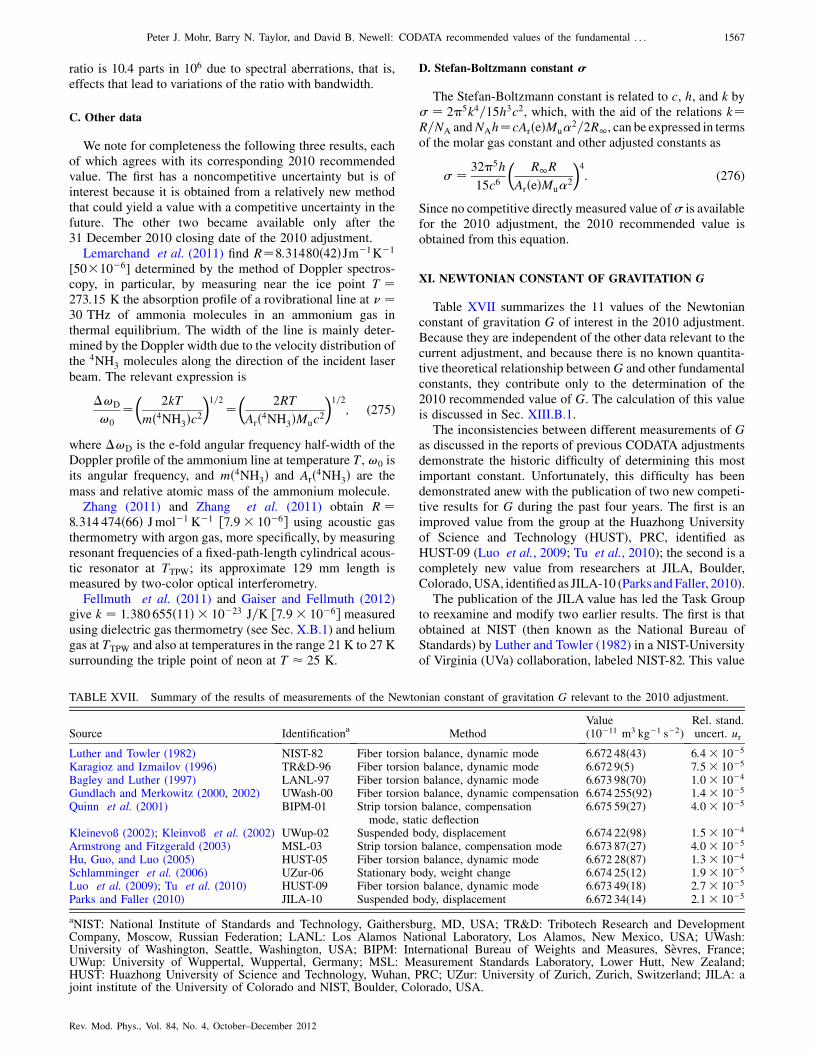
ratio is 10.4 parts in 106 due to spectral aberrations, that is,effects that lead to variations of the ratio with bandwidth.
C. Other data
We note for completeness the following three results, eachof which agrees with its corresponding 2010 recommendedvalue. The first has a noncompetitive uncertainty but is ofinterest because it is obtained from a relatively new methodthat could yield a value with a competitive uncertainty in thefuture. The other two became available only after the31 December 2010 closing date of the 2010 adjustment.
Lemarchand et al. (2011) find R¼8:31480ð42ÞJm�1K�1
[50�10�6] determined by the method of Doppler spectros-copy, in particular, by measuring near the ice point T ¼273:15 K the absorption profile of a rovibrational line at � ¼30 THz of ammonia molecules in an ammonium gas inthermal equilibrium. The width of the line is mainly deter-mined by the Doppler width due to the velocity distribution ofthe 4NH3 molecules along the direction of the incident laser
beam. The relevant expression is
�!D
!0
¼�
2kT
mð4NH3Þc2�1=2¼
�2RT
Arð4NH3ÞMuc2
�1=2
; (275)
where �!D is the e-fold angular frequency half-width of theDoppler profile of the ammonium line at temperature T,!0 isits angular frequency, and mð4NH3Þ and Arð4NH3Þ are the
mass and relative atomic mass of the ammonium molecule.Zhang (2011) and Zhang et al. (2011) obtain R ¼
8:314 474ð66Þ Jmol�1 K�1 ½7:9� 10�6� using acoustic gasthermometry with argon gas, more specifically, by measuringresonant frequencies of a fixed-path-length cylindrical acous-tic resonator at TTPW; its approximate 129 mm length ismeasured by two-color optical interferometry.
Fellmuth et al. (2011) and Gaiser and Fellmuth (2012)give k ¼ 1:380 655ð11Þ � 10�23 J=K ½7:9� 10�6� measuredusing dielectric gas thermometry (see Sec. X.B.1) and heliumgas at TTPW and also at temperatures in the range 21 K to 27 Ksurrounding the triple point of neon at T � 25 K.
D. Stefan-Boltzmann constant �
The Stefan-Boltzmann constant is related to c, h, and k by� ¼ 2�5k4=15h3c2, which, with the aid of the relations k¼R=NA andNAh¼cArðeÞMu�
2=2R1, can be expressed in termsof the molar gas constant and other adjusted constants as
� ¼ 32�5h
15c6
�R1R
ArðeÞMu�2
�4: (276)
Since no competitive directly measured value of� is availablefor the 2010 adjustment, the 2010 recommended value isobtained from this equation.
XI. NEWTONIAN CONSTANT OF GRAVITATION G
Table XVII summarizes the 11 values of the Newtonianconstant of gravitation G of interest in the 2010 adjustment.Because they are independent of the other data relevant to thecurrent adjustment, and because there is no known quantita-tive theoretical relationship betweenG and other fundamentalconstants, they contribute only to the determination of the2010 recommended value of G. The calculation of this valueis discussed in Sec. XIII.B.1.
The inconsistencies between different measurements of Gas discussed in the reports of previous CODATA adjustmentsdemonstrate the historic difficulty of determining this mostimportant constant. Unfortunately, this difficulty has beendemonstrated anew with the publication of two new competi-tive results for G during the past four years. The first is animproved value from the group at the Huazhong Universityof Science and Technology (HUST), PRC, identified asHUST-09 (Luo et al., 2009; Tu et al., 2010); the second is acompletely new value from researchers at JILA, Boulder,Colorado,USA, identified as JILA-10 (Parks and Faller, 2010).
The publication of the JILA value has led the Task Groupto reexamine and modify two earlier results. The first is thatobtained at NIST (then known as the National Bureau ofStandards) by Luther and Towler (1982) in a NIST-Universityof Virginia (UVa) collaboration, labeled NIST-82. This value
TABLE XVII. Summary of the results of measurements of the Newtonian constant of gravitation G relevant to the 2010 adjustment.
Source Identificationa MethodValue(10�11 m3 kg�1 s�2)
Rel. stand.uncert. ur
Luther and Towler (1982) NIST-82 Fiber torsion balance, dynamic mode 6.672 48(43) 6:4� 10�5
Karagioz and Izmailov (1996) TR&D-96 Fiber torsion balance, dynamic mode 6.672 9(5) 7:5� 10�5
Bagley and Luther (1997) LANL-97 Fiber torsion balance, dynamic mode 6.673 98(70) 1:0� 10�4
Gundlach and Merkowitz (2000, 2002) UWash-00 Fiber torsion balance, dynamic compensation 6.674 255(92) 1:4� 10�5
Quinn et al. (2001) BIPM-01 Strip torsion balance, compensationmode, static deflection
6.675 59(27) 4:0� 10�5
Kleinevoß (2002); Kleinvoß et al. (2002) UWup-02 Suspended body, displacement 6.674 22(98) 1:5� 10�4
Armstrong and Fitzgerald (2003) MSL-03 Strip torsion balance, compensation mode 6.673 87(27) 4:0� 10�5
Hu, Guo, and Luo (2005) HUST-05 Fiber torsion balance, dynamic mode 6.672 28(87) 1:3� 10�4
Schlamminger et al. (2006) UZur-06 Stationary body, weight change 6.674 25(12) 1:9� 10�5
Luo et al. (2009); Tu et al. (2010) HUST-09 Fiber torsion balance, dynamic mode 6.673 49(18) 2:7� 10�5
Parks and Faller (2010) JILA-10 Suspended body, displacement 6.672 34(14) 2:1� 10�5
aNIST: National Institute of Standards and Technology, Gaithersburg, MD, USA; TR&D: Tribotech Research and DevelopmentCompany, Moscow, Russian Federation; LANL: Los Alamos National Laboratory, Los Alamos, New Mexico, USA; UWash:University of Washington, Seattle, Washington, USA; BIPM: International Bureau of Weights and Measures, Sevres, France;UWup: University of Wuppertal, Wuppertal, Germany; MSL: Measurement Standards Laboratory, Lower Hutt, New Zealand;HUST: Huazhong University of Science and Technology, Wuhan, PRC; UZur: University of Zurich, Zurich, Switzerland; JILA: ajoint institute of the University of Colorado and NIST, Boulder, Colorado, USA.
Peter J. Mohr, Barry N. Taylor, and David B. Newell: CODATA recommended values of the fundamental . . . 1567
Rev. Mod. Phys., Vol. 84, No. 4, October–December 2012
was the basis for the CODATA 1986 recommended value(Cohen and Taylor, 1987) and was taken into account indetermining the CODATA 1998 value (Mohr and Taylor,2000), but played no role in either the 2002 or 2006 adjust-ments. The second is the Los Alamos National Laboratory(LANL), Los Alamos, USA, result of Bagley and Luther(1997), labeled LANL-97; it was first included in the 1998CODATA adjustment and in all subsequent adjustments. The11 available values of G, which are data items G1–G11 inTable XXIV, Sec. XIII, are the same as in 2006 with theexception of NIST-82, slightly modified LANL-97, and thetwo new values. Thus, in keeping with our approach in thisreport, there is no discussion of the other seven values sincethey have been covered in one or more of the previous reports.
For simplicity we write G as a numerical factor multi-plying G0, where
G0 ¼ 10�11 m3 kg�1 s�2: (277)
A. Updated values
1. National Institute of Standards and Technology and
University of Virginia
As discussed in CODATA-98, the experiment of Lutherand Towler (1982) used a fiber-based torsion balance oper-ated in the dynamic mode and the time-of-swing method,thereby requiring measurement of a small change in the longoscillation period of the balance. Ideally, the torsional springconstant of the fiber should be independent of frequency atvery low frequencies, for example, at 3 mHz.
Long after the publication of the NIST-UVa result, Kuroda(1995) [see also Matsumura et al. (1998) and Kuroda (1999)]pointed out that the anelasticity of such fibers is sufficientlylarge to cause the value of G determined in this way to bebiased. IfQ is the quality factor of the main torsional mode ofthe fiber and it is assumed that the damping of the torsionbalance is solely due to the losses in the fiber, then theunbiased value of G is related to the experimentally observedvalue GðobsÞ by (Kuroda, 1995)
G ¼ GðobsÞ1þ �Q
: (278)
Although the exact value of the Q of the fiber used in theNIST-UVa experiment is unknown, Luther (2010) providedan estimate, based on data obtained during the course of theexperiment, of no less than 10 000 and no greater than 30 000.Assuming a rectangular probability density function for Qwith these lower and upper limits then leads to Q ¼ 2� 104
with a relative standard uncertainty of 4:6�10�6. Using thesevalues, the result GðobsÞ¼6:67259ð43ÞG0 ½64� 10�6�(Luther and Towler, 1982; Luther, 1986), and Eq. (278) weobtain
G ¼ 6:672 48ð43ÞG0 ½6:4� 10�5�: (279)
In this case the correction 1=ð1þ �QÞ reduced GðobsÞ by thefractional amount 15:9ð4:6Þ � 10�6, but increased its 64�10�6 relative standard uncertainty by a negligible amount.
The Task Group decided to include the value given inEq. (279) as an input datum in the 2010 adjustment eventhough it was not included in the 2002 and 2006 adjustments,
because information provided by Luther (2010) allows theoriginal result to be corrected for the Kuroda effect. Further,although there were plans to continue the NIST-UVa experi-ment (Luther and Towler, 1982), recent conversations withLuther (2010) made clear that the measurements on which theresult is based were thorough and complete.
2. Los Alamos National Laboratory
The experiment of Bagley and Luther (1997), also de-scribed in detail in CODATA-98, is similar to the NIST-UVaexperiment of Luther and Towler (1982), and in fact usedsome of the same components including the tungsten sourcemasses. Its purpose was not only to determine G, but also totest the Kuroda hypothesis by using two different fibers, onewith Q ¼ 950 and the other with Q ¼ 490. Because the valueof G resulting from this experiment is correlated with theNIST-UVa value and both values are now being included inthe adjustment, we evaluated the correlation coefficient of thetwo results. This was done with information from Bagley(2010) and Luther (2010) and Bagley (1996). We also recal-culated the result of the experiment of Bagley and Luther(1997) by taking into account the uncertainties of the two Qvalues (2%) and the correlation coefficient of the two values ofG obtained from the two fibers (0.147) when computing theirweighted mean. The final value is
G ¼ 6:673 98ð70ÞG0 ½1:0� 10�4�; (280)
which in fact is essentially the same as the value used in the2002 and 2006 adjustments. The correlation coefficient of theNIST-UVa and LANL values of G is 0.351.
B. New values
1. Huazhong University of Science and Technology
The improved HUST-09 result for G was first reported byLuo et al. (2009) and subsequently described in detail by Tuet al. (2010); it represents a reduction in uncertainty, com-pared to the previous Huazhong University result HUST-05,of about a factor of 5. As pointed out by Tu et al. (2010), anumber of changes in the earlier experiment contributed tothis uncertainty reduction, including (i) replacement of thetwo stainless steel cylindrical source masses by sphericalsource masses with a more homogeneous density; (ii) useof a rectangular quartz block as the principal portion of thetorsion balance’s pendulum, thereby improving the stabilityof the period of the balance and reducing the uncertainty ofthe pendulum’s moment of inertia; (iii) a single vacuumchamber for the source masses and pendulum leading to areduction of the uncertainty of their relative positions; (iv) aremotely operated stepper motor to change the positions ofthe source masses, thereby reducing environmental changes;and (v) measurement of the anelasticity of the torsion fiberwith the aid of a high-Q quartz fiber.
The final result is the average of two values of G that differby 9 parts in 106 obtained from two partially correlateddeterminations using the same apparatus. The dominant com-ponents of uncertainty, in parts in 106, are 19 from themeasurement of the fiber’s anelasticity, 14 (statistical) fromthe measurement of the change in the square of the angularfrequency of the pendulum when the source masses are in
1568 Peter J. Mohr, Barry N. Taylor, and David B. Newell: CODATA recommended values of the fundamental . . .
Rev. Mod. Phys., Vol. 84, No. 4, October–December 2012
their near and far positions, and 10 from themeasured distancebetween the geometric centers of the source masses. Althoughthe uncertainty of HUST-05 is 5 times larger than that ofHUST-09, Luo (2010) and co-workers do not believe thatHUST-09 supersedes HUST-05. Thus, both are consideredfor inclusion in the 2010 adjustment. Based on informationprovided to the Task Group by the researchers (Luo, 2010),their correlation coefficient is estimated to be 0.234 and is usedin the calculations of Sec. XIII. The extra digits for the valueand uncertainty of HUST-05 were also provided by Luo(2011).
2. JILA
As can be seen from Table XVII, the 21� 10�6 relativestandard uncertainty of the value of G identified as JILA-10and obtained at JILA by Parks and Faller (2010) has the thirdsmallest estimated uncertainty of the values listed and is thesecond smallest of those values. It differs from the value withthe smallest uncertainty, identified as UWash-00, by 287(25)parts in 106, which is 11 times the standard uncertainty of theirdifference udiff , or 11�. This disagreement is an example of the‘‘historic difficulty’’ referred to at the very beginning of thissection. The data on which the JILA researchers based theirresult were taken in 2004, but being well aware of this incon-sistency they hesitated to publish it until they checked andrechecked their work (Parks and Faller, 2010). With this done,they decided it was time to report their value for G.
The apparatus used in the JILA experiment of Parks andFaller (2010) consisted of two 780 g copper test masses (or‘‘pendulum bobs’’) separated by 34 cm, each of which wassuspended from a supporting bar by four wires and togetherthey formed a Fabry-Perot cavity. When the four 120 kgcylindrical tungsten source masses, two pairs with each mem-ber of the pair on either side of the laser beam traversing thecavity, were periodicallymoved parallel to the laser beam fromtheir inner and outer positions (they remained stationary for80 s in each position), the separation between the bobs changedby about 90 nm. This change was observed as a 125 MHz beatfrequency between the laser locked to the pendulum cavity andthe laser locked to a reference cavity that was part of thesupporting bar. The geometry of the experiment reduces themost difficult aspect of determining the gravitational field ofthe source masses to six one dimensional measurements: thedistance between opposite source mass pairs in the inner andouter positions and the distances between adjacent sourcemasses in the inner position. The most important relativestandard uncertainty components contributing to the uncer-tainty ofG are, in parts in 106 (Parks and Faller, 2010), the sixcritical dimension measurements, 14; all other dimensionmeasurements and source mass density inhomogeneities,8 each; pendulum spring constants, 7; and total mass measure-ment and interferometer misalignment, 6 each.
XII. ELECTROWEAK QUANTITIES
As in previous adjustments, there are a few cases in the2010 adjustment where an inexact constant that is used inthe analysis of input data is not treated as an adjustedquantity, because the adjustment has a negligible effect onits value. Three such constants, used in the calculation of the
theoretical expression for the electron magnetic-momentanomaly ae, are the mass of the tau lepton m�, the Fermicoupling constant GF, and sine squared of the weak mixingangle sin2�W; they are obtained from the most recent reportof the Particle Data Group (Nakamura et al., 2010):
m�c2 ¼ 1776:82ð16Þ MeV ½9:0� 10�5�; (281)
GF=ðℏcÞ3 ¼ 1:166364ð5Þ�10�5 GeV�2 ½4:3�10�6�;(282)
sin2�W ¼ 0:2223ð21Þ ½9:5� 10�3�: (283)
The value for GF=ðℏcÞ3 is from Nakamura et al. (2010),p. 127. We use the definition sin2�W ¼ 1� ðmW=mZÞ2,where mW and mZ are, respectively, the masses of the Wand Z0 bosons, because it is employed in the calculation ofthe electroweak contributions to ae (Czarnecki, Krause, andMarciano, 1996). The Particle Data Group’s recommendedvalue for the mass ratio of these bosons is mW=mZ ¼0:8819ð12Þ, which leads to the value of sin2�W given above.
XIII. ANALYSIS OF DATA
We examine in this section the input data discussed in theprevious sections and, based upon that examination, select thedata to be used in the least-squares adjustment that deter-mines the 2010 CODATA recommended values of theconstants. Tables XVIII, XX, XXII, and XXIV give the inputdata, including the �’s, which are corrections added to theo-retical expressions to account for the uncertainties of thoseexpressions. The covariances of the data are given as corre-lation coefficients in Tables XIX, XXI, XXIII, and XXIV.There are 14 types of input data for which there are two ormore experiments, and the data of the same type generallyagree (values of G excepted).
A. Comparison of data through inferred values of
�, h, k, and ArðeÞ
Here the level of consistency of the data is shown bycomparing values of �, h, k, and ArðeÞ that can be inferredfrom different types of experiments. Note, however, that theinferred value is for comparison purposes only; the datumfrom which it is obtained, not the inferred value, is used as theinput datum in the least-squares calculations.
Table XXVand Figs. 1 and 2 compare values of � obtainedfrom the indicated input data. These values are calculatedusing the appropriate observational equation for each inputdatum as given in Table XXXIII and the 2010 recommendedvalues of the constants other than � that enter that equation.(Some inferred values have also been given where the rele-vant datum is discussed.) Inspection of the table and figuresshows that there is agreement among the vast majority of thevarious values of �, and hence the data from which they areobtained, to the extent that the difference between any twovalues of � is less than 2udiff , the standard uncertainty of thedifference.
The two exceptions are the values of � from the NIST-89result for �0
p�90ðloÞ and, to a lesser extent, the KR/VN-98
result for �0h�90ðloÞ; of the 91 differences, six involving �
Peter J. Mohr, Barry N. Taylor, and David B. Newell: CODATA recommended values of the fundamental . . . 1569
Rev. Mod. Phys., Vol. 84, No. 4, October–December 2012
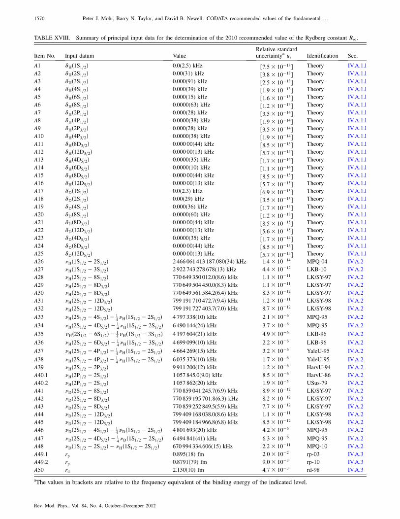
TABLE XVIII. Summary of principal input data for the determination of the 2010 recommended value of the Rydberg constant R1.
Item No. Input datum ValueRelative standarduncertaintya ur Identification Sec.
A1 �Hð1S1=2Þ 0.0(2.5) kHz ½7:5� 10�13� Theory IV.A.1.l
A2 �Hð2S1=2Þ 0.00(31) kHz ½3:8� 10�13� Theory IV.A.1.l
A3 �Hð3S1=2Þ 0.000(91) kHz ½2:5� 10�13� Theory IV.A.1.l
A4 �Hð4S1=2Þ 0.000(39) kHz ½1:9� 10�13� Theory IV.A.1.l
A5 �Hð6S1=2Þ 0.000(15) kHz ½1:6� 10�13� Theory IV.A.1.l
A6 �Hð8S1=2Þ 0.0000(63) kHz ½1:2� 10�13� Theory IV.A.1.l
A7 �Hð2P1=2Þ 0.000(28) kHz ½3:5� 10�14� Theory IV.A.1.l
A8 �Hð4P1=2Þ 0.0000(38) kHz ½1:9� 10�14� Theory IV.A.1.l
A9 �Hð2P3=2Þ 0.000(28) kHz ½3:5� 10�14� Theory IV.A.1.l
A10 �Hð4P3=2Þ 0.0000(38) kHz ½1:9� 10�14� Theory IV.A.1.l
A11 �Hð8D3=2Þ 0.000 00(44) kHz ½8:5� 10�15� Theory IV.A.1.l
A12 �Hð12D3=2Þ 0.000 00(13) kHz ½5:7� 10�15� Theory IV.A.1.l
A13 �Hð4D5=2Þ 0.0000(35) kHz ½1:7� 10�14� Theory IV.A.1.l
A14 �Hð6D5=2Þ 0.0000(10) kHz ½1:1� 10�14� Theory IV.A.1.l
A15 �Hð8D5=2Þ 0.000 00(44) kHz ½8:5� 10�15� Theory IV.A.1.l
A16 �Hð12D5=2Þ 0.000 00(13) kHz ½5:7� 10�15� Theory IV.A.1.l
A17 �Dð1S1=2Þ 0.0(2.3) kHz ½6:9� 10�13� Theory IV.A.1.l
A18 �Dð2S1=2Þ 0.00(29) kHz ½3:5� 10�13� Theory IV.A.1.l
A19 �Dð4S1=2Þ 0.000(36) kHz ½1:7� 10�13� Theory IV.A.1.l
A20 �Dð8S1=2Þ 0.0000(60) kHz ½1:2� 10�13� Theory IV.A.1.l
A21 �Dð8D3=2Þ 0.000 00(44) kHz ½8:5� 10�15� Theory IV.A.1.l
A22 �Dð12D3=2Þ 0.000 00(13) kHz ½5:6� 10�15� Theory IV.A.1.l
A23 �Dð4D5=2Þ 0.0000(35) kHz ½1:7� 10�14� Theory IV.A.1.l
A24 �Dð8D5=2Þ 0.000 00(44) kHz ½8:5� 10�15� Theory IV.A.1.l
A25 �Dð12D5=2Þ 0.000 00(13) kHz ½5:7� 10�15� Theory IV.A.1.l
A26 �Hð1S1=2 � 2S1=2Þ 2 466 061 413 187.080(34) kHz 1:4� 10�14 MPQ-04 IV.A.2
A27 �Hð1S1=2 � 3S1=2Þ 2 922 743 278 678(13) kHz 4:4� 10�12 LKB-10 IV.A.2
A28 �Hð2S1=2 � 8S1=2Þ 770 649 350 012.0(8.6) kHz 1:1� 10�11 LK/SY-97 IV.A.2
A29 �Hð2S1=2 � 8D3=2Þ 770 649 504 450.0(8.3) kHz 1:1� 10�11 LK/SY-97 IV.A.2
A30 �Hð2S1=2 � 8D5=2Þ 770 649 561 584.2(6.4) kHz 8:3� 10�12 LK/SY-97 IV.A.2
A31 �Hð2S1=2 � 12D3=2Þ 799 191 710 472.7(9.4) kHz 1:2� 10�11 LK/SY-98 IV.A.2
A32 �Hð2S1=2 � 12D5=2Þ 799 191 727 403.7(7.0) kHz 8:7� 10�12 LK/SY-98 IV.A.2
A33 �Hð2S1=2 � 4S1=2Þ � 14�Hð1S1=2 � 2S1=2Þ 4 797 338(10) kHz 2:1� 10�6 MPQ-95 IV.A.2
A34 �Hð2S1=2 � 4D5=2Þ � 14�Hð1S1=2 � 2S1=2Þ 6 490 144(24) kHz 3:7� 10�6 MPQ-95 IV.A.2
A35 �Hð2S1=2 � 6S1=2Þ � 14�Hð1S1=2 � 3S1=2Þ 4 197 604(21) kHz 4:9� 10�6 LKB-96 IV.A.2
A36 �Hð2S1=2 � 6D5=2Þ � 14�Hð1S1=2 � 3S1=2Þ 4 699 099(10) kHz 2:2� 10�6 LKB-96 IV.A.2
A37 �Hð2S1=2 � 4P1=2Þ � 14�Hð1S1=2 � 2S1=2Þ 4 664 269(15) kHz 3:2� 10�6 YaleU-95 IV.A.2
A38 �Hð2S1=2 � 4P3=2Þ � 14�Hð1S1=2 � 2S1=2Þ 6 035 373(10) kHz 1:7� 10�6 YaleU-95 IV.A.2
A39 �Hð2S1=2 � 2P3=2Þ 9 911 200(12) kHz 1:2� 10�6 HarvU-94 IV.A.2
A40:1 �Hð2P1=2 � 2S1=2Þ 1 057 845.0(9.0) kHz 8:5� 10�6 HarvU-86 IV.A.2
A40:2 �Hð2P1=2 � 2S1=2Þ 1 057 862(20) kHz 1:9� 10�5 USus-79 IV.A.2
A41 �Dð2S1=2 � 8S1=2Þ 770 859 041 245.7(6.9) kHz 8:9� 10�12 LK/SY-97 IV.A.2
A42 �Dð2S1=2 � 8D3=2Þ 770 859 195 701.8(6.3) kHz 8:2� 10�12 LK/SY-97 IV.A.2
A43 �Dð2S1=2 � 8D5=2Þ 770 859 252 849.5(5.9) kHz 7:7� 10�12 LK/SY-97 IV.A.2
A44 �Dð2S1=2 � 12D3=2Þ 799 409 168 038.0(8.6) kHz 1:1� 10�11 LK/SY-98 IV.A.2
A45 �Dð2S1=2 � 12D5=2Þ 799 409 184 966.8(6.8) kHz 8:5� 10�12 LK/SY-98 IV.A.2
A46 �Dð2S1=2 � 4S1=2Þ � 14�Dð1S1=2 � 2S1=2Þ 4 801 693(20) kHz 4:2� 10�6 MPQ-95 IV.A.2
A47 �Dð2S1=2 � 4D5=2Þ � 14�Dð1S1=2 � 2S1=2Þ 6 494 841(41) kHz 6:3� 10�6 MPQ-95 IV.A.2
A48 �Dð1S1=2 � 2S1=2Þ � �Hð1S1=2 � 2S1=2Þ 670 994 334.606(15) kHz 2:2� 10�11 MPQ-10 IV.A.2
A49:1 rp 0.895(18) fm 2:0� 10�2 rp-03 IV.A.3
A49:2 rp 0.8791(79) fm 9:0� 10�3 rp-10 IV.A.3
A50 rd 2.130(10) fm 4:7� 10�3 rd-98 IV.A.3
aThe values in brackets are relative to the frequency equivalent of the binding energy of the indicated level.
1570 Peter J. Mohr, Barry N. Taylor, and David B. Newell: CODATA recommended values of the fundamental . . .
Rev. Mod. Phys., Vol. 84, No. 4, October–December 2012
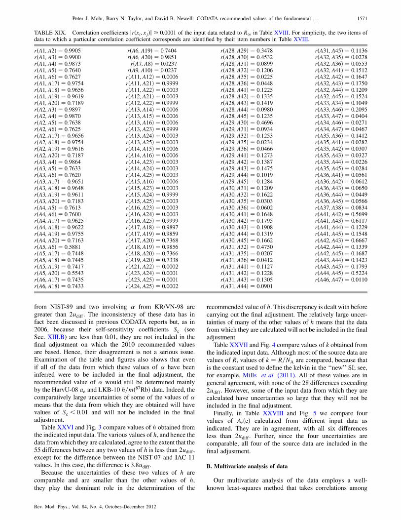
from NIST-89 and two involving � from KR/VN-98 aregreater than 2udiff . The inconsistency of these data has infact been discussed in previous CODATA reports but, as in2006, because their self-sensitivity coefficients Sc (seeSec. XIII.B) are less than 0.01, they are not included in thefinal adjustment on which the 2010 recommended valuesare based. Hence, their disagreement is not a serious issue.Examination of the table and figures also shows that evenif all of the data from which these values of � have beeninferred were to be included in the final adjustment, therecommended value of � would still be determined mainlyby the HarvU-08 ae and LKB-10 h=mð87RbÞ data. Indeed, thecomparatively large uncertainties of some of the values of �means that the data from which they are obtained will havevalues of Sc < 0:01 and will not be included in the finaladjustment.
Table XXVI and Fig. 3 compare values of h obtained fromthe indicated input data. The various values of h, and hence thedata fromwhich they are calculated, agree to the extent that the55 differences between any two values of h is less than 2udiff ,except for the difference between the NIST-07 and IAC-11values. In this case, the difference is 3:8udiff .
Because the uncertainties of these two values of h are
comparable and are smaller than the other values of h,they play the dominant role in the determination of the
recommended value of h. This discrepancy is dealt with beforecarrying out the final adjustment. The relatively large uncer-tainties of many of the other values of h means that the datafrom which they are calculated will not be included in the finaladjustment.
Table XXVII and Fig. 4 compare values of k obtained fromthe indicated input data. Although most of the source data arevalues of R, values of k ¼ R=NA are compared, because thatis the constant used to define the kelvin in the ‘‘new’’ SI; see,for example, Mills et al. (2011). All of these values are ingeneral agreement, with none of the 28 differences exceeding2udiff . However, some of the input data from which they arecalculated have uncertainties so large that they will not beincluded in the final adjustment.
Finally, in Table XXVIII and Fig. 5 we compare fourvalues of ArðeÞ calculated from different input data asindicated. They are in agreement, with all six differencesless than 2udiff . Further, since the four uncertainties arecomparable, all four of the source data are included in thefinal adjustment.
B. Multivariate analysis of data
Our multivariate analysis of the data employs a well-known least-squares method that takes correlations among
TABLE XIX. Correlation coefficients jrðxi; xjÞj � 0:0001 of the input data related to R1 in Table XVIII. For simplicity, the two items ofdata to which a particular correlation coefficient corresponds are identified by their item numbers in Table XVIII.
rðA1; A2Þ ¼ 0:9905 rðA6; A19Þ ¼ 0:7404 rðA28; A29Þ ¼ 0:3478 rðA31; A45Þ ¼ 0:1136rðA1; A3Þ ¼ 0:9900 rðA6; A20Þ ¼ 0:9851 rðA28; A30Þ ¼ 0:4532 rðA32; A35Þ ¼ 0:0278rðA1; A4Þ ¼ 0:9873 rðA7; A8Þ ¼ 0:0237 rðA28; A31Þ ¼ 0:0899 rðA32; A36Þ ¼ 0:0553rðA1; A5Þ ¼ 0:7640 rðA9; A10Þ ¼ 0:0237 rðA28; A32Þ ¼ 0:1206 rðA32; A41Þ ¼ 0:1512rðA1; A6Þ ¼ 0:7627 rðA11; A12Þ ¼ 0:0006 rðA28; A35Þ ¼ 0:0225 rðA32; A42Þ ¼ 0:1647rðA1; A17Þ ¼ 0:9754 rðA11; A21Þ ¼ 0:9999 rðA28; A36Þ ¼ 0:0448 rðA32; A43Þ ¼ 0:1750rðA1; A18Þ ¼ 0:9656 rðA11; A22Þ ¼ 0:0003 rðA28; A41Þ ¼ 0:1225 rðA32; A44Þ ¼ 0:1209rðA1; A19Þ ¼ 0:9619 rðA12; A21Þ ¼ 0:0003 rðA28; A42Þ ¼ 0:1335 rðA32; A45Þ ¼ 0:1524rðA1; A20Þ ¼ 0:7189 rðA12; A22Þ ¼ 0:9999 rðA28; A43Þ ¼ 0:1419 rðA33; A34Þ ¼ 0:1049rðA2; A3Þ ¼ 0:9897 rðA13; A14Þ ¼ 0:0006 rðA28; A44Þ ¼ 0:0980 rðA33; A46Þ ¼ 0:2095rðA2; A4Þ ¼ 0:9870 rðA13; A15Þ ¼ 0:0006 rðA28; A45Þ ¼ 0:1235 rðA33; A47Þ ¼ 0:0404rðA2; A5Þ ¼ 0:7638 rðA13; A16Þ ¼ 0:0006 rðA29; A30Þ ¼ 0:4696 rðA34; A46Þ ¼ 0:0271rðA2; A6Þ ¼ 0:7625 rðA13; A23Þ ¼ 0:9999 rðA29; A31Þ ¼ 0:0934 rðA34; A47Þ ¼ 0:0467rðA2; A17Þ ¼ 0:9656 rðA13; A24Þ ¼ 0:0003 rðA29; A32Þ ¼ 0:1253 rðA35; A36Þ ¼ 0:1412rðA2; A18Þ ¼ 0:9754 rðA13; A25Þ ¼ 0:0003 rðA29; A35Þ ¼ 0:0234 rðA35; A41Þ ¼ 0:0282rðA2; A19Þ ¼ 0:9616 rðA14; A15Þ ¼ 0:0006 rðA29; A36Þ ¼ 0:0466 rðA35; A42Þ ¼ 0:0307rðA2; A20Þ ¼ 0:7187 rðA14; A16Þ ¼ 0:0006 rðA29; A41Þ ¼ 0:1273 rðA35; A43Þ ¼ 0:0327rðA3; A4Þ ¼ 0:9864 rðA14; A23Þ ¼ 0:0003 rðA29; A42Þ ¼ 0:1387 rðA35; A44Þ ¼ 0:0226rðA3; A5Þ ¼ 0:7633 rðA14; A24Þ ¼ 0:0003 rðA29; A43Þ ¼ 0:1475 rðA35; A45Þ ¼ 0:0284rðA3; A6Þ ¼ 0:7620 rðA14; A25Þ ¼ 0:0003 rðA29; A44Þ ¼ 0:1019 rðA36; A41Þ ¼ 0:0561rðA3; A17Þ ¼ 0:9651 rðA15; A16Þ ¼ 0:0006 rðA29; A45Þ ¼ 0:1284 rðA36; A42Þ ¼ 0:0612rðA3; A18Þ ¼ 0:9648 rðA15; A23Þ ¼ 0:0003 rðA30; A31Þ ¼ 0:1209 rðA36; A43Þ ¼ 0:0650rðA3; A19Þ ¼ 0:9611 rðA15; A24Þ ¼ 0:9999 rðA30; A32Þ ¼ 0:1622 rðA36; A44Þ ¼ 0:0449rðA3; A20Þ ¼ 0:7183 rðA15; A25Þ ¼ 0:0003 rðA30; A35Þ ¼ 0:0303 rðA36; A45Þ ¼ 0:0566rðA4; A5Þ ¼ 0:7613 rðA16; A23Þ ¼ 0:0003 rðA30; A36Þ ¼ 0:0602 rðA37; A38Þ ¼ 0:0834rðA4; A6Þ ¼ 0:7600 rðA16; A24Þ ¼ 0:0003 rðA30; A41Þ ¼ 0:1648 rðA41; A42Þ ¼ 0:5699rðA4; A17Þ ¼ 0:9625 rðA16; A25Þ ¼ 0:9999 rðA30; A42Þ ¼ 0:1795 rðA41; A43Þ ¼ 0:6117rðA4; A18Þ ¼ 0:9622 rðA17; A18Þ ¼ 0:9897 rðA30; A43Þ ¼ 0:1908 rðA41; A44Þ ¼ 0:1229rðA4; A19Þ ¼ 0:9755 rðA17; A19Þ ¼ 0:9859 rðA30; A44Þ ¼ 0:1319 rðA41; A45Þ ¼ 0:1548rðA4; A20Þ ¼ 0:7163 rðA17; A20Þ ¼ 0:7368 rðA30; A45Þ ¼ 0:1662 rðA42; A43Þ ¼ 0:6667rðA5; A6Þ ¼ 0:5881 rðA18; A19Þ ¼ 0:9856 rðA31; A32Þ ¼ 0:4750 rðA42; A44Þ ¼ 0:1339rðA5; A17Þ ¼ 0:7448 rðA18; A20Þ ¼ 0:7366 rðA31; A35Þ ¼ 0:0207 rðA42; A45Þ ¼ 0:1687rðA5; A18Þ ¼ 0:7445 rðA19; A20Þ ¼ 0:7338 rðA31; A36Þ ¼ 0:0412 rðA43; A44Þ ¼ 0:1423rðA5; A19Þ ¼ 0:7417 rðA21; A22Þ ¼ 0:0002 rðA31; A41Þ ¼ 0:1127 rðA43; A45Þ ¼ 0:1793rðA5; A20Þ ¼ 0:5543 rðA23; A24Þ ¼ 0:0001 rðA31; A42Þ ¼ 0:1228 rðA44; A45Þ ¼ 0:5224rðA6; A17Þ ¼ 0:7435 rðA23; A25Þ ¼ 0:0001 rðA31; A43Þ ¼ 0:1305 rðA46; A47Þ ¼ 0:0110rðA6; A18Þ ¼ 0:7433 rðA24; A25Þ ¼ 0:0002 rðA31; A44Þ ¼ 0:0901
Peter J. Mohr, Barry N. Taylor, and David B. Newell: CODATA recommended values of the fundamental . . . 1571
Rev. Mod. Phys., Vol. 84, No. 4, October–December 2012
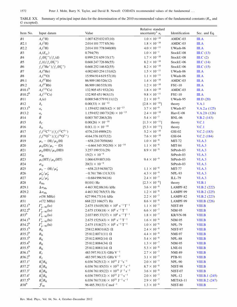
TABLE XX. Summary of principal input data for the determination of the 2010 recommended values of the fundamental constants (R1 andG excepted).
Item No. Input datum ValueRelative standarduncertaintya ur Identification Sec. and Eq.
B1 Arð1HÞ 1.007 825 032 07(10) 1:0� 10�10 AMDC-03 III.A
B2:1 Arð2HÞ 2.014 101 777 85(36) 1:8� 10�10 AMDC-03 III.A
B2:2 Arð2HÞ 2.014 101 778 040(80) 4:0� 10�11 UWash-06 III.A
B3 ArðEavÞ 0.794(79) 1:0� 10�1 StockU-08 III.C (13)
B4 fcðHþ�2 Þ=fcðdÞ 0.999 231 659 33(17) 1:7� 10�10 StockU-08 III.C (2)
B5 fcðtÞ=fcðHþ�2 Þ 0.668 247 726 86(55) 8:2� 10�10 StockU-06 III.C (14)
B6 fcð3HeþÞ=fcðHþ�2 Þ 0.668 252 146 82(55) 8:2� 10�10 StockU-06 III.C (15)
B7 Arð4HeÞ 4.002 603 254 131(62) 1:5� 10�11 UWash-06 III.A
B8 Arð16OÞ 15.994 914 619 57(18) 1:1� 10�11 UWash-06 III.A
B9:1 Arð87RbÞ 86.909 180 526(12) 1:4� 10�10 AMDC-03 III.A
B9:2 Arð87RbÞ 86.909 180 535(10) 1:2� 10�10 FSU-10 III.A
B10:1b Arð133CsÞ 132.905 451 932(24) 1:8� 10�10 AMDC-03 III.A
B10:2b Arð133CsÞ 132.905 451 963(13) 9:8� 10�11 FSU-10 III.A
B11 ArðeÞ 0.000 548 579 9111(12) 2:1� 10�9 UWash-95 III.D (20)
B12 �e 0:00ð33Þ � 10�12 [2:8� 10�10] theory V.A.1
B13:1b ae 1:159 652 1883ð42Þ � 10�13 3:7� 10�9 UWash-87 V.A.2.a (125)
B13:2 ae 1:159 652 180 73ð28Þ � 10�13 2:4� 10�10 HarvU-08 V.A.2.b (126)
B14 �R 0.003 707 2063(20) 5:4� 10�7 BNL-06 V.B.2 (143)
B15 �C 0:00ð26Þ � 10�10 [1:3� 10�11] theory V.C.1
B16 �O 0:0ð1:1Þ � 10�10 [5:3� 10�11] theory V.C.1
B17 fsð12C5þÞ=fcð12C5þÞ 4376.210 4989(23) 5:2� 10�10 GSI-02 V.C.2 (183)
B18 fsð16O7þÞ=fcð16O7þÞ 4164.376 1837(32) 7:6� 10�10 GSI-04 V.C.2 (184)
B19 �e � ðHÞ=�pðHÞ �658:210 7058ð66Þ 1:0� 10�8 MIT-72 VI.A.3
B20 �dðDÞ=�e � ðDÞ �4:664 345 392ð50Þ � 10�14 1:1� 10�8 MIT-84 VI.A.3
B21 �pðHDÞ=�dðHDÞ 3.257 199 531(29) 8:9� 10�9 StPtrsb-03 VI.A.3
B22 �dp 15ð2Þ � 10�9 StPtrsb-03 VI.A.3
B23 �tðHTÞ=�pðHTÞ 1.066 639 887(10) 9:4� 10�9 StPtrsb-03 VI.A.3
B24 �tp 20ð3Þ � 10�9 StPtrsb-03 VI.A.3
B25 �e � ðHÞ=�0p �658:215 9430ð72Þ 1:1� 10�8 MIT-77 VI.A.3
B26 �0h=�
0p �0:761 786 1313ð33Þ 4:3� 10�9 NPL-93 VI.A.3
B27 �0n=�
0p �0:684 996 94ð16Þ 2:4� 10�7 ILL-79 VI.A.3
B28 �Mu 0ð101Þ Hz [2:3� 10�8] theory VI.B.1
B29:1 ��Mu 4 463 302.88(16) kHz 3:6� 10�8 LAMPF-82 VI.B.2 (222)
B29:2 ��Mu 4 463 302 765(53) Hz 1:2� 10�8 LAMPF-99 VI.B.2 (225)
B30 �ð58 MHzÞ 627 994.77(14) kHz 2:2� 10�7 LAMPF-82 VI.B.2 (223)
B31 �ð72 MHzÞ 668 223 166(57) Hz 8:6� 10�8 LAMPF-99 VIII.B (226)
B32:1b �0p�90ðloÞ 2:675 154 05ð30Þ � 108 s�1 T�1 1:1� 10�7 NIST-89 VIII.B
B32:2b �0p�90ðloÞ 2:675 1530ð18Þ � 108 s�1 T�1 6:6� 10�7 NIM-95 VIII.B
B33b �0h�90ðloÞ 2:037 895 37ð37Þ � 108 s�1 T�1 1:8� 10�7 KR/VN-98 VIII.B
B34:1b �0p�90ðhiÞ 2:675 1525ð43Þ � 108 s�1 T�1 1:6� 10�6 NIM-95 VIII.B
B34:2b �0p�90ðhiÞ 2:675 1518ð27Þ � 108 s�1 T�1 1:0� 10�6 NPL-79 VIII.B
B35:1b RK 25812:80831ð62Þ � 2:4� 10�8 NIST-97 VIII.B
B35:2b RK 25 812:8071ð11Þ � 4:4� 10�8 NMI-97 VIII.B
B35:3b RK 25 812:8092ð14Þ � 5:4� 10�8 NPL-88 VIII.B
B35:4b RK 25 812:8084ð34Þ � 1:3� 10�7 NIM-95 VIII.B
B35:5b RK 25 812:8081ð14Þ � 5:3� 10�8 LNE-01 VIII.B
B36:1b KJ 483 597:91ð13Þ GHzV�1 2:7� 10�7 NMI-89 VIII.B
B36:2b KJ 483 597:96ð15Þ GHzV�1 3:1� 10�7 PTB-91 VIII.B
B37:1c K2JRK 6:036 7625ð12Þ � 1033 J�1s�1 2:0� 10�7 NPL-90 VIII.B
B37:2c K2JRK 6:036 761 85ð53Þ � 1033 J�1 s�1 8:7� 10�8 NIST-98 VIII.B
B37:3c K2JRK 6:036 761 85ð22Þ � 1033 J�1 s�1 3:6� 10�8 NIST-07 VIII.B
B37:4c K2JRK 6:036 7597ð12Þ � 1033 J�1 s�1 2:0� 10�7 NPL-12 VIII.B.1 (245)
B37:5b K2JRK 6:036 7617ð18Þ � 1033 J�1 s�1 2:9� 10�7 METAS-11 VIII.B.2 (247)
B38b F 90 96 485:39ð13Þ Cmol�1 1:3� 10�6 NIST-80 VIII.B
1572 Peter J. Mohr, Barry N. Taylor, and David B. Newell: CODATA recommended values of the fundamental . . .
Rev. Mod. Phys., Vol. 84, No. 4, October–December 2012
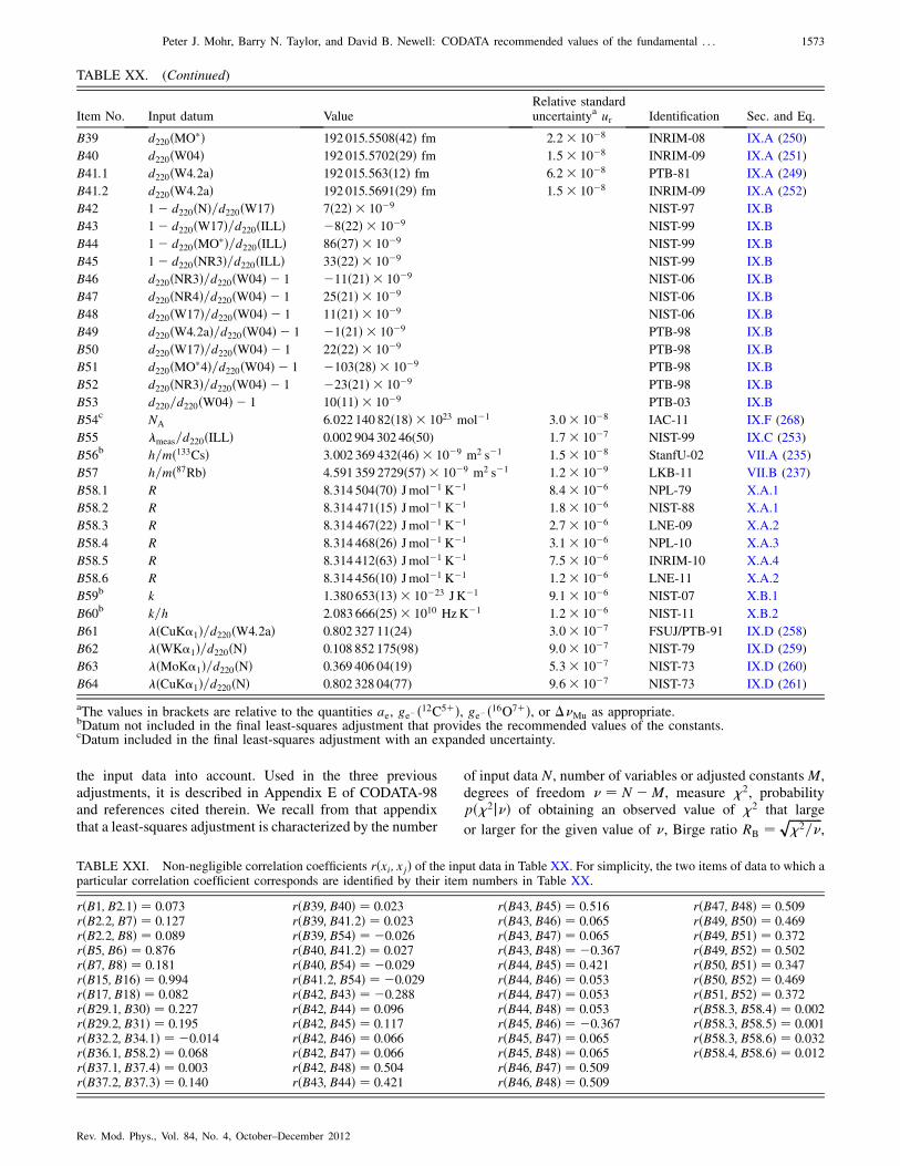
the input data into account. Used in the three previousadjustments, it is described in Appendix E of CODATA-98and references cited therein. We recall from that appendixthat a least-squares adjustment is characterized by the number
of input data N, number of variables or adjusted constantsM,degrees of freedom � ¼ N �M, measure �2, probabilitypð�2j�Þ of obtaining an observed value of �2 that large
or larger for the given value of �, Birge ratio RB ¼ ffiffiffiffiffiffiffiffiffiffiffi�2=�
p,
TABLE XXI. Non-negligible correlation coefficients rðxi; xjÞ of the input data in Table XX. For simplicity, the two items of data to which aparticular correlation coefficient corresponds are identified by their item numbers in Table XX.
rðB1; B2:1Þ ¼ 0:073 rðB39; B40Þ ¼ 0:023 rðB43; B45Þ ¼ 0:516 rðB47; B48Þ ¼ 0:509rðB2:2; B7Þ ¼ 0:127 rðB39; B41:2Þ ¼ 0:023 rðB43; B46Þ ¼ 0:065 rðB49; B50Þ ¼ 0:469rðB2:2; B8Þ ¼ 0:089 rðB39; B54Þ ¼ �0:026 rðB43; B47Þ ¼ 0:065 rðB49; B51Þ ¼ 0:372rðB5; B6Þ ¼ 0:876 rðB40; B41:2Þ ¼ 0:027 rðB43; B48Þ ¼ �0:367 rðB49; B52Þ ¼ 0:502rðB7; B8Þ ¼ 0:181 rðB40; B54Þ ¼ �0:029 rðB44; B45Þ ¼ 0:421 rðB50; B51Þ ¼ 0:347rðB15; B16Þ ¼ 0:994 rðB41:2; B54Þ ¼ �0:029 rðB44; B46Þ ¼ 0:053 rðB50; B52Þ ¼ 0:469rðB17; B18Þ ¼ 0:082 rðB42; B43Þ ¼ �0:288 rðB44; B47Þ ¼ 0:053 rðB51; B52Þ ¼ 0:372rðB29:1; B30Þ ¼ 0:227 rðB42; B44Þ ¼ 0:096 rðB44; B48Þ ¼ 0:053 rðB58:3; B58:4Þ ¼ 0:002rðB29:2; B31Þ ¼ 0:195 rðB42; B45Þ ¼ 0:117 rðB45; B46Þ ¼ �0:367 rðB58:3; B58:5Þ ¼ 0:001rðB32:2; B34:1Þ ¼ �0:014 rðB42; B46Þ ¼ 0:066 rðB45; B47Þ ¼ 0:065 rðB58:3; B58:6Þ ¼ 0:032rðB36:1; B58:2Þ ¼ 0:068 rðB42; B47Þ ¼ 0:066 rðB45; B48Þ ¼ 0:065 rðB58:4; B58:6Þ ¼ 0:012rðB37:1; B37:4Þ ¼ 0:003 rðB42; B48Þ ¼ 0:504 rðB46; B47Þ ¼ 0:509rðB37:2; B37:3Þ ¼ 0:140 rðB43; B44Þ ¼ 0:421 rðB46; B48Þ ¼ 0:509
Item No. Input datum ValueRelative standarduncertaintya ur Identification Sec. and Eq.
B39 d220ðMO�Þ 192 015:5508ð42Þ fm 2:2� 10�8 INRIM-08 IX.A (250)
B40 d220ðW04Þ 192 015:5702ð29Þ fm 1:5� 10�8 INRIM-09 IX.A (251)
B41:1 d220ðW4:2aÞ 192 015:563ð12Þ fm 6:2� 10�8 PTB-81 IX.A (249)
B41:2 d220ðW4:2aÞ 192 015:5691ð29Þ fm 1:5� 10�8 INRIM-09 IX.A (252)
B42 1� d220ðNÞ=d220ðW17Þ 7ð22Þ � 10�9 NIST-97 IX.B
B43 1� d220ðW17Þ=d220ðILLÞ �8ð22Þ � 10�9 NIST-99 IX.B
B44 1� d220ðMO�Þ=d220ðILLÞ 86ð27Þ � 10�9 NIST-99 IX.B
B45 1� d220ðNR3Þ=d220ðILLÞ 33ð22Þ � 10�9 NIST-99 IX.B
B46 d220ðNR3Þ=d220ðW04Þ � 1 �11ð21Þ � 10�9 NIST-06 IX.B
B47 d220ðNR4Þ=d220ðW04Þ � 1 25ð21Þ � 10�9 NIST-06 IX.B
B48 d220ðW17Þ=d220ðW04Þ � 1 11ð21Þ � 10�9 NIST-06 IX.B
B49 d220ðW4:2aÞ=d220ðW04Þ � 1 �1ð21Þ � 10�9 PTB-98 IX.B
B50 d220ðW17Þ=d220ðW04Þ � 1 22ð22Þ � 10�9 PTB-98 IX.B
B51 d220ðMO�4Þ=d220ðW04Þ � 1 �103ð28Þ � 10�9 PTB-98 IX.B
B52 d220ðNR3Þ=d220ðW04Þ � 1 �23ð21Þ � 10�9 PTB-98 IX.B
B53 d220=d220ðW04Þ � 1 10ð11Þ � 10�9 PTB-03 IX.B
B54c NA 6:022 140 82ð18Þ � 1023 mol�1 3:0� 10�8 IAC-11 IX.F (268)
B55 meas=d220ðILLÞ 0.002 904 302 46(50) 1:7� 10�7 NIST-99 IX.C (253)
B56b h=mð133CsÞ 3:002 369 432ð46Þ � 10�9 m2 s�1 1:5� 10�8 StanfU-02 VII.A (235)
B57 h=mð87RbÞ 4:591 359 2729ð57Þ � 10�9 m2 s�1 1:2� 10�9 LKB-11 VII.B (237)
B58:1 R 8:314 504ð70Þ Jmol�1 K�1 8:4� 10�6 NPL-79 X.A.1
B58:2 R 8:314 471ð15Þ Jmol�1 K�1 1:8� 10�6 NIST-88 X.A.1
B58:3 R 8:314 467ð22Þ Jmol�1 K�1 2:7� 10�6 LNE-09 X.A.2
B58:4 R 8:314 468ð26Þ Jmol�1 K�1 3:1� 10�6 NPL-10 X.A.3
B58:5 R 8:314 412ð63Þ Jmol�1 K�1 7:5� 10�6 INRIM-10 X.A.4
B58:6 R 8:314 456ð10Þ Jmol�1 K�1 1:2� 10�6 LNE-11 X.A.2
B59b k 1:380 653ð13Þ � 10�23 J K�1 9:1� 10�6 NIST-07 X.B.1
B60b k=h 2:083 666ð25Þ � 1010 HzK�1 1:2� 10�6 NIST-11 X.B.2
B61 ðCuK�1Þ=d220ðW4:2aÞ 0.802 327 11(24) 3:0� 10�7 FSUJ/PTB-91 IX.D (258)
B62 ðWK�1Þ=d220ðNÞ 0.108 852 175(98) 9:0� 10�7 NIST-79 IX.D (259)
B63 ðMoK�1Þ=d220ðNÞ 0.369 406 04(19) 5:3� 10�7 NIST-73 IX.D (260)
B64 ðCuK�1Þ=d220ðNÞ 0.802 328 04(77) 9:6� 10�7 NIST-73 IX.D (261)
aThe values in brackets are relative to the quantities ae, ge�ð12C5þÞ, ge�ð16O7þÞ, or ��Mu as appropriate.bDatum not included in the final least-squares adjustment that provides the recommended values of the constants.cDatum included in the final least-squares adjustment with an expanded uncertainty.
TABLE XX. (Continued)
Peter J. Mohr, Barry N. Taylor, and David B. Newell: CODATA recommended values of the fundamental . . . 1573
Rev. Mod. Phys., Vol. 84, No. 4, October–December 2012
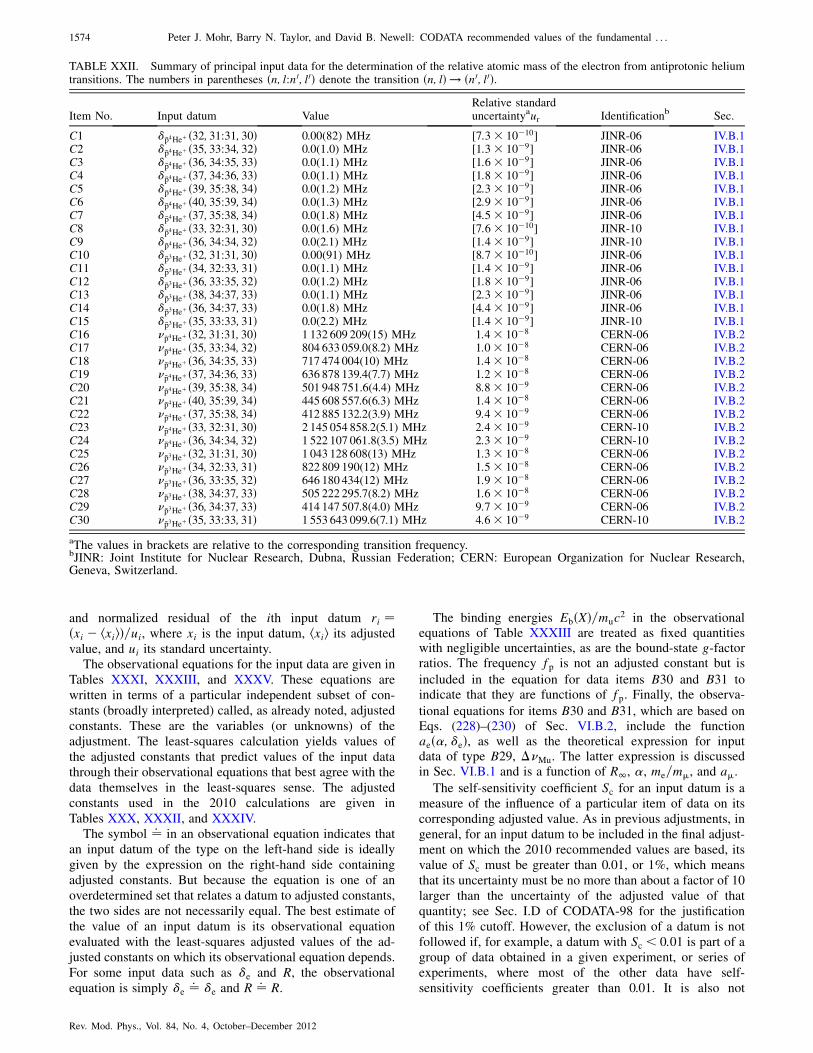
and normalized residual of the ith input datum ri ¼ðxi � hxiiÞ=ui, where xi is the input datum, hxii its adjustedvalue, and ui its standard uncertainty.
The observational equations for the input data are given inTables XXXI, XXXIII, and XXXV. These equations arewritten in terms of a particular independent subset of con-stants (broadly interpreted) called, as already noted, adjustedconstants. These are the variables (or unknowns) of theadjustment. The least-squares calculation yields values ofthe adjusted constants that predict values of the input datathrough their observational equations that best agree with thedata themselves in the least-squares sense. The adjustedconstants used in the 2010 calculations are given inTables XXX, XXXII, and XXXIV.
The symbol ¼: in an observational equation indicates thatan input datum of the type on the left-hand side is ideallygiven by the expression on the right-hand side containingadjusted constants. But because the equation is one of anoverdetermined set that relates a datum to adjusted constants,the two sides are not necessarily equal. The best estimate ofthe value of an input datum is its observational equationevaluated with the least-squares adjusted values of the ad-justed constants on which its observational equation depends.For some input data such as �e and R, the observationalequation is simply �e ¼: �e and R ¼: R.
The binding energies EbðXÞ=muc2 in the observational
equations of Table XXXIII are treated as fixed quantitieswith negligible uncertainties, as are the bound-state g-factorratios. The frequency fp is not an adjusted constant but is
included in the equation for data items B30 and B31 toindicate that they are functions of fp. Finally, the observa-
tional equations for items B30 and B31, which are based onEqs. (228)–(230) of Sec. VI.B.2, include the functionaeð�; �eÞ, as well as the theoretical expression for inputdata of type B29, ��Mu. The latter expression is discussedin Sec. VI.B.1 and is a function of R1, �, me=m�, and a�.
The self-sensitivity coefficient Sc for an input datum is ameasure of the influence of a particular item of data on itscorresponding adjusted value. As in previous adjustments, ingeneral, for an input datum to be included in the final adjust-ment on which the 2010 recommended values are based, itsvalue of Sc must be greater than 0.01, or 1%, which meansthat its uncertainty must be no more than about a factor of 10larger than the uncertainty of the adjusted value of thatquantity; see Sec. I.D of CODATA-98 for the justificationof this 1% cutoff. However, the exclusion of a datum is notfollowed if, for example, a datum with Sc < 0:01 is part of agroup of data obtained in a given experiment, or series ofexperiments, where most of the other data have self-sensitivity coefficients greater than 0.01. It is also not
TABLE XXII. Summary of principal input data for the determination of the relative atomic mass of the electron from antiprotonic heliumtransitions. The numbers in parentheses ðn; l:n0; l0Þ denote the transition ðn; lÞ ! ðn0; l0Þ.
Item No. Input datum ValueRelative standarduncertaintyaur Identificationb Sec.
C1 ��p4Heþ ð32; 31:31; 30Þ 0.00(82) MHz [7:3� 10�10] JINR-06 IV.B.1C2 ��p4Heþ ð35; 33:34; 32Þ 0.0(1.0) MHz [1:3� 10�9] JINR-06 IV.B.1C3 ��p4Heþ ð36; 34:35; 33Þ 0.0(1.1) MHz [1:6� 10�9] JINR-06 IV.B.1C4 ��p4Heþ ð37; 34:36; 33Þ 0.0(1.1) MHz [1:8� 10�9] JINR-06 IV.B.1C5 ��p4Heþ ð39; 35:38; 34Þ 0.0(1.2) MHz [2:3� 10�9] JINR-06 IV.B.1C6 ��p4Heþ ð40; 35:39; 34Þ 0.0(1.3) MHz [2:9� 10�9] JINR-06 IV.B.1C7 ��p4Heþ ð37; 35:38; 34Þ 0.0(1.8) MHz [4:5� 10�9] JINR-06 IV.B.1C8 ��p4Heþ ð33; 32:31; 30Þ 0.0(1.6) MHz [7:6� 10�10] JINR-10 IV.B.1C9 ��p4Heþ ð36; 34:34; 32Þ 0.0(2.1) MHz [1:4� 10�9] JINR-10 IV.B.1C10 ��p3Heþ ð32; 31:31; 30Þ 0.00(91) MHz [8:7� 10�10] JINR-06 IV.B.1C11 ��p3Heþ ð34; 32:33; 31Þ 0.0(1.1) MHz [1:4� 10�9] JINR-06 IV.B.1C12 ��p3Heþ ð36; 33:35; 32Þ 0.0(1.2) MHz [1:8� 10�9] JINR-06 IV.B.1C13 ��p3Heþ ð38; 34:37; 33Þ 0.0(1.1) MHz [2:3� 10�9] JINR-06 IV.B.1C14 ��p3Heþ ð36; 34:37; 33Þ 0.0(1.8) MHz [4:4� 10�9] JINR-06 IV.B.1C15 ��p3Heþ ð35; 33:33; 31Þ 0.0(2.2) MHz [1:4� 10�9] JINR-10 IV.B.1C16 ��p4Heþ ð32; 31:31; 30Þ 1 132 609 209(15) MHz 1:4� 10�8 CERN-06 IV.B.2C17 ��p4Heþ ð35; 33:34; 32Þ 804 633 059.0(8.2) MHz 1:0� 10�8 CERN-06 IV.B.2C18 ��p4Heþ ð36; 34:35; 33Þ 717 474 004(10) MHz 1:4� 10�8 CERN-06 IV.B.2C19 ��p4Heþ ð37; 34:36; 33Þ 636 878 139.4(7.7) MHz 1:2� 10�8 CERN-06 IV.B.2C20 ��p4Heþ ð39; 35:38; 34Þ 501 948 751.6(4.4) MHz 8:8� 10�9 CERN-06 IV.B.2C21 ��p4Heþ ð40; 35:39; 34Þ 445 608 557.6(6.3) MHz 1:4� 10�8 CERN-06 IV.B.2C22 ��p4Heþ ð37; 35:38; 34Þ 412 885 132.2(3.9) MHz 9:4� 10�9 CERN-06 IV.B.2C23 ��p4Heþ ð33; 32:31; 30Þ 2 145 054 858.2(5.1) MHz 2:4� 10�9 CERN-10 IV.B.2C24 ��p4Heþ ð36; 34:34; 32Þ 1 522 107 061.8(3.5) MHz 2:3� 10�9 CERN-10 IV.B.2C25 ��p3Heþ ð32; 31:31; 30Þ 1 043 128 608(13) MHz 1:3� 10�8 CERN-06 IV.B.2C26 ��p3Heþ ð34; 32:33; 31Þ 822 809 190(12) MHz 1:5� 10�8 CERN-06 IV.B.2C27 ��p3Heþ ð36; 33:35; 32Þ 646 180 434(12) MHz 1:9� 10�8 CERN-06 IV.B.2C28 ��p3Heþ ð38; 34:37; 33Þ 505 222 295.7(8.2) MHz 1:6� 10�8 CERN-06 IV.B.2C29 ��p3Heþ ð36; 34:37; 33Þ 414 147 507.8(4.0) MHz 9:7� 10�9 CERN-06 IV.B.2C30 ��p3Heþ ð35; 33:33; 31Þ 1 553 643 099.6(7.1) MHz 4:6� 10�9 CERN-10 IV.B.2
aThe values in brackets are relative to the corresponding transition frequency.bJINR: Joint Institute for Nuclear Research, Dubna, Russian Federation; CERN: European Organization for Nuclear Research,Geneva, Switzerland.
1574 Peter J. Mohr, Barry N. Taylor, and David B. Newell: CODATA recommended values of the fundamental . . .
Rev. Mod. Phys., Vol. 84, No. 4, October–December 2012
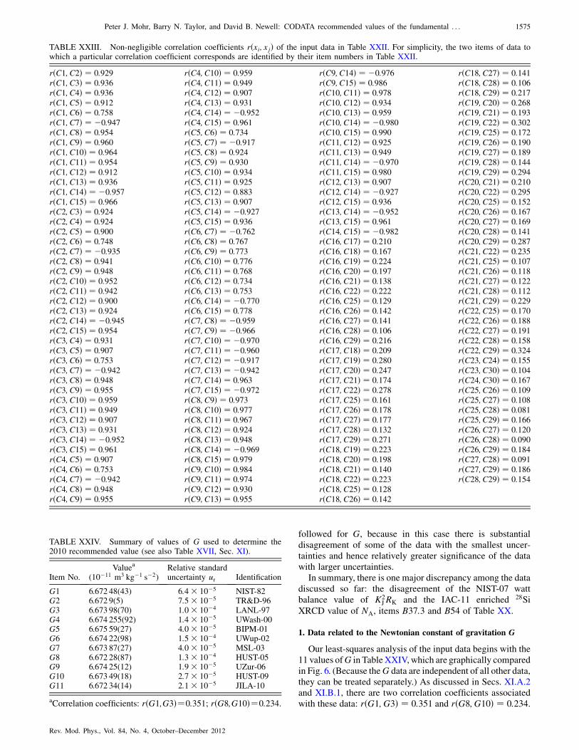
followed for G, because in this case there is substantialdisagreement of some of the data with the smallest uncer-tainties and hence relatively greater significance of the datawith larger uncertainties.
In summary, there is one major discrepancy among the datadiscussed so far: the disagreement of the NIST-07 wattbalance value of K2
JRK and the IAC-11 enriched 28SiXRCD value of NA, items B37:3 and B54 of Table XX.
1. Data related to the Newtonian constant of gravitation G
Our least-squares analysis of the input data begins with the11 values ofG in TableXXIV,which are graphically comparedin Fig. 6. (Because theG data are independent of all other data,they can be treated separately.) As discussed in Secs. XI.A.2and XI.B.1, there are two correlation coefficients associatedwith these data: rðG1; G3Þ ¼ 0:351 and rðG8; G10Þ ¼ 0:234.
TABLE XXIII. Non-negligible correlation coefficients rðxi; xjÞ of the input data in Table XXII. For simplicity, the two items of data towhich a particular correlation coefficient corresponds are identified by their item numbers in Table XXII.
rðC1; C2Þ ¼ 0:929 rðC4; C10Þ ¼ 0:959 rðC9; C14Þ ¼ �0:976 rðC18; C27Þ ¼ 0:141rðC1; C3Þ ¼ 0:936 rðC4; C11Þ ¼ 0:949 rðC9; C15Þ ¼ 0:986 rðC18; C28Þ ¼ 0:106rðC1; C4Þ ¼ 0:936 rðC4; C12Þ ¼ 0:907 rðC10; C11Þ ¼ 0:978 rðC18; C29Þ ¼ 0:217rðC1; C5Þ ¼ 0:912 rðC4; C13Þ ¼ 0:931 rðC10; C12Þ ¼ 0:934 rðC19; C20Þ ¼ 0:268rðC1; C6Þ ¼ 0:758 rðC4; C14Þ ¼ �0:952 rðC10; C13Þ ¼ 0:959 rðC19; C21Þ ¼ 0:193rðC1; C7Þ ¼ �0:947 rðC4; C15Þ ¼ 0:961 rðC10; C14Þ ¼ �0:980 rðC19; C22Þ ¼ 0:302rðC1; C8Þ ¼ 0:954 rðC5; C6Þ ¼ 0:734 rðC10; C15Þ ¼ 0:990 rðC19; C25Þ ¼ 0:172rðC1; C9Þ ¼ 0:960 rðC5; C7Þ ¼ �0:917 rðC11; C12Þ ¼ 0:925 rðC19; C26Þ ¼ 0:190rðC1; C10Þ ¼ 0:964 rðC5; C8Þ ¼ 0:924 rðC11; C13Þ ¼ 0:949 rðC19; C27Þ ¼ 0:189rðC1; C11Þ ¼ 0:954 rðC5; C9Þ ¼ 0:930 rðC11; C14Þ ¼ �0:970 rðC19; C28Þ ¼ 0:144rðC1; C12Þ ¼ 0:912 rðC5; C10Þ ¼ 0:934 rðC11; C15Þ ¼ 0:980 rðC19; C29Þ ¼ 0:294rðC1; C13Þ ¼ 0:936 rðC5; C11Þ ¼ 0:925 rðC12; C13Þ ¼ 0:907 rðC20; C21Þ ¼ 0:210rðC1; C14Þ ¼ �0:957 rðC5; C12Þ ¼ 0:883 rðC12; C14Þ ¼ �0:927 rðC20; C22Þ ¼ 0:295rðC1; C15Þ ¼ 0:966 rðC5; C13Þ ¼ 0:907 rðC12; C15Þ ¼ 0:936 rðC20; C25Þ ¼ 0:152rðC2; C3Þ ¼ 0:924 rðC5; C14Þ ¼ �0:927 rðC13; C14Þ ¼ �0:952 rðC20; C26Þ ¼ 0:167rðC2; C4Þ ¼ 0:924 rðC5; C15Þ ¼ 0:936 rðC13; C15Þ ¼ 0:961 rðC20; C27Þ ¼ 0:169rðC2; C5Þ ¼ 0:900 rðC6; C7Þ ¼ �0:762 rðC14; C15Þ ¼ �0:982 rðC20; C28Þ ¼ 0:141rðC2; C6Þ ¼ 0:748 rðC6; C8Þ ¼ 0:767 rðC16; C17Þ ¼ 0:210 rðC20; C29Þ ¼ 0:287rðC2; C7Þ ¼ �0:935 rðC6; C9Þ ¼ 0:773 rðC16; C18Þ ¼ 0:167 rðC21; C22Þ ¼ 0:235rðC2; C8Þ ¼ 0:941 rðC6; C10Þ ¼ 0:776 rðC16; C19Þ ¼ 0:224 rðC21; C25Þ ¼ 0:107rðC2; C9Þ ¼ 0:948 rðC6; C11Þ ¼ 0:768 rðC16; C20Þ ¼ 0:197 rðC21; C26Þ ¼ 0:118rðC2; C10Þ ¼ 0:952 rðC6; C12Þ ¼ 0:734 rðC16; C21Þ ¼ 0:138 rðC21; C27Þ ¼ 0:122rðC2; C11Þ ¼ 0:942 rðC6; C13Þ ¼ 0:753 rðC16; C22Þ ¼ 0:222 rðC21; C28Þ ¼ 0:112rðC2; C12Þ ¼ 0:900 rðC6; C14Þ ¼ �0:770 rðC16; C25Þ ¼ 0:129 rðC21; C29Þ ¼ 0:229rðC2; C13Þ ¼ 0:924 rðC6; C15Þ ¼ 0:778 rðC16; C26Þ ¼ 0:142 rðC22; C25Þ ¼ 0:170rðC2; C14Þ ¼ �0:945 rðC7; C8Þ ¼ �0:959 rðC16; C27Þ ¼ 0:141 rðC22; C26Þ ¼ 0:188rðC2; C15Þ ¼ 0:954 rðC7; C9Þ ¼ �0:966 rðC16; C28Þ ¼ 0:106 rðC22; C27Þ ¼ 0:191rðC3; C4Þ ¼ 0:931 rðC7; C10Þ ¼ �0:970 rðC16; C29Þ ¼ 0:216 rðC22; C28Þ ¼ 0:158rðC3; C5Þ ¼ 0:907 rðC7; C11Þ ¼ �0:960 rðC17; C18Þ ¼ 0:209 rðC22; C29Þ ¼ 0:324rðC3; C6Þ ¼ 0:753 rðC7; C12Þ ¼ �0:917 rðC17; C19Þ ¼ 0:280 rðC23; C24Þ ¼ 0:155rðC3; C7Þ ¼ �0:942 rðC7; C13Þ ¼ �0:942 rðC17; C20Þ ¼ 0:247 rðC23; C30Þ ¼ 0:104rðC3; C8Þ ¼ 0:948 rðC7; C14Þ ¼ 0:963 rðC17; C21Þ ¼ 0:174 rðC24; C30Þ ¼ 0:167rðC3; C9Þ ¼ 0:955 rðC7; C15Þ ¼ �0:972 rðC17; C22Þ ¼ 0:278 rðC25; C26Þ ¼ 0:109rðC3; C10Þ ¼ 0:959 rðC8; C9Þ ¼ 0:973 rðC17; C25Þ ¼ 0:161 rðC25; C27Þ ¼ 0:108rðC3; C11Þ ¼ 0:949 rðC8; C10Þ ¼ 0:977 rðC17; C26Þ ¼ 0:178 rðC25; C28Þ ¼ 0:081rðC3; C12Þ ¼ 0:907 rðC8; C11Þ ¼ 0:967 rðC17; C27Þ ¼ 0:177 rðC25; C29Þ ¼ 0:166rðC3; C13Þ ¼ 0:931 rðC8; C12Þ ¼ 0:924 rðC17; C28Þ ¼ 0:132 rðC26; C27Þ ¼ 0:120rðC3; C14Þ ¼ �0:952 rðC8; C13Þ ¼ 0:948 rðC17; C29Þ ¼ 0:271 rðC26; C28Þ ¼ 0:090rðC3; C15Þ ¼ 0:961 rðC8; C14Þ ¼ �0:969 rðC18; C19Þ ¼ 0:223 rðC26; C29Þ ¼ 0:184rðC4; C5Þ ¼ 0:907 rðC8; C15Þ ¼ 0:979 rðC18; C20Þ ¼ 0:198 rðC27; C28Þ ¼ 0:091rðC4; C6Þ ¼ 0:753 rðC9; C10Þ ¼ 0:984 rðC18; C21Þ ¼ 0:140 rðC27; C29Þ ¼ 0:186rðC4; C7Þ ¼ �0:942 rðC9; C11Þ ¼ 0:974 rðC18; C22Þ ¼ 0:223 rðC28; C29Þ ¼ 0:154rðC4; C8Þ ¼ 0:948 rðC9; C12Þ ¼ 0:930 rðC18; C25Þ ¼ 0:128rðC4; C9Þ ¼ 0:955 rðC9; C13Þ ¼ 0:955 rðC18; C26Þ ¼ 0:142
TABLE XXIV. Summary of values of G used to determine the2010 recommended value (see also Table XVII, Sec. XI).
Item No.Valuea
(10�11 m3 kg�1 s�2)Relative standarduncertainty ur Identification
G1 6.672 48(43) 6:4� 10�5 NIST-82G2 6.672 9(5) 7:5� 10�5 TR&D-96G3 6.673 98(70) 1:0� 10�4 LANL-97G4 6.674 255(92) 1:4� 10�5 UWash-00G5 6.675 59(27) 4:0� 10�5 BIPM-01G6 6.674 22(98) 1:5� 10�4 UWup-02G7 6.673 87(27) 4:0� 10�5 MSL-03G8 6.672 28(87) 1:3� 10�4 HUST-05G9 6.674 25(12) 1:9� 10�5 UZur-06G10 6.673 49(18) 2:7� 10�5 HUST-09G11 6.672 34(14) 2:1� 10�5 JILA-10
aCorrelation coefficients: rðG1;G3Þ¼0:351; rðG8;G10Þ¼0:234.
Peter J. Mohr, Barry N. Taylor, and David B. Newell: CODATA recommended values of the fundamental . . . 1575
Rev. Mod. Phys., Vol. 84, No. 4, October–December 2012
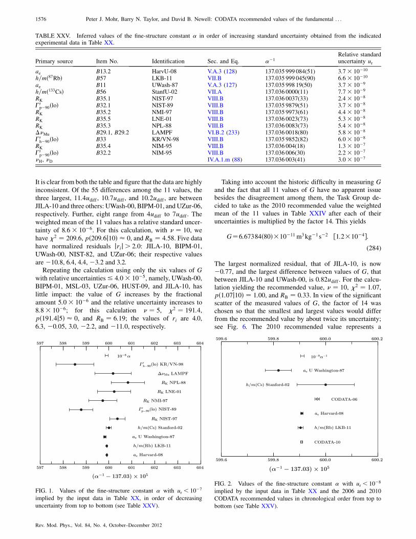
It is clear from both the table and figure that the data are highly
inconsistent. Of the 55 differences among the 11 values, the
three largest, 11:4udiff , 10:7udiff , and 10:2udiff , are between
JILA-10 and three others: UWash-00, BIPM-01, and UZur-06,
respectively. Further, eight range from 4udiff to 7udiff . Theweighted mean of the 11 values has a relative standard uncer-
tainty of 8:6� 10�6. For this calculation, with � ¼ 10, wehave �2 ¼ 209:6, pð209:6j10Þ � 0, and RB ¼ 4:58. Five datahave normalized residuals jrij> 2:0: JILA-10, BIPM-01,
UWash-00, NIST-82, and UZur-06; their respective values
are �10:8, 6.4, 4.4, �3:2 and 3.2.Repeating the calculation using only the six values of G
with relative uncertainties 4:0� 10�5, namely, UWash-00,
BIPM-01, MSL-03, UZur-06, HUST-09, and JILA-10, has
little impact: the value of G increases by the fractional
amount 5:0� 10�6 and the relative uncertainty increases to
8:8� 10�6; for this calculation � ¼ 5, �2 ¼ 191:4,pð191:4j5Þ � 0, and RB ¼ 6:19; the values of ri are 4.0,
6.3, �0:05, 3.0, �2:2, and �11:0, respectively.
Taking into account the historic difficulty in measuring Gand the fact that all 11 values of G have no apparent issuebesides the disagreement among them, the Task Group de-cided to take as the 2010 recommended value the weightedmean of the 11 values in Table XXIV after each of theiruncertainties is multiplied by the factor 14. This yields
G¼6:67384ð80Þ�10�11 m3kg�1 s�2 ½1:2�10�4�:(284)
The largest normalized residual, that of JILA-10, is now�0:77, and the largest difference between values of G, thatbetween JILA-10 and UWash-00, is 0:82udiff . For the calcu-lation yielding the recommended value, � ¼ 10, �2 ¼ 1:07,pð1:07j10Þ ¼ 1:00, and RB ¼ 0:33. In view of the significantscatter of the measured values of G, the factor of 14 waschosen so that the smallest and largest values would differfrom the recommended value by about twice its uncertainty;see Fig. 6. The 2010 recommended value represents a
FIG. 1. Values of the fine-structure constant � with ur < 10�7
implied by the input data in Table XX, in order of decreasing
uncertainty from top to bottom (see Table XXV).
FIG. 2. Values of the fine-structure constant � with ur < 10�8
implied by the input data in Table XX and the 2006 and 2010
CODATA recommended values in chronological order from top to
bottom (see Table XXV).
TABLE XXV. Inferred values of the fine-structure constant � in order of increasing standard uncertainty obtained from the indicatedexperimental data in Table XX.
Primary source Item No. Identification Sec. and Eq. ��1Relative standarduncertainty ur
ae B13:2 HarvU-08 V.A.3 (128) 137.035 999 084(51) 3:7� 10�10
h=mð87RbÞ B57 LKB-11 VII.B 137.035 999 045(90) 6:6� 10�10
ae B11 UWash-87 V.A.3 (127) 137.035 998 19(50) 3:7� 10�9
h=mð133CsÞ B56 StanfU-02 VII.A 137.036 0000(11) 7:7� 10�9
RK B35:1 NIST-97 VIII.B 137.036 0037(33) 2:4� 10�8
�0p�90ðloÞ B32:1 NIST-89 VIII.B 137.035 9879(51) 3:7� 10�8
RK B35:2 NMI-97 VIII.B 137.035 9973(61) 4:4� 10�8
RK B35:5 LNE-01 VIII.B 137.036 0023(73) 5:3� 10�8
RK B35:3 NPL-88 VIII.B 137.036 0083(73) 5:4� 10�8
��Mu B29:1, B29:2 LAMPF VI.B.2 (233) 137.036 0018(80) 5:8� 10�8
�0h�90ðloÞ B33 KR/VN-98 VIII.B 137.035 9852(82) 6:0� 10�8
RK B35:4 NIM-95 VIII.B 137.036 004(18) 1:3� 10�7
�0p�90ðloÞ B32:2 NIM-95 VIII.B 137.036 006(30) 2:2� 10�7
�H, �D IV.A.1.m (88) 137.036 003(41) 3:0� 10�7
1576 Peter J. Mohr, Barry N. Taylor, and David B. Newell: CODATA recommended values of the fundamental . . .
Rev. Mod. Phys., Vol. 84, No. 4, October–December 2012
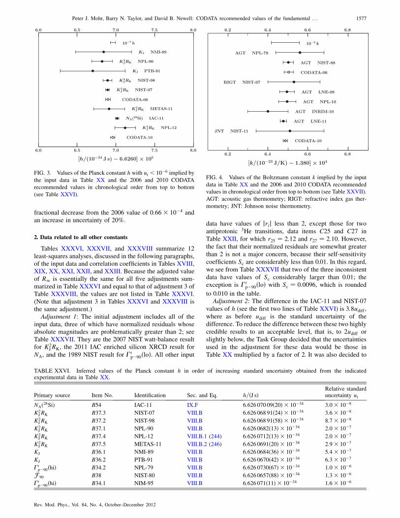
fractional decrease from the 2006 value of 0:66� 10�4 andan increase in uncertainty of 20%.
2. Data related to all other constants
Tables XXXVI, XXXVII, and XXXVIII summarize 12least-squares analyses, discussed in the following paragraphs,of the input data and correlation coefficients in Tables XVIII,XIX, XX, XXI, XXII, and XXIII. Because the adjusted valueof R1 is essentially the same for all five adjustments sum-marized in Table XXXVI and equal to that of adjustment 3 ofTable XXXVIII, the values are not listed in Table XXXVI.(Note that adjustment 3 in Tables XXXVI and XXXVIII isthe same adjustment.)
Adjustment 1: The initial adjustment includes all of theinput data, three of which have normalized residuals whoseabsolute magnitudes are problematically greater than 2; seeTable XXXVII. They are the 2007 NIST watt-balance resultfor K2
JRK, the 2011 IAC enriched silicon XRCD result for
NA, and the 1989 NIST result for �0p�90ðloÞ. All other input
data have values of jrij less than 2, except those for two
antiprotonic 3He transitions, data items C25 and C27 in
Table XXII, for which r25 ¼ 2:12 and r27 ¼ 2:10. However,the fact that their normalized residuals are somewhat greater
than 2 is not a major concern, because their self-sensitivity
coefficients Sc are considerably less than 0.01. In this regard,
we see from Table XXXVII that two of the three inconsistent
data have values of Sc considerably larger than 0.01; the
exception is �0p�90ðloÞ with Sc ¼ 0:0096, which is rounded
to 0.010 in the table.Adjustment 2: The difference in the IAC-11 and NIST-07
values of h (see the first two lines of Table XXVI) is 3:8udiff ,where as before udiff is the standard uncertainty of the
difference. To reduce the difference between these two highly
credible results to an acceptable level, that is, to 2udiff or
slightly below, the Task Group decided that the uncertainties
used in the adjustment for these data would be those in
Table XX multiplied by a factor of 2. It was also decided to
FIG. 3. Values of the Planck constant h with ur < 10�6 implied by
the input data in Table XX and the 2006 and 2010 CODATA
recommended values in chronological order from top to bottom
(see Table XXVI).
FIG. 4. Values of the Boltzmann constant k implied by the input
data in Table XX and the 2006 and 2010 CODATA recommended
values in chronological order from top to bottom (see Table XXVII).
AGT: acoustic gas thermometry; RIGT: refractive index gas ther-
mometry; JNT: Johnson noise thermometry.
TABLE XXVI. Inferred values of the Planck constant h in order of increasing standard uncertainty obtained from the indicatedexperimental data in Table XX.
Primary source Item No. Identification Sec. and Eq. h=ðJ sÞRelative standarduncertainty ur
NA(28Si) B54 IAC-11 IX.F 6:626 070 09ð20Þ � 10�34 3:0� 10�8
K2JRK B37:3 NIST-07 VIII.B 6:626 068 91ð24Þ � 10�34 3:6� 10�8
K2JRK B37:2 NIST-98 VIII.B 6:626 068 91ð58Þ � 10�34 8:7� 10�8
K2JRK B37:1 NPL-90 VIII.B 6:626 0682ð13Þ � 10�34 2:0� 10�7
K2JRK B37:4 NPL-12 VIII.B.1 (244) 6:626 0712ð13Þ � 10�34 2:0� 10�7
K2JRK B37:5 METAS-11 VIII.B.2 (246) 6:626 0691ð20Þ � 10�34 2:9� 10�7
KJ B36:1 NMI-89 VIII.B 6:626 0684ð36Þ � 10�34 5:4� 10�7
KJ B36:2 PTB-91 VIII.B 6:626 0670ð42Þ � 10�34 6:3� 10�7
�0p�90ðhiÞ B34:2 NPL-79 VIII.B 6:626 0730ð67Þ � 10�34 1:0� 10�6
F 90 B38 NIST-80 VIII.B 6:626 0657ð88Þ � 10�34 1:3� 10�6
�0p�90ðhiÞ B34:1 NIM-95 VIII.B 6:626 071ð11Þ � 10�34 1:6� 10�6
Peter J. Mohr, Barry N. Taylor, and David B. Newell: CODATA recommended values of the fundamental . . . 1577
Rev. Mod. Phys., Vol. 84, No. 4, October–December 2012
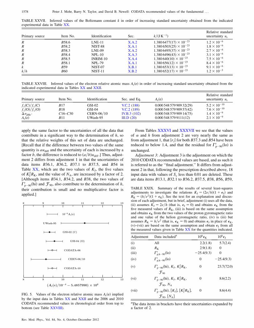
apply the same factor to the uncertainties of all the data that
contribute in a significant way to the determination of h, sothat the relative weights of this set of data are unchanged.
[Recall that if the difference between two values of the same
quantity is audiff and the uncertainty of each is increased by afactor b, the difference is reduced to ða=bÞudiff .] Thus, adjust-ment 2 differs from adjustment 1 in that the uncertainties of
data items B36:1, B36:2, B37:1 to B37:5, and B54 in
Table XX, which are the two values of KJ, the five values
of K2JRK, and the value of NA, are increased by a factor of 2.
[Although items B34:1, B34:2, and B38, the two values of
�0p�90ðhiÞ and F 90, also contribute to the determination of h,
their contribution is small and no multiplicative factor is
applied.]
From Tables XXXVI and XXXVII we see that the valuesof � and h from adjustment 2 are very nearly the same asfrom adjustment 1, that jrij for both B37:3 and B54 have beenreduced to below 1.4, and that the residual for �0
p�90ðloÞ isunchanged.
Adjustment 3: Adjustment 3 is the adjustment on which the2010 CODATA recommended values are based, and as such itis referred to as the ‘‘final adjustment.’’ It differs from adjust-ment 2 in that, following the prescription described above, 18input data with values of Sc less than 0.01 are deleted. Theseare data items B13:1, B32:1 to B36:2, B37:5, B38, B56, B59,
TABLE XXVIII. Inferred values of the electron relative atomic mass ArðeÞ in order of increasing standard uncertainty obtained from theindicated experimental data in Tables XX and XXII.
Primary source Item No. Identification Sec. and Eq. ArðeÞRelative standarduncertainty ur
fsðCÞ=fcðCÞ B17 GSI-02 V.C.2 (188) 0.000 548 579 909 32(29) 5:2� 10�10
fsðOÞ=fcðOÞ B18 GSI-04 V.C.2 (189) 0.000 548 579 909 57(42) 7:6� 10�10
���pHeþ C16–C30 CERN-06=10 IV.B.3 (102) 0.000 548 579 909 14(75) 1:4� 10�9
ArðeÞ B11 UWash-95 III.D (20) 0.000 548 579 9111(12) 2:1� 10�9
FIG. 5. Values of the electron relative atomic mass ArðeÞ implied
by the input data in Tables XX and XXII and the 2006 and 2010
CODATA recommended values in chronological order from top to
bottom (see Table XXVIII).
TABLE XXIX. Summary of the results of several least-squaresadjustments to investigate the relations KJ ¼ ð2e=hÞð1þ �JÞ andRK ¼ ðh=e2Þð1þ �KÞ. See the text for an explanation and discus-sion of each adjustment, but in brief, adjustment (i) uses all the data,(ii) assumes KJ ¼ 2e=h (that is, �J ¼ 0) and obtains �K from thefive measured values of RK, (iii) is based on the same assumptionand obtains �K from the two values of the proton gyromagnetic ratioand one value of the helion gyromagnetic ratio, (iv) is (iii) butassumes RK ¼ h=e2 (that is, �K ¼ 0) and obtains �J in place of �K,(v)–(vii) are based on the same assumption and obtain �J from allthe measured values given in Table XX for the quantities indicated.
Adjustment Data includeda 108�K 108�J
(i) All 2.2(1.8) 5.7(2.4)
(ii) RK 2.9(1.8) 0
(iii) �0p;h�90ðloÞ �25:4ð9:3Þ 0
(iv) �0p;h�90ðloÞ 0 �25:4ð9:3Þ
(v) �0p�90ðhiÞ, KJ, K
2JRK,
F 90
0 23.7(72.0)
(vi) �0p�90ðhiÞ, KJ, K
2JRK,
F 90, NA
0 8.6(2.2)
(vii) �0p�90ðhiÞ, ½KJ�, ½K2
JRK�,F 90, ½NA�
0 8.6(4.4)
aThe data items in brackets have their uncertainties expanded bya factor of 2.
TABLE XXVII. Inferred values of the Boltzmann constant k in order of increasing standard uncertainty obtained from the indicatedexperimental data in Table XX.
Primary source Item No. Identification Sec. k=ðJK�1ÞRelative standarduncertainty ur
R B58:6 LNE-11 X.A.2 1:380 6477ð17Þ � 10�23 1:2� 10�6
R B58:2 NIST-88 X.A.1 1:380 6503ð25Þ � 10�23 1:8� 10�6
R B58:3 LNE-09 X.A.2 1:380 6495ð37Þ � 10�23 2:7� 10�6
R B58:4 NPL-10 X.A.3 1:380 6496ð43Þ � 10�23 3:1� 10�6
R B58:5 INRIM-10 X.A.4 1:380 640ð10Þ � 10�23 7:5� 10�6
R B58:1 NPL-79 X.A.1 1:380 656ð12Þ � 10�23 8:4� 10�6
k B59 NIST-07 X.B.1 1:380 653ð13Þ � 10�23 9:1� 10�6
k=h B60 NIST-11 X.B.2 1:380 652ð17Þ � 10�23 1:2� 10�5
1578 Peter J. Mohr, Barry N. Taylor, and David B. Newell: CODATA recommended values of the fundamental . . .
Rev. Mod. Phys., Vol. 84, No. 4, October–December 2012
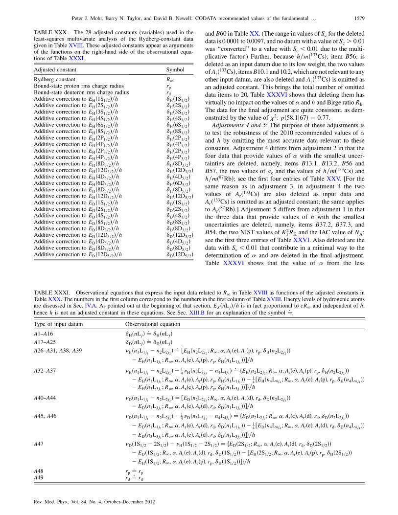
and B60 in Table XX. (The range in values of Sc for the deleteddata is 0.0001 to 0.0097, and no datumwith a value ofSc > 0:01was ‘‘converted’’ to a value with Sc < 0:01 due to the multi-
plicative factor.) Further, because h=mð133CsÞ, item B56, isdeleted as an input datum due to its low weight, the two values
ofArð133CsÞ, itemsB10:1 and 10.2,which are not relevant to anyother input datum, are also deleted and Arð133CsÞ is omitted as
an adjusted constant. This brings the total number of omitted
data items to 20. Table XXXVI shows that deleting them has
virtually no impact on the values of� and h and Birge ratioRB.
The data for the final adjustment are quite consistent, as dem-
onstrated by the value of �2: pð58:1j67Þ ¼ 0:77.Adjustments 4 and 5: The purpose of these adjustments is
to test the robustness of the 2010 recommended values of �and h by omitting the most accurate data relevant to these
constants. Adjustment 4 differs from adjustment 2 in that the
four data that provide values of � with the smallest uncer-
tainties are deleted, namely, items B13:1, B13:2, B56 and
B57, the two values of ae and the values of h=mð133CsÞ andh=mð87RbÞ; see the first four entries of Table XXV. [For the
same reason as in adjustment 3, in adjustment 4 the two
values of Arð133CsÞ are also deleted as input data and
Arð133CsÞ is omitted as an adjusted constant; the same applies
to Arð87RbÞ.] Adjustment 5 differs from adjustment 1 in that
the three data that provide values of h with the smallest
uncertainties are deleted, namely, items B37:2, B37:3, andB54, the two NIST values of K2
JRK and the IAC value of NA;
see the first three entries of Table XXVI. Also deleted are the
data with Sc < 0:01 that contribute in a minimal way to the
determination of � and are deleted in the final adjustment.
Table XXXVI shows that the value of � from the less
TABLE XXX. The 28 adjusted constants (variables) used in theleast-squares multivariate analysis of the Rydberg-constant datagiven in Table XVIII. These adjusted constants appear as argumentsof the functions on the right-hand side of the observational equa-tions of Table XXXI.
Adjusted constant Symbol
Rydberg constant R1Bound-state proton rms charge radius rpBound-state deuteron rms charge radius rdAdditive correction to EHð1S1=2Þ=h �Hð1S1=2ÞAdditive correction to EHð2S1=2Þ=h �Hð2S1=2ÞAdditive correction to EHð3S1=2Þ=h �Hð3S1=2ÞAdditive correction to EHð4S1=2Þ=h �Hð4S1=2ÞAdditive correction to EHð6S1=2Þ=h �Hð6S1=2ÞAdditive correction to EHð8S1=2Þ=h �Hð8S1=2ÞAdditive correction to EHð2P1=2Þ=h �Hð2P1=2ÞAdditive correction to EHð4P1=2Þ=h �Hð4P1=2ÞAdditive correction to EHð2P3=2Þ=h �Hð2P3=2ÞAdditive correction to EHð4P3=2Þ=h �Hð4P3=2ÞAdditive correction to EHð8D3=2Þ=h �Hð8D3=2ÞAdditive correction to EHð12D3=2Þ=h �Hð12D3=2ÞAdditive correction to EHð4D5=2Þ=h �Hð4D5=2ÞAdditive correction to EHð6D5=2Þ=h �Hð6D5=2ÞAdditive correction to EHð8D5=2Þ=h �Hð8D5=2ÞAdditive correction to EHð12D5=2Þ=h �Hð12D5=2ÞAdditive correction to EDð1S1=2Þ=h �Dð1S1=2ÞAdditive correction to EDð2S1=2Þ=h �Dð2S1=2ÞAdditive correction to EDð4S1=2Þ=h �Dð4S1=2ÞAdditive correction to EDð8S1=2Þ=h �Dð8S1=2ÞAdditive correction to EDð8D3=2Þ=h �Dð8D3=2ÞAdditive correction to EDð12D3=2Þ=h �Dð12D3=2ÞAdditive correction to EDð4D5=2Þ=h �Dð4D5=2ÞAdditive correction to EDð8D5=2Þ=h �Dð8D5=2ÞAdditive correction to EDð12D5=2Þ=h �Dð12D5=2Þ
TABLE XXXI. Observational equations that express the input data related to R1 in Table XVIII as functions of the adjusted constants inTable XXX. The numbers in the first column correspond to the numbers in the first column of Table XVIII. Energy levels of hydrogenic atomsare discussed in Sec. IV.A. As pointed out at the beginning of that section, EXðnLjÞ=h is in fact proportional to cR1 and independent of h,hence h is not an adjusted constant in these equations. See Sec. XIII.B for an explanation of the symbol ¼: .Type of input datum Observational equation
A1–A16 �HðnLjÞ ¼: �HðnLjÞA17–A25 �DðnLjÞ ¼: �DðnLjÞA26–A31, A38, A39 �Hðn1L1j1 � n2L2j2 Þ ¼
: ½EHðn2L2j2 ;R1; �; ArðeÞ; ArðpÞ; rp; �Hðn2L2j2 ÞÞ� EHðn1L1j1 ;R1; �; ArðeÞ; ArðpÞ; rp; �Hðn1L1j1 ÞÞ�=h
A32–A37 �Hðn1L1j1 � n2L2j2 Þ � 14�Hðn3L3j3 � n4L4j4 Þ ¼
: fEHðn2L2j2 ;R1; �; ArðeÞ; ArðpÞ; rp; �Hðn2L2j2 ÞÞ� EHðn1L1j1 ;R1; �; ArðeÞ; ArðpÞ; rp; �Hðn1L1j1 ÞÞ � 1
4 ½EHðn4L4j4 ;R1; �; ArðeÞ; ArðpÞ; rp; �Hðn4L4j4 ÞÞ� EHðn3L3j3 ;R1; �; ArðeÞ; ArðpÞ; rp; �Hðn3L3j3 ÞÞ�g=h
A40–A44 �Dðn1L1j1 � n2L2j2 Þ ¼: ½EDðn2L2j2 ;R1; �; ArðeÞ; ArðdÞ; rd; �Dðn2L2j2 ÞÞ
� EDðn1L1j1 ;R1; �; ArðeÞ; ArðdÞ; rd; �Dðn1L1j1 ÞÞ�=hA45, A46 �Dðn1L1j1 � n2L2j2 Þ � 1
4�Dðn3L3j3 � n4L4j4 Þ ¼: fEDðn2L2j2 ;R1; �; ArðeÞ; ArðdÞ; rd; �Dðn2L2j2 ÞÞ
� EDðn1L1j1 ;R1; �; ArðeÞ; ArðdÞ; rd; �Dðn1L1j1 ÞÞ � 14 ½EDðn4L4j4 ;R1; �; ArðeÞ; ArðdÞ; rd; �Dðn4L4j4 ÞÞ
� EDðn3L3j3 ;R1; �; ArðeÞ; ArðdÞ; rd; �Dðn3L3j3 ÞÞ�g=hA47 �Dð1S1=2 � 2S1=2Þ � �Hð1S1=2 � 2S1=2Þ ¼: fEDð2S1=2;R1; �; ArðeÞ; ArðdÞ; rd; �Dð2S1=2ÞÞ
� EDð1S1=2;R1; �; ArðeÞ; ArðdÞ; rd; �Dð1S1=2ÞÞ � ½EHð2S1=2;R1; �; ArðeÞ; ArðpÞ; rp; �Hð2S1=2ÞÞ� EHð1S1=2;R1; �; ArðeÞ; ArðpÞ; rp; �Hð1S1=2ÞÞ�g=h
A48 rp ¼: rpA49 rd ¼: rd
Peter J. Mohr, Barry N. Taylor, and David B. Newell: CODATA recommended values of the fundamental . . . 1579
Rev. Mod. Phys., Vol. 84, No. 4, October–December 2012
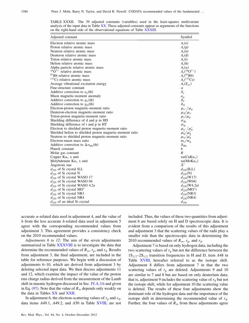
accurate �-related data used in adjustment 4, and the value of
h from the less accurate h-related data used in adjustment 5
agree with the corresponding recommended values from
adjustment 3. This agreement provides a consistency check
on the 2010 recommended values.Adjustments 6 to 12: The aim of the seven adjustments
summarized in Table XXXVIII is to investigate the data that
determine the recommended values of R1, rp, and rd. Resultsfrom adjustment 3, the final adjustment, are included in the
table for reference purposes. We begin with a discussion of
adjustments 6–10, which are derived from adjustment 3 by
deleting selected input data. We then discuss adjustments 11
and 12, which examine the impact of the value of the proton
rms charge radius derived from the measurement of the Lamb
shift in muonic hydrogen discussed in Sec. IV.A.3.b and given
in Eq. (97). Note that the value of R1 depends only weakly on
the data in Tables XX and XXII.In adjustment 6, the electron-scattering values of rp and rd,
data items A49:1, A49:2, and A50 in Table XVIII, are not
included. Thus, the values of these two quantities from adjust-
ment 6 are based solely on H and D spectroscopic data. It is
evident from a comparison of the results of this adjustment
and adjustment 3 that the scattering values of the radii play a
smaller role than the spectroscopic data in determining the
2010 recommended values of R1, rp, and rd.
Adjustment 7 is based on only hydrogen data, including thetwo scattering values of rp but not the difference between the
1S1=2–2S1=2 transition frequencies in H and D, item A48 in
Table XVIII, hereafter referred to as the isotope shift.Adjustment 8 differs from adjustment 7 in that the twoscattering values of rp are deleted. Adjustments 9 and 10
are similar to 7 and 8 but are based on only deuterium data;that is, adjustment 9 includes the scattering value of rd but notthe isotope shift, while for adjustment 10 the scattering valueis deleted. The results of these four adjustments show thedominant role of the hydrogen data and the importance of theisotope shift in determining the recommended value of rd.Further, the four values of R1 from these adjustments agree
TABLE XXXII. The 39 adjusted constants (variables) used in the least-squares multivariateanalysis of the input data in Table XX. These adjusted constants appear as arguments of the functionson the right-hand side of the observational equations of Table XXXIII.
Adjusted constant Symbol
Electron relative atomic mass ArðeÞProton relative atomic mass ArðpÞNeutron relative atomic mass ArðnÞDeuteron relative atomic mass ArðdÞTriton relative atomic mass ArðtÞHelion relative atomic mass ArðhÞAlpha particle relative atomic mass Arð�Þ16O7þ relative atomic mass Arð16O7þÞ87Rb relative atomic mass Arð87RbÞ133Cs relative atomic mass Arð133CsÞAverage vibrational excitation energy ArðEavÞFine-structure constant �Additive correction to aeðthÞ �e
Muon magnetic-moment anomaly a�Additive correction to gCðthÞ �C
Additive correction to gOðthÞ �O
Electron-proton magnetic-moment ratio �e�=�p
Deuteron-electron magnetic-moment ratio �d=�e�
Triton-proton magnetic-moment ratio �t=�p
Shielding difference of d and p in HD �dp
Shielding difference of t and p in HT �tp
Electron to shielded proton magnetic-moment ratio �e�=�0p
Shielded helion to shielded proton magnetic-moment ratio �0h=�
0p
Neutron to shielded proton magnetic-moment ratio �n=�0p
Electron-muon mass ratio me=m�
Additive correction to ��MuðthÞ �Mu
Planck constant hMolar gas constant RCopper K�1 x unit xuðCuK�1ÞMolybdenum K�1 x unit xuðMoK�1ÞAngstrom star �A�d220 of Si crystal ILL d220ðILLÞd220 of Si crystal N d220ðNÞd220 of Si crystal WASO 17 d220ðW17Þd220 of Si crystal WASO 04 d220ðW04Þd220 of Si crystal WASO 4.2a d220ðW4:2aÞd220 of Si crystal MO� d220ðMO�Þd220 of Si crystal NR3 d220ðNR3Þd220 of Si crystal NR4 d220ðNR4Þd220 of an ideal Si crystal d220
1580 Peter J. Mohr, Barry N. Taylor, and David B. Newell: CODATA recommended values of the fundamental . . .
Rev. Mod. Phys., Vol. 84, No. 4, October–December 2012
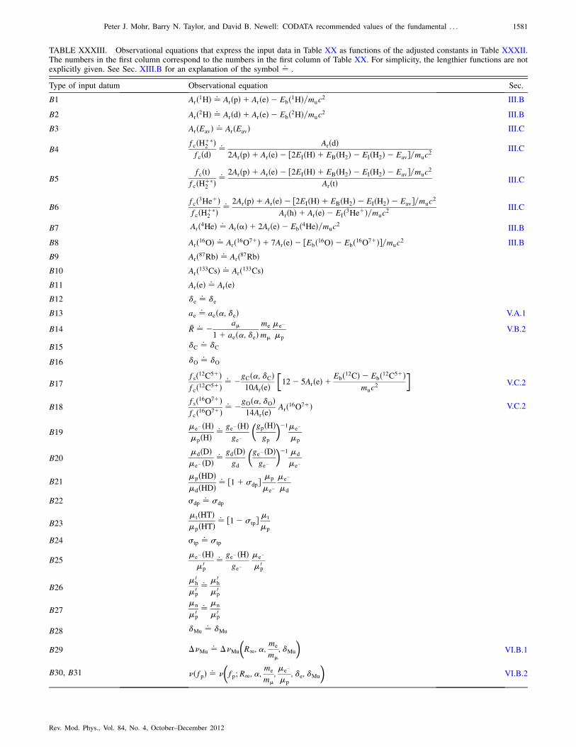
TABLE XXXIII. Observational equations that express the input data in Table XX as functions of the adjusted constants in Table XXXII.The numbers in the first column correspond to the numbers in the first column of Table XX. For simplicity, the lengthier functions are notexplicitly given. See Sec. XIII.B for an explanation of the symbol ¼: .
Type of input datum Observational equation Sec.
B1 Arð1HÞ ¼: ArðpÞ þ ArðeÞ � Ebð1HÞ=muc2 III.B
B2 Arð2HÞ ¼: ArðdÞ þ ArðeÞ � Ebð2HÞ=muc2 III.B
B3 ArðEavÞ ¼: ArðEavÞ III.C
B4fcðHþ�
2 ÞfcðdÞ ¼: ArðdÞ
2ArðpÞ þ ArðeÞ � ½2EIðHÞ þ EBðH2Þ � EIðH2Þ � Eav�=muc2
III.C
B5fcðtÞ
fcðHþ�2 Þ ¼
: 2ArðpÞ þ ArðeÞ � ½2EIðHÞ þ EBðH2Þ � EIðH2Þ � Eav�=muc2
ArðtÞ III.C
B6fcð3HeþÞfcðHþ�
2 Þ ¼: 2ArðpÞ þ ArðeÞ � ½2EIðHÞ þ EBðH2Þ � EIðH2Þ � Eav�=muc2
ArðhÞ þ ArðeÞ � EIð3HeþÞ=muc2 III.C
B7 Arð4HeÞ ¼: Arð�Þ þ 2ArðeÞ � Ebð4HeÞ=muc2
III.B
B8 Arð16OÞ ¼: Arð16O7þÞ þ 7ArðeÞ � ½Ebð16OÞ � Ebð16O7þÞ�=muc2 III.B
B9 Arð87RbÞ ¼: Arð87RbÞB10 Arð133CsÞ ¼: Arð133CsÞB11 ArðeÞ ¼: ArðeÞB12 �e ¼: �e
B13 ae ¼: aeð�; �eÞ V.A.1
B14 �R ¼: � a�1þ aeð�; �eÞ
me
m�
�e�
�p
V.B.2
B15 �C ¼: �C
B16 �O ¼: �O
B17fsð12C5þÞfcð12C5þÞ ¼
: �gCð�; �CÞ10ArðeÞ
�12� 5ArðeÞ þ Ebð12CÞ � Ebð12C5þÞ
muc2
�V.C.2
B18fsð16O7þÞfcð16O7þÞ ¼
: �gOð�; �OÞ14ArðeÞ Arð16O7þÞ V.C.2
B19�e�ðHÞ�pðHÞ ¼: ge�ðHÞ
ge�
�gpðHÞgp
��1�e�
�p
B20�dðDÞ�e�ðDÞ ¼
: gdðDÞgd
�ge� ðDÞge�
��1 �d
�e�
B21�pðHDÞ�dðHDÞ ¼
: ½1þ �dp��p
�e�
�e�
�d
B22 �dp ¼: �dp
B23�tðHTÞ�pðHTÞ ¼
: ½1� �tp� �t
�p
B24 �tp ¼: �tp
B25�e�ðHÞ�0
p
¼: ge�ðHÞge�
�e�
�0p
B26�0
h
�0p
¼: �0h
�0p
B27�n
�0p
¼: �n
�0p
B28 �Mu ¼: �Mu
B29 ��Mu ¼: ��Mu
�R1; �;
me
m�
; �Mu
�VI.B.1
B30, B31 �ðfpÞ ¼: �
�fp;R1; �;
me
m�
;�e�
�p
; �e; �Mu
�VI.B.2
Peter J. Mohr, Barry N. Taylor, and David B. Newell: CODATA recommended values of the fundamental . . . 1581
Rev. Mod. Phys., Vol. 84, No. 4, October–December 2012
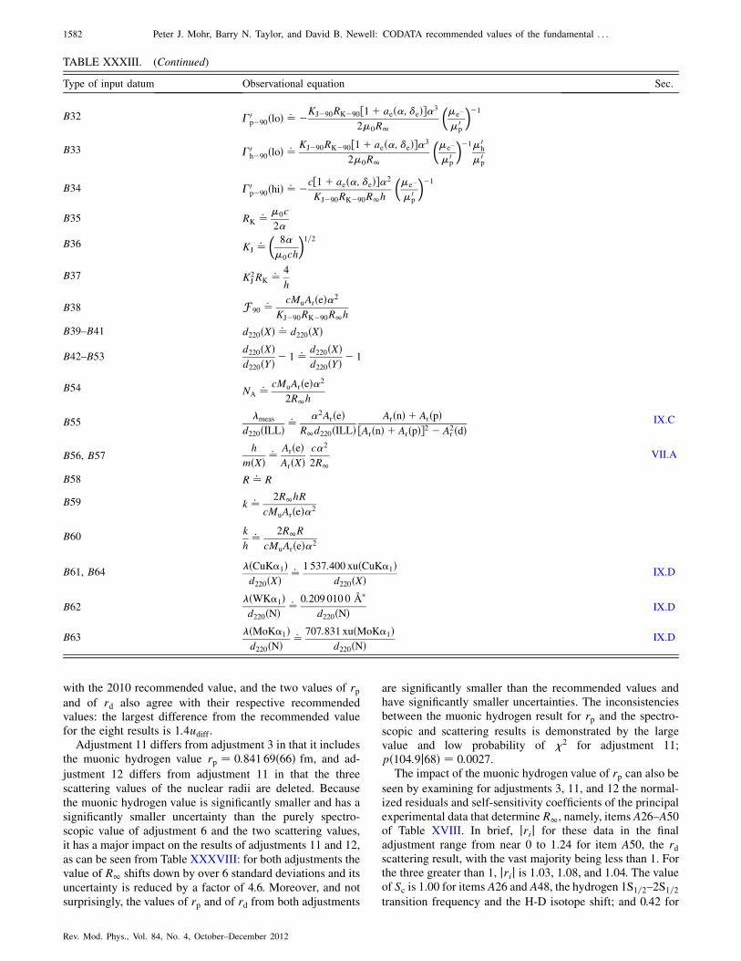
with the 2010 recommended value, and the two values of rpand of rd also agree with their respective recommendedvalues: the largest difference from the recommended valuefor the eight results is 1:4udiff .
Adjustment 11 differs from adjustment 3 in that it includesthe muonic hydrogen value rp ¼ 0:841 69ð66Þ fm, and ad-
justment 12 differs from adjustment 11 in that the three
scattering values of the nuclear radii are deleted. Because
the muonic hydrogen value is significantly smaller and has a
significantly smaller uncertainty than the purely spectro-
scopic value of adjustment 6 and the two scattering values,
it has a major impact on the results of adjustments 11 and 12,
as can be seen from Table XXXVIII: for both adjustments thevalue of R1 shifts down by over 6 standard deviations and its
uncertainty is reduced by a factor of 4.6. Moreover, and not
surprisingly, the values of rp and of rd from both adjustments
are significantly smaller than the recommended values andhave significantly smaller uncertainties. The inconsistenciesbetween the muonic hydrogen result for rp and the spectro-
scopic and scattering results is demonstrated by the largevalue and low probability of �2 for adjustment 11;pð104:9j68Þ ¼ 0:0027.
The impact of the muonic hydrogen value of rp can also be
seen by examining for adjustments 3, 11, and 12 the normal-ized residuals and self-sensitivity coefficients of the principalexperimental data that determine R1, namely, items A26–A50of Table XVIII. In brief, jrij for these data in the finaladjustment range from near 0 to 1.24 for item A50, the rdscattering result, with the vast majority being less than 1. Forthe three greater than 1, jrij is 1.03, 1.08, and 1.04. The valueof Sc is 1.00 for items A26 and A48, the hydrogen 1S1=2–2S1=2transition frequency and the H-D isotope shift; and 0.42 for
Type of input datum Observational equation Sec.
B32 �0p�90ðloÞ ¼: �KJ�90RK�90½1þ aeð�; �eÞ��3
2�0R1
��e�
�0p
��1
B33 �0h�90ðloÞ ¼
: KJ�90RK�90½1þ aeð�; �eÞ��3
2�0R1
��e�
�0p
��1�0h
�0p
B34 �0p�90ðhiÞ ¼: �c½1þ aeð�; �eÞ��2
KJ�90RK�90R1h
��e�
�0p
��1
B35 RK ¼: �0c
2�
B36 KJ ¼:�
8�
�0ch
�1=2
B37 K2JRK ¼: 4
h
B38 F 90 ¼: cMuArðeÞ�2
KJ�90RK�90R1hB39–B41 d220ðXÞ ¼: d220ðXÞ
B42–B53d220ðXÞd220ðYÞ � 1 ¼: d220ðXÞ
d220ðYÞ � 1
B54 NA ¼: cMuArðeÞ�2
2R1h
B55meas
d220ðILLÞ ¼: �2ArðeÞR1d220ðILLÞ
ArðnÞ þ ArðpÞ½ArðnÞ þ ArðpÞ�2 � A2
r ðdÞIX.C
B56, B57h
mðXÞ ¼: ArðeÞArðXÞ
c�2
2R1VII.A
B58 R ¼: R
B59 k ¼: 2R1hRcMuArðeÞ�2
B60k
h¼: 2R1R
cMuArðeÞ�2
B61, B64ðCuK�1Þd220ðXÞ ¼: 1 537:400 xuðCuK�1Þ
d220ðXÞIX.D
B62ðWK�1Þd220ðNÞ ¼: 0:209 010 0 �A�
d220ðNÞ IX.D
B63ðMoK�1Þd220ðNÞ ¼: 707:831 xuðMoK�1Þ
d220ðNÞIX.D
TABLE XXXIII. (Continued)
1582 Peter J. Mohr, Barry N. Taylor, and David B. Newell: CODATA recommended values of the fundamental . . .
Rev. Mod. Phys., Vol. 84, No. 4, October–December 2012
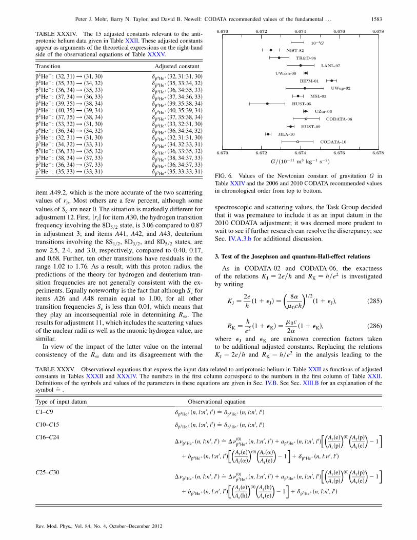
item A49:2, which is the more accurate of the two scattering
values of rp. Most others are a few percent, although some
values of Sc are near 0. The situation is markedly different for
adjustment 12. First, jrij for item A30, the hydrogen transitionfrequency involving the 8D5=2 state, is 3.06 compared to 0.87
in adjustment 3; and items A41, A42, and A43, deuteriumtransitions involving the 8S1=2, 8D3=2, and 8D5=2 states, are
now 2.5, 2.4, and 3.0, respectively, compared to 0.40, 0.17,
and 0.68. Further, ten other transitions have residuals in the
range 1.02 to 1.76. As a result, with this proton radius, the
predictions of the theory for hydrogen and deuterium tran-
sition frequencies are not generally consistent with the ex-
periments. Equally noteworthy is the fact that although Sc foritems A26 and A48 remain equal to 1.00, for all other
transition frequencies Sc is less than 0.01, which means that
they play an inconsequential role in determining R1. Theresults for adjustment 11, which includes the scattering values
of the nuclear radii as well as the muonic hydrogen value, are
similar.In view of the impact of the latter value on the internal
consistency of the R1 data and its disagreement with the
spectroscopic and scattering values, the Task Group decidedthat it was premature to include it as an input datum in the2010 CODATA adjustment; it was deemed more prudent towait to see if further research can resolve the discrepancy; seeSec. IV.A.3.b for additional discussion.
3. Test of the Josephson and quantum-Hall-effect relations
As in CODATA-02 and CODATA-06, the exactnessof the relations KJ ¼ 2e=h and RK ¼ h=e2 is investigatedby writing
KJ ¼ 2e
hð1þ �JÞ ¼
�8�
�0ch
�1=2ð1þ �JÞ; (285)
RK ¼ h
e2ð1þ �KÞ ¼ �0c
2�ð1þ �KÞ; (286)
where �J and �K are unknown correction factors takento be additional adjusted constants. Replacing the relationsKJ ¼ 2e=h and RK ¼ h=e2 in the analysis leading to the
TABLE XXXV. Observational equations that express the input data related to antiprotonic helium in Table XXII as functions of adjustedconstants in Tables XXXII and XXXIV. The numbers in the first column correspond to the numbers in the first column of Table XXII.Definitions of the symbols and values of the parameters in these equations are given in Sec. IV.B. See Sec. XIII.B for an explanation of thesymbol ¼: .
Type of input datum Observational equation
C1–C9 ��p4Heþ ðn; l:n0; l0Þ ¼: ��p4Heþðn; l:n0; l0ÞC10–C15 ��p3Heþ ðn; l:n0; l0Þ ¼: ��p3Heþðn; l:n0; l0ÞC16–C24
���p4Heþ ðn; l:n0; l0Þ ¼: ��ð0Þ�p4Heþðn; l:n0; l0Þ þ a�p4Heþ ðn; l:n0; l0Þ
��ArðeÞArðpÞ
�ð0Þ�ArðpÞArðeÞ
�� 1
�
þ b�p4Heþ ðn; l:n0; l0Þ��
ArðeÞArð�Þ
�ð0Þ�Arð�ÞArðeÞ
�� 1
�þ ��p4Heþ ðn; l:n0; l0Þ
C25–C30���p3Heþ ðn; l:n0; l0Þ ¼: ��ð0Þ
�p3Heþðn; l:n0; l0Þ þ a�p3Heþ ðn; l:n0; l0Þ��
ArðeÞArðpÞ
�ð0Þ�ArðpÞArðeÞ
�� 1
�
þ b�p3Heþ ðn; l:n0; l0Þ��
ArðeÞArðhÞ
�ð0Þ�ArðhÞArðeÞ
�� 1
�þ ��p3Heþðn; l:n0; l0Þ
FIG. 6. Values of the Newtonian constant of gravitation G in
Table XXIV and the 2006 and 2010 CODATA recommended values
in chronological order from top to bottom.
TABLE XXXIV. The 15 adjusted constants relevant to the anti-protonic helium data given in Table XXII. These adjusted constantsappear as arguments of the theoretical expressions on the right-handside of the observational equations of Table XXXV.
Transition Adjusted constant
�p4Heþ: ð32; 31Þ ! ð31; 30Þ ��p4Heþ ð32; 31:31; 30Þ�p4Heþ: ð35; 33Þ ! ð34; 32Þ ��p4Heþ ð35; 33:34; 32Þ�p4Heþ: ð36; 34Þ ! ð35; 33Þ ��p4Heþ ð36; 34:35; 33Þ�p4Heþ: ð37; 34Þ ! ð36; 33Þ ��p4Heþ ð37; 34:36; 33Þ�p4Heþ: ð39; 35Þ ! ð38; 34Þ ��p4Heþ ð39; 35:38; 34Þ�p4Heþ: ð40; 35Þ ! ð39; 34Þ ��p4Heþ ð40; 35:39; 34Þ�p4Heþ: ð37; 35Þ ! ð38; 34Þ ��p4Heþ ð37; 35:38; 34Þ�p4Heþ: ð33; 32Þ ! ð31; 30Þ ��p4Heþ ð33; 32:31; 30Þ�p4Heþ: ð36; 34Þ ! ð34; 32Þ ��p4Heþ ð36; 34:34; 32Þ�p3Heþ: ð32; 31Þ ! ð31; 30Þ ��p3Heþ ð32; 31:31; 30Þ�p3Heþ: ð34; 32Þ ! ð33; 31Þ ��p3Heþ ð34; 32:33; 31Þ�p3Heþ: ð36; 33Þ ! ð35; 32Þ ��p3Heþ ð36; 33:35; 32Þ�p3Heþ: ð38; 34Þ ! ð37; 33Þ ��p3Heþ ð38; 34:37; 33Þ�p3Heþ: ð36; 34Þ ! ð37; 33Þ ��p3Heþ ð36; 34:37; 33Þ�p3Heþ: ð35; 33Þ ! ð33; 31Þ ��p3Heþ ð35; 33:33; 31Þ
Peter J. Mohr, Barry N. Taylor, and David B. Newell: CODATA recommended values of the fundamental . . . 1583
Rev. Mod. Phys., Vol. 84, No. 4, October–December 2012
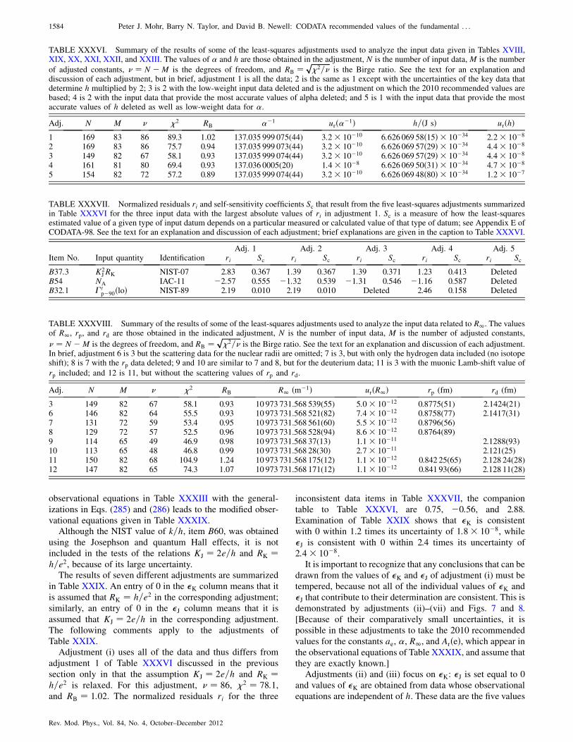
observational equations in Table XXXIII with the general-
izations in Eqs. (285) and (286) leads to the modified obser-
vational equations given in Table XXXIX.Although the NIST value of k=h, item B60, was obtained
using the Josephson and quantum Hall effects, it is not
included in the tests of the relations KJ ¼ 2e=h and RK ¼h=e2, because of its large uncertainty.
The results of seven different adjustments are summarized
in Table XXIX. An entry of 0 in the �K column means that it
is assumed that RK ¼ h=e2 in the corresponding adjustment;
similarly, an entry of 0 in the �J column means that it is
assumed that KJ ¼ 2e=h in the corresponding adjustment.
The following comments apply to the adjustments of
Table XXIX.Adjustment (i) uses all of the data and thus differs from
adjustment 1 of Table XXXVI discussed in the previous
section only in that the assumption KJ ¼ 2e=h and RK ¼h=e2 is relaxed. For this adjustment, � ¼ 86, �2 ¼ 78:1,and RB ¼ 1:02. The normalized residuals ri for the three
inconsistent data items in Table XXXVII, the companion
table to Table XXXVI, are 0.75, �0:56, and 2.88.
Examination of Table XXIX shows that �K is consistent
with 0 within 1.2 times its uncertainty of 1:8� 10�8, while
�J is consistent with 0 within 2.4 times its uncertainty of
2:4� 10�8.It is important to recognize that any conclusions that can be
drawn from the values of �K and �J of adjustment (i) must be
tempered, because not all of the individual values of �K and
�J that contribute to their determination are consistent. This is
demonstrated by adjustments (ii)–(vii) and Figs. 7 and 8.
[Because of their comparatively small uncertainties, it is
possible in these adjustments to take the 2010 recommended
values for the constants ae, �, R1, and ArðeÞ, which appear inthe observational equations of Table XXXIX, and assume that
they are exactly known.]Adjustments (ii) and (iii) focus on �K: �J is set equal to 0
and values of �K are obtained from data whose observational
equations are independent of h. These data are the five values
TABLE XXXVI. Summary of the results of some of the least-squares adjustments used to analyze the input data given in Tables XVIII,XIX, XX, XXI, XXII, and XXIII. The values of � and h are those obtained in the adjustment, N is the number of input data, M is the number
of adjusted constants, � ¼ N �M is the degrees of freedom, and RB ¼ ffiffiffiffiffiffiffiffiffiffiffi�2=�
pis the Birge ratio. See the text for an explanation and
discussion of each adjustment, but in brief, adjustment 1 is all the data; 2 is the same as 1 except with the uncertainties of the key data thatdetermine h multiplied by 2; 3 is 2 with the low-weight input data deleted and is the adjustment on which the 2010 recommended values arebased; 4 is 2 with the input data that provide the most accurate values of alpha deleted; and 5 is 1 with the input data that provide the mostaccurate values of h deleted as well as low-weight data for �.
Adj. N M � �2 RB ��1 urð��1Þ h=ðJ sÞ urðhÞ1 169 83 86 89.3 1.02 137.035 999 075(44) 3:2� 10�10 6:626 069 58ð15Þ � 10�34 2:2� 10�8
2 169 83 86 75.7 0.94 137.035 999 073(44) 3:2� 10�10 6:626 069 57ð29Þ � 10�34 4:4� 10�8
3 149 82 67 58.1 0.93 137.035 999 074(44) 3:2� 10�10 6:626 069 57ð29Þ � 10�34 4:4� 10�8
4 161 81 80 69.4 0.93 137.036 0005(20) 1:4� 10�8 6:626 069 50ð31Þ � 10�34 4:7� 10�8
5 154 82 72 57.2 0.89 137.035 999 074(44) 3:2� 10�10 6:626 069 48ð80Þ � 10�34 1:2� 10�7
TABLE XXXVII. Normalized residuals ri and self-sensitivity coefficients Sc that result from the five least-squares adjustments summarizedin Table XXXVI for the three input data with the largest absolute values of ri in adjustment 1. Sc is a measure of how the least-squaresestimated value of a given type of input datum depends on a particular measured or calculated value of that type of datum; see Appendix E ofCODATA-98. See the text for an explanation and discussion of each adjustment; brief explanations are given in the caption to Table XXXVI.
Adj. 1 Adj. 2 Adj. 3 Adj. 4 Adj. 5Item No. Input quantity Identification ri Sc ri Sc ri Sc ri Sc ri Sc
B37:3 K2JRK NIST-07 2.83 0.367 1.39 0.367 1.39 0.371 1.23 0.413 Deleted
B54 NA IAC-11 �2:57 0.555 �1:32 0.539 �1:31 0.546 �1:16 0.587 DeletedB32:1 �0
p�90ðloÞ NIST-89 2.19 0.010 2.19 0.010 Deleted 2.46 0.158 Deleted
TABLE XXXVIII. Summary of the results of some of the least-squares adjustments used to analyze the input data related to R1. The valuesof R1, rp, and rd are those obtained in the indicated adjustment, N is the number of input data, M is the number of adjusted constants,
� ¼ N �M is the degrees of freedom, and RB ¼ ffiffiffiffiffiffiffiffiffiffiffi�2=�
pis the Birge ratio. See the text for an explanation and discussion of each adjustment.
In brief, adjustment 6 is 3 but the scattering data for the nuclear radii are omitted; 7 is 3, but with only the hydrogen data included (no isotopeshift); 8 is 7 with the rp data deleted; 9 and 10 are similar to 7 and 8, but for the deuterium data; 11 is 3 with the muonic Lamb-shift value of
rp included; and 12 is 11, but without the scattering values of rp and rd.
Adj. N M � �2 RB R1 ðm�1Þ urðR1Þ rp (fm) rd (fm)
3 149 82 67 58.1 0.93 10 973 731.568 539(55) 5:0� 10�12 0.8775(51) 2.1424(21)6 146 82 64 55.5 0.93 10 973 731.568 521(82) 7:4� 10�12 0.8758(77) 2.1417(31)7 131 72 59 53.4 0.95 10 973 731.568 561(60) 5:5� 10�12 0.8796(56)8 129 72 57 52.5 0.96 10 973 731.568 528(94) 8:6� 10�12 0.8764(89)9 114 65 49 46.9 0.98 10 973 731.568 37(13) 1:1� 10�11 2.1288(93)10 113 65 48 46.8 0.99 10 973 731.568 28(30) 2:7� 10�11 2.121(25)11 150 82 68 104.9 1.24 10 973 731.568 175(12) 1:1� 10�12 0.842 25(65) 2.128 24(28)12 147 82 65 74.3 1.07 10 973 731.568 171(12) 1:1� 10�12 0.841 93(66) 2.128 11(28)
1584 Peter J. Mohr, Barry N. Taylor, and David B. Newell: CODATA recommended values of the fundamental . . .
Rev. Mod. Phys., Vol. 84, No. 4, October–December 2012
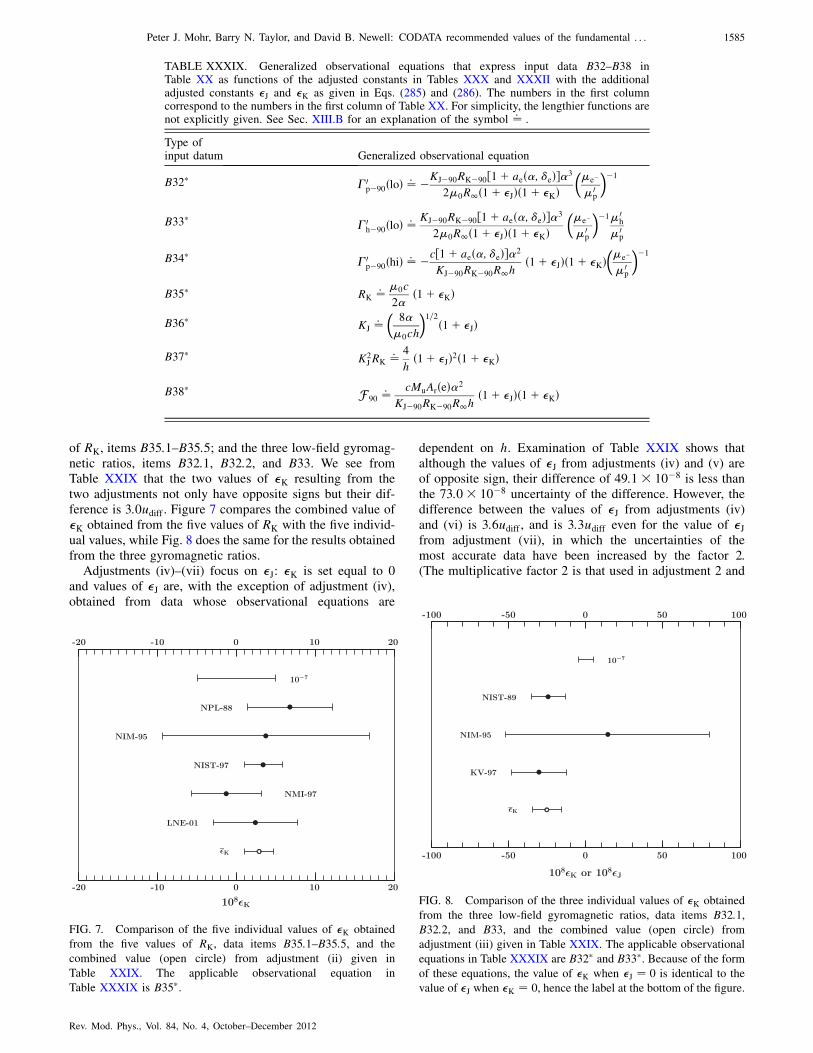
of RK, items B35:1–B35:5; and the three low-field gyromag-netic ratios, items B32:1, B32:2, and B33. We see fromTable XXIX that the two values of �K resulting from thetwo adjustments not only have opposite signs but their dif-ference is 3:0udiff . Figure 7 compares the combined value of�K obtained from the five values of RK with the five individ-ual values, while Fig. 8 does the same for the results obtainedfrom the three gyromagnetic ratios.
Adjustments (iv)–(vii) focus on �J: �K is set equal to 0and values of �J are, with the exception of adjustment (iv),obtained from data whose observational equations are
dependent on h. Examination of Table XXIX shows thatalthough the values of �J from adjustments (iv) and (v) areof opposite sign, their difference of 49:1� 10�8 is less thanthe 73:0� 10�8 uncertainty of the difference. However, thedifference between the values of �J from adjustments (iv)and (vi) is 3:6udiff , and is 3:3udiff even for the value of �Jfrom adjustment (vii), in which the uncertainties of themost accurate data have been increased by the factor 2.(The multiplicative factor 2 is that used in adjustment 2 and
FIG. 7. Comparison of the five individual values of �K obtained
from the five values of RK, data items B35:1–B35:5, and the
combined value (open circle) from adjustment (ii) given in
Table XXIX. The applicable observational equation in
Table XXXIX is B35�.
FIG. 8. Comparison of the three individual values of �K obtained
from the three low-field gyromagnetic ratios, data items B32:1,B32:2, and B33, and the combined value (open circle) from
adjustment (iii) given in Table XXIX. The applicable observational
equations in Table XXXIX are B32� and B33�. Because of the formof these equations, the value of �K when �J ¼ 0 is identical to the
value of �J when �K ¼ 0, hence the label at the bottom of the figure.
TABLE XXXIX. Generalized observational equations that express input data B32–B38 inTable XX as functions of the adjusted constants in Tables XXX and XXXII with the additionaladjusted constants �J and �K as given in Eqs. (285) and (286). The numbers in the first columncorrespond to the numbers in the first column of Table XX. For simplicity, the lengthier functions arenot explicitly given. See Sec. XIII.B for an explanation of the symbol ¼: .
Type ofinput datum Generalized observational equation
B32� �0p�90ðloÞ ¼
: �KJ�90RK�90½1þ aeð�; �eÞ��3
2�0R1ð1þ �JÞð1þ �KÞ��e�
�0p
��1
B33� �0h�90ðloÞ ¼
: KJ�90RK�90½1þ aeð�; �eÞ��3
2�0R1ð1þ �JÞð1þ �KÞ��e�
�0p
��1�0h
�0p
B34� �0p�90ðhiÞ ¼: �c½1þ aeð�; �eÞ��2
KJ�90RK�90R1hð1þ �JÞð1þ �KÞ
��e�
�0p
��1
B35� RK ¼: �0c
2�ð1þ �KÞ
B36� KJ ¼:�
8�
�0ch
�1=2ð1þ �JÞ
B37� K2JRK ¼: 4
hð1þ �JÞ2ð1þ �KÞ
B38� F 90 ¼: cMuArðeÞ�2
KJ�90RK�90R1hð1þ �JÞð1þ �KÞ
Peter J. Mohr, Barry N. Taylor, and David B. Newell: CODATA recommended values of the fundamental . . . 1585
Rev. Mod. Phys., Vol. 84, No. 4, October–December 2012
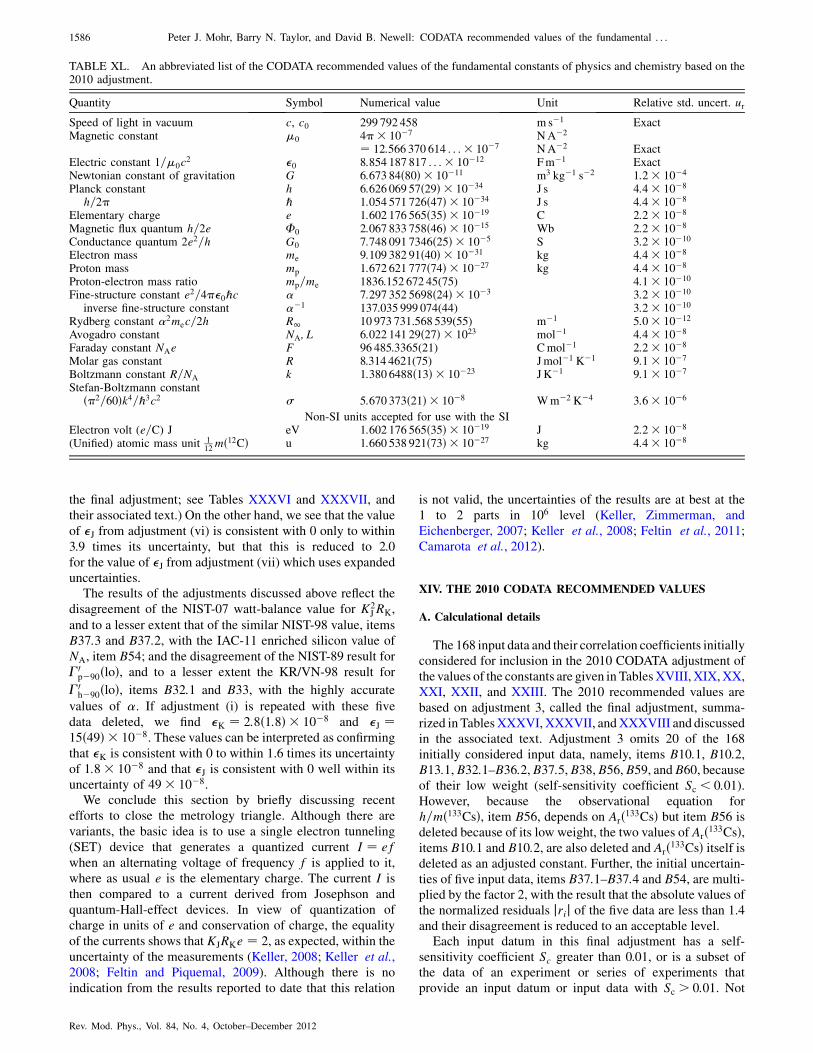
the final adjustment; see Tables XXXVI and XXXVII, and
their associated text.) On the other hand, we see that the value
of �J from adjustment (vi) is consistent with 0 only to within
3.9 times its uncertainty, but that this is reduced to 2.0
for the value of �J from adjustment (vii) which uses expanded
uncertainties.The results of the adjustments discussed above reflect the
disagreement of the NIST-07 watt-balance value for K2JRK,
and to a lesser extent that of the similar NIST-98 value, items
B37:3 and B37:2, with the IAC-11 enriched silicon value of
NA, item B54; and the disagreement of the NIST-89 result for
�0p�90ðloÞ, and to a lesser extent the KR/VN-98 result for
�0h�90ðloÞ, items B32:1 and B33, with the highly accurate
values of �. If adjustment (i) is repeated with these five
data deleted, we find �K ¼ 2:8ð1:8Þ � 10�8 and �J ¼15ð49Þ � 10�8. These values can be interpreted as confirming
that �K is consistent with 0 to within 1.6 times its uncertainty
of 1:8� 10�8 and that �J is consistent with 0 well within its
uncertainty of 49� 10�8.We conclude this section by briefly discussing recent
efforts to close the metrology triangle. Although there are
variants, the basic idea is to use a single electron tunneling
(SET) device that generates a quantized current I ¼ efwhen an alternating voltage of frequency f is applied to it,
where as usual e is the elementary charge. The current I is
then compared to a current derived from Josephson and
quantum-Hall-effect devices. In view of quantization of
charge in units of e and conservation of charge, the equality
of the currents shows that KJRKe ¼ 2, as expected, within theuncertainty of the measurements (Keller, 2008; Keller et al.,
2008; Feltin and Piquemal, 2009). Although there is no
indication from the results reported to date that this relation
is not valid, the uncertainties of the results are at best at the
1 to 2 parts in 106 level (Keller, Zimmerman, and
Eichenberger, 2007; Keller et al., 2008; Feltin et al., 2011;
Camarota et al., 2012).
XIV. THE 2010 CODATA RECOMMENDED VALUES
A. Calculational details
The 168 input data and their correlation coefficients initially
considered for inclusion in the 2010 CODATA adjustment of
the values of the constants are given in Tables XVIII, XIX,XX,
XXI, XXII, and XXIII. The 2010 recommended values are
based on adjustment 3, called the final adjustment, summa-
rized in TablesXXXVI, XXXVII, andXXXVIII and discussed
in the associated text. Adjustment 3 omits 20 of the 168
initially considered input data, namely, items B10:1, B10:2,B13:1,B32:1–B36:2,B37:5,B38,B56,B59, andB60, becauseof their low weight (self-sensitivity coefficient Sc < 0:01).However, because the observational equation for
h=mð133CsÞ, item B56, depends on Arð133CsÞ but item B56 is
deleted because of its low weight, the two values of Arð133CsÞ,items B10:1 and B10:2, are also deleted and Arð133CsÞ itself isdeleted as an adjusted constant. Further, the initial uncertain-
ties of five input data, items B37:1–B37:4 and B54, are multi-
plied by the factor 2, with the result that the absolute values of
the normalized residuals jrij of the five data are less than 1.4
and their disagreement is reduced to an acceptable level.Each input datum in this final adjustment has a self-
sensitivity coefficient Sc greater than 0.01, or is a subset of
the data of an experiment or series of experiments that
provide an input datum or input data with Sc > 0:01. Not
TABLE XL. An abbreviated list of the CODATA recommended values of the fundamental constants of physics and chemistry based on the2010 adjustment.
Quantity Symbol Numerical value Unit Relative std. uncert. ur
Speed of light in vacuum c, c0 299 792 458 ms�1 ExactMagnetic constant �0 4�� 10�7 NA�2
¼ 12:566 370 614 . . .� 10�7 NA�2 ExactElectric constant 1=�0c
2 �0 8:854 187 817 . . .� 10�12 Fm�1 ExactNewtonian constant of gravitation G 6:673 84ð80Þ � 10�11 m3 kg�1 s�2 1:2� 10�4
Planck constant h 6:626 069 57ð29Þ � 10�34 J s 4:4� 10�8
h=2� ℏ 1:054 571 726ð47Þ � 10�34 J s 4:4� 10�8
Elementary charge e 1:602 176 565ð35Þ � 10�19 C 2:2� 10�8
Magnetic flux quantum h=2e �0 2:067 833 758ð46Þ � 10�15 Wb 2:2� 10�8
Conductance quantum 2e2=h G0 7:748 091 7346ð25Þ � 10�5 S 3:2� 10�10
Electron mass me 9:109 382 91ð40Þ � 10�31 kg 4:4� 10�8
Proton mass mp 1:672 621 777ð74Þ � 10�27 kg 4:4� 10�8
Proton-electron mass ratio mp=me 1836.152 672 45(75) 4:1� 10�10
Fine-structure constant e2=4��0ℏc � 7:297 352 5698ð24Þ � 10�3 3:2� 10�10
inverse fine-structure constant ��1 137.035 999 074(44) 3:2� 10�10
Rydberg constant �2mec=2h R1 10 973 731.568 539(55) m�1 5:0� 10�12
Avogadro constant NA; L 6:022 141 29ð27Þ � 1023 mol�1 4:4� 10�8
Faraday constant NAe F 96 485.3365(21) Cmol�1 2:2� 10�8
Molar gas constant R 8.314 4621(75) Jmol�1 K�1 9:1� 10�7
Boltzmann constant R=NA k 1:380 6488ð13Þ � 10�23 J K�1 9:1� 10�7
Stefan-Boltzmann constantð�2=60Þk4=ℏ3c2 � 5:670 373ð21Þ � 10�8 Wm�2 K�4 3:6� 10�6
Non-SI units accepted for use with the SIElectron volt (e=C) J eV 1:602 176 565ð35Þ � 10�19 J 2:2� 10�8
(Unified) atomic mass unit 112mð12CÞ u 1:660 538 921ð73Þ � 10�27 kg 4:4� 10�8
1586 Peter J. Mohr, Barry N. Taylor, and David B. Newell: CODATA recommended values of the fundamental . . .
Rev. Mod. Phys., Vol. 84, No. 4, October–December 2012
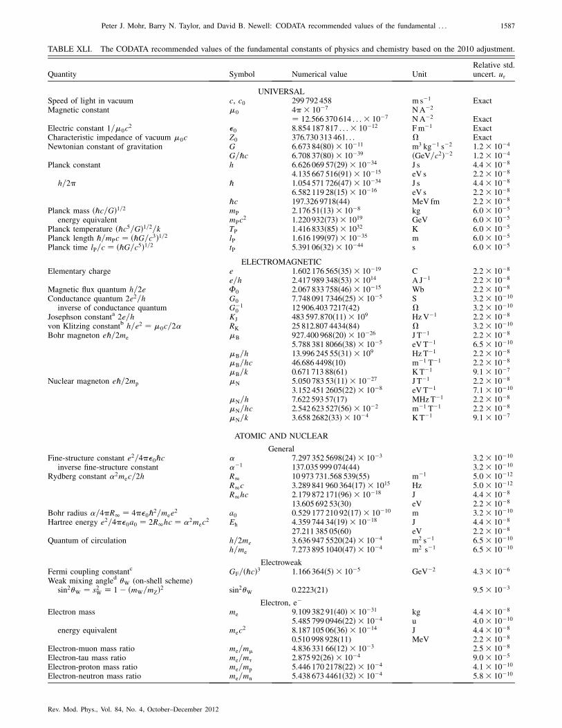
TABLE XLI. The CODATA recommended values of the fundamental constants of physics and chemistry based on the 2010 adjustment.
Quantity Symbol Numerical value UnitRelative std.uncert. ur
UNIVERSALSpeed of light in vacuum c, c0 299 792 458 ms�1 ExactMagnetic constant �0 4�� 10�7 NA�2
¼ 12:566 370 614 . . .� 10�7 NA�2 ExactElectric constant 1=�0c
2 �0 8:854 187 817 . . .� 10�12 Fm�1 ExactCharacteristic impedance of vacuum �0c Z0 376.730 313 461. . . � ExactNewtonian constant of gravitation G 6:673 84ð80Þ � 10�11 m3 kg�1 s�2 1:2� 10�4
G=ℏc 6:708 37ð80Þ � 10�39 ðGeV=c2Þ�2 1:2� 10�4
Planck constant h 6:626 069 57ð29Þ � 10�34 J s 4:4� 10�8
4:135 667 516ð91Þ � 10�15 eV s 2:2� 10�8
h=2� ℏ 1:054 571 726ð47Þ � 10�34 J s 4:4� 10�8
6:582 119 28ð15Þ � 10�16 eV s 2:2� 10�8
ℏc 197.326 9718(44) MeV fm 2:2� 10�8
Planck mass ðℏc=GÞ1=2 mP 2:176 51ð13Þ � 10�8 kg 6:0� 10�5
energy equivalent mPc2 1:220 932ð73Þ � 1019 GeV 6:0� 10�5
Planck temperature ðℏc5=GÞ1=2=k TP 1:416 833ð85Þ � 1032 K 6:0� 10�5
Planck length ℏ=mPc ¼ ðℏG=c3Þ1=2 lP 1:616 199ð97Þ � 10�35 m 6:0� 10�5
Planck time lP=c ¼ ðℏG=c5Þ1=2 tP 5:391 06ð32Þ � 10�44 s 6:0� 10�5
ELECTROMAGNETICElementary charge e 1:602 176 565ð35Þ � 10�19 C 2:2� 10�8
e=h 2:417 989 348ð53Þ � 1014 A J�1 2:2� 10�8
Magnetic flux quantum h=2e �0 2:067 833 758ð46Þ � 10�15 Wb 2:2� 10�8
Conductance quantum 2e2=h G0 7:748 091 7346ð25Þ � 10�5 S 3:2� 10�10
inverse of conductance quantum G�10 12 906.403 7217(42) � 3:2� 10�10
Josephson constanta 2e=h KJ 483 597:870ð11Þ � 109 HzV�1 2:2� 10�8
von Klitzing constantb h=e2 ¼ �0c=2� RK 25 812.807 4434(84) � 3:2� 10�10
Bohr magneton eℏ=2me �B 927:400 968ð20Þ � 10�26 J T�1 2:2� 10�8
5:788 381 8066ð38Þ � 10�5 eVT�1 6:5� 10�10
�B=h 13:996 245 55ð31Þ � 109 Hz T�1 2:2� 10�8
�B=hc 46.686 4498(10) m�1 T�1 2:2� 10�8
�B=k 0.671 713 88(61) KT�1 9:1� 10�7
Nuclear magneton eℏ=2mp �N 5:050 783 53ð11Þ � 10�27 J T�1 2:2� 10�8
3:152 451 2605ð22Þ � 10�8 eVT�1 7:1� 10�10
�N=h 7.622 593 57(17) MHzT�1 2:2� 10�8
�N=hc 2:542 623 527ð56Þ � 10�2 m�1 T�1 2:2� 10�8
�N=k 3:658 2682ð33Þ � 10�4 KT�1 9:1� 10�7
ATOMIC AND NUCLEAR
GeneralFine-structure constant e2=4��0ℏc � 7:297 352 5698ð24Þ � 10�3 3:2� 10�10
inverse fine-structure constant ��1 137.035 999 074(44) 3:2� 10�10
Rydberg constant �2mec=2h R1 10 973 731.568 539(55) m�1 5:0� 10�12
R1c 3:289 841 960 364ð17Þ � 1015 Hz 5:0� 10�12
R1hc 2:179 872 171ð96Þ � 10�18 J 4:4� 10�8
13.605 692 53(30) eV 2:2� 10�8
Bohr radius �=4�R1 ¼ 4��0ℏ2=mee2 a0 0:529 177 210 92ð17Þ � 10�10 m 3:2� 10�10
Hartree energy e2=4��0a0 ¼ 2R1hc ¼ �2mec2 Eh 4:359 744 34ð19Þ � 10�18 J 4:4� 10�8
27.211 385 05(60) eV 2:2� 10�8
Quantum of circulation h=2me 3:636 947 5520ð24Þ � 10�4 m2 s�1 6:5� 10�10
h=me 7:273 895 1040ð47Þ � 10�4 m2 s�1 6:5� 10�10
ElectroweakFermi coupling constantc GF=ðℏcÞ3 1:166 364ð5Þ � 10�5 GeV�2 4:3� 10�6
Weak mixing angled �W (on-shell scheme)sin2�W ¼ s2W � 1� ðmW=mZÞ2 sin2�W 0.2223(21) 9:5� 10�3
Electron, e�Electron mass me 9:109 382 91ð40Þ � 10�31 kg 4:4� 10�8
5:485 799 0946ð22Þ � 10�4 u 4:0� 10�10
energy equivalent mec2 8:187 105 06ð36Þ � 10�14 J 4:4� 10�8
0.510 998 928(11) MeV 2:2� 10�8
Electron-muon mass ratio me=m� 4:836 331 66ð12Þ � 10�3 2:5� 10�8
Electron-tau mass ratio me=m� 2:875 92ð26Þ � 10�4 9:0� 10�5
Electron-proton mass ratio me=mp 5:446 170 2178ð22Þ � 10�4 4:1� 10�10
Electron-neutron mass ratio me=mn 5:438 673 4461ð32Þ � 10�4 5:8� 10�10
Peter J. Mohr, Barry N. Taylor, and David B. Newell: CODATA recommended values of the fundamental . . . 1587
Rev. Mod. Phys., Vol. 84, No. 4, October–December 2012
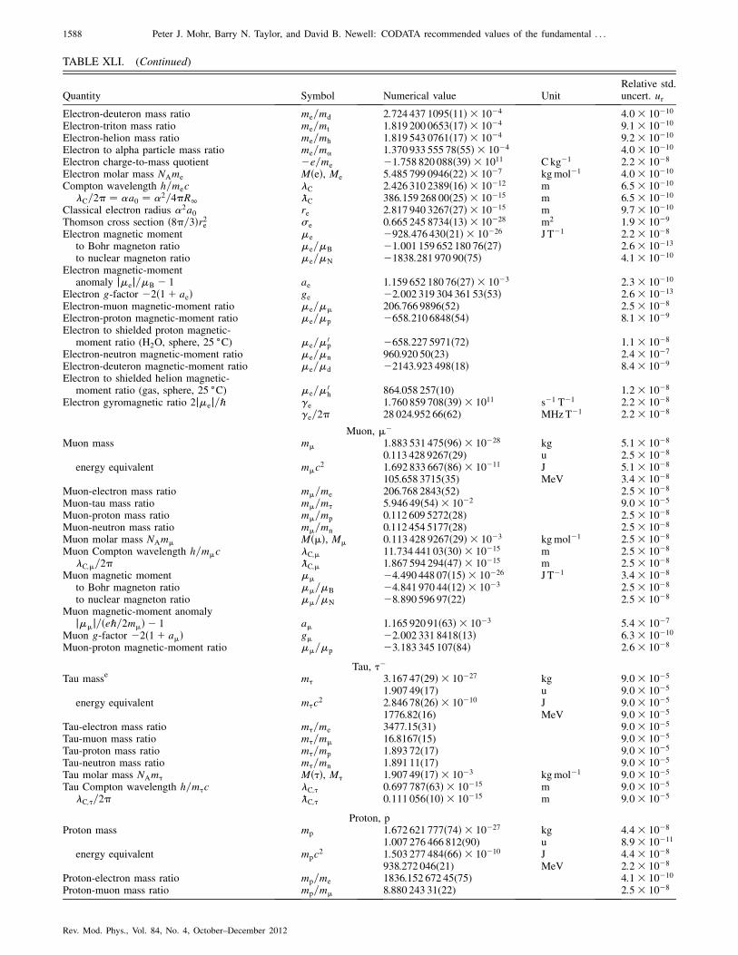
Quantity Symbol Numerical value UnitRelative std.uncert. ur
Electron-deuteron mass ratio me=md 2:724 437 1095ð11Þ � 10�4 4:0� 10�10
Electron-triton mass ratio me=mt 1:819 200 0653ð17Þ � 10�4 9:1� 10�10
Electron-helion mass ratio me=mh 1:819 543 0761ð17Þ � 10�4 9:2� 10�10
Electron to alpha particle mass ratio me=m� 1:370 933 555 78ð55Þ � 10�4 4:0� 10�10
Electron charge-to-mass quotient �e=me �1:758 820 088ð39Þ � 1011 C kg�1 2:2� 10�8
Electron molar mass NAme MðeÞ, Me 5:485 799 0946ð22Þ � 10�7 kgmol�1 4:0� 10�10
Compton wavelength h=mec C 2:426 310 2389ð16Þ � 10�12 m 6:5� 10�10
C=2� ¼ �a0 ¼ �2=4�R1 C 386:159 268 00ð25Þ � 10�15 m 6:5� 10�10
Classical electron radius �2a0 re 2:817 940 3267ð27Þ � 10�15 m 9:7� 10�10
Thomson cross section ð8�=3Þr2e �e 0:665 245 8734ð13Þ � 10�28 m2 1:9� 10�9
Electron magnetic moment �e �928:476 430ð21Þ � 10�26 J T�1 2:2� 10�8
to Bohr magneton ratio �e=�B �1:001 159 652 180 76ð27Þ 2:6� 10�13
to nuclear magneton ratio �e=�N �1838:281 970 90ð75Þ 4:1� 10�10
Electron magnetic-momentanomaly j�ej=�B � 1 ae 1:159 652 180 76ð27Þ � 10�3 2:3� 10�10
Electron g-factor �2ð1þ aeÞ ge �2:002 319 304 361 53ð53Þ 2:6� 10�13
Electron-muon magnetic-moment ratio �e=�� 206.766 9896(52) 2:5� 10�8
Electron-proton magnetic-moment ratio �e=�p �658:210 6848ð54Þ 8:1� 10�9
Electron to shielded proton magnetic-moment ratio (H2O, sphere, 25
�C) �e=�0p �658:227 5971ð72Þ 1:1� 10�8
Electron-neutron magnetic-moment ratio �e=�n 960.920 50(23) 2:4� 10�7
Electron-deuteron magnetic-moment ratio �e=�d �2143:923 498ð18Þ 8:4� 10�9
Electron to shielded helion magnetic-moment ratio (gas, sphere, 25 �C) �e=�
0h 864.058 257(10) 1:2� 10�8
Electron gyromagnetic ratio 2j�ej=ℏ �e 1:760 859 708ð39Þ � 1011 s�1 T�1 2:2� 10�8
�e=2� 28 024.952 66(62) MHzT�1 2:2� 10�8
Muon, ��Muon mass m� 1:883 531 475ð96Þ � 10�28 kg 5:1� 10�8
0.113 428 9267(29) u 2:5� 10�8
energy equivalent m�c2 1:692 833 667ð86Þ � 10�11 J 5:1� 10�8
105.658 3715(35) MeV 3:4� 10�8
Muon-electron mass ratio m�=me 206.768 2843(52) 2:5� 10�8
Muon-tau mass ratio m�=m� 5:946 49ð54Þ � 10�2 9:0� 10�5
Muon-proton mass ratio m�=mp 0.112 609 5272(28) 2:5� 10�8
Muon-neutron mass ratio m�=mn 0.112 454 5177(28) 2:5� 10�8
Muon molar mass NAm� Mð�Þ, M� 0:113 428 9267ð29Þ � 10�3 kgmol�1 2:5� 10�8
Muon Compton wavelength h=m�c C;� 11:734 441 03ð30Þ � 10�15 m 2:5� 10�8
C;�=2� C;� 1:867 594 294ð47Þ � 10�15 m 2:5� 10�8
Muon magnetic moment �� �4:490 448 07ð15Þ � 10�26 J T�1 3:4� 10�8
to Bohr magneton ratio ��=�B �4:841 970 44ð12Þ � 10�3 2:5� 10�8
to nuclear magneton ratio ��=�N �8:890 596 97ð22Þ 2:5� 10�8
Muon magnetic-moment anomalyj��j=ðeℏ=2m�Þ � 1 a� 1:165 920 91ð63Þ � 10�3 5:4� 10�7
Muon g-factor �2ð1þ a�Þ g� �2:002 331 8418ð13Þ 6:3� 10�10
Muon-proton magnetic-moment ratio ��=�p �3:183 345 107ð84Þ 2:6� 10�8
Tau, ��Tau masse m� 3:167 47ð29Þ � 10�27 kg 9:0� 10�5
1.907 49(17) u 9:0� 10�5
energy equivalent m�c2 2:846 78ð26Þ � 10�10 J 9:0� 10�5
1776.82(16) MeV 9:0� 10�5
Tau-electron mass ratio m�=me 3477.15(31) 9:0� 10�5
Tau-muon mass ratio m�=m� 16.8167(15) 9:0� 10�5
Tau-proton mass ratio m�=mp 1.893 72(17) 9:0� 10�5
Tau-neutron mass ratio m�=mn 1.891 11(17) 9:0� 10�5
Tau molar mass NAm� Mð�Þ, M� 1:907 49ð17Þ � 10�3 kgmol�1 9:0� 10�5
Tau Compton wavelength h=m�c C;� 0:697 787ð63Þ � 10�15 m 9:0� 10�5
C;�=2� C;� 0:111 056ð10Þ � 10�15 m 9:0� 10�5
Proton, pProton mass mp 1:672 621 777ð74Þ � 10�27 kg 4:4� 10�8
1.007 276 466 812(90) u 8:9� 10�11
energy equivalent mpc2 1:503 277 484ð66Þ � 10�10 J 4:4� 10�8
938.272 046(21) MeV 2:2� 10�8
Proton-electron mass ratio mp=me 1836.152 672 45(75) 4:1� 10�10
Proton-muon mass ratio mp=m� 8.880 243 31(22) 2:5� 10�8
TABLE XLI. (Continued)
1588 Peter J. Mohr, Barry N. Taylor, and David B. Newell: CODATA recommended values of the fundamental . . .
Rev. Mod. Phys., Vol. 84, No. 4, October–December 2012
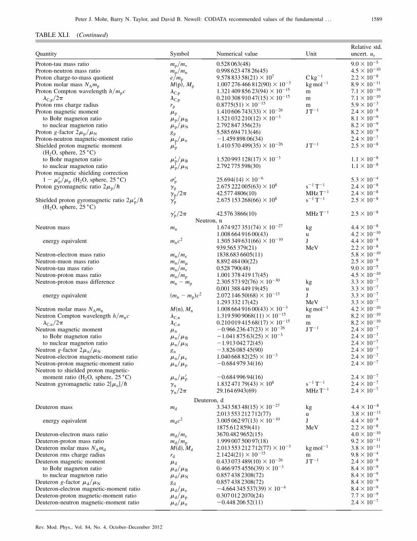
Quantity Symbol Numerical value UnitRelative std.uncert. ur
Proton-tau mass ratio mp=m� 0.528 063(48) 9:0� 10�5
Proton-neutron mass ratio mp=mn 0.998 623 478 26(45) 4:5� 10�10
Proton charge-to-mass quotient e=mp 9:578 833 58ð21Þ � 107 C kg�1 2:2� 10�8
Proton molar mass NAmp MðpÞ, Mp 1:007 276 466 812ð90Þ � 10�3 kgmol�1 8:9� 10�11
Proton Compton wavelength h=mpc C;p 1:321 409 856 23ð94Þ � 10�15 m 7:1� 10�10
C;p=2� C;p 0:210 308 910 47ð15Þ � 10�15 m 7:1� 10�10
Proton rms charge radius rp 0:8775ð51Þ � 10�15 m 5:9� 10�3
Proton magnetic moment �p 1:410 606 743ð33Þ � 10�26 J T�1 2:4� 10�8
to Bohr magneton ratio �p=�B 1:521 032 210ð12Þ � 10�3 8:1� 10�9
to nuclear magneton ratio �p=�N 2.792 847 356(23) 8:2� 10�9
Proton g-factor 2�p=�N gp 5.585 694 713(46) 8:2� 10�9
Proton-neutron magnetic-moment ratio �p=�n �1:459 898 06ð34Þ 2:4� 10�7
Shielded proton magnetic moment �0p 1:410 570 499ð35Þ � 10�26 J T�1 2:5� 10�8
(H2O, sphere, 25�C)
to Bohr magneton ratio �0p=�B 1:520 993 128ð17Þ � 10�3 1:1� 10�8
to nuclear magneton ratio �0p=�N 2.792 775 598(30) 1:1� 10�8
Proton magnetic shielding correction1��0
p=�p (H2O, sphere, 25�C) �0
p 25:694ð14Þ � 10�6 5:3� 10�4
Proton gyromagnetic ratio 2�p=ℏ �p 2:675 222 005ð63Þ � 108 s�1 T�1 2:4� 10�8
�p=2� 42.577 4806(10) MHzT�1 2:4� 10�8
Shielded proton gyromagnetic ratio 2�0p=ℏ
(H2O, sphere, 25�C)
�0p 2:675 153 268ð66Þ � 108 s�1 T�1 2:5� 10�8
�0p=2� 42.576 3866(10) MHzT�1 2:5� 10�8
Neutron, nNeutron mass mn 1:674 927 351ð74Þ � 10�27 kg 4:4� 10�8
1.008 664 916 00(43) u 4:2� 10�10
energy equivalent mnc2 1:505 349 631ð66Þ � 10�10 J 4:4� 10�8
939.565 379(21) MeV 2:2� 10�8
Neutron-electron mass ratio mn=me 1838.683 6605(11) 5:8� 10�10
Neutron-muon mass ratio mn=m� 8.892 484 00(22) 2:5� 10�8
Neutron-tau mass ratio mn=m� 0.528 790(48) 9:0� 10�5
Neutron-proton mass ratio mn=mp 1.001 378 419 17(45) 4:5� 10�10
Neutron-proton mass difference mn �mp 2:305 573 92ð76Þ � 10�30 kg 3:3� 10�7
0.001 388 449 19(45) u 3:3� 10�7
energy equivalent ðmn �mpÞc2 2:072 146 50ð68Þ � 10�13 J 3:3� 10�7
1.293 332 17(42) MeV 3:3� 10�7
Neutron molar mass NAmn MðnÞ;Mn 1:008 664 916 00ð43Þ � 10�3 kgmol�1 4:2� 10�10
Neutron Compton wavelength h=mnc C;n 1:319 590 9068ð11Þ � 10�15 m 8:2� 10�10
C;n=2� C;n 0:210 019 415 68ð17Þ � 10�15 m 8:2� 10�10
Neutron magnetic moment �n �0:966 236 47ð23Þ � 10�26 J T�1 2:4� 10�7
to Bohr magneton ratio �n=�B �1:041 875 63ð25Þ � 10�3 2:4� 10�7
to nuclear magneton ratio �n=�N �1:913 042 72ð45Þ 2:4� 10�7
Neutron g-factor 2�n=�N gn �3:826 085 45ð90Þ 2:4� 10�7
Neutron-electron magnetic-moment ratio �n=�e 1:040 668 82ð25Þ � 10�3 2:4� 10�7
Neutron-proton magnetic-moment ratio �n=�p �0:684 979 34ð16Þ 2:4� 10�7
Neutron to shielded proton magnetic-moment ratio (H2O, sphere, 25
�C) �n=�0p �0:684 996 94ð16Þ 2:4� 10�7
Neutron gyromagnetic ratio 2j�nj=ℏ �n 1:832 471 79ð43Þ � 108 s�1 T�1 2:4� 10�7
�n=2� 29.164 6943(69) MHzT�1 2:4� 10�7
Deuteron, dDeuteron mass md 3:343 583 48ð15Þ � 10�27 kg 4:4� 10�8
2.013 553 212 712(77) u 3:8� 10�11
energy equivalent mdc2 3:005 062 97ð13Þ � 10�10 J 4:4� 10�8
1875.612 859(41) MeV 2:2� 10�8
Deuteron-electron mass ratio md=me 3670.482 9652(15) 4:0� 10�10
Deuteron-proton mass ratio md=mp 1.999 007 500 97(18) 9:2� 10�11
Deuteron molar mass NAmd MðdÞ;Md 2:013 553 212 712ð77Þ � 10�3 kgmol�1 3:8� 10�11
Deuteron rms charge radius rd 2:1424ð21Þ � 10�15 m 9:8� 10�4
Deuteron magnetic moment �d 0:433 073 489ð10Þ � 10�26 J T�1 2:4� 10�8
to Bohr magneton ratio �d=�B 0:466 975 4556ð39Þ � 10�3 8:4� 10�9
to nuclear magneton ratio �d=�N 0.857 438 2308(72) 8:4� 10�9
Deuteron g-factor �d=�N gd 0.857 438 2308(72) 8:4� 10�9
Deuteron-electron magnetic-moment ratio �d=�e �4:664 345 537ð39Þ � 10�4 8:4� 10�9
Deuteron-proton magnetic-moment ratio �d=�p 0.307 012 2070(24) 7:7� 10�9
Deuteron-neutron magnetic-moment ratio �d=�n �0:448 206 52ð11Þ 2:4� 10�7
TABLE XLI. (Continued)
Peter J. Mohr, Barry N. Taylor, and David B. Newell: CODATA recommended values of the fundamental . . . 1589
Rev. Mod. Phys., Vol. 84, No. 4, October–December 2012
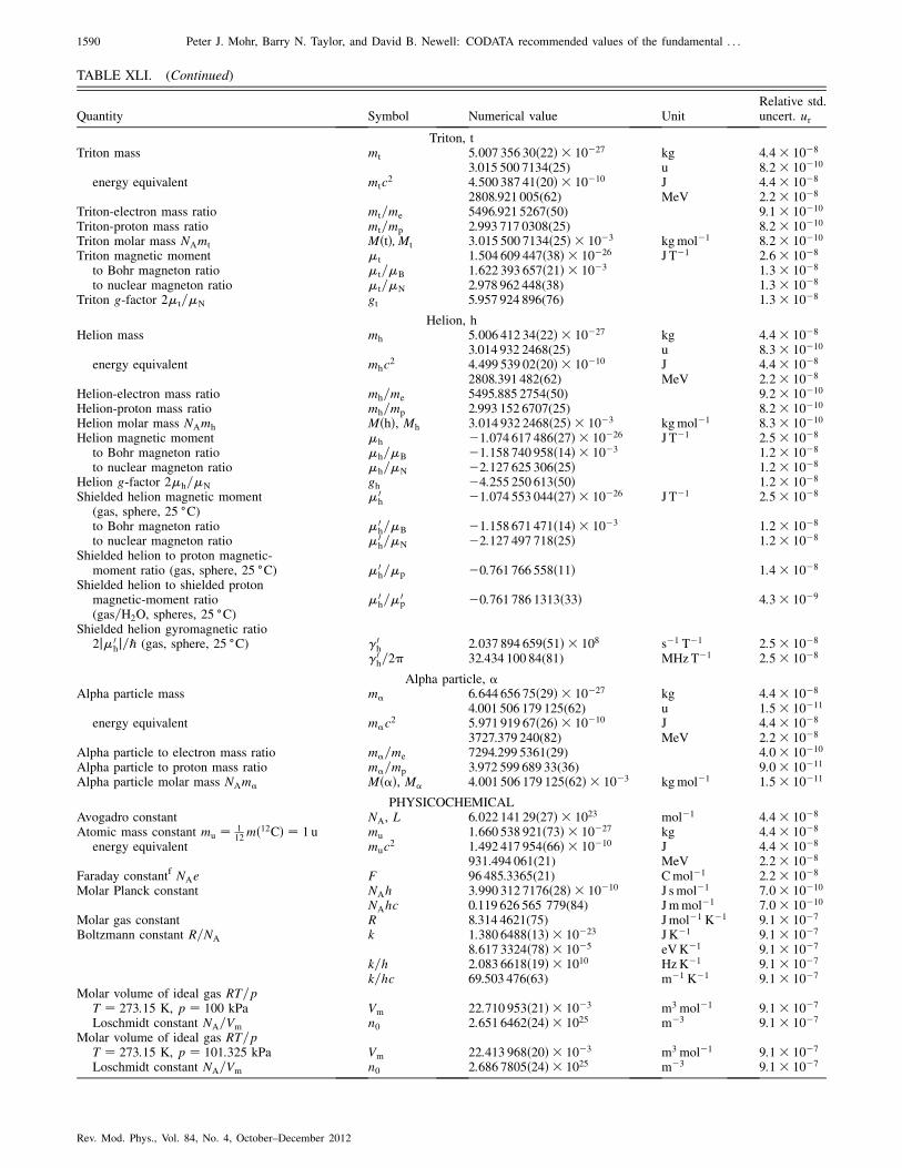
Quantity Symbol Numerical value UnitRelative std.uncert. ur
Triton, tTriton mass mt 5:007 356 30ð22Þ � 10�27 kg 4:4� 10�8
3.015 500 7134(25) u 8:2� 10�10
energy equivalent mtc2 4:500 387 41ð20Þ � 10�10 J 4:4� 10�8
2808.921 005(62) MeV 2:2� 10�8
Triton-electron mass ratio mt=me 5496.921 5267(50) 9:1� 10�10
Triton-proton mass ratio mt=mp 2.993 717 0308(25) 8:2� 10�10
Triton molar mass NAmt MðtÞ;Mt 3:015 500 7134ð25Þ � 10�3 kgmol�1 8:2� 10�10
Triton magnetic moment �t 1:504 609 447ð38Þ � 10�26 J T�1 2:6� 10�8
to Bohr magneton ratio �t=�B 1:622 393 657ð21Þ � 10�3 1:3� 10�8
to nuclear magneton ratio �t=�N 2.978 962 448(38) 1:3� 10�8
Triton g-factor 2�t=�N gt 5.957 924 896(76) 1:3� 10�8
Helion, hHelion mass mh 5:006 412 34ð22Þ � 10�27 kg 4:4� 10�8
3.014 932 2468(25) u 8:3� 10�10
energy equivalent mhc2 4:499 539 02ð20Þ � 10�10 J 4:4� 10�8
2808.391 482(62) MeV 2:2� 10�8
Helion-electron mass ratio mh=me 5495.885 2754(50) 9:2� 10�10
Helion-proton mass ratio mh=mp 2.993 152 6707(25) 8:2� 10�10
Helion molar mass NAmh MðhÞ, Mh 3:014 932 2468ð25Þ � 10�3 kgmol�1 8:3� 10�10
Helion magnetic moment �h �1:074 617 486ð27Þ � 10�26 J T�1 2:5� 10�8
to Bohr magneton ratio �h=�B �1:158 740 958ð14Þ � 10�3 1:2� 10�8
to nuclear magneton ratio �h=�N �2:127 625 306ð25Þ 1:2� 10�8
Helion g-factor 2�h=�N gh �4:255 250 613ð50Þ 1:2� 10�8
Shielded helion magnetic moment(gas, sphere, 25 �C)
�0h �1:074 553 044ð27Þ � 10�26 J T�1 2:5� 10�8
to Bohr magneton ratio �0h=�B �1:158 671 471ð14Þ � 10�3 1:2� 10�8
to nuclear magneton ratio �0h=�N �2:127 497 718ð25Þ 1:2� 10�8
Shielded helion to proton magnetic-moment ratio (gas, sphere, 25 �C) �0
h=�p �0:761 766 558ð11Þ 1:4� 10�8
Shielded helion to shielded protonmagnetic-moment ratio �0
h=�0p �0:761 786 1313ð33Þ 4:3� 10�9
(gas=H2O, spheres, 25�C)
Shielded helion gyromagnetic ratio2j�0
hj=ℏ (gas, sphere, 25 �C) �0h 2:037 894 659ð51Þ � 108 s�1 T�1 2:5� 10�8
�0h=2� 32.434 100 84(81) MHzT�1 2:5� 10�8
Alpha particle, �Alpha particle mass m� 6:644 656 75ð29Þ � 10�27 kg 4:4� 10�8
4.001 506 179 125(62) u 1:5� 10�11
energy equivalent m�c2 5:971 919 67ð26Þ � 10�10 J 4:4� 10�8
3727.379 240(82) MeV 2:2� 10�8
Alpha particle to electron mass ratio m�=me 7294.299 5361(29) 4:0� 10�10
Alpha particle to proton mass ratio m�=mp 3.972 599 689 33(36) 9:0� 10�11
Alpha particle molar mass NAm� Mð�Þ, M� 4:001 506 179 125ð62Þ � 10�3 kgmol�1 1:5� 10�11
PHYSICOCHEMICALAvogadro constant NA, L 6:022 141 29ð27Þ � 1023 mol�1 4:4� 10�8
Atomic mass constant mu ¼ 112mð12CÞ ¼ 1 u mu 1:660 538 921ð73Þ � 10�27 kg 4:4� 10�8
energy equivalent muc2 1:492 417 954ð66Þ � 10�10 J 4:4� 10�8
931.494 061(21) MeV 2:2� 10�8
Faraday constantf NAe F 96 485.3365(21) Cmol�1 2:2� 10�8
Molar Planck constant NAh 3:990 312 7176ð28Þ � 10�10 J smol�1 7:0� 10�10
NAhc 0.119 626 565 779(84) Jmmol�1 7:0� 10�10
Molar gas constant R 8.314 4621(75) Jmol�1 K�1 9:1� 10�7
Boltzmann constant R=NA k 1:380 6488ð13Þ � 10�23 J K�1 9:1� 10�7
8:617 3324ð78Þ � 10�5 eVK�1 9:1� 10�7
k=h 2:083 6618ð19Þ � 1010 HzK�1 9:1� 10�7
k=hc 69.503 476(63) m�1 K�1 9:1� 10�7
Molar volume of ideal gas RT=pT ¼ 273:15 K, p ¼ 100 kPa Vm 22:710 953ð21Þ � 10�3 m3 mol�1 9:1� 10�7
Loschmidt constant NA=Vm n0 2:651 6462ð24Þ � 1025 m�3 9:1� 10�7
Molar volume of ideal gas RT=pT ¼ 273:15 K, p ¼ 101:325 kPa Vm 22:413 968ð20Þ � 10�3 m3 mol�1 9:1� 10�7
Loschmidt constant NA=Vm n0 2:686 7805ð24Þ � 1025 m�3 9:1� 10�7
TABLE XLI. (Continued)
1590 Peter J. Mohr, Barry N. Taylor, and David B. Newell: CODATA recommended values of the fundamental . . .
Rev. Mod. Phys., Vol. 84, No. 4, October–December 2012
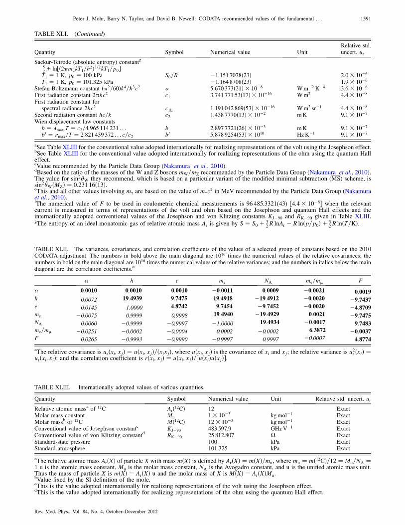
Quantity Symbol Numerical value UnitRelative std.uncert. ur
Sackur-Tetrode (absolute entropy) constantg
52 þ ln½ð2�mukT1=h
2Þ3=2kT1=p0�T1 ¼ 1 K, p0 ¼ 100 kPa S0=R �1:151 7078ð23Þ 2:0� 10�6
T1 ¼ 1 K, p0 ¼ 101:325 kPa �1:164 8708ð23Þ 1:9� 10�6
Stefan-Boltzmann constant ð�2=60Þk4=ℏ3c2 � 5:670 373ð21Þ � 10�8 Wm�2 K�4 3:6� 10�6
First radiation constant 2�hc2 c1 3:741 771 53ð17Þ � 10�16 Wm2 4:4� 10�8
First radiation constant forspectral radiance 2hc2 c1L 1:191 042 869ð53Þ � 10�16 Wm2 sr�1 4:4� 10�8
Second radiation constant hc=k c2 1:438 7770ð13Þ � 10�2 mK 9:1� 10�7
Wien displacement law constantsb ¼ max T ¼ c2=4:965 114 231 . . . b 2:897 7721ð26Þ � 10�3 mK 9:1� 10�7
b0 ¼ �max=T ¼ 2:821 439 372 . . . c=c2 b0 5:878 9254ð53Þ � 1010 HzK�1 9:1� 10�7
aSee Table XLIII for the conventional value adopted internationally for realizing representations of the volt using the Josephson effect.bSee Table XLIII for the conventional value adopted internationally for realizing representations of the ohm using the quantum Halleffect.cValue recommended by the Particle Data Group (Nakamura et al., 2010).dBased on the ratio of the masses of the W and Z bosons mW=mZ recommended by the Particle Data Group (Nakamura et al., 2010).The value for sin2�W they recommend, which is based on a particular variant of the modified minimal subtraction (MS) scheme, issin2�WðMZÞ ¼ 0:231 16ð13Þ.eThis and all other values involving m� are based on the value of m�c
2 in MeV recommended by the Particle Data Group (Nakamuraet al., 2010).fThe numerical value of F to be used in coulometric chemical measurements is 96 485.3321(43) ½4:4� 10�8� when the relevantcurrent is measured in terms of representations of the volt and ohm based on the Josephson and quantum Hall effects and theinternationally adopted conventional values of the Josephson and von Klitzing constants KJ�90 and RK�90 given in Table XLIII.gThe entropy of an ideal monatomic gas of relative atomic mass Ar is given by S ¼ S0 þ 3
2R lnAr � R lnðp=p0Þ þ 52R lnðT=KÞ.
TABLE XLII. The variances, covariances, and correlation coefficients of the values of a selected group of constants based on the 2010CODATA adjustment. The numbers in bold above the main diagonal are 1016 times the numerical values of the relative covariances; thenumbers in bold on the main diagonal are 1016 times the numerical values of the relative variances; and the numbers in italics below the maindiagonal are the correlation coefficients.a
� h e me NA me=m� F
� 0:0010 0:0010 0:0010 �0:0011 0:0009 �0:0021 0:0019h 0.0072 19:4939 9:7475 19:4918 �19:4912 �0:0020 �9:7437e 0.0145 1.0000 4:8742 9:7454 �9:7452 �0:0020 �4:8709me �0.0075 0.9999 0.9998 19:4940 �19:4929 0:0021 �9:7475NA 0.0060 �0.9999 �0.9997 �1.0000 19:4934 �0:0017 9:7483me=m� �0.0251 �0.0002 �0.0004 0.0002 �0.0002 6:3872 �0:0037F 0.0265 �0.9993 �0.9990 �0.9997 0.9997 �0.0007 4:8774
aThe relative covariance is urðxi; xjÞ ¼ uðxi; xjÞ=ðxixjÞ, where uðxi; xjÞ is the covariance of xi and xj; the relative variance is u2r ðxiÞ ¼
urðxi; xiÞ: and the correlation coefficient is rðxi; xjÞ ¼ uðxi; xjÞ=½uðxiÞuðxjÞ�.
TABLE XLIII. Internationally adopted values of various quantities.
Quantity Symbol Numerical value Unit Relative std. uncert. ur
Relative atomic massa of 12C Arð12CÞ 12 ExactMolar mass constant Mu 1� 10�3 kgmol�1 ExactMolar massb of 12C Mð12CÞ 12� 10�3 kgmol�1 ExactConventional value of Josephson constantc KJ�90 483 597.9 GHzV�1 ExactConventional value of von Klitzing constantd RK�90 25 812.807 � ExactStandard-state pressure 100 kPa ExactStandard atmosphere 101.325 kPa Exact
aThe relative atomic mass ArðXÞ of particle X with mass mðXÞ is defined by ArðXÞ ¼ mðXÞ=mu, where mu ¼ mð12CÞ=12 ¼ Mu=NA ¼1 u is the atomic mass constant, Mu is the molar mass constant, NA is the Avogadro constant, and u is the unified atomic mass unit.Thus the mass of particle X is mðXÞ ¼ ArðXÞ u and the molar mass of X is MðXÞ ¼ ArðXÞMu.bValue fixed by the SI definition of the mole.cThis is the value adopted internationally for realizing representations of the volt using the Josephson effect.dThis is the value adopted internationally for realizing representations of the ohm using the quantum Hall effect.
TABLE XLI. (Continued)
Peter J. Mohr, Barry N. Taylor, and David B. Newell: CODATA recommended values of the fundamental . . . 1591
Rev. Mod. Phys., Vol. 84, No. 4, October–December 2012
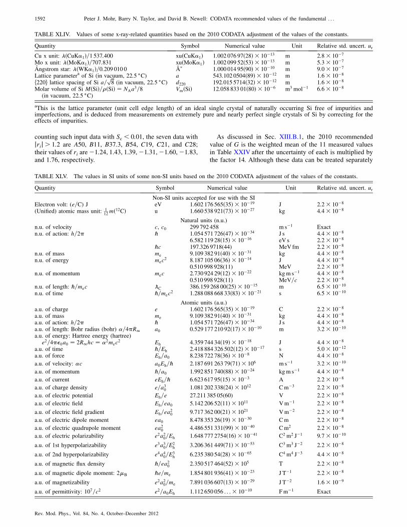
counting such input data with Sc < 0:01, the seven data withjrij> 1:2 are A50, B11, B37:3, B54, C19, C21, and C28;their values of ri are�1:24, 1.43, 1.39,�1:31,�1:60,�1:83,and 1.76, respectively.
As discussed in Sec. XIII.B.1, the 2010 recommendedvalue of G is the weighted mean of the 11 measured valuesin Table XXIV after the uncertainty of each is multiplied bythe factor 14. Although these data can be treated separately
TABLE XLIV. Values of some x-ray-related quantities based on the 2010 CODATA adjustment of the values of the constants.
Quantity Symbol Numerical value Unit Relative std. uncert. ur
Cu x unit: ðCuK�1Þ=1 537:400 xuðCuK�1Þ 1:002 076 97ð28Þ � 10�13 m 2:8� 10�7
Mo x unit: ðMoK�1Þ=707:831 xuðMoK�1Þ 1:002 099 52ð53Þ � 10�13 m 5:3� 10�7
Angstrom star: ðWK�1Þ=0:209 010 0 �A� 1:000 014 95ð90Þ � 10�10 m 9:0� 10�7
Lattice parametera of Si (in vacuum, 22:5 �C) a 543:102 0504ð89Þ � 10�12 m 1:6� 10�8
f220g lattice spacing of Si a=ffiffiffi8
p(in vacuum, 22:5 �C) d220 192:015 5714ð32Þ � 10�12 m 1:6� 10�8
Molar volume of Si MðSiÞ=�ðSiÞ ¼ NAa3=8
(in vacuum, 22:5 �C)VmðSiÞ 12:058 833 01ð80Þ � 10�6 m3 mol�1 6:6� 10�8
aThis is the lattice parameter (unit cell edge length) of an ideal single crystal of naturally occurring Si free of impurities andimperfections, and is deduced from measurements on extremely pure and nearly perfect single crystals of Si by correcting for theeffects of impurities.
TABLE XLV. The values in SI units of some non-SI units based on the 2010 CODATA adjustment of the values of the constants.
Quantity Symbol Numerical value Unit Relative std. uncert. ur
Non-SI units accepted for use with the SIElectron volt: (e=C) J eV 1:602 176 565ð35Þ � 10�19 J 2:2� 10�8
(Unified) atomic mass unit: 112mð12CÞ u 1:660 538 921ð73Þ � 10�27 kg 4:4� 10�8
Natural units (n.u.)n.u. of velocity c, c0 299 792 458 ms�1 Exactn.u. of action: h=2� ℏ 1:054 571 726ð47Þ � 10�34 J s 4:4� 10�8
6:582 119 28ð15Þ � 10�16 eV s 2:2� 10�8
ℏc 197.326 9718(44) MeV fm 2:2� 10�8
n.u. of mass me 9:109 382 91ð40Þ � 10�31 kg 4:4� 10�8
n.u. of energy mec2 8:187 105 06ð36Þ � 10�14 J 4:4� 10�8
0.510 998 928(11) MeV 2:2� 10�8
n.u. of momentum mec 2:730 924 29ð12Þ � 10�22 kgm s�1 4:4� 10�8
0.510 998 928(11) MeV=c 2:2� 10�8
n.u. of length: ℏ=mec C 386:159 268 00ð25Þ � 10�15 m 6:5� 10�10
n.u. of time ℏ=mec2 1:288 088 668 33ð83Þ � 10�21 s 6:5� 10�10
Atomic units (a.u.)a.u. of charge e 1:602 176 565ð35Þ � 10�19 C 2:2� 10�8
a.u. of mass me 9:109 382 91ð40Þ � 10�31 kg 4:4� 10�8
a.u. of action: h=2� ℏ 1:054 571 726ð47Þ � 10�34 J s 4:4� 10�8
a.u. of length: Bohr radius (bohr) �=4�R1 a0 0:529 177 210 92ð17Þ � 10�10 m 3:2� 10�10
a.u. of energy: Hartree energy (hartree)e2=4��0a0 ¼ 2R1hc ¼ �2mec
2 Eh 4:359 744 34ð19Þ � 10�18 J 4:4� 10�8
a.u. of time ℏ=Eh 2:418 884 326 502ð12Þ � 10�17 s 5:0� 10�12
a.u. of force Eh=a0 8:238 722 78ð36Þ � 10�8 N 4:4� 10�8
a.u. of velocity: �c a0Eh=ℏ 2:187 691 263 79ð71Þ � 106 m s�1 3:2� 10�10
a.u. of momentum ℏ=a0 1:992 851 740ð88Þ � 10�24 kgm s�1 4:4� 10�8
a.u. of current eEh=ℏ 6:623 617 95ð15Þ � 10�3 A 2:2� 10�8
a.u. of charge density e=a30 1:081 202 338ð24Þ � 1012 Cm�3 2:2� 10�8
a.u. of electric potential Eh=e 27.211 385 05(60) V 2:2� 10�8
a.u. of electric field Eh=ea0 5:142 206 52ð11Þ � 1011 Vm�1 2:2� 10�8
a.u. of electric field gradient Eh=ea20 9:717 362 00ð21Þ � 1021 Vm�2 2:2� 10�8
a.u. of electric dipole moment ea0 8:478 353 26ð19Þ � 10�30 Cm 2:2� 10�8
a.u. of electric quadrupole moment ea20 4:486 551 331ð99Þ � 10�40 Cm2 2:2� 10�8
a.u. of electric polarizability e2a20=Eh 1:648 777 2754ð16Þ � 10�41 C2 m2 J�1 9:7� 10�10
a.u. of 1st hyperpolarizability e3a30=E2h 3:206 361 449ð71Þ � 10�53 C3 m3 J�2 2:2� 10�8
a.u. of 2nd hyperpolarizability e4a40=E3h 6:235 380 54ð28Þ � 10�65 C4 m4 J�3 4:4� 10�8
a.u. of magnetic flux density ℏ=ea20 2:350 517 464ð52Þ � 105 T 2:2� 10�8
a.u. of magnetic dipole moment: 2�B ℏe=me 1:854 801 936ð41Þ � 10�23 J T�1 2:2� 10�8
a.u. of magnetizability e2a20=me 7:891 036 607ð13Þ � 10�29 J T�2 1:6� 10�9
a.u. of permittivity: 107=c2 e2=a0Eh 1:112 650 056 . . .� 10�10 Fm�1 Exact
1592 Peter J. Mohr, Barry N. Taylor, and David B. Newell: CODATA recommended values of the fundamental . . .
Rev. Mod. Phys., Vol. 84, No. 4, October–December 2012
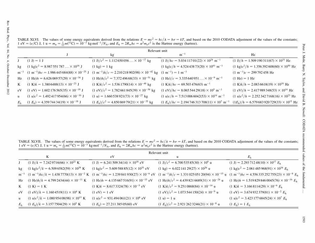
TABLE XLVI. The values of some energy equivalents derived from the relations E ¼ mc2 ¼ hc= ¼ h� ¼ kT, and based on the 2010 CODATA adjustment of the values of the constants;1 eV ¼ ðe=CÞ J, 1 u ¼ mu ¼ 1
12mð12CÞ ¼ 10�3 kgmol�1=NA, and Eh ¼ 2R1hc ¼ �2mec2 is the Hartree energy (hartree).
Relevant unitJ kg m�1 Hz
J ð1 JÞ ¼ 1 J ð1 JÞ=c2 ¼ 1:112 650 056 . . .� 10�17 kg ð1 JÞ=hc ¼ 5:034 117 01ð22Þ � 1024 m�1 ð1 JÞ=h ¼ 1:509 190 311ð67Þ � 1033 Hz
kg ð1 kgÞc2 ¼ 8:987 551 787 . . .� 1016 J ð1 kgÞ ¼ 1 kg ð1 kgÞc=h ¼ 4:524 438 73ð20Þ � 1041 m�1 ð1 kgÞc2=h ¼ 1:356 392 608ð60Þ � 1050 Hz
m�1 ð1 m�1Þhc ¼ 1:986 445 684ð88Þ � 10�25 J ð1 m�1Þh=c ¼ 2:210 218 902ð98Þ � 10�42 kg ð1 m�1Þ ¼ 1 m�1 ð1 m�1Þc ¼ 299 792 458 Hz
Hz ð1 HzÞh ¼ 6:626 069 57ð29Þ � 10�34 J ð1 HzÞh=c2 ¼ 7:372 496 68ð33Þ � 10�51 kg ð1 HzÞ=c ¼ 3:335 640 951 . . .� 10�9 m�1 ð1 HzÞ ¼ 1 Hz
K ð1 KÞk ¼ 1:380 6488ð13Þ � 10�23 J ð1 KÞk=c2 ¼ 1:536 1790ð14Þ � 10�40 kg ð1 KÞk=hc ¼ 69:503 476ð63Þ m�1 ð1 KÞk=h ¼ 2:083 6618ð19Þ � 1010 Hz
eV ð1 eVÞ ¼ 1:602 176 565ð35Þ � 10�19 J ð1 eVÞ=c2 ¼ 1:782 661 845ð39Þ � 10�36 kg ð1 eVÞ=hc ¼ 8:065 544 29ð18Þ � 105 m�1 ð1 eVÞ=h ¼ 2:417 989 348ð53Þ � 1014 Hz
u ð1 uÞc2 ¼ 1:492 417 954ð66Þ � 10�10 J ð1 uÞ ¼ 1:660 538 921ð73Þ � 10�27 kg ð1 uÞc=h ¼ 7:513 006 6042ð53Þ � 1014 m�1 ð1 uÞc2=h ¼ 2:252 342 7168ð16Þ � 1023 Hz
Eh ð1 EhÞ ¼ 4:359 744 34ð19Þ � 10�18 J ð1 EhÞ=c2 ¼ 4:850 869 79ð21Þ � 10�35 kg ð1 EhÞ=hc ¼ 2:194 746 313 708ð11Þ � 107 m�1 ð1EhÞ=h ¼ 6:579 683 920 729ð33Þ � 1015 Hz
TABLE XLVII. The values of some energy equivalents derived from the relations E ¼ mc2 ¼ hc= ¼ h� ¼ kT, and based on the 2010 CODATA adjustment of the values of the constants;1 eV ¼ ðe=CÞ J, 1 u ¼ mu ¼ 1
12mð12CÞ ¼ 10�3 kgmol�1=NA, and Eh ¼ 2R1hc ¼ �2mec2 is the Hartree energy (hartree).
Relevant unitK eV u Eh
J ð1 JÞ=k ¼ 7:242 9716ð66Þ � 1022 K ð1 JÞ ¼ 6:241 509 34ð14Þ � 1018 eV ð1 JÞ=c2 ¼ 6:700 535 85ð30Þ � 109 u ð1 JÞ ¼ 2:293 712 48ð10Þ � 1017 Eh
kg ð1 kgÞc2=k ¼ 6:509 6582ð59Þ � 1039 K ð1 kgÞc2 ¼ 5:609 588 85ð12Þ � 1035 eV ð1 kgÞ ¼ 6:022 141 29ð27Þ � 1026 u ð1 kgÞc2 ¼ 2:061 485 968ð91Þ � 1034 Eh
m�1 ð1 m�1Þhc=k ¼ 1:438 7770ð13Þ � 10�2 K ð1 m�1Þhc ¼ 1:239 841 930ð27Þ � 10�6 eV ð1 m�1Þh=c ¼ 1:331 025 051 20ð94Þ � 10�15 u ð1 m�1Þhc ¼ 4:556 335 252 755ð23Þ � 10�8 Eh
Hz ð1 HzÞh=k ¼ 4:799 2434ð44Þ � 10�11 K ð1 HzÞh ¼ 4:135 667 516ð91Þ � 10�15 eV ð1 HzÞh=c2 ¼ 4:439 821 6689ð31Þ � 10�24 u ð1 HzÞh ¼ 1:519 829 846 0045ð76Þ � 10�16 Eh
K ð1 KÞ ¼ 1 K ð1 KÞk ¼ 8:617 3324ð78Þ � 10�5 eV ð1 KÞk=c2 ¼ 9:251 0868ð84Þ � 10�14 u ð1 KÞk ¼ 3:166 8114ð29Þ � 10�6 Eh
eV ð1 eVÞ=k ¼ 1:160 4519ð11Þ � 104 K ð1 eVÞ ¼ 1 eV ð1 eVÞ=c2 ¼ 1:073 544 150ð24Þ � 10�9 u ð1 eVÞ ¼ 3:674 932 379ð81Þ � 10�2 Eh
u ð1 uÞc2=k ¼ 1:080 954 08ð98Þ � 1013 K ð1 uÞc2 ¼ 931:494 061ð21Þ � 106 eV ð1 uÞ ¼ 1 u ð1 uÞc2 ¼ 3:423 177 6845ð24Þ � 107 Eh
Eh ð1 EhÞ=k ¼ 3:157 7504ð29Þ � 105 K ð1 EhÞ ¼ 27:211 385 05ð60Þ eV ð1 EhÞ=c2 ¼ 2:921 262 3246ð21Þ � 10�8 u ð1 EhÞ ¼ 1 Eh
Peter
J.Mohr,Barry
N.Taylor,andDavid
B.New
ell:CODATA
recommended
valu
esofthefundam
ental
...1593
Rev.
Mod.Phys.,
Vol.84,No.4,Octo
ber–
Decem
ber
2012
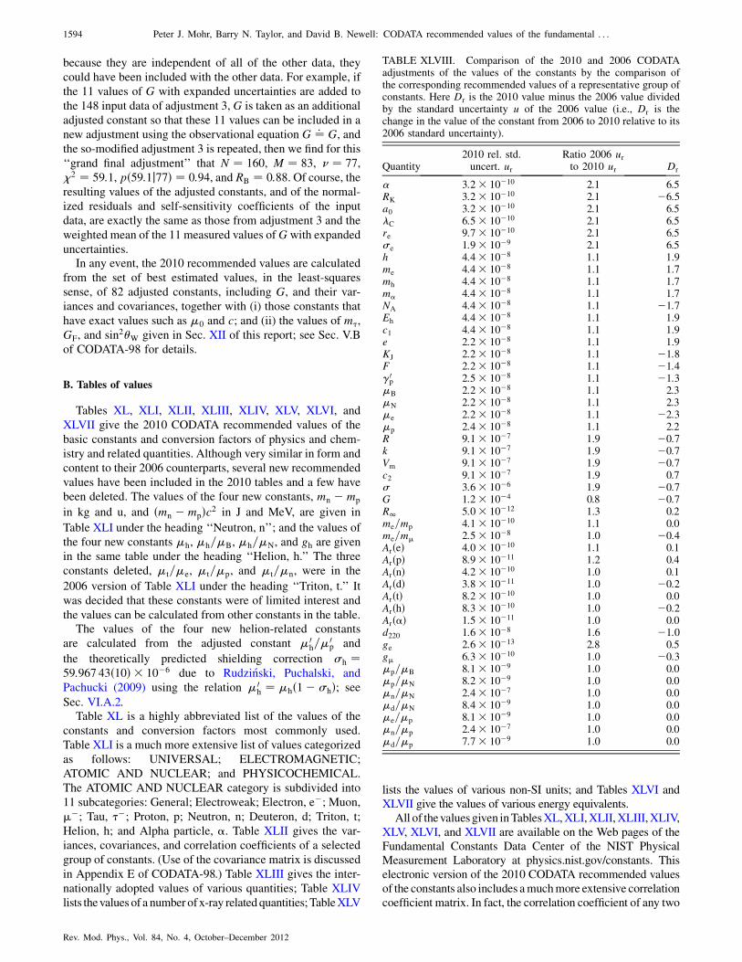
because they are independent of all of the other data, they
could have been included with the other data. For example, if
the 11 values of G with expanded uncertainties are added to
the 148 input data of adjustment 3, G is taken as an additional
adjusted constant so that these 11 values can be included in a
new adjustment using the observational equation G ¼: G, and
the so-modified adjustment 3 is repeated, then we find for this
‘‘grand final adjustment’’ that N ¼ 160, M ¼ 83, � ¼ 77,�2 ¼ 59:1, pð59:1j77Þ ¼ 0:94, and RB ¼ 0:88. Of course, theresulting values of the adjusted constants, and of the normal-
ized residuals and self-sensitivity coefficients of the input
data, are exactly the same as those from adjustment 3 and the
weighted mean of the 11 measured values ofGwith expanded
uncertainties.In any event, the 2010 recommended values are calculated
from the set of best estimated values, in the least-squares
sense, of 82 adjusted constants, including G, and their var-
iances and covariances, together with (i) those constants that
have exact values such as �0 and c; and (ii) the values of m�,
GF, and sin2�W given in Sec. XII of this report; see Sec. V.B
of CODATA-98 for details.
B. Tables of values
Tables XL, XLI, XLII, XLIII, XLIV, XLV, XLVI, and
XLVII give the 2010 CODATA recommended values of the
basic constants and conversion factors of physics and chem-
istry and related quantities. Although very similar in form and
content to their 2006 counterparts, several new recommended
values have been included in the 2010 tables and a few have
been deleted. The values of the four new constants, mn �mp
in kg and u, and ðmn �mpÞc2 in J and MeV, are given in
Table XLI under the heading ‘‘Neutron, n’’; and the values of
the four new constants �h, �h=�B, �h=�N, and gh are givenin the same table under the heading ‘‘Helion, h.’’ The three
constants deleted, �t=�e, �t=�p, and �t=�n, were in the
2006 version of Table XLI under the heading ‘‘Triton, t.’’ It
was decided that these constants were of limited interest and
the values can be calculated from other constants in the table.The values of the four new helion-related constants
are calculated from the adjusted constant �0h=�
0p and
the theoretically predicted shielding correction �h ¼59:967 43ð10Þ � 10�6 due to Rudzinski, Puchalski, and
Pachucki (2009) using the relation �0h ¼ �hð1� �hÞ; see
Sec. VI.A.2.Table XL is a highly abbreviated list of the values of the
constants and conversion factors most commonly used.
Table XLI is a much more extensive list of values categorized
as follows: UNIVERSAL; ELECTROMAGNETIC;
ATOMIC AND NUCLEAR; and PHYSICOCHEMICAL.
The ATOMIC AND NUCLEAR category is subdivided into
11 subcategories: General; Electroweak; Electron, e�; Muon,
��; Tau, ��; Proton, p; Neutron, n; Deuteron, d; Triton, t;Helion, h; and Alpha particle, �. Table XLII gives the var-
iances, covariances, and correlation coefficients of a selected
group of constants. (Use of the covariance matrix is discussed
in Appendix E of CODATA-98.) Table XLIII gives the inter-
nationally adopted values of various quantities; Table XLIV
lists thevalues of a number ofx-ray related quantities;TableXLV
lists the values of various non-SI units; and Tables XLVI andXLVII give the values of various energy equivalents.
All of thevalues given inTablesXL,XLI,XLII,XLIII,XLIV,XLV, XLVI, and XLVII are available on the Web pages of theFundamental Constants Data Center of the NIST PhysicalMeasurement Laboratory at physics.nist.gov/constants. Thiselectronic version of the 2010 CODATA recommended valuesof the constants also includes amuchmore extensive correlationcoefficient matrix. In fact, the correlation coefficient of any two
TABLE XLVIII. Comparison of the 2010 and 2006 CODATAadjustments of the values of the constants by the comparison ofthe corresponding recommended values of a representative group ofconstants. Here Dr is the 2010 value minus the 2006 value dividedby the standard uncertainty u of the 2006 value (i.e., Dr is thechange in the value of the constant from 2006 to 2010 relative to its2006 standard uncertainty).
Quantity2010 rel. std.uncert. ur
Ratio 2006 urto 2010 ur Dr
� 3:2� 10�10 2.1 6.5RK 3:2� 10�10 2.1 �6:5a0 3:2� 10�10 2.1 6.5C 6:5� 10�10 2.1 6.5re 9:7� 10�10 2.1 6.5�e 1:9� 10�9 2.1 6.5h 4:4� 10�8 1.1 1.9me 4:4� 10�8 1.1 1.7mh 4:4� 10�8 1.1 1.7m� 4:4� 10�8 1.1 1.7NA 4:4� 10�8 1.1 �1:7Eh 4:4� 10�8 1.1 1.9c1 4:4� 10�8 1.1 1.9e 2:2� 10�8 1.1 1.9KJ 2:2� 10�8 1.1 �1:8F 2:2� 10�8 1.1 �1:4�0p 2:5� 10�8 1.1 �1:3
�B 2:2� 10�8 1.1 2.3�N 2:2� 10�8 1.1 2.3�e 2:2� 10�8 1.1 �2:3�p 2:4� 10�8 1.1 2.2R 9:1� 10�7 1.9 �0:7k 9:1� 10�7 1.9 �0:7Vm 9:1� 10�7 1.9 �0:7c2 9:1� 10�7 1.9 0.7� 3:6� 10�6 1.9 �0:7G 1:2� 10�4 0.8 �0:7R1 5:0� 10�12 1.3 0.2me=mp 4:1� 10�10 1.1 0.0me=m� 2:5� 10�8 1.0 �0:4ArðeÞ 4:0� 10�10 1.1 0.1ArðpÞ 8:9� 10�11 1.2 0.4ArðnÞ 4:2� 10�10 1.0 0.1ArðdÞ 3:8� 10�11 1.0 �0:2ArðtÞ 8:2� 10�10 1.0 0.0ArðhÞ 8:3� 10�10 1.0 �0:2Arð�Þ 1:5� 10�11 1.0 0.0d220 1:6� 10�8 1.6 �1:0ge 2:6� 10�13 2.8 0.5g� 6:3� 10�10 1.0 �0:3�p=�B 8:1� 10�9 1.0 0.0�p=�N 8:2� 10�9 1.0 0.0�n=�N 2:4� 10�7 1.0 0.0�d=�N 8:4� 10�9 1.0 0.0�e=�p 8:1� 10�9 1.0 0.0�n=�p 2:4� 10�7 1.0 0.0�d=�p 7:7� 10�9 1.0 0.0
1594 Peter J. Mohr, Barry N. Taylor, and David B. Newell: CODATA recommended values of the fundamental . . .
Rev. Mod. Phys., Vol. 84, No. 4, October–December 2012
constants listed in the tables is accessible on theWebsite, aswellas the automatic conversion of the value of an energy-relatedquantity expressed in one unit to the corresponding value ex-pressed in another unit (in essence, an automated version ofTables XLVI and XLVII).
XV. SUMMARY AND CONCLUSION
The focus of this section is (i) comparison of the 2010 and2006 recommended values of the constants and identificationof those new results that have contributed most to the changesin the 2006 values; (ii) presentation of several conclusionsthat can be drawn from the 2010 recommended values and theinput data on which they are based; and (iii) identification ofnew experimental and theoretical work that can advance ourknowledge of the values of the constants.
Topic (iii) is of special importance in light of the adoption bythe 24thGeneral Conference onWeights andMeasures (CGPM)at its meeting in Paris in October 2011 of Resolution 1 entitled‘‘On the possible future revision of the International System ofUnits, the SI,’’ available on theBIPMWeb site at bipm.org/utils/common/pdf/24_CGPM_Resolutions.pdf.
In brief, this resolution notes the intention of the CIPM topropose, possibly to the 25th CGPM in 2014, a revision of theSI. The ‘‘new SI,’’ as it is called to distinguish it from thecurrent SI, will be the system of units in which seven refer-ence constants, including the Planck constant h, elementarycharge e, Boltzmann constant k, and Avogadro constant NA,have exact assigned values. Resolution 1 also looks toCODATA to provide the necessary values of these four con-stants for the new definition. Details of the proposed new SImay be found in Mills et al. (2011) and the references citedtherein; see also Mohr and Newell (2010) and Taylor (2011).
A. Comparison of 2010 and 2006 CODATA recommended values
Table XLVIII compares the 2010 and 2006 recommendedvalues of a representative group of constants. The fact that thevalues of many constants are obtained from expressions propor-tional to the fine-structure constant �, Planck constant h, ormolar gas constant R raised to various powers leads to theregularities observed in the numbers in columns 2 to 4. Forexample, the first six quantities are obtained from expressionsproportional to �a, where jaj ¼ 1, 2, 3, or 6. The next 15quantities, h through the magnetic moment of the proton �p,
are calculated from expressions containing the factor ha, wherejaj ¼ 1 or 1=2. And the five quantities R through the Stefan-Boltzmannconstant� are proportional toRa,where jaj ¼ 1 or4.
Further comments on some of the entries in Table XLVIIIare as follows.
(i) The large shift in the 2006 recommended value of � ismainly due to the discovery and correction of an error in the
numerically calculated value of the eighth-order coefficientAð8Þ1
in the theoretical expression for ae; see Sec. V.A.1. Its reductionin uncertainty is due to two new results. The first is the 2008improved value of ae obtained at Harvard University with arelative standard uncertainty of 2:4� 10�10 compared to the6:6� 10�10 uncertainty of the earlier Harvard result used inthe 2006 adjustment. The second result is the 2011 improvedLKB atom-recoil value of h=mð87RbÞ with an uncertainty of
1:2� 10�9 compared to the 1:3� 10�8 uncertainty of theearlier LKB result used in 2006. The much reduced uncertainty
of ge is also due to the improved value of �.(ii) The change in the 2006 recommended value of h is due
to the 2011 IAC result for NA with a relative standard uncer-tainty of 3:0� 10�8 obtained using 28Si enriched single crys-
tals. It provides a value of hwith the same uncertainty, which issmaller than the 3:6� 10�8 uncertainty of the value of h from
the 2007 NIST watt-balance measurement of K2JRK; the latter
played the dominant role in determining the 2006 recom-mended value. The two differ by about 18 parts in 108,resulting in a shift of the 2006 recommended value by nearly
twice its uncertainty. In the 2006 adjustment inconsistenciesamong some of the electrical and silicon crystal data (all
involving natural silicon) led the Task Group to increase theuncertainties of these data by the multiplicative factor 1.5 toreduce the inconsistencies to an acceptable level. In the
2010 adjustment, inconsistencies among the data that deter-mine h are reduced to an acceptable level by using a multi-
plicative factor of 2. Consequently the uncertainties of the 2006and 2010 recommended values of h do not differ significantly.
(iii) The 2006 recommended value of the molar gas con-stant R was determined by the 1988 NIST speed-of-sound
result with a relative standard uncertainty of 1:8� 10�6, andto a much lesser extent the 1979 NPL speed-of-sound resultwith an uncertainty of 8:4� 10�6 obtained with a rather
different type of apparatus. The six new data of potentialinterest related to R that became available during the
four years between the 2006 and 2010 adjustments haveuncertainties ranging from 1:2� 10�6 to 12� 10�6 andagree with each other as well as with the NIST and NPL
values. Further, the self-sensitivity coefficients of four of thesix were sufficiently large for them to be included in the 2010
final adjustment, and they are responsible for the small shiftin the 2006 recommended value and the reduction of itsuncertainty by nearly a factor of 2.
(iv) Other constants in Table XLVIII whose changes are
worth noting are the Rydberg constant R1, proton relativeatomic mass ArðpÞ, and f220g natural Si lattice spacing d220.The reduction in uncertainty of R1 is due to improvements in
the theory of H and D energy levels and the 2010 LKB resultfor the 1S1=2–3S1=2 transition frequency in hydrogen with a
relative standard uncertainty of 4:4� 10�12. For ArðpÞ, thereduction in uncertainty is due to the 2008 StockholmUniversity (SMILETRAP) result for the ratio of the cyclotron
frequency of the excited hydrogen molecular ion to that ofthe deuteron, fcðHþ�
2 Þ=fcðdÞ, with a relative uncertainty of
1:7� 10�10. The changes in d220 arise from the omission of
the 1999 PTB result for h=mnd220ðW04Þ, the 2004 NMIJresult for d220ðNR3Þ, the 2007 INRIM results ford220ðW4:2aÞ, and d220ðMO�Þ, and the inclusion of the new
2008 INRIM result for d220ðMO�Þ as well as the new 2009INRIM results for d220ðW04Þ and d220ðW4:2aÞ.
B. Some implications of the 2010 CODATA recommended values
and adjustment for metrology and physics
Conventional electric units. The adoption of the conventional
valuesKJ�90 ¼ 483 597:9 GHz=V andRK�90 ¼ 25 812:807 �for the Josephson and von Klitzing constants in 1990 can be
Peter J. Mohr, Barry N. Taylor, and David B. Newell: CODATA recommended values of the fundamental . . . 1595
Rev. Mod. Phys., Vol. 84, No. 4, October–December 2012
viewed as establishing conventional, practical units of voltageand resistance,V90 and�90, given byV90 ¼ ðKJ�90=KJÞ V and�90 ¼ ðRK=RK�90Þ �. Other conventional electric units fol-low from V90 and �90, for example, A90 ¼ V90=�90, C90 ¼A90 s, W90 ¼ A90V90, F90 ¼ C90=V90, and H90 ¼ �90 s,which are the conventional, practical units of current, charge,power, capacitance, and inductance, respectively (Taylor andMohr, 2001). For the relations between KJ and KJ�90, and RK
and RK�90, the 2010 adjustment gives
KJ ¼ KJ�90½1� 6:3ð2:2Þ � 10�8�; (287)
RK ¼ RK�90½1þ 1:718ð32Þ � 10�8�; (288)
which lead to
V90 ¼ ½1þ 6:3ð2:2Þ � 10�8� V; (289)
�90 ¼ ½1þ 1:718ð32Þ � 10�8� �; (290)
A90 ¼ ½1þ 4:6ð2:2Þ � 10�8� A; (291)
C90 ¼ ½1þ 4:6ð2:2Þ � 10�8� C; (292)
W90 ¼ ½1þ 10:8ð4:4Þ � 10�8� W; (293)
F90 ¼ ½1� 1:718ð32Þ � 10�8� F; (294)
H90 ¼ ½1þ 1:718ð32Þ � 10�8� H: (295)
Equations (289) and (290) show that V90 exceeds V and�90 exceeds � by the fractional amounts 6:3ð2:2Þ � 10�8
and 1:718ð32Þ � 10�8, respectively. Thismeans thatmeasuredvoltages and resistances traceable to the Josephson effect andKJ�90 and the quantumHall effect andRK�90, respectively, aretoo small relative to the SI by these same fractional amounts.However, these differences are well within the 40� 10�8
uncertainty assigned to V90=V and the 10� 10�8 uncertaintyassigned to �90=� by the Consultative Committee forElectricity and Magnetism (CCEM) of the CIPM (Quinn,1989, 2001).
Josephson and quantum Hall effects. Although there isextensive theoretical and experimental evidence for the exact-ness of the Josephson and quantum-Hall-effect relations KJ ¼2e=h and RK ¼ h=e2, and some of the input data available forthe 2010 adjustment provide additional supportive evidencefor these expressions, some other data are not supportive.This dichotomy reflects the rather significant inconsistenciesamong a few key data, particularly the highly accurate IACenriched silicon XRCD result for NA, and the comparablyaccurate NISTwatt-balance result for K2
JRK, and will only be
fully resolved when the inconsistencies are reconciled.The new SI. Implementation of the new SI requires that the
four reference constants h, e, k, and NA must be known withsufficiently small uncertainties to meet current and futuremeasurement needs. However, of equal if not greater impor-tance, the causes of any inconsistencies among the data thatprovide their valuesmust be understood.Although the key datathat provide the 2010 recommended value of kwould appear tobe close tomeeting both requirements, this is not the case for h,e, and NA, which are in fact interrelated. We have
NAh ¼ cArðeÞMu�2
2R1; (296)
e ¼�2�h
�0c
�1=2
: (297)
Since the combined relative standard uncertainty of the2010 recommended values of the constants on the right-handside of Eq. (296) is only 7:0� 10�10, a measurement of hwith a given relative uncertainty, even as small as 5� 10�9,determines NA with essentially the same relative uncertainty.Further, since the recommended value of � has a relativeuncertainty of only 3:2� 10�10, based on Eq. (297) therelative uncertainty of e will be half that of h or NA. Forthese reasons, the 2010 recommended values of h and NA
have the same 4:4� 10�8 relative uncertainty, and the un-certainty of the recommended value of e is 2:2� 10�8.However, these uncertainties are twice as large as they wouldhave been if there were no disagreement between the watt-balance values of h and the enriched silicon XRCD value ofNA. This disagreement led to an increase in the uncertaintiesof the relevant data by a factor of 2. More specifically, ifthe data had been consistent the uncertainties of therecommended values of h and NA would be 2:2� 10�8 and1:1� 10�8 for e. Because these should be sufficiently smallfor the new SI to be implemented, the significance of thedisagreement and the importance of measurements of h andNA are apparent.
Proton radius. The proton rms charge radius rp determined
from the Lamb shift in muonic hydrogen disagrees signifi-cantly with values determined from H and D transitionfrequencies as well as from electron-proton scattering experi-ments. Although the uncertainty of the muonic hydrogenvalue is significantly smaller than the uncertainties of theseother values, its negative impact on the internal consistency ofthe theoretically predicted and experimentally measured fre-quencies, as well as on the value of the Rydberg constant, wasdeemed so severe that the only recourse was not to include itin the final least-squares adjustment on which the 2010recommended values are based.
Muon magnetic-moment anomaly. Despite extensive newtheoretical work, the long-standing significant difference be-tween the theoretically predicted, standard-model value of a�and the experimentally determined value remains unresolved.Because the difference is from 3.3 to possibly 4.5 times thestandard uncertainty of the difference, depending on the waythe all-important hadronic contribution to the theoreticalexpression for a� is evaluated, the theory was not incorpo-
rated in the 2010 adjustment. The recommended values of a�and those of other constants that depend on it are, therefore,based on experiment.
Electron magnetic-moment anomaly, fine-structure con-stant, and QED. The most accurate value of the fine-structureconstant � currently available from a single experiment has arelative standard uncertainty of 3:7� 10�10; it is obtained byequating the QED theoretical expression for the electronmagnetic-moment anomaly ae and the most accurate experi-mental value of ae, obtained from measurements on a singleelectron in a Penning trap. This value of � is in excellentagreement with a competitive experimental value with an
1596 Peter J. Mohr, Barry N. Taylor, and David B. Newell: CODATA recommended values of the fundamental . . .
Rev. Mod. Phys., Vol. 84, No. 4, October–December 2012
uncertainty of 6:6� 10�10. Because the latter is obtained fromthe atom-recoil determination of the quotient h=mð87RbÞ usingatom-interferometry and is only weakly dependent on QEDtheory, the agreement provides one of the most significantconfirmations of quantum electrodynamics.
Newtonian constant of gravitation. The situation regardingmeasurements of G continues to be problematic and hasbecome more so in the past four years. Two new resultswith comparatively small uncertainties have become avail-able for the 2010 adjustment, leading to an increase in thescatter among the now 11 values of G. This has resulted in a20% increase in the uncertainty of the 2010 recommendedvalue compared to that of its 2006 predecessor. Clearly, thereis a continuing problem for the determination of this impor-tant, but poorly known, fundamental constant; the uncertaintyof the 2010 recommended value is now 120 parts in 106.
C. Suggestions for future work
For evaluation of the fundamental constants, it is desirablenot only to have multiple results with competitive uncertain-ties for a given quantity, but also to have one or more resultsobtained by a different method. If the term ‘‘redundant’’ isused to describe such an ideal set of data, there is usually onlylimited redundancy among the key data available for anygiven CODATA adjustment.
With this in mind, based on the preceding discussion, oursuggestions are as follows:
(i) Resolution of the disagreement between the most ac-curate watt-balance result for K2
JRK and the XRCD
result for NA. Approaches to solving this problemmight include new measurements of K2
JRK using watt
balances of different design (or their equivalent) withuncertainties at the 2 to 3 parts in 108 level, a thoroughreview by the researchers involved of their existingmeasurements of this quantity, tests of the exactnessof the relations KJ ¼ 2e=h and RK ¼ h=e2, indepen-dent measurements of the isotopic composition of theenriched silicon crystals and their d220 lattice spacingused in the determination of NA (these are the twoprincipal quantities for which only one measurementexists), and a thorough review by the researchers in-volved of the many corrections required to obtain NA
from the principal quantities measured.(ii) Measurements of k (and related quantities such as k=h)
with uncertainties at the 1 to 3 parts in 106 level usingthe techniques of dielectric gas thermometry, refrac-tive index gas thermometry, noise thermometry, andDoppler broadening. These methods are very differentfrom acoustic gas thermometry, which is the dominantmethod used to date.
(iii) Resolution of the discrepancy between the muonichydrogen inferred value of rp and the spectroscopic
value from H and D transition frequencies. Workunderway on frequency measurements in hydrogenas well as the analysis of ��p and ��d data andpossible measurements in ��h and ��� should pro-vide additional useful information. Independentevaluations of electron-scattering data to determinerp are encouraged as well as verification of the theory
of H, D, and muonic hydrogenlike energy levels.
(iv) Independent calculation of the eighth- and tenth-ordercoefficients in the QED expression for ae, in order toincrease confidence in the value of � from ae.
(v) Resolution of the disagreement between the theoreticalexpression for a� and its experimental value. This
discrepancy along with the discrepancy between the-ory and experiment in muonic hydrogen are two im-portant problems in muon-related physics.
(vi) Determinations of G with an uncertainty of 1 part in105 using new and innovative approaches that mightresolve the disagreements among the measurementsmade within the past three decades.
LIST OF SYMBOLS AND ABBREVIATIONS
AMDC Atomic Mass Data Center, Centre deSpectrometrie Nucleaire et de Spectrometriede Masse, Orsay, France
ArðXÞ Relative atomic mass of X: ArðXÞ ¼mðXÞ=mu
A90 Conventional unit of electric current:A90 ¼ V90=�90
�A� Angstrom star: ðWK�1Þ¼0:209 010 0 �A�ae Electron magnetic-moment anomaly: ae ¼
ðjgej � 2Þ=2a� Muon magnetic-moment anomaly: a� ¼
ðjg�j � 2Þ=2BIPM International Bureau of Weights and
Measures, Sevres, FranceBNL Brookhaven National Laboratory, Upton,
New York, USACERN European Organization for Nuclear
Research, Geneva, SwitzerlandCIPM International Committee for Weights and
MeasuresCODATA Committee on Data for Science and
Technology of the International Councilfor Science
CPT Combined charge conjugation, parity inver-sion, and time reversal
c Speed of light in vacuumd Deuteron (nucleus of deuterium D,
or 2H)d220 f220g lattice spacing of an ideal crystal of
naturally occurring silicon
d220ðXÞ f220g lattice spacing of crystal X of natu-rally occurring silicon
Eb Binding energy
e Symbol for either member of the electron-positron pair; when necessary, e� or eþ isused to indicate the electron or positron
e Elementary charge: absolute value of thecharge of the electron
F Faraday constant: F ¼ NAeFSU Florida State University, Tallahassee,
Florida, USA
FSUJ Friedrich-Schiller University, Jena,Germany
Peter J. Mohr, Barry N. Taylor, and David B. Newell: CODATA recommended values of the fundamental . . . 1597
Rev. Mod. Phys., Vol. 84, No. 4, October–December 2012
F 90 F 90 ¼ ðF=A90Þ AG Newtonian constant of gravitation
g Local acceleration of free fall
gd Deuteron g-factor: gd ¼ �d=�N
ge Electron g-factor: ge ¼ 2�e=�B
gp Proton g-factor: gp ¼ 2�p=�N
g0p Shielded proton g-factor: g0p ¼ 2�0p=�N
gt Triton g-factor: gt ¼ 2�t=�N
gXðYÞ g-factor of particle X in the ground (1S)state of hydrogenic atom Y
g� Muon g-factor: g� ¼ 2��=ðeℏ=2m�ÞGSI Gesellschaft fur Schweironenforschung,
Darmstadt, GermanyHD HD molecule (bound state of hydrogen and
deuterium atoms)HT HT molecule (bound state of hydrogen and
tritium atoms)h Helion (nucleus of 3He)h Planck constant; ℏ ¼ h=2�HarvU Harvard University, Cambridge,
Massachusetts, USAIAC International Avogadro CoordinationILL Institut Max von Laue-Paul Langevin,
Grenoble, FranceINRIM Istituto Nazionale di Ricerca Metrologica,
Torino, ItalyIRMM Institute for Reference Materials and
Measurements, Geel, BelgiumJILA Joint Institute of University of Colorado
and NIST, Boulder, Colorado, USAJINR Joint Institute for Nuclear Research,
Dubna, Russian FederationKRISS Korea Research Institute of Standards and
Science, Taedok Science Town, Republicof Korea
KR/VN KRISS-VNIIM collaborationKJ Josephson constant: KJ ¼ 2e=hKJ�90 Conventional value of the Josephson con-
stant KJ: KJ�90 ¼ 483 597:9 GHzV�1
k Boltzmann constant: k ¼ R=NA
LAMPF Clinton P. AndersonMeson Physics Facilityat Los Alamos National Laboratory, LosAlamos, New Mexico, USA
LKB Laboratoire Kastler-Brossel, Paris, FranceLK/SY LKB and SYRTE collaborationLNE Laboratoire national de metrologie et
d’essais, Trappes, FranceMETAS Federal Office of Metrology, Bern-Wabern,
SwitzerlandMIT Massachusetts Institute of Technology,
Cambridge, Massachusetts, USAMPQ Max-Planck-Institut fur Quantenoptik,
Garching, GermanyMðXÞ Molar mass of X: MðXÞ ¼ ArðXÞMu
Mu Muonium (�þe� atom)Mu Molar mass constant: Mu¼10�3 kgmol�1
mu Unified atomic mass constant: mu ¼mð12CÞ=12
mX, mðXÞ Mass of X (for the electron e, proton p, andother elementary particles, the first symbolis used, i.e., me, mp, etc.)
NA Avogadro constantNIM National Institute of Metrology, Beijing,
People’s Republic of ChinaNIST National Institute of Standards and
Technology, Gaithersburg, Maryland andBoulder, Colorado, USA
NMI National Metrology Institute, Lindfield,Australia
NMIJ National Metrology Institute of Japan,Tsukuba, Japan
NPL National Physical Laboratory, Teddington,UK
n NeutronPTB Physikalisch-Technische Bundesanstalt,
Braunschweig and Berlin, Germanyp Proton�pAHeþ Antiprotonic helium (AHeþ þ �p atom,
A ¼ 3 or 4)QED Quantum electrodynamicspð�2j�Þ Probability that an observed value of chi
square for � degrees of freedom wouldexceed �2
R Molar gas constant�R Ratio of muon anomaly difference fre-
quency to free proton NMR frequencyRB Birge ratio: RB ¼ ð�2=�Þ1=2rd Bound-state rms charge radius of the
deuteronRK von Klitzing constant: RK ¼ h=e2
RK�90 Conventional value of the von Klitzing con-stant RK: RK�90 ¼ 25 812:807 �
rp Bound-state rms charge radius of the protonR1 Rydberg constant: R1 ¼ mec�
2=2hrðxi; xjÞ Correlation coefficient of estimated values
xi and xj: rðxi; xjÞ ¼ uðxi; xjÞ=½uðxiÞuðxjÞ�Sc Self-sensitivity coefficientSI Systeme international d’unites (Inter-
national System of Units)StanfU Stanford University, Stanford, California,
USASU Stockholm University, Stockholm, SwedenStPtrsb St. Petersburg, Russian FederationSYRTE Systemes de reference Temps Espace,
Paris, FranceT Thermodynamic temperatureType A Uncertainty evaluation by the statistical
analysis of series of observationsType B Uncertainty evaluation by means other than
the statistical analysis of series of observationst90 Celsius temperature on the International
Temperature Scale of 1990 (ITS-90)t Triton (nucleus of tritium T, or 3H)USus University of Sussex, Sussex, UKUWash University of Washington, Seattle,
Washington, USA
1598 Peter J. Mohr, Barry N. Taylor, and David B. Newell: CODATA recommended values of the fundamental . . .
Rev. Mod. Phys., Vol. 84, No. 4, October–December 2012
u Unified atomic mass unit (also called thedalton, Da): 1 u ¼ mu ¼ mð12CÞ=12
udiff Standard uncertainty of difference betweentwo values (� sometimes used in place ofudiff)
uðxiÞ Standard uncertainty (i.e., estimated stan-dard deviation) of an estimated value xi of aquantity Xi (also simply u)
urðxiÞ Relative standard uncertainty of an esti-mated value xi of a quantity Xi: urðxiÞ ¼uðxiÞ=jxij, xi � 0 (also simply ur)
uðxi; xjÞ Covariance of estimated values xiand xj
urðxi; xjÞ Relative covariance of estimated values xiand xj : urðxi; xjÞ ¼ uðxi; xjÞ=ðxixjÞ
VmðSiÞ Molar volume of naturally occurringsilicon
VNIIM D. I. Mendeleyev All-Russian ResearchInstitute for Metrology, St. Petersburg,Russian Federation
V90 Conventional unit of voltage based on theJosephson effect and KJ�90: V90 ¼ðKJ�90=KJÞ V
W90 Conventional unit of power:W90¼V290=�90
XRCD X ray crystal density method for determin-ing NA
XROI Combined x-ray and optical interferometerxuðCuK�1Þ Cu x unit:
ðCuK�1Þ¼1537:400 xuðCuK�1ÞxuðMoK�1Þ Mo x unit:
ðMoK�1Þ ¼ 707:831 xuðMoK�1ÞxðXÞ Amount-of-substance fraction of XYaleU Yale University, New Haven, Connecticut,
USA� Fine-structure constant: �¼e2=4��0ℏc�
1=137� Alpha particle (nucleus of 4He)�0X�90ðloÞ �0
X�90ðloÞ ¼ ð�0XA90Þ A�1, X ¼ p or h
�0p�90ðhiÞ �0
p�90ðhiÞ ¼ ð�0p=A90Þ A
�p Proton gyromagnetic ratio: �p ¼ 2�p=ℏ�0p Shielded proton gyromagnetic ratio: �0
p ¼2�0
p=ℏ�0h Shielded helion gyromagnetic ratio: �0
h ¼2j�0
hj=ℏ��Mu Muonium ground-state hyperfine
splitting�e Additive correction to the theoretical ex-
pression for the electron magnetic-momentanomaly ae
�Mu Additive correction to the theoretical ex-pression for the ground-state hyperfinesplitting of muonium ��Mu
��pHe Additive correction to the theoretical ex-pression for a particular transition fre-quency of antiprotonic helium
�XðnLjÞ Additive correction to the theoreticalexpression for an energy level of eitherhydrogen H or deuterium D with quantumnumbers n, L, and j
�� Additive correction to the theoretical ex-pression for the muon magnetic-momentanomaly a�
�0 Electric constant: �0 ¼ 1=�0c2
_¼ Symbol used to relate an input datum to itsobservational equation
ðXK�1Þ Wavelength of K�1 x-ray line of element Xmeas Measured wavelength of the 2.2 MeV cap-
ture � ray emitted in the reaction nþp!dþ�
� Symbol for either member of the muon-antimuon pair; when necessary, �� or �þis used to indicate the negative muon orpositive muon
�B Bohr magneton: �B ¼ eℏ=2me
�N Nuclear magneton: �N ¼ eℏ=2mp
�XðYÞ Magnetic moment of particle X in atom ormolecule Y
�0 Magnetic constant: �0¼4��10�7N=A2
�X, �0X Magnetic moment, or shielded magnetic
moment, of particle X� Degrees of freedom of a particular
adjustment�ðfpÞ Difference between muonium hyperfine
splitting Zeeman transition frequencies�34 and �12 at a magnetic flux density Bcorresponding to the free proton NMRfrequency fp
� Stefan-Boltzmann constant:� ¼ 2�5k4=15h3c2
� Symbol for either member of the tau-antitaupair; when necessary, �� or �þ is used toindicate the negative tau or positive tau
�2 The statistic chi square�90 Conventional unit of resistance based on
the quantum Hall effect and RK�90:�90 ¼ ðRK=RK�90Þ �
ACKNOWLEDGMENTS
We gratefully acknowledge the help of our many col-leagues throughout the world who provided the CODATATask Group on Fundamental Constants with results prior toformal publication and for promptly and patiently answeringour many questions about their work. We wish to thank BarryM. Wood, the current chair of the Task Group, as well as ourfellow Task Group members, for their invaluable guidanceand suggestions during the course of the 2010 adjustmenteffort.
REFERENCES
Adamuscin, C., S. Dubnicka, and A. Z. Dubnickova, 2012, Prog.
Part. Nucl. Phys. 67, 479.
Alnis, J., A. Matveev, N. Kolachevsky, T. Udem, and T.W. Hansch,
2008, Phys. Rev. A 77, 053809.
AMDC, 2003, amdc.in2p3.fr/masstables/Ame2003/a0p4sqza.cov03.
AMDC, 2006, amdc.in2p3.fr.
Peter J. Mohr, Barry N. Taylor, and David B. Newell: CODATA recommended values of the fundamental . . . 1599
Rev. Mod. Phys., Vol. 84, No. 4, October–December 2012
Andreas, B., et al., 2011a, Metrologia 48, S1.
Andreas, B., et al., 2011b, Phys. Rev. Lett. 106, 030801.
Angeli, I., 2004, At. Data Nucl. Data Tables 87, 185.
Aoyama, T., M. Hayakawa, T. Kinoshita, and M. Nio, 2007, Phys.
Rev. Lett. 99, 110406.
Aoyama, T., M. Hayakawa, T. Kinoshita, and M. Nio, 2008, Phys.
Rev. D 77, 053012.
Aoyama, T., M. Hayakawa, T. Kinoshita, and M. Nio, 2011, Phys.
Rev. D 84, 053003.
Armstrong, T. R., and M. P. Fitzgerald, 2003, Phys. Rev. Lett. 91,
201101.
Arnoult, O., F. Nez, L. Julien, and F. Biraben, 2010, Eur. Phys. J. D
60, 243.
Arrington, J., 2011, Phys. Rev. Lett. 107, 119101.
Arrington, J., W. Melnitchouk, and J. A. Tjon, 2007, Phys. Rev. C
76, 035205.
Audi, G., A. H. Wapstra, and C. Thibault, 2003, Nucl. Phys. A729,
337.
Bagley, C. H., 1996, Ph.D. thesis (University of Colorado, Boulder,
CO).
Bagley, C. H., 2010 (private communication).
Bagley, C. H., and G.G. Luther, 1997, Phys. Rev. Lett. 78, 3047.
Baikov, P. A., and D. J. Broadhurst, 1995, in New Computing
Techniques in Physics Research IV. International Workshop on
Software Engineering, Artificial Intelligence, and Expert Systems
for High Energy and Nuclear Physics, edited by B. Denby and D.
Perret-Gallix (World Scientific, Singapore), pp. 167–172.
Barker, W.A., and F. N. Glover, 1955, Phys. Rev. 99, 317.
Becker, P., 2011 (private communication).
Becker, P., K. Dorenwendt, G. Ebeling, R. Lauer, W. Lucas, R.
Probst, H.-J. Rademacher, G. Reim, P. Seyfried, and H. Siegert,
1981, Phys. Rev. Lett. 46, 1540.
Beer, W., A. L. Eichenberger, B. Jeanneret, B. Jeckelmann, A. R.
Pourzand, P. Richard, and J. P. Schwarz, 2003, IEEE Trans.
Instrum. Meas. 52, 626.
Beer, W., A. L. Eichenberger, B. Jeanneret, B. Jeckelmann, P.
Richard, H. Schneiter, A. R. Pourzand, A. Courteville, and R.
Dandliker, 2001, IEEE Trans. Instrum. Meas. 50, 583.
Beer, W., B. Jeanneret, B. Jeckelmann, P. Richard, A. Courteville, Y.
Salvade, and R. Dandliker, 1999, IEEE Trans. Instrum. Meas. 48,
192.
Beier, T., 2000, Phys. Rep. 339, 79.
Beier, T., H. Haffner, N. Hermanspahn, S. G. Karshenboim, H.-J.
Kluge, W. Quint, S. Stahl, J. Verdu, and G. Werth, 2001, Phys.
Rev. Lett. 88, 011603.
Beier, T., I. Lindgren, H. Persson, S. Salomonson, P. Sunnergren, H.
Haffner, and N. Hermanspahn, 2000, Phys. Rev. A 62, 032510.
Benayoun, M., P. David, L. DelBuono, and F. Jegerlehner, 2012,
Eur. Phys. J. C 72, 1848.
Bennett, G.W., et al., 2006, Phys. Rev. D 73, 072003.
Benz, S. P., A. Pollarolo, J. Qu, H. Rogalla, C. Urano, W. L. Tew,
P. D. Dresselhaus, and D. R. White, 2011, Metrologia 48, 142.
Bergstrom, I., C. Carlberg, T. Fritioff, G. Douysset, J. Schonfelder,
and R. Schuch, 2002, Nucl. Instrum. Methods Phys. Res., Sect. A
487, 618.
Berkeland, D. J., E. A. Hinds, and M.G. Boshier, 1995, Phys. Rev.
Lett. 75, 2470.
Bernauer, J., 2010 (private communication).
Bernauer, J. C., et al., 2010, Phys. Rev. Lett. 105, 242001.
Bernauer, J. C., et al., 2011, Phys. Rev. Lett. 107, 119102.
Bettin, H., 2011 (private communication).
BIPM, 2006, International System of Units (SI) (Bureau interna-
tional des poids et mesures, Sevres, France), 8th ed.
Biraben, F., 2011 (private communication).
Borbely, J. S., M. C. George, L. D. Lombardi, M. Weel, D.W.
Fitzakerley, and E.A. Hessels, 2009, Phys. Rev. A 79, 060503.
Borie, E., 2012, Ann. Phys. (N.Y.) 327, 733.
Borisoglebsky, L. A., and E. E. Trofimenko, 1979, Phys. Lett. 81B,
175.
Bouchendira, R., P. Clade, S. Guellati-Khelifa, F. Nez, and F.
Biraben, 2011, Phys. Rev. Lett. 106, 080801.
Bourzeix, S., B. de Beauvoir, F. Nez, M.D. Plimmer, F. de Tomasi,
L. Julien, F. Biraben, and D.N. Stacey, 1996, Phys. Rev. Lett. 76,
384.
Bower, V. E., and R. S. Davis, 1980, J. Res. Natl. Bur. Stand. 85, 175.
Breit, G., 1928, Nature (London) 122, 649.
Breit, G., and I. I. Rabi, 1931, Phys. Rev. 38, 2082.
Cadoret, M., E. de Mirandes, P. Clade, S. Guellati-Khelifa, C.
Schwob, F. Nez, L. Julien, and F. Biraben, 2008a, Phys. Rev.
Lett. 101, 230801.
Cadoret, M., E. De Mirandes, P. Clade, F. Nez, L. Julien, F. Biraben,
and S. Guellati-Khelifa, 2009, Eur. Phys. J. Special Topics 172,
121.
Cadoret, M., E. d. Mirandes, P. Clade, S. Guellati-Khelifa, C.
Schwob, F. Nez, L. Julien, and F. Biraben, 2008b, Eur. Phys. J.
Special Topics 163, 101.
Cadoret, M., E. d. Mirandes, P. Clade, S. Guellati-Khelifa, F. Nez,
and F. Biraben, 2011, C.R. Physique 12, 379.
Camarota, B., H. Scherer, M.W. Keller, S. V. Lotkhov, G.-D.
Willenberg, and F. J. Ahlers, 2012, Metrologia 49, 8.
Castillega, J., D. Livingston, A. Sanders, and D. Shiner, 2000, Phys.
Rev. Lett. 84, 4321.
Cavagnero, G., H. Fujimoto, G. Mana, E. Massa, K. Nakayama, and
G. Zosi, 2004, Metrologia 41, 56; 41, 445(E) (2004).
Chiba, T., 2011, Prog. Theor. Phys. 126, 993.
Clade, P., E. de Mirandes, M. Cadoret, S. Guellati-Khelifa, C.
Schwob, F. Nez, L. Julien, and F. Biraben, 2006, Phys. Rev. A
74, 052109.
Clade, P., T. Plisson, S. Guellati-Khelifa, F. Nez, and F. Biraben,
2010, Eur. Phys. J. D 59, 349.
Close, F. E., and H. Osborn, 1971, Phys. Lett. 34B, 400.
Clothier, W.K., G. J. Sloggett, H. Bairnsfather, M. F. Currey, and
D. J. Benjamin, 1989, Metrologia 26, 9.
Cohen, E. R., and B.N. Taylor, 1973, J. Phys. Chem. Ref. Data 2,
663.
Cohen, E. R., and B.N. Taylor, 1987, Rev. Mod. Phys. 59, 1121.
Colclough, A. R., T. J. Quinn, and T. R.D. Chandler, 1979, Proc. R.
Soc. A 368, 125.
Czarnecki, A., U. D. Jentschura, and K. Pachucki, 2005, Phys. Rev.
Lett. 95, 180404.
Czarnecki, A., B. Krause, and W. J. Marciano, 1996, Phys. Rev.
Lett. 76, 3267.
Czarnecki, A., W. J. Marciano, and A. Vainshtein, 2003, Phys. Rev.
D 67, 073006; 73, 119901(E) (2006).
Czarnecki, A., and K. Melnikov, 2001, Phys. Rev. Lett. 87,
013001.
Czarnecki, A., K. Melnikov, and A. Yelkhovsky, 2000, Phys. Rev. A
63, 012509.
Davier, M., and A. Hocker, 1998, Phys. Lett. B 435, 427.
Davier, M., A. Hoecker, B. Malaescu, and Z. Zhang, 2011, Eur.
Phys. J. C 71, 1515.
de Beauvoir, B., F. Nez, L. Julien, B. Cagnac, F. Biraben, D.
Touahri, L. Hilico, O. Acef, A. Clairon, and J. J. Zondy, 1997,
Phys. Rev. Lett. 78, 440.
de Podesta, M., 2011 (private communication).
de Podesta, M., E. F. May, J. B. Mehl, L. Pitre, R.M. Gavioso, G.
Benedetto, P. A. Giuliano Albo, D. Truong, and D. Flack, 2010,
Metrologia 47, 588.
1600 Peter J. Mohr, Barry N. Taylor, and David B. Newell: CODATA recommended values of the fundamental . . .
Rev. Mod. Phys., Vol. 84, No. 4, October–December 2012
Dowling, M., J. Mondejar, J. H. Piclum, and A. Czarnecki, 2010,
Phys. Rev. A 81, 022509.
Drake, G.W. F., and R. A. Swainson, 1990, Phys. Rev. A
41, 1243.
Eichenberger, A., H. Baumann, B. Jeanneret, B. Jeckelmann, P.
Richard, and W. Beer, 2011, Metrologia 48, 133.
Eichenberger, A., G. Geneves, and P. Gournay, 2009, Eur. Phys. J.
Special Topics 172, 363.
Eidelman, S. I., S. G. Karshenboim, and V.A. Shelyuto, 2002, Can.
J. Phys. 80, 1297.
Eides, M. I., 1996, Phys. Rev. A 53, 2953.
Eides, M. I., 2002 (private communication).
Eides, M. I., and H. Grotch, 1995a, Phys. Rev. A 52, 3360.
Eides, M. I., and H. Grotch, 1995b, Phys. Rev. A 52, 1757.
Eides, M. I., and H. Grotch, 1997a, Ann. Phys. (N.Y.) 260, 191.
Eides, M. I., and H. Grotch, 1997b, Phys. Rev. A 56, R2507.
Eides, M. I., and H. Grotch, 1997c, Phys. Rev. A 55, 3351.
Eides, M. I., H. Grotch, and V.A. Shelyuto, 1997, Phys. Rev. A 55,
2447.
Eides, M. I., H. Grotch, and V.A. Shelyuto, 2001a, Phys. Rev. A 63,
052509.
Eides, M. I., H. Grotch, and V.A. Shelyuto, 2001b, Phys. Rep. 342,
63.
Eides, M. I., H. Grotch, and V.A. Shelyuto, 2007, Theory of Light
Hydrogenic Bound States, Springer Tracts in Modern Physics
(Springer, Berlin), p. 222.
Eides, M. I., and T. J. S. Martin, 2010, Phys. Rev. Lett. 105, 100402.
Eides, M. I., and T. J. S. Martin, 2011, Can. J. Phys. 89, 117.
Eides, M. I., and V.A. Shelyuto, 1995, Phys. Rev. A 52, 954.
Eides, M. I., and V.A. Shelyuto, 2004, Phys. Rev. A 70, 022506.
Eides, M. I., and V.A. Shelyuto, 2007, Can. J. Phys. 85, 509.
Eides, M. I., and V.A. Shelyuto, 2009a, Phys. Rev. D 80, 053008.
Eides, M. I., and V.A. Shelyuto, 2009b, Phys. Rev. Lett. 103,
133003.
Eides, M. I., and V.A. Shelyuto, 2010, J. Exp. Theor. Phys. 110, 17.
Elkhovski��, A. S., 1996, Zh. Eksp. Teor. Fiz. 110, 431 [JETP 83, 230
(1996)].
Erickson, G.W., 1977, J. Phys. Chem. Ref. Data 6, 831.
Erickson, G.W., and D. R. Yennie, 1965, Ann. Phys. (N.Y.) 35, 271.
Farnham, D. L., R. S. Van Dyck, Jr., and P. B. Schwinberg, 1995,
Phys. Rev. Lett. 75, 3598.
Faustov, R., 1970, Phys. Lett. 33B, 422.
Fellmuth, B., J. Fischer, C. Gaiser, O. Jusko, T. Priruenrom, W.
Sabuga, and T. Zandt, 2011, Metrologia 48, 382.
Feltin, N., and F. Piquemal, 2009, Eur. Phys. J. Special Topics 172,
267.
Feltin, N., B. Steck, L. DeVoille, S. Sassine, B. Chenaud, W. Poirier,
F. Schopfer, G. Sprengler, S. Djordjevic, O. Seron, and F.
Piquemal, 2011, Revue Francaise de Metrologie 2011-1, 3.
Ferroglio, L., G. Mana, and E. Massa, 2008, Opt. Express 16, 16877.
Fischer, M., et al., 2004, Phys. Rev. Lett. 92, 230802.
Flowers, J. L., B.W. Petley, and M.G. Richards, 1993, Metrologia
30, 75.
Friar, J. L., 1979a, Z. Phys. A 292, 1; 303, 84(E) (1981).
Friar, J. L., 1979b, Ann. Phys. (N.Y.) 122, 151.
Friar, J. L., J. Martorell, and D.W. L. Sprung, 1999, Phys. Rev. A 59,
4061.
Friar, J. L., and G. L. Payne, 1997a, Phys. Rev. C 56, 619.
Friar, J. L., and G. L. Payne, 1997b, Phys. Rev. A 56, 5173.
Fujii, K., 2010 (private communication).
Fujii, K., et al., 2005, IEEE Trans. Instrum. Meas. 54, 854.
Funck, T., and V. Sienknecht, 1991, IEEE Trans. Instrum. Meas. 40,
158.
Gabrielse, G., 2006, Int. J. Mass Spectrom. 251, 273.
Gabrielse, G., 2010, in Lepton Dipole Moments, Advanced Series on
Directions in High Energy Physics, edited by B. L. Roberts and
W. J. Marciano (World Scientific, Singapore), Vol. 20, Chap. 5,
pp. 157–194.
Gaiser, C., and B. Fellmuth, 2012, Metrologia 49, L4.
Gavioso, R., 2011 (private communication).
Gavioso, R., M. de Podesta, and L. Pitre, 2011 (private communi-
cation).
Gavioso, R.M., G. Benedetto, P. A. Giuliano Albo, D. Madonna
Ripa, A. Merlone, C. Guianvarc’h, F. Moro, and R. Cuccaro,
2010, Metrologia 47, 387.
George, M. C., L. D. Lombardi, and E.A. Hessels, 2001, Phys. Rev.
Lett. 87, 173002.
George, S., K. Blaum, F. Herfurth, A. Herlert, M. Kretzschmar, S.
Nagy, S. Schwarz, L. Schweikhard, and C. Yazidjian, 2007, Int. J.
Mass Spectrom. 264, 110.
Giusfredi, G., P. C. Pastor, P. D. Natale, D. Mazzotti, C. D. Mauro,
L. Fallani, G. Hagel, V. Krachmalnicoff, and M. Inguscio, 2005,
Can. J. Phys. 83, 301.
Glattli, C., 2011, C.R. Physique 12, 319.
Glazov, D.A., and V.M. Shabaev, 2002, Phys. Lett. A 297, 408.
Goerbig, M.O., 2011, C. R. Physique 12, 369.
Golosov, E. A., A. S. Elkhovski��, A. I. Mil’shte��n, and I. B.
Khriplovich, 1995, Zh. Eksp. Teor. Fiz. 107, 393 [JETP 80, 208
(1995)].
Greene, G. L., N. F. Ramsey, W. Mampe, J.M. Pendlebury, K.
Smith, W. B. Dress, P. D. Miller, and P. Perrin, 1979, Phys. Rev.
D 20, 2139.
Greene, G. L., N. F. Ramsey, W. Mampe, J.M. Pendlebury, K.
Smith, W.D. Dress, P. D. Miller, and P. Perrin, 1977, Phys. Lett.
71B, 297.
Grotch, H., 1970, Phys. Rev. Lett. 24, 39.
Gundlach, J. H., and S.M. Merkowitz, 2000, Phys. Rev. Lett. 85,
2869.
Gundlach, J. H., and S.M. Merkowitz, 2002 (private communica-
tion).
Haffner, H., T. Beier, S. Djekic, N. Hermanspahn, H.-J. Kluge, W.
Quint, S. Stahl, J. Verdu, T. Valenzuela, and G. Werth, 2003, Eur.
Phys. J. D 22, 163.
Hagiwara, K., R. Liao, A.D. Martin, D. Nomura, and T. Teubner,
2011, J. Phys. G 38, 085003.
Hagley, E.W., and F.M. Pipkin, 1994, Phys. Rev. Lett. 72, 1172.
Hanneke, D., S. Fogwell, and G. Gabrielse, 2008, Phys. Rev. Lett.
100, 120801.
Hanneke, D., S. Fogwell Hoogerheide, and G. Gabrielse, 2011,
Phys. Rev. A 83, 052122.
Hartland, A., R. G. Jones, and D. J. Legg, 1988, Document
No. CCE/88-9 submitted to the 18th meeting of the Comite
Consultatif d’Electricite of the CIPM.
Hartwig, J., S. Grosswig, P. Becker, and D. Windisch, 1991, Phys.
Status Solidi A 125, 79.
Hayano, R. S., 2010, Proc. Jpn. Acad., Ser. B 86, 1.
Hori, M., 2006 (private communication).
Hori, M., 2010 (private communication).
Hori, M., 2011, Can. J. Phys. 89, 1.
Hori, M., and V. I. Korobov, 2010, Phys. Rev. A 81, 062508.
Hori, M., A. Soter, D. Barna, A. Dax, R. Hayano, S. Friedreich, B.
Juhasz, T. Pask, E. Widmann, D. Horvath, L. Venturelli, and N.
Zurlo, 2011, Nature (London) 475, 484.
Hori, M., et al., 2006, Phys. Rev. Lett. 96, 243401.
Hu, Z.-K., J.-Q. Guo, and J. Luo, 2005, Phys. Rev. D 71, 127505.
Huber, A., T. Udem, B. Gross, J. Reichert, M. Kourogi, K. Pachucki,
M. Weitz, and T.W. Hansch, 1998, Phys. Rev. Lett. 80, 468.
Hylton, D. J., 1985, Phys. Rev. A 32, 1303.
Peter J. Mohr, Barry N. Taylor, and David B. Newell: CODATA recommended values of the fundamental . . . 1601
Rev. Mod. Phys., Vol. 84, No. 4, October–December 2012
Ivanov, V. G., S. G. Karshenboim, and R. N. Lee, 2009, Phys. Rev. A
79, 012512.
Janssen, T. J. B.M., N. E. Fletcher, R. Goebel, J.M. Willaims, A.
Tzalenchuk, R. Yakimova, S. Kubatkin, S. Lara-Avila, and V. I.
Falko, 2011, New J. Phys. 13, 093026.
Janssen, T. J. B. M., J.M. Williams, N. E. Fletcher, R. Goebel, A.
Tzalenchuk, R. Yakimova, S. Lara-Avila, S. Kubatkin, and V. I.
Fal’ko, 2012, Metrologia 49, 294.
Jeffery, A., R. E. Elmquist, J. Q. Shields, L. H. Lee, M. E. Cage,
S. H. Shields, and R. F. Dziuba, 1998, Metrologia 35, 83.
Jeffery, A.-M., R. E. Elmquist, L. H. Lee, J. Q. Shields, and R. F.
Dziuba, 1997, IEEE Trans. Instrum. Meas. 46, 264.
Jegerlehner, F., and A. Nyffeler, 2009, Phys. Rep. 477, 1.
Jegerlehner, F., and R. Szafron, 2011, Eur. Phys. J. C 71, 1632.
Jentschura, U., and K. Pachucki, 1996, Phys. Rev. A 54, 1853.
Jentschura, U. D., 2003, J. Phys. A 36, L229.
Jentschura, U. D., 2004, Phys. Rev. A 70, 052108.
Jentschura, U. D., 2006, Phys. Rev. A 74, 062517.
Jentschura, U. D., 2009, Phys. Rev. A 79, 044501.
Jentschura, U. D., 2011a (private communication).
Jentschura, U. D., 2011b, Ann. Phys. (N.Y.) 326, 500.
Jentschura, U. D., 2011c, Ann. Phys. (N.Y.) 326, 516.
Jentschura, U. D., A. Czarnecki, and K. Pachucki, 2005, Phys. Rev.
A 72, 062102.
Jentschura, U. D., A. Czarnecki, K. Pachucki, and V.A. Yerokhin,
2006, Int. J. Mass Spectrom. 251, 102.
Jentschura, U. D., J. Evers, C. H. Keitel, and K. Pachucki, 2002,
New J. Phys. 4, 49.
Jentschura, U.D., A. Matveev, C. G. Parthey, J. Alnis, R. Pohl, T.
Udem, N. Kolachevsky, and T.W. Hansch, 2011, Phys. Rev. A 83,
042505.
Jentschura, U. D., and P. J. Mohr, 2004, Phys. Rev. A 69, 064103.
Jentschura, U. D., and P. J. Mohr, 2005, Phys. Rev. A 72, 014103.
Jentschura, U.D., P. J. Mohr, and G. Soff, 1999, Phys. Rev. Lett. 82,
53.
Jentschura, U. D., P. J. Mohr, and G. Soff, 2001, Phys. Rev. A 63,
042512.
Jentschura, U. D., and I. Nandori, 2002, Phys. Rev. A 66, 022114.
Jentschura, U. D., M. Puchalski, and P. J. Mohr, 2011, Phys. Rev. A
84, 064102.
Jentschura, U. D., and V.A. Yerokhin, 2010, Phys. Rev. A 81,
012503.
Jentschura, U. D., S. Kotochigova, E. O. Le Bigot, and P. J. Mohr,
2005, NIST Technical Note 1469, physics.nist.gov/hdel.
Jiang, Z., et al., 2011, Metrologia 48, 246.
Karagioz, O. V., and V. P. Izmailov, 1996, Izmeritel’naya Tekhnika
39, 3 [Meas. Tech. 39, 979 (1996)].
Karshenboim, S. G., 1995, J. Phys. B 28, L77.
Karshenboim, S. G., 1996, J. Phys. B 29, L29.
Karshenboim, S. G., 1997, Z. Phys. D 39, 109.
Karshenboim, S. G., 2000, Phys. Lett. A 266, 380.
Karshenboim, S. G., and V.G. Ivanov, 2002, Can. J. Phys. 80, 1305.
Karshenboim, S. G., V. G. Ivanov, Y. I. Neronov, B. P. Nikolaev, and
Y.N. Tolparov, 2005, Can. J. Phys. 83, 405.
Karshenboim, S. G., V. G. Ivanov, and V.M. Shabaev, 2001a, Can. J.
Phys. 79, 81.
Karshenboim, S. G., V. G. Ivanov, and V.M. Shabaev, 2001b, Zh.
Eksp. Teor. Fiz. 120, 546 [JETP 93, 477 (2001)].
Karshenboim, S. G., and A. I. Milstein, 2002, Phys. Lett. B 549,
321.
Karshenboim, S. G., V. A. Shelyuto, and A. I. Vainshtein, 2008,
Phys. Rev. D 78, 065036.
Karshenbo��m, S.G., 1993, Zh. Eksp. Teor. Fiz. 103, 1105 [JETP 76,
541 (1993)].
Keller, M.W., 2008, Metrologia 45, 102.
Keller, M.W., F. Piquemal, N. Feltin, B. Steck, and L. Devoille,
2008, Metrologia 45, 330.
Keller, M.W., N.M. Zimmerman, and A. L. Eichenberger, 2007,
Metrologia 44, 505.
Kessler, Jr., E. G., M. S. Dewey, R.D. Deslattes, A. Henins, H.G.
Borner, M. Jentschel, C. Doll, and H. Lehmann, 1999, Phys. Lett.
A 255, 221.
Khriplovich, I. B., and R. A. Sen’kov, 1998, Phys. Lett. A 249 474.
Khriplovich, I. B., and R.A. Sen’kov, 2000, Phys. Lett. B 481, 447.
Kibble, B. P., 1975, in Atomic Masses and Fundamental Constants
5, edited by J. H. Sanders, and A.H. Wapstra (Plenum Press, New
York), pp. 545–551.
Kibble, B. P., and G. J. Hunt, 1979, Metrologia 15, 5.
Kibble, B. P., I. A. Robinson, and J. H. Belliss, 1990, Metrologia 27,
173.
Kinoshita, T., 2010, in Lepton Dipole Moments, Advanced Series on
Directions in High Energy Physics, edited by B. L. Roberts and
W. J. Marciano (World Scientific, Singapore), Vol. 20, Chap. 3,
pp. 69–117.
Kinoshita, T., and M. Nio, 2006, Phys. Rev. D 73, 013003.
Kinoshita, T., B. Nizic, and Y. Okamoto, 1990, Phys. Rev. D 41,
593.
Kleinevoß, U., 2002, Bestimmung der Newtonschen
Gravitationskonstanten G, Ph.D. thesis (University of Wuppertal).
Kleinvoß, U., H. Meyer, H. Piel, and S. Hartmann, 2002 (private
communication) (to be published).
Kleppner, D., 1997 (private communication).
Kolachevsky, N., M. Fischer, S. G. Karshenboim, and T.W. Hansch,
2004, Phys. Rev. Lett. 92, 033003.
Kolachevsky, N., A. Matveev, J. Alnis, C. G. Parthey, S. G.
Karshenboim, and T.W. Hansch, 2009, Phys. Rev. Lett. 102,
213002.
Korobov, V. I., 2006 (private communication).
Korobov, V. I., 2008, Phys. Rev. A 77, 042506.
Korobov, V. I., 2010 (private communication).
Kotochigova, S., 2006 (private communication).
Kotochigova, S., and P. J. Mohr, 2006 (private communication).
Kotochigova, S., P. J. Mohr, and B.N. Taylor, 2002, Can. J. Phys.
80, 1373.
Kramer, T., C. Kreisbeck, V. Krueckl, E. J. Heller, R. E. Parrott, and
C.-T. Liang, 2010, Phys. Rev. B 81, 081410.
Krause, B., 1997, Phys. Lett. B 390, 392.
Kruger, E., W. Nistler, and W. Weirauch, 1999, Metrologia 36, 147.
Kuroda, K., 1995, Phys. Rev. Lett. 75, 2796.
Kuroda, K., 1999, Meas. Sci. Technol. 10, 435.
Łach, G., B. Jeziorski, and K. Szalewicz, 2004, Phys. Rev. Lett. 92,
233001.
Laporta, S., 2001, Phys. Lett. B 523, 95.
Laporta, S., 2008, Int. J. Mod. Phys. A 23, 5007.
Laporta, S., P. Mastrolia, and E. Remiddi, 2004, Nucl. Phys. B688,
165.
Laporta, S., and E. Remiddi, 1996, Phys. Lett. B 379, 283.
Lee, R. N., A. I. Milstein, I. S. Terekhov, and S. G. Karshenboim,
2005, Phys. Rev. A 71, 052501.
Lemarchand, C., M. Triki, B. Darquie, C. J. Borde, C. Chardonnet,
and C. Daussy, 2011, New J. Phys. 13, 073028.
Li, S., B. Han, Z. Li, and J. Lan, 2012, Measurement 45, 1.
Liu, R., et al., 1995, Acta Metrol. Sin. 16, 161.
Liu, W., et al., 1999, Phys. Rev. Lett. 82, 711.
Louchet-Chauvet, A., S. Merlet, Q. Bodart, A. Landragin, F. Pereira
Dos Santos, H. Baumann, G. D’Agostino, and C. Origlia, 2011,
IEEE Trans. Instrum. Meas. 60, 2527.
Lundeen, S. R., and F.M. Pipkin, 1986, Metrologia 22, 9.
1602 Peter J. Mohr, Barry N. Taylor, and David B. Newell: CODATA recommended values of the fundamental . . .
Rev. Mod. Phys., Vol. 84, No. 4, October–December 2012
Luo, J., 2010 (private communication).
Luo, J., 2011 (private communication).
Luo, J., Q. Liu, L.-C. Tu, C.-G. Shao, L.-X. Liu, S.-Q. Yang, Q. Li,
and Y.-T. Zhang, 2009, Phys. Rev. Lett. 102, 240801.
Luther, G., 1986 (private communication).
Luther, G., 2010 (private communication).
Luther, G.G., and W.R. Towler, 1982, Phys. Rev. Lett. 48, 121.
Mana, G., 2011 (private communication).
Manohar, A.V., and I.W. Stewart, 2000, Phys. Rev. Lett. 85,
2248.
Mariam, F. G., 1981, High Precision Measurement of the Muonium
Ground State Hyperfine Interval and the Muon Magnetic Moment,
Ph.D. thesis (Yale University).
Mariam, F. G., et al., 1982, Phys. Rev. Lett. 49, 993.
Martynenko, A. P., 2006, Yad. Fiz. 69, 1344 [Phys. At. Nucl. 69,
1309 (2006)].
Massa, E., G. Mana, L. Ferroglio, E. G. Kessler, D. Schiel, and S.
Zakel, 2011, Metrologia 48, S44.
Massa, E., G. Mana, and U. Kuetgens, 2009, Metrologia 46, 249.
Massa, E., G. Mana, U. Kuetgens, and L. Ferroglio, 2009, New J.
Phys. 11, 053013.
Massa, E., G. Mana, U. Kuetgens, and L. Ferroglio, 2011,
Metrologia 48, S37.
Massa, E., and A. Nicolaus, 2011, Metrologia 48.
Mastrolia, P., and E. Remiddi, 2001, in The Hydrogen Atom:
Precision Physics of Simple Atomic Systems, edited by S. G.
Karshenboim, F. S. Pavone, G. F. Bassani, M. Inguscio, and
T.W. Hansch (Springer, Berlin), pp. 776–783.
Matsumura, S., N. Kanda, T. Tomaru, H. Ishizuka, and K. Kuroda,
1998, Phys. Lett. A 244, 4.
Melnikov, K., and T. van Ritbergen, 2000, Phys. Rev. Lett. 84,
1673.
Melnikov, K., and A. Yelkhovsky, 1999, Phys. Lett. B 458, 143.
Merlet, S., Q. Bodart, N. Malossi, A. Landragin, F. Pereira Dos
Santos, O. Gitlein, and L. Timmen, 2010, Metrologia 47, L9.
Mills, I.M., P. J. Mohr, T. J. Quinn, B. N. Taylor, and E. R. Williams,
2011, Phil. Trans. R. Soc. A 369, 3907.
Milstein, A. I., O. P. Sushkov, and I. S. Terekhov, 2002, Phys. Rev.
Lett. 89, 283003.
Milstein, A. I., O. P. Sushkov, and I. S. Terekhov, 2003a, Phys. Rev.
A 67, 062111.
Milstein, A. I, O. P. Sushkov, and I. S. Terekhov, 2003b, Phys. Rev.
A 67, 062103.
Milstein, A. I., O. P. Sushkov, and I. S. Terekhov, 2004, Phys. Rev. A
69, 022114.
Mohr, P. J., 1975, in Beam-Foil Spectroscopy, edited by I. A. Sellin,
and D. J. Pegg (Plenum Press, New York), pp. 89–96.
Mohr, P. J., 1982, Phys. Rev. A 26, 2338.
Mohr, P. J., 1983, At. Data Nucl. Data Tables 29, 453.
Mohr, P. J., and D. B. Newell, 2010, Am. J. Phys. 78, 338.
Mohr, P. J., and B.N. Taylor, 2000, Rev. Mod. Phys. 72, 351.
Mohr, P. J., and B.N. Taylor, 2005, Rev. Mod. Phys. 77, 1.
Mohr, P. J., B. N. Taylor, and D. B. Newell, 2008, Rev. Mod. Phys.
80, 633.
Moldover, M. R., 2009, C.R. Physique 10, 815.
Moldover, M. R., J. P.M. Trusler, T. J. Edwards, J. B. Mehl, and R. S.
Davis, 1988, J. Res. Natl. Bur. Stand. 93, 85.
Mondejar, J., J. H. Piclum, and A. Czarnecki, 2010, Phys. Rev. A 81,
062511.
Mount, B. J., M. Redshaw, and E.G. Myers, 2010, Phys. Rev. A 82,
042513.
Nagy, S., T. Fritioff, M. Bjorkhage, I. Bergstrom, and R. Schuch,
2006, Europhys. Lett. 74, 404.
Nakamura, K., et al., 2010, J. Phys. G 37, 075021.
Neronov, Y. I., and V. S. Aleksandrov, 2011, Pis’ma Zh. Eksp. Teor.
Fiz. 94, 452 [JETP Lett. 94, 418 (2011)].
Neronov, Y. I., and S. G. Karshenboim, 2003, Phys. Lett. A 318, 126.
Nevado, D., and A. Pineda, 2008, Phys. Rev. C 77, 035202.
Newton, G., D.A. Andrews, and P. J. Unsworth, 1979, Phil. Trans.
R. Soc. A 290, 373.
Odom, B., D. Hanneke, B. D’Urso, and G. Gabrielse, 2006, Phys.
Rev. Lett. 97, 030801.
Olver, F.W. J., D.W. Lozier, R. F. Boisvert, and C.W. Clark, 2010,
NIST Handbook of Mathematical Functions (National Institute of
Standards and Technology and Cambridge University Press,
Gaithersburg and Cambridge).
Pachucki, K., 1993a, Phys. Rev. A 48, 2609.
Pachucki, K., 1993b, Phys. Rev. A 48, 120.
Pachucki, K., 1994, Phys. Rev. Lett. 72, 3154.
Pachucki, K., 1995, Phys. Rev. A 52, 1079.
Pachucki, K., 2001, Phys. Rev. A 63, 042503.
Pachucki, K., 2006, Phys. Rev. Lett. 97, 013002.
Pachucki, K., 2008, Phys. Rev. A 78, 012504.
Pachucki, K., A. Czarnecki, U. D. Jentschura, and V.A. Yerokhin,
2005, Phys. Rev. A 72, 022108.
Pachucki, K., and H. Grotch, 1995, Phys. Rev. A 51, 1854.
Pachucki, K., and U.D. Jentschura, 2003, Phys. Rev. Lett. 91,
113005.
Pachucki, K., U. D. Jentschura, and V.A. Yerokhin, 2004, Phys.
Rev. Lett. 93, 150401; 94, 229902(E) (2005).
Pachucki, K., and S. G. Karshenboim, 1995, J. Phys. B 28, L221.
Pachucki, K., and S. G. Karshenboim, 1999, Phys. Rev. A 60, 2792.
Pachucki, K., and J. Sapirstein, 2010, in Lepton Dipole Moments,
edited by B. L. Roberts and W. J. Marciano, Advanced Series on
Directions in High Energy Physics, Vol 20 (World Scientific,
Singapore), Chap. 7, pp. 219–272.
Pachucki, K., and V.A. Yerokhin, 2009, Phys. Rev. A 79, 062516;
81, 039903(E) (2010).
Pachucki, K., and V.A. Yerokhin, 2011a, Can. J. Phys. 89, 95.
Pachucki, K., and V.A. Yerokhin, 2011b, J. Phys. Conf. Ser. 264,
012007.
Pachucki, K., and V.A. Yerokhin, 2010, Phys. Rev. Lett. 104,
070403.
Park, P. G., C. H. Choi, C. S. Kim, V.Y. Shifrin, and V.N. Khorev,
1999, J. Korean Phys. Soc. 34, 327.
Parks, H.V., and J. E. Faller, 2010, Phys. Rev. Lett. 105, 110801.
Parthey, C. G., et al., 2011, Phys. Rev. Lett. 107, 203001.
Parthey, C. G., A. Matveev, J. Alnis, R. Pohl, T. Udem, U. D.
Jentschura, N. Kolachevsky, and T.W. Hansch, 2010, Phys. Rev.
Lett. 104, 233001.
Penin, A.A., 2009, Phys. Rev. B 79, 113303; 81, 089902(E) (2010).
Peres, N.M. R., 2010, Rev. Mod. Phys. 82, 2673.
Petley, B.W., and R.W. Donaldson, 1984, Metrologia 20, 81.
Phillips, W.D., W. E. Cooke, and D. Kleppner, 1977, Metrologia 13,
179.
Phillips, W.D., D. Kleppner, and F. G. Walther, 1984 (private
communication).
Pitre, L., 2011 (private communication).
Pitre, L., C. Guianvarc’h, F. Sparasci, A. Guillou, D. Truong, Y.
Hermier, and M. E. Himbert, 2009, C.R. Physique 10, 835.
Pitre, L., F. Sparasci, D. Truong, A. Guillou, L. Risegari, and M. E.
Himbert, 2011, Int. J. Thermophys. 32, 1825.
Pohl, R., et al., 2010, Nature (London) 466, 213.
Pohl, R., et al., 2011, J. Phys. Conf. Ser. 264, 012008.
Prades, J., E. de Rafael, and A. Vainshtein, 2010, in Lepton Dipole
Moments, edited by B. L. Roberts and W. J. Marciano, Advanced
Series on Directions in High Energy Physics, Vol. 20 (World
Scientific, Singapore), Chap. 9, pp. 303–317.
Peter J. Mohr, Barry N. Taylor, and David B. Newell: CODATA recommended values of the fundamental . . . 1603
Rev. Mod. Phys., Vol. 84, No. 4, October–December 2012
Puchalski, M., U.D. Jentschura, and P. J. Mohr, 2011, Phys. Rev. A
83, 042508.
Quinn, T. J., 1989, Metrologia 26, 69.
Quinn, T. J., 2001, Metrologia 38, 89.
Quinn, T. J., C. C. Speake, S. J. Richman, R. S. Davis, and A. Picard,
2001, Phys. Rev. Lett. 87, 111101.
Rainville, S., et al., 2005, Nature (London) 438, 1096.
Ramsey, N. F., 1990, in Quantum Electrodynamics, edited by T.
Kinoshita (World Scientific, Singapore), Chap. 13, pp. 673–695.
Redshaw, M., J. McDaniel, and E.G. Myers, 2008, Phys. Rev. Lett.
100, 093002.
Roberts, B. L., 2009 (private communication).
Robinson, I. A., 2012, Metrologia 49, 113.
Robinson, I. A., and B. P. Kibble, 2007, Metrologia 44, 427.
Ron, G., et al., 2011, Phys. Rev. C 84, 055204.
Rudzinski, A., M. Puchalski, and K. Pachucki, 2009, J. Chem. Phys.
130, 244102.
Sapirstein, J., 2010, J. Phys. B 43, 074015.
Sapirstein, J. R., E. A. Terray, and D. R. Yennie, 1984, Phys. Rev. D
29, 2290.
Sapirstein, J. R., and D. R. Yennie, 1990, in Quantum
Electrodynamics, edited by T. Kinoshita (World Scientific,
Singapore), Chap. 12, pp 560–672.
Schlamminger, S., E. Holzschuh, W. Kundig, F. Nolting, R. E.
Pixley, J. Schurr, and U. Straumann, 2006, Phys. Rev. D 74,
082001.
Schmidt, J.W., R.M. Gavioso, E. F. May, and M.R. Moldover,
2007, Phys. Rev. Lett. 98, 254504.
Schwob, C., L. Jozefowski, B. de Beauvoir, L. Hilico, F. Nez, L.
Julien, F. Biraben, O. Acef, and A. Clairon, 1999, Phys. Rev. Lett.
82, 4960; 86, 4193(E) (2001).
Shabaev, V.M., A.N. Artemyev, T. Beier, and G. Soff, 1998, J.
Phys. B 31, L337.
Shifrin, V. Y., V. N. Khorev, P. G. Park, C. H. Choi, and C. S. Kim,
1998, Izmeritel’naya Tekhnika 1998, 68.
Shifrin, V. Y., P. G. Park, V. N. Khorev, C. H. Choi, and C. S. Kim,
1998, IEEE Trans. Instrum. Meas. 47, 638.
Shifrin, V. Y., P. G. Park, V. N. Khorev, C. H. Choi, and S. Lee, 1999,
IEEE Trans. Instrum. Meas. 48, 196.
Shiner, D. L., and R. Dixson, 1995, IEEE Trans. Instrum. Meas. 44,
518.
Sick, I., 2003, Phys. Lett. B 576, 62.
Sick, I., 2007, Can. J. Phys. 85, 409.
Sick, I., 2008, in Precision Physics of Simple Atoms and Molecules,
edited by S. G. Karshenboim, Lect. Notes Phys. (Springer, Berlin,
Heidelberg), Vol. 745, pp 57–77.
Sick, I., 2011, Few-Body Syst. 50, 367.
Sick, I., 2012, Prog. Part. Nucl. Phys. (to be published).
Sienknecht, V., and T. Funck, 1985, IEEE Trans. Instrum. Meas. 34,
195.
Sienknecht, V., and T. Funck, 1986, Metrologia 22, 209.
Small, G.W., B.W. Ricketts, P. C. Coogan, B. J. Pritchard, and
M.M.R. Sovierzoski, 1997, Metrologia 34, 241.
Smiciklas, M., and D. Shiner, 2010, Phys. Rev. Lett. 105,
123001.
Solders, A., I. Bergstrom, S. Nagy, M. Suhonen, and R. Schuch,
2008, Phys. Rev. A 78, 012514.
Steiner, R. L., E. R. Williams, R. Liu, and D. B. Newell, 2007, IEEE
Trans. Instrum. Meas. 56, 592.
Stock, M., 2011, Phil. Trans. R. Soc. A 369, 3936.
Stockinger, D., 2010, in Lepton Dipole Moments, edited by B. L.
Roberts and W. J. Marciano, Advanced Series on Directions in
High Energy Physics, Vol 20 (World Scientific, Singapore),
Chap. 12, pp. 393–438.
Sturm, S., A. Wagner, B. Schabinger, J. Zatorski, Z. Harman, W.
Quint, G. Werth, C. H. Keitel, and K. Blaum, 2011, Phys. Rev.
Lett. 107, 023002.
Suhonen, M., I. Bergstrom, T. Fritioff, S. Nagy, A. Solders, and R.
Schuch, 2007, JINST 2, P06003.
Sutton, G., R. Underwood, L. Pitre, M. de Podesta, and S. Valkiers,
2010, Int. J. Thermophys. 31, 1310.
Taylor, B. N., 2011, J. Res. Natl. Inst. Stand. Technol. 116, 797.
Taylor, B. N., and P. J. Mohr, 2001, IEEE Trans. Instrum. Meas. 50,
563.
Tomaselli, M., T. Kuhl, W. Nortershauser, S. Borneis, A. Dax,
D. Marx, H. Wang, and S. Fritzsche, 2002, Phys. Rev. A 65,
022502.
Trapon, G., O. Thevenot, J. C. Lacueille, and W. Poirier, 2003,
Metrologia 40, 159.
Trapon, G., O. Thevenot, J.-C. Lacueille, W. Poirier, H. Fhima, and
G. Geneves, 2001, IEEE Trans. Instrum. Meas. 50, 572.
Tu, L.-C., Q. Li, Q.-L. Wang, C.-G. Shao, S.-Q. Yang, L.-X. Liu, Q.
Liu, and J. Luo, 2010, Phys. Rev. D 82, 022001.
Uzan, J.-P., 2011, Living Rev. Relativity 14, 1 [http://www
.livingreviews.org/lrr-2011-2].
Valkiers, S., G. Mana, K. Fujii, and P. Becker, 2011, Metrologia 48,
S26.
Valkiers, S., D. Vendelbo, M. Berglund, and M. de Podesta, 2010,
Int. J. Mass Spectrom. 291, 41.
Van Dyck, Jr., R. S., 2010 (private communication).
Van Dyck, Jr., R. S., D. B. Pinegar, S. V. Liew, and S. L. Zafonte,
2006, Int. J. Mass Spectrom. 251,231.
Van Dyck, Jr., R. S., P. B. Schwinberg, and H.G. Dehmelt, 1987,
Phys. Rev. Lett. 59, 26.
Verdu, J., 2006 (private communication).
Verdu, J., S. Djekic, S. Stahl, T. Valenzuela, M. Vogel, G. Werth, T.
Beier, H.-J. Kluge, and W. Quint, 2004, Phys. Rev. Lett. 92,
093002.
Wapstra, A. H., G. Audi, and C. Thibault, 2003, Nucl. Phys. A729,
129.
Weis, J., and K. von Klitzing, 2011, Phil. Trans. R. Soc. A 369,
3954.
Weitz, M., A. Huber, F. Schmidt-Kaler, D. Leibfried, W. Vassen, C.
Zimmermann, K. Pachucki, T.W. Hansch, L. Julien, and F.
Biraben, 1995, Phys. Rev. A 52, 2664.
Werth, G., 2003 (private communication).
Wichmann, E. H., and N.M. Kroll, 1956, Phys. Rev. 101, 843.
Wicht, A., J.M. Hensley, E. Sarajlic, and S. Chu, 2002, Phys. Scr.
T102, 82.
Williams, E. R., G. R. Jones, Jr., S. Ye, R. Liu, H. Sasaki, P. T. Olsen,
W.D. Phillips, and H. P. Layer, 1989, IEEE Trans. Instrum. Meas.
38, 233.
Williams, E. R., R. L. Steiner, D. B. Newell, and P. T. Olsen, 1998,
Phys. Rev. Lett. 81, 2404.
Winkler, P. F., D. Kleppner, T. Myint, and F. G. Walther, 1972, Phys.
Rev. A 5, 83.
Wood, B.M., and S. Solve, 2009, Metrologia 46, R13.
Wundt, B. J., and U.D. Jentschura, 2008, Phys. Lett. B 659, 571.
Yerokhin, V.A., 2000, Phys. Rev. A 62, 012508.
Yerokhin, V.A., 2010, Eur. Phys. J. D 58, 57.
Yerokhin, V. A., A. N. Artemyev, V.M. Shabaev, and G. Plunien,
2005, Phys. Rev. A 72, 052510.
Yerokhin, V.A., P. Indelicato, and V.M. Shabaev, 2002, Phys. Rev.
Lett. 89, 143001.
Yerokhin, V.A., P. Indelicato, and V.M. Shabaev, 2003, Phys. Rev.
Lett. 91, 073001.
Yerokhin, V. A., P. Indelicato, and V.M. Shabaev, 2005a, Phys. Rev.
A 71, 040101.
1604 Peter J. Mohr, Barry N. Taylor, and David B. Newell: CODATA recommended values of the fundamental . . .
Rev. Mod. Phys., Vol. 84, No. 4, October–December 2012
Yerokhin, V. A., P. Indelicato, and V.M. Shabaev, 2005b, Zh. Eksp.
Teor. Fiz. 128, 322 [JETP 101, 280 (2005)].
Yerokhin, V. A., P. Indelicato, and V.M. Shabaev, 2007, Can. J.
Phys. 85, 521.
Yerokhin, V. A., P. Indelicato, and V.M. Shabaev, 2008, Phys. Rev.
A 77, 062510.
Yerokhin, V.A., and U.D. Jentschura, 2008, Phys. Rev. Lett. 100,
163001.
Yerokhin, V. A., and U.D. Jentschura, 2010, Phys. Rev. A 81,
012502.
Yerokhin, V. A., 2011, Phys. Rev. A 83, 012507.
Yi, H., T. Li, X. Wang, F. Zhang, W. Huo, and W. Yi, 2012,
Metrologia 49, 62.
Zelevinsky, T., D. Farkas, and G. Gabrielse, 2005, Phys. Rev. Lett.
95, 203001.
Zhan, Z., et al., 2011, Phys. Lett. B 705, 59.
Zhang, J. T., 2011 (private communication).
Zhang, J. T., H. Lin, X. J. Feng, J. P. Sun, K.A. Gillis, M. R.
Moldover, and Y.Y. Duan, 2011, Int. J. Thermophys. 32,
1297.
Zhang, Z., X. Wang, D. Wang, X. Li, Q. He, and Y. Ruan, 1995,
Acta Metrol. Sin. 16, 1.
Peter J. Mohr, Barry N. Taylor, and David B. Newell: CODATA recommended values of the fundamental . . . 1605
Rev. Mod. Phys., Vol. 84, No. 4, October–December 2012
Top Related