


Languages
Pages
Legal

8/8/2019 Chopra3 Ppt Ch07
http://slidepdf.com/reader/full/chopra3-ppt-ch07 1/43
© 2007 Pearson Education
Chapter 7
Demand Forecastingin a Supply Chain
Supply Chain Management
(3rd Edition)
7-1
8/8/2019 Chopra3 Ppt Ch07
http://slidepdf.com/reader/full/chopra3-ppt-ch07 2/43
© 2007 Pearson Education 7-2
Outline
The role of forecasting in a supply chain
Characteristics of forecasts
Components of forecasts and forecasting methodsBasic approach to demand forecasting
Time series forecasting methods
Measures of forecast error
Forecasting demand at Tahoe Salt
Forecasting in practice
8/8/2019 Chopra3 Ppt Ch07
http://slidepdf.com/reader/full/chopra3-ppt-ch07 3/43
© 2007 Pearson Education 7-3
Role of Forecasting
in a Supply Chain
The basis for all strategic and planning decisions
in a supply chain
Used for both push and pull processes
Examples:
± Production: scheduling, inventory, aggregate planning
± Marketing: sales force allocation, promotions, new
production introduction
± Finance: plant/equipment investment, budgetary
planning
± Personnel: workforce planning, hiring, layoffs
All of these decisions are interrelated
8/8/2019 Chopra3 Ppt Ch07
http://slidepdf.com/reader/full/chopra3-ppt-ch07 4/43
© 2007 Pearson Education 7-4
Characteristics of Forecasts
Forecasts are always wrong. Should include
expected value and measure of error.
Long-term forecasts are less accurate than short-
term forecasts (forecast horizon is important)
Aggregate forecasts are more accurate than
disaggregate forecasts

8/8/2019 Chopra3 Ppt Ch07
http://slidepdf.com/reader/full/chopra3-ppt-ch07 5/43
© 2007 Pearson Education 7-5
Forecasting Methods
Qualitative: primarily subjective; rely on
judgment and opinion
Time Series: use historical demand only
± Static
± Adaptive
Causal: use the relationship between demand and
some other factor to develop forecastSimulation
± Imitate consumer choices that give rise to demand
± Can combine time series and causal methods

8/8/2019 Chopra3 Ppt Ch07
http://slidepdf.com/reader/full/chopra3-ppt-ch07 6/43
© 2007 Pearson Education 7-6
Components of an Observation
O bserved demand (O) =
Systematic component (S) + Random component (R)
Level (current deseasonalized demand)
Trend (growth or decline in demand)
Seasonality (predictable seasonal fluctuation)
Systematic component: Expected value of demand
Random component: The part of the forecast that deviates
from the systematic component
Forecast error: difference between forecast and actual demand

8/8/2019 Chopra3 Ppt Ch07
http://slidepdf.com/reader/full/chopra3-ppt-ch07 7/43
© 2007 Pearson Education 7-7
Time Series Forecasting
Quarter Demand Dt
II, 1998 8000
III, 1998 13000
IV, 1998 23000
I, 1999 34000II, 1999 10000
III, 1999 18000
IV, 1999 23000
I, 2000 38000II, 2000 12000
III, 2000 13000
IV, 2000 32000
I, 2001 41000
F orecast demand for the
next four quarters.

8/8/2019 Chopra3 Ppt Ch07
http://slidepdf.com/reader/full/chopra3-ppt-ch07 8/43
© 2007 Pearson Education 7-8
Time Series Forecasting
0
10,000
20,000
30,000
40,000
50,000
9 7 , 2
9 7 , 3
9 7 , 4
9 8 , 1
9 8 , 2
9 8 , 3
9 8 , 4
9 9 , 1
9 9 , 2
9 9 , 3
9 9 , 4
0 0 , 1

8/8/2019 Chopra3 Ppt Ch07
http://slidepdf.com/reader/full/chopra3-ppt-ch07 9/43
© 2007 Pearson Education 7-9
Forecasting Methods
Static
Adaptive
± Moving average
± Simple exponential smoothing
± Holt¶s model (with trend)
± Winter¶s model (with trend and seasonality)

8/8/2019 Chopra3 Ppt Ch07
http://slidepdf.com/reader/full/chopra3-ppt-ch07 10/43
© 2007 Pearson Education 7-10
Basic Approach to
Demand Forecasting
Understand the objectives of forecasting
Integrate demand planning and forecasting
Identify major factors that influence the demandforecast
Understand and identify customer segments
Determine the appropriate forecasting technique
Establish performance and error measures for the
forecast
8/8/2019 Chopra3 Ppt Ch07
http://slidepdf.com/reader/full/chopra3-ppt-ch07 11/43
© 2007 Pearson Education 7-11
Time Series
Forecasting Methods
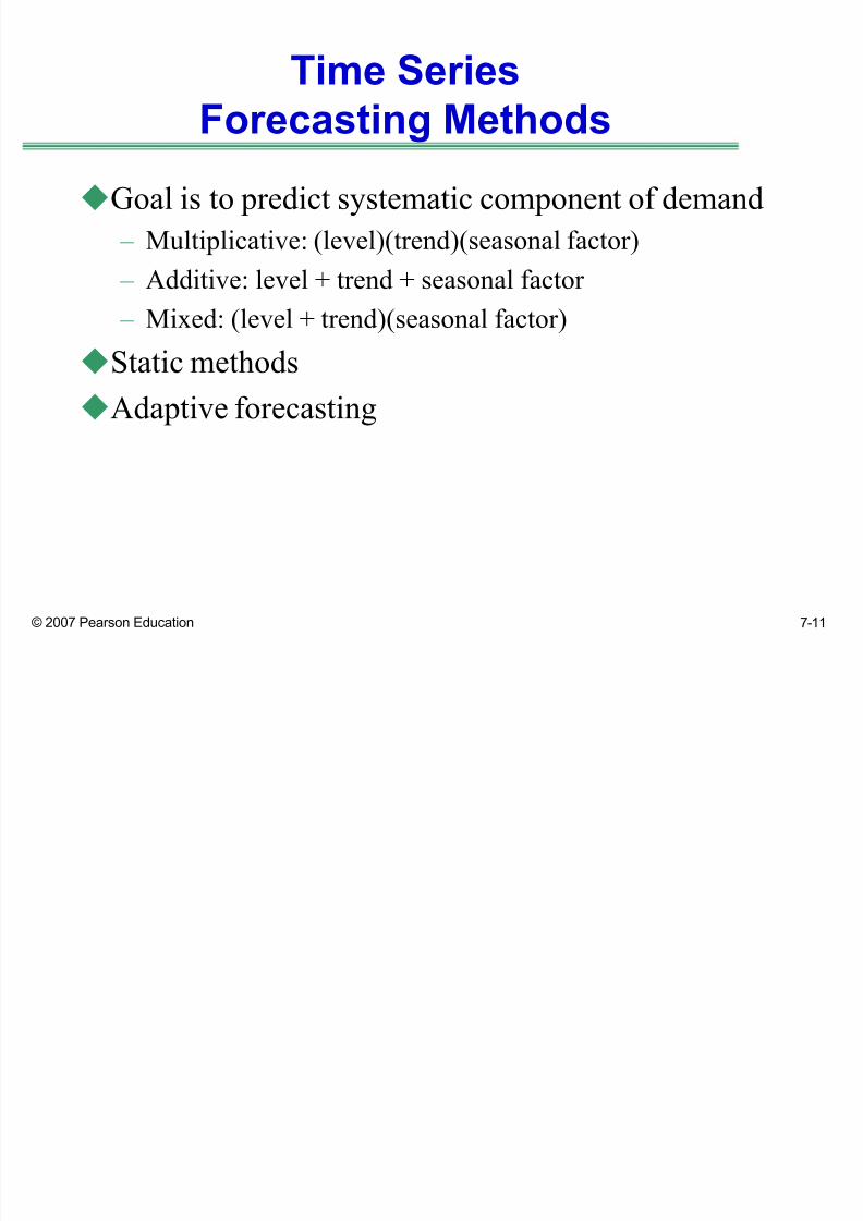
Goal is to predict systematic component of demand
± Multiplicative: (level)(trend)(seasonal factor)
± Additive: level + trend + seasonal factor
± Mixed: (level + trend)(seasonal factor)
Static methods
Adaptive forecasting
8/8/2019 Chopra3 Ppt Ch07
http://slidepdf.com/reader/full/chopra3-ppt-ch07 12/43
© 2007 Pearson Education 7-12
Static Methods
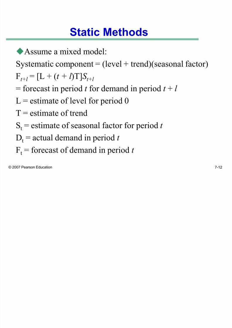
Assume a mixed model:
Systematic component = (level + trend)(seasonal factor)
Ft+l
= [L + (t + l )T]S t+l
= forecast in period t for demand in period t + l
L = estimate of level for period 0
T = estimate of trend
St = estimate of seasonal factor for period t
Dt = actual demand in period t
Ft = forecast of demand in period t

8/8/2019 Chopra3 Ppt Ch07
http://slidepdf.com/reader/full/chopra3-ppt-ch07 13/43
© 2007 Pearson Education 7-13
Static Methods
Estimating level and trend
Estimating seasonal factors

8/8/2019 Chopra3 Ppt Ch07
http://slidepdf.com/reader/full/chopra3-ppt-ch07 14/43
© 2007 Pearson Education 7-14
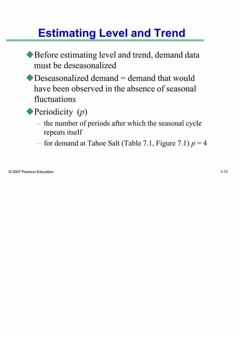
Estimating Level and Trend
Before estimating level and trend, demand data
must be deseasonalized
Deseasonalized demand = demand that would
have been observed in the absence of seasonal
fluctuations
Periodicity ( p)
± the number of periods after which the seasonal cyclerepeats itself
± for demand at Tahoe Salt (Table 7.1, Figure 7.1) p = 4

8/8/2019 Chopra3 Ppt Ch07
http://slidepdf.com/reader/full/chopra3-ppt-ch07 15/43
© 2007 Pearson Education 7-15
Time Series Forecasting
(Table 7.1)
Quarter Demand Dt
II, 1998 8000
III, 1998 13000
IV, 1998 23000
I, 1999 34000II, 1999 10000
III, 1999 18000
IV, 1999 23000
I, 2000 38000II, 2000 12000
III, 2000 13000
IV, 2000 32000
I, 2001 41000
F orecast demand for the
next four quarters.

8/8/2019 Chopra3 Ppt Ch07
http://slidepdf.com/reader/full/chopra3-ppt-ch07 16/43
© 2007 Pearson Education 7-16
Time Series Forecasting
(Figure 7.1)
0
10,000
20,000
30,000
40,000
50,000
9 7 , 2
9 7 , 3
9 7 , 4
9 8 , 1
9 8 , 2
9 8 , 3
9 8 , 4
9 9 , 1
9 9 , 2
9 9 , 3
9 9 , 4
0 0 , 1
8/8/2019 Chopra3 Ppt Ch07
http://slidepdf.com/reader/full/chopra3-ppt-ch07 17/43
© 2007 Pearson Education 7-17
Estimating Level and Trend
Before estimating level and trend, demand data
must be deseasonalized
Deseasonalized demand = demand that would
have been observed in the absence of seasonal
fluctuations
Periodicity ( p)
± the number of periods after which the seasonal cyclerepeats itself
± for demand at Tahoe Salt (Table 7.1, Figure 7.1) p = 4

8/8/2019 Chopra3 Ppt Ch07
http://slidepdf.com/reader/full/chopra3-ppt-ch07 18/43
© 2007 Pearson Education 7-18
Deseasonalizing Demand
[Dt-(p/2)
+ Dt+(p/2)
+ 7 2Di
] / 2p for p even
Dt = (sum is from i = t+1-(p/2) to t+1+(p/2))
7 Di / p for p odd
(sum is from i = t-(p/2) to t+(p/2)), p/2 truncated to lower integer

8/8/2019 Chopra3 Ppt Ch07
http://slidepdf.com/reader/full/chopra3-ppt-ch07 19/43
© 2007 Pearson Education 7-19
Deseasonalizing Demand
For the example, p = 4 is even
For t = 3:
D3 = {D1 + D5 + Sum(i=2 to 4) [2Di]}/8
= {8000+10000+[(2)(13000)+(2)(23000)+(2)(34000)]}/8
= 19750
D4 = {D2 + D6 + Sum(i=3 to 5) [2Di]}/8
= {13000+18000+[(2)(23000)+(2)(34000)+(2)(10000)]/8
= 20625

8/8/2019 Chopra3 Ppt Ch07
http://slidepdf.com/reader/full/chopra3-ppt-ch07 20/43
© 2007 Pearson Education 7-20
Deseasonalizing Demand
Then include trend
Dt = L + t T
where Dt = deseasonalized demand in period t
L = level (deseasonalized demand at period 0)
T = trend (rate of growth of deseasonalized demand)
Trend is determined by linear regression using
deseasonalized demand as the dependent variable and period as the independent variable (can be done in
Excel)
In the example, L = 18,439 and T = 524

8/8/2019 Chopra3 Ppt Ch07
http://slidepdf.com/reader/full/chopra3-ppt-ch07 21/43
© 2007 Pearson Education 7-21
Time Series of Demand
(Figure 7.3)
0
10000
20000
30000
40000
50000
1 2 3 4 5 6 7 8 9 10 11 12
Period
D e m a n Dt
Dt-bar

8/8/2019 Chopra3 Ppt Ch07
http://slidepdf.com/reader/full/chopra3-ppt-ch07 22/43
© 2007 Pearson Education 7-22
Estimating Seasonal Factors
Use the previous equation to calculate deseasonalized
demand for each period
St
= Dt
/ Dt
= seasonal factor for period t
In the example,
D2 = 18439 + (524)(2) = 19487 D2 = 13000
S2 = 13000/19487 = 0.67
The seasonal factors for the other periods are
calculated in the same manner

8/8/2019 Chopra3 Ppt Ch07
http://slidepdf.com/reader/full/chopra3-ppt-ch07 23/43
© 2007 Pearson Education 7-23
Estimating Seasonal Factors
(Fig. 7.4)
t Dt Dt-bar S-bar
1 8000 18963 0.42 = 8000/18963
2 13000 19487 0.67 = 13000/19487
3 23000 20011 1.15 = 23000/20011
4 34000 20535 1.66 = 34000/20535
5 10000 21059 0.47 = 10000/210596 18000 21583 0.83 = 18000/21583
7 23000 22107 1.04 = 23000/22107
8 38000 22631 1.68 = 38000/22631
9 12000 23155 0.52 = 12000/23155
10 13000 23679 0.55 = 13000/23679
11 32000 24203 1.32 = 32000/24203
12 41000 24727 1.66 = 41000/24727

8/8/2019 Chopra3 Ppt Ch07
http://slidepdf.com/reader/full/chopra3-ppt-ch07 24/43
© 2007 Pearson Education 7-24
Estimating Seasonal FactorsThe overall seasonal factor for a ³season´ is then obtained
by averaging all of the factors for a ³season´
If there are r seasonal cycles, for all periods of the form
pt+i, 1<i< p, the seasonal factor for season i isSi = [Sum(j=0 to r-1) S j p+i]/r
In the example, there are 3 seasonal cycles in the data and
p=4, so
S1 = (0.42+0.47+0.52)/3 = 0.47
S2 = (0.67+0.83+0.55)/3 = 0.68
S3 = (1.15+1.04+1.32)/3 = 1.17
S4 = (1.66+1.68+1.66)/3 = 1.67

8/8/2019 Chopra3 Ppt Ch07
http://slidepdf.com/reader/full/chopra3-ppt-ch07 25/43
© 2007 Pearson Education 7-25
Estimating the Forecast
Using the original equation, we can forecast the next
four periods of demand:
F13 = (L+13T)S1 = [18439+(13)(524)](0.47) = 11868
F14 = (L+14T)S2 = [18439+(14)(524)](0.68) = 17527
F15 = (L+15T)S3 = [18439+(15)(524)](1.17) = 30770
F16 = (L+16T)S4 = [18439+(16)(524)](1.67) = 44794

8/8/2019 Chopra3 Ppt Ch07
http://slidepdf.com/reader/full/chopra3-ppt-ch07 26/43
© 2007 Pearson Education 7-26
Adaptive Forecasting
The estimates of level, trend, and seasonality are
adjusted after each demand observation
General steps in adaptive forecasting
Moving average
Simple exponential smoothing
Trend-corrected exponential smoothing (Holt¶s
model)Trend- and seasonality-corrected exponential
smoothing (Winter¶s model)

8/8/2019 Chopra3 Ppt Ch07
http://slidepdf.com/reader/full/chopra3-ppt-ch07 27/43
© 2007 Pearson Education 7-27
Basic Formula for
Adaptive Forecasting
Ft+1 = (Lt + l T)St+1 = forecast for period t+l in period t
Lt = Estimate of level at the end of period t
Tt = Estimate of trend at the end of period t
St = Estimate of seasonal factor for period t
Ft = Forecast of demand for period t (made period t -1 or
earlier)
Dt = Actual demand observed in period t Et = Forecast error in period t
At = Absolute deviation for period t = |Et |
MAD = Mean Absolute Deviation = average value of At

8/8/2019 Chopra3 Ppt Ch07
http://slidepdf.com/reader/full/chopra3-ppt-ch07 28/43
© 2007 Pearson Education 7-28
General Steps in
Adaptive Forecasting
Initialize: Compute initial estimates of level (L0), trend
(T0), and seasonal factors (S1,«,S p). This is done as
in static forecasting.
Forecast: Forecast demand for period t+1 using thegeneral equation
Estimate error: Compute error Et+1 = Ft+1- Dt+1
Modify estimates: Modify the estimates of level (Lt +1),trend (Tt +1), and seasonal factor (St+ p+1), given the
error Et +1 in the forecast
Repeat steps 2, 3, and 4 for each subsequent period

8/8/2019 Chopra3 Ppt Ch07
http://slidepdf.com/reader/full/chopra3-ppt-ch07 29/43
© 2007 Pearson Education 7-29
Moving Average
Used when demand has no observable trend or seasonality
Systematic component of demand = level
The level in period t is the average demand over the last N
periods (the N-period moving average)
Current forecast for all future periods is the same and is based
on the current estimate of the level
Lt = (Dt + Dt-1 + « + Dt-N+1) / N
Ft+1 = Lt and Ft+n = Lt
After observing the demand for period t +1, revise the
estimates as follows:
Lt+1 = (Dt+1 + Dt + « + Dt-N+2) / N
Ft+2 = Lt+1

8/8/2019 Chopra3 Ppt Ch07
http://slidepdf.com/reader/full/chopra3-ppt-ch07 30/43
© 2007 Pearson Education 7-30
Moving Average Example
From Tahoe Salt example (Table 7.1)
At the end of period 4, what is the forecast demand for periods 5
through 8 using a 4-period moving average?
L4 = (D4+D3+D2+D1)/4 = (34000+23000+13000+8000)/4 = 19500F5 = 19500 = F6 = F7 = F8
O bserve demand in period 5 to be D5 = 10000
Forecast error in period 5, E5 = F5 - D5 = 19500 - 10000 = 9500
Revise estimate of level in period 5:L5 = (D5+D4+D3+D2)/4 = (10000+34000+23000+13000)/4 =
20000
F6 = L5 = 20000

8/8/2019 Chopra3 Ppt Ch07
http://slidepdf.com/reader/full/chopra3-ppt-ch07 31/43
© 2007 Pearson Education 7-31
Simple Exponential Smoothing
Used when demand has no observable trend or seasonality
Systematic component of demand = level
Initial estimate of level, L0, assumed to be the average of all
historical dataL0 = [Sum(i=1 to n)Di]/n
Current forecast for all future periods is equal to the current
estimate of the level and is given as follows:
Ft+1 = Lt and Ft+n = Lt
After observing demand Dt+1, revise the estimate of the level:
Lt+1 = EDt+1 + (1-E)Lt
Lt+1 = Sum(n=0 to t+1)[E(1-E)nDt+1-n ]
8/8/2019 Chopra3 Ppt Ch07
http://slidepdf.com/reader/full/chopra3-ppt-ch07 32/43
© 2007 Pearson Education 7-32
Simple Exponential Smoothing
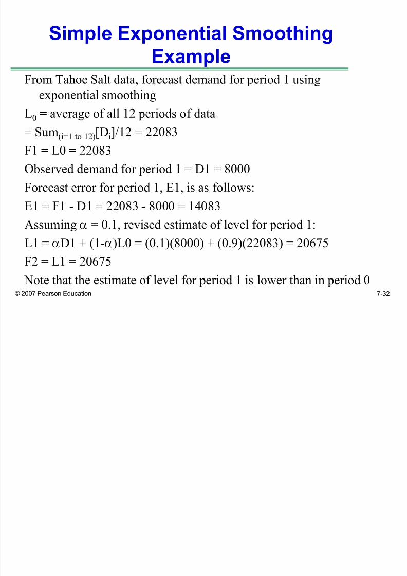
ExampleFrom Tahoe Salt data, forecast demand for period 1 using
exponential smoothing
L0 = average of all 12 periods of data
= Sum(i=1 to 12)[Di]/12 = 22083
F1 = L0 = 22083
O bserved demand for period 1 = D1 = 8000
Forecast error for period 1, E1, is as follows:
E1 = F1 - D1 = 22083 - 8000 = 14083
Assuming E = 0.1, revised estimate of level for period 1:
L1 = ED1 + (1-E)L0 = (0.1)(8000) + (0.9)(22083) = 20675
F2 = L1 = 20675
Note that the estimate of level for period 1 is lower than in period 0

8/8/2019 Chopra3 Ppt Ch07
http://slidepdf.com/reader/full/chopra3-ppt-ch07 33/43
© 2007 Pearson Education 7-33
Trend-Corrected Exponential
Smoothing (Holt¶s Model)
Appropriate when the demand is assumed to have a level and
trend in the systematic component of demand but no seasonality
O btain initial estimate of level and trend by running a linear
regression of the following form:Dt = at + b
T0 = a
L0 = b
In period t, the forecast for future periods is expressed as follows:Ft+1 = Lt + Tt
Ft+n = Lt + nTt

8/8/2019 Chopra3 Ppt Ch07
http://slidepdf.com/reader/full/chopra3-ppt-ch07 34/43
© 2007 Pearson Education 7-34
Trend-Corrected Exponential
Smoothing (Holt¶s Model)
After observing demand for period t, revise the estimates for level
and trend as follows:
Lt+1 = EDt+1 + (1-E)(Lt + Tt)
Tt+1 = F(Lt+1 - Lt) + (1- F)Tt
E = smoothing constant for level
F = smoothing constant for trend
Example: Tahoe Salt demand data. Forecast demand for period 1
using Holt¶s model (trend corrected exponential smoothing)Using linear regression,
L0 = 12015 (linear intercept)
T0 = 1549 (linear slope)
8/8/2019 Chopra3 Ppt Ch07
http://slidepdf.com/reader/full/chopra3-ppt-ch07 35/43
© 2007 Pearson Education 7-35
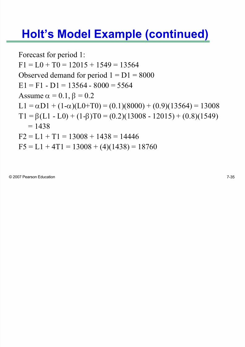
Holt¶s Model Example (continued)
Forecast for period 1:
F1 = L0 + T0 = 12015 + 1549 = 13564
O bserved demand for period 1 = D1 = 8000
E1 = F1 - D1 = 13564 - 8000 = 5564Assume E = 0.1, F = 0.2
L1 = ED1 + (1-E)(L0+T0) = (0.1)(8000) + (0.9)(13564) = 13008
T1 = F(L1 - L0) + (1- F)T0 = (0.2)(13008 - 12015) + (0.8)(1549)
= 1438F2 = L1 + T1 = 13008 + 1438 = 14446
F5 = L1 + 4T1 = 13008 + (4)(1438) = 18760

8/8/2019 Chopra3 Ppt Ch07
http://slidepdf.com/reader/full/chopra3-ppt-ch07 36/43
© 2007 Pearson Education 7-36
Trend- and Seasonality-Corrected
Exponential Smoothing
Appropriate when the systematic component of
demand is assumed to have a level, trend, and seasonal
factor
Systematic component = (level+trend)(seasonal factor)Assume periodicity p
O btain initial estimates of level (L0), trend (T0),
seasonal factors (S1
,«,S p
) using procedure for static
forecasting
In period t, the forecast for future periods is given by:
Ft+1 = (Lt+Tt)(St+1) and Ft+n = (Lt + nTt)St+n

8/8/2019 Chopra3 Ppt Ch07
http://slidepdf.com/reader/full/chopra3-ppt-ch07 37/43
© 2007 Pearson Education 7-37
Trend- and Seasonality-Corrected
Exponential Smoothing (continued)
After observing demand for period t+1, revise estimates for level,
trend, and seasonal factors as follows:
Lt+1 = E(Dt+1/St+1) + (1-E)(Lt+Tt)
Tt+1 = F(Lt+1 - Lt) + (1- F)Tt
St+p+1 = K(Dt+1/Lt+1) + (1-K)St+1
E = smoothing constant for level
F = smoothing constant for trend
K = smoothing constant for seasonal factor Example: Tahoe Salt data. Forecast demand for period 1 using
Winter¶s model.
Initial estimates of level, trend, and seasonal factors are obtained
as in the static forecasting case

8/8/2019 Chopra3 Ppt Ch07
http://slidepdf.com/reader/full/chopra3-ppt-ch07 38/43
© 2007 Pearson Education 7-38
Trend- and Seasonality-Corrected
Exponential Smoothing Example (continued)
L0 = 18439 T0 = 524 S1=0.47, S2=0.68, S3=1.17, S4=1.67
F1 = (L0 + T0)S1 = (18439+524)(0.47) = 8913
The observed demand for period 1 = D1 = 8000
Forecast error for period 1 = E1 = F1-D1 = 8913 - 8000 = 913
Assume E = 0.1, F=0.2, K=0.1; revise estimates for level and trend
for period 1 and for seasonal factor for period 5
L1 = E(D1/S1)+(1-E)(L0+T0) = (0.1)(8000/0.47)+(0.9)(18439+524)=18769
T1 = F(L1-L0)+(1- F)T0 = (0.2)(18769-18439)+(0.8)(524) = 485S5 = K(D1/L1)+(1-K)S1 = (0.1)(8000/18769)+(0.9)(0.47) = 0.47
F2 = (L1+T1)S2 = (18769 + 485)(0.68) = 13093
8/8/2019 Chopra3 Ppt Ch07
http://slidepdf.com/reader/full/chopra3-ppt-ch07 39/43
© 2007 Pearson Education 7-39
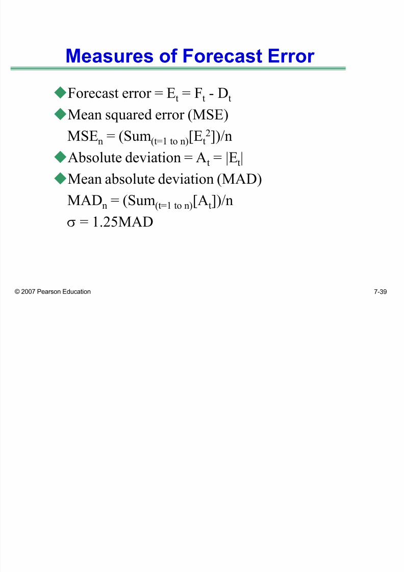
Measures of Forecast Error
Forecast error = Et = Ft - Dt
Mean squared error (MSE)
MSEn
= (Sum(t=1 to n)
[Et
2])/n
Absolute deviation = At = |Et|
Mean absolute deviation (MAD)
MADn = (Sum(t=1 to n)[At])/n
W = 1.25MAD

8/8/2019 Chopra3 Ppt Ch07
http://slidepdf.com/reader/full/chopra3-ppt-ch07 40/43
© 2007 Pearson Education 7-40
Measures of Forecast Error
Mean absolute percentage error (MAPE)
MAPEn = (Sum(t=1 to n)[|Et/ Dt|100])/n
Bias
Shows whether the forecast consistently under- or
overestimates demand; should fluctuate around 0
biasn = Sum(t=1 to n)[Et]
Tracking signal
Should be within the range of +6
Otherwise, possibly use a new forecasting method
TSt = bias / MADt

8/8/2019 Chopra3 Ppt Ch07
http://slidepdf.com/reader/full/chopra3-ppt-ch07 41/43
© 2007 Pearson Education 7-41
Forecasting Demand at Tahoe Salt
Moving average
Simple exponential smoothing
Trend-corrected exponential smoothing
Trend- and seasonality-corrected exponential
smoothing

8/8/2019 Chopra3 Ppt Ch07
http://slidepdf.com/reader/full/chopra3-ppt-ch07 42/43
© 2007 Pearson Education 7-42
Forecasting in Practice
Collaborate in building forecasts
The value of data depends on where you are in the
supply chain
Be sure to distinguish between demand and sales

8/8/2019 Chopra3 Ppt Ch07
http://slidepdf.com/reader/full/chopra3-ppt-ch07 43/43
© 2007 Pearson Education 7-43
Summary of Learning Objectives
What are the roles of forecasting for an enterprise and
a supply chain?
What are the components of a demand forecast?
How is demand forecast given historical data using
time series methodologies?
How is a demand forecast analyzed to estimate
forecast error?