


Languages
Pages
Legal

CHEBYSHEV APPROXimTIONS
by
• PHILLIP F. UNRUH
B. A,, Kansas State University, 196?
A MASTER'S REPORT
submitted in partial fulfillment of the
requirements for the degree
MASTER OF SCIENCE
Department of Mathematics
KANSAS STATE UNIVERSITYManhattan, Kansas
r *' ^ 1968 : \ "*
\
Approved by:
*.
»
'<• '-
'-^LMajor Professor
R^ . ;.:-.
'^ ' - : . ,- TABLE OF CONTENTS
PageINTRODUCTION 1
PROPERTIES OP CHEBYSHEV POLYNOMIALS 2
N"*^^ DEGREE LEAST-SQUARES POLYNOMIAL APPROXniATION 11
THE "MINII-LAK" PRINCIPLE . ll^
ECONOMIZATION OP POTTER SERIES I7
CONCLUSION 26
ACKNOliTLEDGMENT 2?
REPERENCES 28
"" *.^
INTRODUCTION
The purpose of this report is the development of some of
the properties and applications of Chebyshev polynomials. This
class of functions was named after the Russian mathematician,
P. P. Chebyshev (l821-l89l|-) . Many papers and books dealing with
one or more characteristics of Chebyshev polynomials have been
written. .i: •
•
Chebyshev polynomials can be obtained in a variety of ways.
These polynomials include the eigenvalue-eigenfimction solutions
of a certain differential equation, generating functions,
Rodrigues-type formula, recursion formula, trigonometric defi-
nition, orthogonality definition, etc. Some of these deriva-
tions are discussed in this report. The various definitions -.
lead to the same set of functions, to v;ithin a multiplicative
constant. VJhenever we need to prove some relation, we use that
definition or property V7hich is most suitable and most easily
applied.
The two properties of Chebyshev polynomials which have
spurred their utilization are their Fourier Series property
(least-squares approximation) and their rainimax property. Both
of these are discussed in the report. In addition, they also
enter into considerations of continued fraction approximation
of functions. Trimcated continued fractions lead to Fade' ap-
proximants, the use of is generally considered to be a very
efficient approximative method.
PROPERTIES OP CHEBYSHEV POLYIIOMIALS
: Many techniques exist for finding polynomial approxima-
tions which reduce the amount of work and guarantee a specified
accuracy. The Chebyshev polynomials form a set which are among
the simplest and most useful of all polynomial approximations.
The Chebyshev polynomial of degree n can be defined by
Tn(35^) ~ cos{n arccos x). ' "\
If we set e = arc cos x, then T^^Cx) = cos ne. By using de
Moivre's theorem,
(cos e 4 i sin e)^ = cos ne + i sin no,
and noting that
sin © = (1 - cos e)*^ = (1 - x )'^,
we have
[x- id - x2)^]"'•
« x^ + nx^-^ [i{l-x2)'^] 4 n(n-l)x^-^ [id-x^)'^] ^ ^ ...
Then, by simplifying and taking the real part only of the ex-
pansion, we obtain
T„(x)= x^ + n(n-l) x""^(x^-l) + nCn-l) (n-2) (n-3) x'^"^(x^-l)^ + ...n21 TfT
Prom T (x) = cos(n arccos x) = cos ne, we can develop the
reciirrenco relation
T^^l(x) = 2xT^(x) - ViCx).
Since x = cos g, -1 f- x j^ 1, and -v < est we have that
T , (x) = cos(n4l)e = cos ne cos e - sin ne sin e
and
Tj^_-j^(x) " cos(n-l)© =: cos ne cos e + sm no sm e
Adding, yields
^n+1^^^ "* ^n-1^^^ ' ^°°^ ^® °°^ e » 2x T^(x);
hence
T^^l(x) . 2xT^(x) - Vi(x).
¥e can tabulate the Chebyshov polynomials from
Tjj(x) = cos ne
yielding
Tq(x) = coso = 1
and
T-, (x) = cos© = X, for n = 0,1.
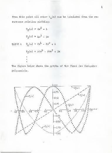
Prom this point all other T (x) can be tabulated from the re-
ciorrence relation yielding:
T^U) = 2x^-1
TABLE A T. (x) = 8x^ - 8x^ 4 1
T^(x) = I6x^ - 20x^ + 5x
The figure below shows the graphs of the first few Chebyshev
polynomials.
XX.X-.
X-.
X-.X '.
X •.
X •
XXXXXX
_x X
-1.6^-0.8 \-0,6
^r^^ TT^m^oo
o ^
ooo
-0.75 X
ooo
toXoXo Xo Xooooooo
o°/
XXXXX ^
/ X
X oX oXXX
^rQ(x) ^i
yy
_L
XXX^
yy
y XX
XX
X
?.
>•
XxX'
oo
0.50
1-0.25
y
/z*^/-,!/)
_L-0.2 /y
Ux\
<K/
X /X /x/
y x*-^(/)XX,
. oX^x
O Xox
o°XI n y L
% 0.2
o
1--0.25oo
l--0.50°o
—0.75
--1.00
XX
0.6 •• 0.8° X 1.0° Xo
o Xo Xo X° Xo ^
o Xo X
'^XXX
o ^XvXA°
The Chebyshev polynomials can bo shovm to satisfy the dif-
ferential equation
(1 . x2)^fy . X II * n2y =
This equation can be modified so as to conform with the Sturm-
Liouville form of the differential equation
on some interval a f x £ b, satisfying certain boundary condi-
tions by dividing by (1 - x ) ^.
In fitting the differential equation to the Sturra-Liouville
second-order differential equation above we note that
(x) = Vl- x^, q(x) =0, ^= n , p(x) =
the range is f-l, ij •
The equation takes the form
^ and
da:x /rr?i] -^ . = 0.
We note that for x = -1, r(x) = 0. Hence this problem has the
trivial solution y = for any value of the parameter A - n .
Solutions y, not identically zero, are called character-
istic functions or eigenfionctions of the problem, and the values
of A for vrhich such solutions exist, are called characteristic
values or eigenvalues of the problem.
Therefore [(1) PP. \i}\.-\\$\ the solutions corresponding
to different values of n form an orthogonal set over [-1, l]
1 *••'
with respect to the weight function /r~~~2.
To solve the differential equation, we can assume a pox-jer
series development, for each n » 0, 1, 2, . . , we obtain both
a polynomial and an infinite series, the polynomial solutions,
except for constant factors, are Chebyshev polynomials y = T (x)
for n = 0, 1, 2, . . .
.
The Chebyshev polynomials also can be shown to be identical
with the functions obtained from Rodrigues formula [(6), pp. 15-
A generating function for the Chebyshev polynomial is
^ - ^P
= fT^(x)u^1 - 2xu + u^ fzi
This generating function is derived from the geometric series
by noting that
1 _^ = 1le 1-ucose - iusine
1 - ue
1 - u cos + iu sin ©_ .__ ,
(1 - ucose) f u sin e
Taking the real parts yields
0-3
^ U Owa iiM — -.,
n-:.o 1 - 2u cos© -t u*cos n© = 1 - ^<^ogQ
Now, the standard substitution of x = cos © shows that the pre-
ceding function does generate the Chebyshev polynomials.
Prom the polynomials preceding, it is easily seen that the
leading term of T^^Cx) for n>l is 2""-'-x^. Chebyshev polynomi-
als, T (x), have simple zeros at the n points x^^ «• cos^rx
'^'
k = 1, 2, . . . n. This is seen by substituting x^^ in T^Cxj^) =
cos(n arccos x) . Hence:
Tjj(x^) = cosfn arccos (cos -I—*")]= cos ~^^ ^
for k «= 1, 2, . . . n.
Then T'(x) = -sin(n arccos x) -JiJL. a j«£—^ sin(^ arccos x)
.
"/l-x^ VI-x^
Therefore T^(xj^) = ;=^«2 ^^^ ^^tt f implies that the zeros
must be simple. This can also be seen on observing that the
degree of Tj^(x) is n; therefore, Tj^(x) has exactly n zeros.
Also the zeros must be simple since Tj^(x) has n different zeros,
Another useful property of T (x) is that its extreme val-
k<»ues are - 1, These n + 1 values are obtained for x^ = cos -T/*
k kFrom the proof above, T' (xA) = n(l-cos ^)
'^ sinkw = for k =
1, 2, .. , . n-1. Then T^(x^) = cosfn arccos ( cos- tj)] = cos k» =
(-1) for k = 0, 1, . . . n. But since -1 < x £ 1, T^(x) = cos
(n arccos x) implies that|Tj^(x]^ £ 1. Hence this shovrs that the
values xA give extreme values.
8
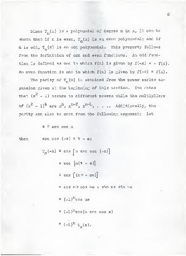
Since T (x) is a polynomial of degree n in x, it can be
shown that if n is even, Tj^(x) is an even polynomial; and if >
n is odd, T (x) is an odd polynomial. This property follovrs
from the definition of odd and even fimctions. An odd func-
tion is defined as one in v;hich f(x) is given by f(-x) = - f(x).
An even fxmction is one in x^rhich f(x) is given by f(-x) = f(x).
The parity of T (x) is obtained from the power series ex-
pansion given at the beginning of this section. One notes
that (x - 1) occurs to different powers v^hile the multipliers
of (x^ - 1)^ are x^, x^"^, x^"^, .... Additionally, the
parity can also be seen from the following argument: let
© = arc cos x
then arc cos (-x) = tt - g;
Tj^(-x) = cos fn arc cos (-x)"]
= cos [n(Tr - g)] .
'
^^
= cos [^(mi - n©)j
= cos n7] cos ne + sin ni) sin ne
• ' = (-l)^cos ne ,
= (-l)^cos(n arc cos x)
= (-1)^ T^(x).
/
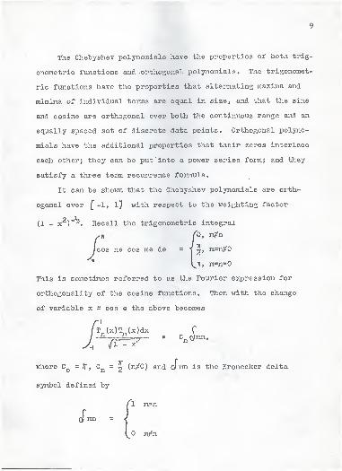
The Chebyshev polynomials have the properties of both trig-
onometric fiinctions and orthogonal polynomials. The trigonomet-
ric functions have the properties that alternating maxima and
minima of individual terms are equal in size, and that the sine
and cosine are orthogonal over both the continuous range and an
equally spaced set of discrete data points. Orthogonal polyno-
mials have the additional properties that their zeros interlace
each other; they can be put into a power series form; and they
satisfy a three term recurrence fonaula.
It can be shown that the Chebyshev polynomials are orth-
ogonal over f-1, 1} with respect to the weighting factor
(1 - X )"'^. Recall the trigonometric integral
cos ne cos m© de ""f 2*
^~^^^ "•
',
V^u, m=ns:0
This is sometimes referred to as the Fourier expression for
orthogonality of the cosine functions. Then with the change
of variable x = cos © the above becomes t ,
ITT^)j^<)mn.
T^(x)Tj^(x)dx \;.--..
where C^ = TT, C^^ = ^ (^7^0) and ol ran is the Kronecker delta
symbol defined by
^man
ran
m/n
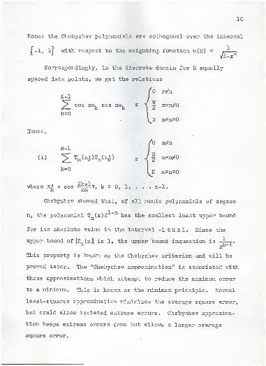
V. _ j; ^ .: 10
Hence the Chebyshev polynomials are orthogonal over the interval
f-l, If with respect to the weighting function w(x) = i==»«ry
'
, Correspondingly, in the discrete domain for N equally
spaced data points, we get the relations
m/nN-1
nna ^-^^ ^yjci ll'^Tj.
k=0
cos me^, cos n©,, = a ^ m=n;^0
N m=n=0
Hence,
"O mj^nN-1
^''^. \ N ra=n=0
Where 2^ = cos '
^xi ' k = 0, 1, . . . n-1.
Chebyshev showed that, of all monic polynomials of degree
n, the polynomial T (x)2 *" has the smallest least upper bound
for its absolute value in the interval -1 £ x < 1 . Since the
upper bound of JT (x^ is 1, the upper bound inquestion is ^
.
This property is known as the Chebyshev criterion and will be
proved later. The "Chebyshev approximation" is associated v;ith
those approximations v/hich attempt to reduce the maximum error
to a minimtmi. This is known as the minimax principle. Normal
least-squares approximation minimizes the average square error,
but could allow isolated extreme errors. Chebyshev approxima-
tion keeps extreme errors doim but allows a larger average
square error.
11
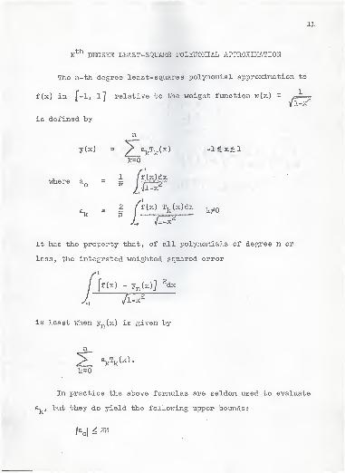
: N*^ DEGREE LEAST-SQUARE POLYITOMIAL APPROXIi-iATION
The n-th degree least-squares polynomial approximation to
f(x) in f-l, ll relative to the weight function v;(x) = /==^
is defined by
.
-- n .:
•
y(x) = Z^W^^^ -i^x£ik=0
I .-
1 /f(x)dxwhere a^ = ^ Ijf^ ^"A'^:
><.? "t.•
^2 /f(x) Tjjx)dx ^j,Q
It has the property that, of all polynomials of degree n or
less, the integrated weighted squared error
ff{x) - y^(x)] ^dx
a:x^
is least when yj,(x:) is given by
n _
a^T^(x)
k=0
In practice the above formulas are seldom used to evaluate
a^, but they do yield the following upper bounds:
Klif /lued. =!f
-j'! ;"'•• "A "^-^'i'"•'" ''"•
k ?
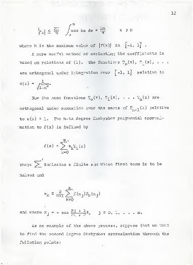
12
where M is the maximum value of )f (x)| in |_-1, IJ .
A more useful method of evaluating the coefficients is
based on relations of (1). The fvinctions Tq(x), T-^{x) , . . .
are orthogonal under integration over [-1» IJ relative to
•w(x) « /==^.yjl-x. '
Now the same f\anctions Tq(x), T-^Cx), . . . T^(x) are •
orthogonal under summation over the zeros of Tj^_i(x) relative
to w(x) = 1. The n-th degree Chebyshev polynomial approxi-
mation to f(x) is defined by
n ,
'(^' =ZVk(-'
/
where ^__ indicates a finite sum whose first term is to be
halved and '
"'''
n
. k=o .. ., .:
-
and where Xj » - cos |J *
^Tf, j = 0, 1, . . . n.
As an example of the above process, suppose that we want
to find the second degree Chebyshev approximation through the
folloTiring points:,
..
~: <.* %i
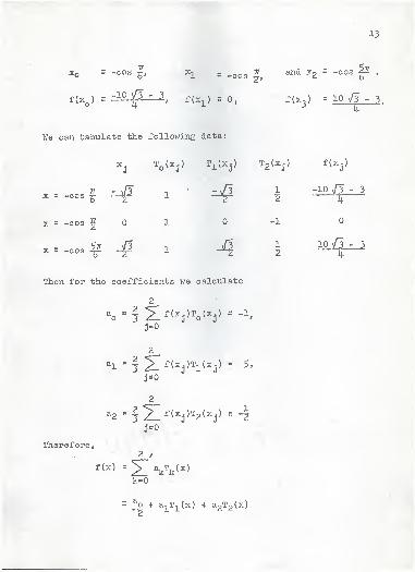
Y J!^^^ = -cos f, Xi = -COS |,and X2 = -COS |l
.
f(x^) = -^Q)[3
- 3^ f(^^) -
0^. f(x^) = 10 v^ - 3
We can tabulate the following data:
•v, ' x^ T^(Xj) Ti(Xj) TgUj) ' fUj) ;: .
Tf - v/I -, • zJl 1 -10/3-3X = -cos ^ _^ 1 -^ ^ )L^
X = -cos 5 1 -1 ,
^ - 5;? _i3 1 jH 1 10/3-3X - -cos ^ _|2 1 -^ 2
Ij;
Then for the coefficients we calciilate
2 -
^f(x )T^(x.) = -1,a = 2o 3 .il-.
-^^J' O^ J
J-0
^1 =f 2^^^^j)^l^^j^ - ^^
2
J-0
\
Therefore, \\ \j v "- . , . , ,
k-0
= ^o + a-^^T-^Cx) 4 a2T2(x)
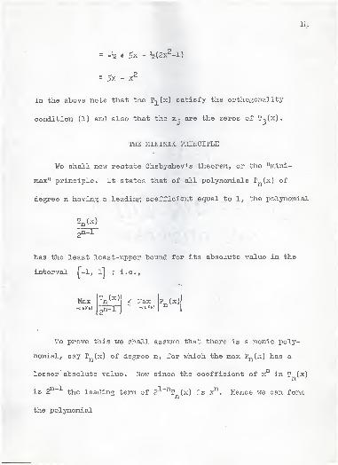
lil-
-h 4 5x - 3^2(2x^-1)
25x - X
In the above note that the T-]^(x) satisfy the orthogonality
condition (1) and also that the x. are the zeros of T-^Cx) . .
.;;. : THE HINIl-lAX PRIHCIPLE
VJe shall now restate Chebyshev's theorem, or the "mini-
Biax" principle. It states that of all polynomials Pj^(x) of
degree n having a leading coefficient equal to 1, the polynomial
,: !n(fi^
-V'"-
....
has the least least-upper bound for its absolute value in the
interval f-l, l7 ; i.e..
Maxl^n^^^
l^ I,lax P„(x)
To prove this we shall assume that there is a monic poly-
nomial, say Pj,{x) of degree n, for v/hich the max Pr>(x) has a
lesser' absolute value. Nox^r since the coefficient of x in T (x)
is 2^" the leading terra of 2 "'^T„(x) is x^. Hence we can formn'
the polynomial
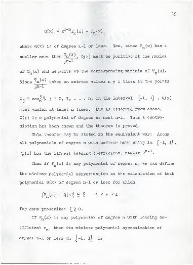
15
Q(x) = 2^-^T (x) - Tix) ^. ^'\
... - • ..A ^ ^. . ^ ,",..'.- --'' \ \
Where Q(x) is of degree n-1 or less. Now, since Pj^(x) has a
smaller norm than n^'^^ Q(x) must be positive at the maxima
of T^(x) and negative at the corresponding minimia of T^(x).
Siiice ^n^^^ takes on extreme values n + 1 times at the points
^ ,. 2^-1
X. = cos-ij^, j = 0, 1, . . . n, in the interval [-1, l] , Q(x)
must vanish at least n times. But as observed from above,
Q(x) is a polynomial of degree at most n-1. Thus a contra-
diction has been shovna and the theorem is proved.
This theorem may be stated in the equivalent way: Among
all polynomials of degree n with maximum norm unity in [-1, l] ,
T (x) has the largest leading coefficient, namely 2 ".
Thus if Pj,(x) is any polynomial of degree n, we can define
the minimax polynomial approximation as the calculation of that
polynomial Q(x) of degree n-1 or less for v/hich
(Pn(x) - Q(x)| 5 f.-1 £ X ^ 1
for some prescribed £ ^ 0.
^ .' If Pj,(3c) is any polynomial of degree n vrith leading co-
efficient a , then its minimax polynomial approximation of
degree n-1 or less on f-l* 1? is
16
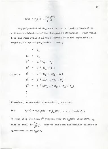
Any polynomial of degree n can be uniquely expressed as
a linear combination of the Chebyshev polynomials. From Table
A we can form Table B in which powers of x are expressed in
terms of Chebyshev polynomials. Thus,
^o
y
TABLE B
X = Tq^
jZ ^ 2-l(To + Tg)
j3 „2~^(3T-L * T3)
X^ = 2-3(3T^ + i^T2 * \)
x^ = 2"^(10Ti + 5T3 + T^)
yP = 2"^(10Tq + I5T2 + ^\ <- T^)\
Therefore, there exist constants C-,^ such that
(6) Pj^(x) = CoTqCx) + C-lT^Cx) + . . . + C^TnCx).
We note that the term x^ appears only in Tj^(x) ; therefore, C
a^must be equal to ^. Thus we can form the miniraax polynomial
pn~JL
approximation to Pj,^^^*
17
(7) Q(x) = C^ + C^T-^M f C2T2(x) 4 ... - Cj^_iTn_l(x).
Therefore, v;e see that to obtain the rainiitiax polynomial
approximation to a given polynomial ?^{x.) we first express Pn(x)
as the series (6) of Chebyshev polynomials and then drop the
last term,
ECONOMIZATION OP PO^VER SERIES
It txirns out that in many cases one can drop more than one
term and still obtain approximations which are "close" to being
minimax, which we shall show later in an example illustrating
this method of approximating polynomials. In actual practice,
we need only retain the terms through some k, k<.n, in (6)
since |T:i(x)| ^1 for all j. In doing this, the error committedV
is bounded by '
.^
The procedure above for replacing a polynomial of given
degree by one of lower degree is sometimes referred to "econ-
omizing a power series". We shall outline this procedure for
obtaining an economized polynomial approximation to a function
f (x) belo;^.
The economization of a power series has four basic steps.
Step 1. Expand f(x) in a Taylor series valid on the interval
18
[-1, 1[ . Trimcate this series to obtain a polynomial
;":•;•-,«' > ^ .,-:
Pj^(x) = a^ 4 a-j^x + . . . -f a^x >-.. „-?
which approximates f (x) to within a prescribed tolerance error
C for all X in [-1, l] .
Step 2. Expand P_{x) in a Chebyshev seriesn
Pj^(x) = Cq + C^^T-j^Cx) •...+ CnTn(x)
making use of Table B.
Step 3. Retain the first k terms in this series
.=^ Mj5.(x) » Cq + ^1^1^^^ f . . . + Oy^T-^U)
choosing k so that the maximum error given by v
if(x) -i^^{x)\s e+ K,ii+ . . . + Ki
is acceptable. •
Step i}.. Replace T.(x), (j=0, l,..k) by its polynoradal form
using Table A and rearrange to obtain the economized polynomial
approximation of degree k in standard form,
f (x)c: c'^ + O-^TL - . . . + Cjj.x
If necessary in step 1, make a transformation of independent
variables so that the expansion is valid on that interval.
As an example of the above procedvire we shall find a
polynomial of as low a degree as possible vjhich vrill yield
19
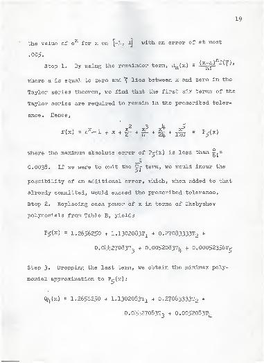
the value of e^ for x on [-1, l] with an error of at most
.005.
Stop 1. By using the remainder term, B.^{x) = ^'^^ ^V
>
where a is equal to zero and "^ lies between x and zero in the
Taylor series theorem, we find that the first six terms of the
Taylor series are required to remain in the prescribed toler-
ance. Hence,
"
S x3 x^, x^f(x) =e^-l + x + ^4i- + #n- + T^ " Pcr(x)
where the maximijun absolute error of P^(x) is less than -^.^
0.0038, If we were to omit the $y terra, we would inciu? the
possibility of an additional error, which, when added to that
already committed, would exceed the prescribed tolerance.
Step 2, Replacing each power of x in terms of Chebyshev
polynomials from Table B, yields
P5(x) = 1.2656250 + I.I302083T-L * O.27083333T2 •
O.Oi|li.27083To + 0.0052083Ti^ + 0.00052356t^
Step 3» Dropping the last term, v;e obtain the minimax poly-
nomial approximation to P^(x) : t- - '•
Qij^Cx) = 1.2656250 + 1.1302083T]_ + 0.27083333^2 +
0.0]4ij.27083T3 4 0.0052083T|^
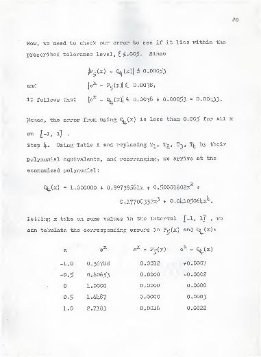
20
Now, we need to check our error to see if it lies within the
prescribed tolerance level, £ ^.005. Since
. Ip^U) - Qj^(x)| 6: 0.00053
and.
|e^ - 7^Ui^ 0.0038,
it follows that |e^ - Qh (x)( ^ O.OO38 + 0.00053 - O.OOi|.33.
Hence, the error from using Q^Cx) is less than 0.005 for all x
on [-1, 1] .-
Step 1].. Using Table A and replacing T]_, T2, T3, T[^ by their
polynomial equivalents, and rearranging, we arrive at the
economized polynomial:
Qi^(x) - 1.000000 + 0.99739581X t 0.5000l602x^ +
0.17708332x^ + 0.0iia0506Ipc^.
Letting x take on some values in the interval [-1, ly ,
can tabulate the corresponding errors in P^(x) and Qj. (x)
:
v/e
k^-r •: e^ :- i.' e^ - P^Cx) e^ - Qij^(x)
1.0 0.36788 * * 0.0012 f0.0007
0.5 0.60653 * 0.0000 -0.0002
1.0000 0.0000 0.0000
0.5 1.61j.87 0.0000 0.0003
1.0 2.7183 ', 0.0016 0.0022
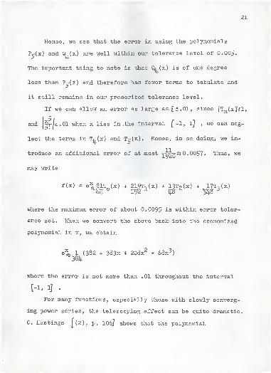
21
Hence, we see that the error in using the polynomials
Pi-(x) and Qk(x) are well within our tolerance level of 0.005.
The important thing to note is that Q^ (x) is of one degree
less than Pi-{x) and therefore has fewer terms to tabulate and
it still remains in our prescribed tolerance level.
If we can allov; an error as large as £5.01, since |T (x](^l,
and §r/<:.01 when x lies in .the interval f-1, l] , we can neg-
lect the terras in T^(x) and T^(x). Hence, in so doing, we in-
troduce an additional error of at most Tq "̂q ^ 0057 « Thus, v;e
may write
f(x) = e^8lT^(x) + 219Tt (x) * 13T2(x) + 17To(x)
where the maximum error of about 0.0095 is within error toler-
ance set, VJhen we convert the above back into the economized
polynomial in x, v;e obtain ..
e^ 1 (382 + 383x + 208x^ + 68x^) "^v
where the error is not more than .01 throughout the interval
[-1, ij . ;,-
For many functions, especially those with slowly converg-
ing power series, the telescoping effect can be quite dramatic.
C. Hastings [(2), p. 106? shows that the polynomial
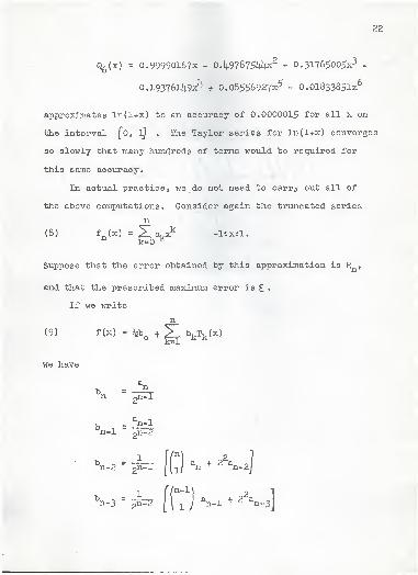
22
Q^(x) = 0.99990167X - 0.k.97Q7$kkjS + 0.3176^005x^ -
0.19376ll>.9x^ + 0.08556927x^ - O.Ol83385lx^
approximates ln(l+x) to an accuracy of 0.0000015 for all x on
the interval [o, ij . The Taylor series for ln(l+x) converges
so slowly that many hijndreds of terras wo\ild "be required for
this same accuracy.J
. *,;; -.
In actual practice, we do not need to carry out all of
the above computations. Consider again the truncated series
n'
(8) f„(x)=51a^x^ -I'.xil.
.;; *^ k=0 ^
Suppose that the error obtained by this approximation is R^^,
and that the prescribed maximiira error is £ •
If we write A
(9) f(x) = ^b^ + T. h^T^U) :
we have
^n - :3IT
^n-l - ^512
V2=^ y ^n + 22a.J
"n-S = i:2 1 ("i'l ^n-l *2'^«]
.yWBJpl.., . "^ ,
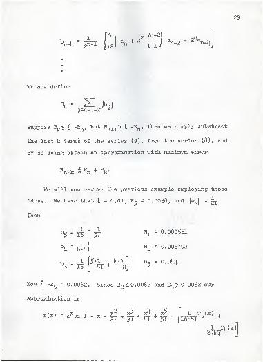
23
b - ^n-lj. pia-l
i2i^ -^ '^
Til "--2' ^^v
We now define .
n
^ j=n-l-k' J'
Suppose Bj^< C -Rn» ^^"^ ^+1^^ ^ "^n* *^®^ ^® siraply substract
the last k terras of the series (9), from the series (8), and
by so doing obtain an approximation with maximuim error
Vk ^^n -^ ^- ,: .
- 'V >/
We will now rei^-ork the previous example employing these
ideas. We have that [ = 0.01, R^ = O.OO38, and |aij| = ^^''"'
' 1 '•• " ' ^' ''
•
Ihen .'; > "v' ^ » •. '^
:
b^ = ^ • -ry Bj^ = 0.000521
\ =^ B2 = 0.005792 -^ ...
^3 K [ FT + JI] ^
Now £ -R^ = 0.0062. Since 62^0. 0062 and Bo > 0.0062 our
approximation is
i'(„\ - „x^ T _, :^ x^ ^ x^ ^ x^ . x^ 1 TAx) .f (X) - e ^ 1 + X t -2j -^ jr •*
IfT+ 5T " [16-^ ^ ^
^1 T|,(x)]
2k
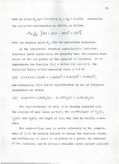
with an error Ro not exceeding R^ + B2 = 0.0095. Performing
the indicated substraction we obtain, as before,
^5^ 1 ["382 + 383X 4 208x^ 4 68x^]e^
with the maximum error Ro with the prescribed tolerance.
As the exponential function approximation indicates,
truncated power series have .the property that the maximum error
occurs at the end points of the interval of interest. If we
approximate the fijinction f{x) » sin^gvx for -li x 1 1, the
trxincated Taylor series expansion about x = is
(10) sin^Trx<*1.5708x - 0.6i^.60x^ 4 0.0797x^ - 0.00i|.7x'^.
Now economizing this series approximation by use of Chebyshev
polynomials we obtain .,
(11) sin^gTrxft 1.1336T3l(x) - 0.138lT2(x) 4 0.00I|.5T^(x) .
The representation of sin^g x is thereby achieved vrith
the storage of only three numbers, the coefficients of T-,(x),
T^(x), and Tk(x); the right of (11) may then be readily evalu-
ated .
The desk-machine user is seldom attracted by the compact-
ness of (11); he usually insists on seeing the function values
and differences in order to ascertain at a glance the behavior
of the function, and to obtain a reliable check against isolated
* V -At*, -k
/ r'*" ^..A
25
computing errors. However, for an automatic computer, which
is much less prone to isolated errors, the Chebyshev series
representation is preferable.
In this particular example, we note that the Taylor series
expansion has one more term than (11); if the Taylor series is
truncated after the third term, its maximum error is larger than
that for series (11).
This is a simple example of the general property that, in
a given finite range, an approximation in Chebyshev series of
prescribed degree represents a function of a real variable more
accurately than a truncated Taylor series of the same degree.
In the special case where the function happens to be a poly-'
nomial of the required degree, the Chebyshev and Taylor repre-
sentations are equally accurate, each being a rearrangement of
the other. Moreover, any fionction which can be represented by
an orthodox single-entry table can be represented by a single
Chebyshev series, whereas a Taylor series valid over the \ihole
tabular range may not exist. . ," "
We may summarize by restating that a trimcated Chebyshev
series is normally a good approximation to the best polynomial
representation in the sense of Chebyshev' s criteria. However,
it transpires that in practical applications the truncated
Chebyshev series is usually very close to the best possible
polynomial; the refinements necessary to improve it are seldom
worthwhile.
CONCLUSION'. / •
"
V In conclusion, in this report \iq have defined the Chebyshev
polynomials by means of the relation T^(x) = cos(n arccos x)
.
We have shown how they satisfy certain differential equations
arising from the solution of the Sturm-Liouville problem. Also,
we have shoxm that they can be obtained from a particular gen-
erating function, a Rodrigues-type formula, and a three terra
recurrence relation. V7e have shown that Chebyshev polynomials
are orthogonal over f-l, Ij v/ith respect to a certain v/eight
factor. They also possess the useful property that |t^(x)| £ 1
and Tj^(x) obtains its extreme values alternately of (-1) at
n f 1 points over the interval [-1, IJ •
We have utilized the Fourier Series property that the
Pourier-Chebyshev series minimizes the average square error.
An example is given to illustrate this idea. One of the most
important properties discussed in this report leads to the
minimax principle, along with the proof and an example to fit
the principle. Then from the minimax principle, the economi-
zation of power series was developed and it was shown that
certain fianctions can be evaluated numerically by this econo-
mizing process. The study of Chebyshev polynomials leads to
many interesting mathematical problems.
.;. ACKNOWLEDGl-IENT
The writer wishes to express his sincere appreciation
to Dr. S. T. Parker for introducing him to this subject and
for his patient guidance and supervision given diiring the
preparation of this report. .;
O i
/ i. *».•••- r r H
"-S
REFERENCES
ChTirchill, R. V.Fourier Series and Boundary Value Problems. McGraw-HillBook Company, 19l\.l, pp. l\l\.-lJi.S»
Conte, S. D.. Elementary N-uraerical Analysis. McG-ravj-Hill Book Company,1965, pp. 100-107.
Davis, Philip J.Interpolation and Approximation, Blaisdell PublishingCompany, I963, pp. 60-6I|..
Kelly, Louis G-.
Handbook of Numerical Methods and Applications. Addison-Wesley Publishing Company, 196?, PP. 76-80.^ , ,,,
Lanczos, Cornelius,Applied Analysis, Prentice Hall, Inc., 1956, VI>* I78-I8O,pp. i].5ij--i^.63.
,.
Snydner, Martin Avery. "" •"• ' ''
.'
Chebyshev Methods in Numerical Approximation. Prentice-Hall, Inc., 1966, pp. 11-lj.O.
CHEBYSHEV APPROXIMTIONS
by
PHILLIP P. UNRUH
B. A., Kansas State University, 196?
AN ABSTRACT OP A MASTER'S REPORT
submitted in partial fulfillment of the
requirements for the degree
MASTER OP SCIENCE
Department of Mathematics
KANSAS STATE milVERSITYManhattan, Kansas
1968 -'
r
i ':•.
V,. %
The name "Chebyshev polynomials" is in honor of the Russian
mathematician P. P. Chebyshev (l821-l89ii.) . Most of his contri-
butions to mathematics Mere in the area of number theory.
In this report the basic definition of the Chebyshev poly-
nomials we have employed is given by Tj^(x) = cos(n arccos x)
.
\Ie have shown how they satisfy certain differential equations
arising from the solution of a specific Sturm-Liouville problem.
Also, we have shown that they can be obtained from a particiilar
generating function, a Rodrigues-type formula, and a three term
recurrence relation. We have shown that Chebyshev polynomials
are orthogonal over [-1, ij vxith respect to a certain weight
factor. They also possess the useful property that |Tj^(x)J £ 1
and that T (x) obtains its extreme values of -1 at n+1 points
over the interval [-1, ij • -
'
..
¥e have utilized the Po\irier Series property that the
Pourier-Chebyshev series minimizes the average square error. , .
An example is given to illustrate this idea. One of the most
important properties discussed in this report leads to the
minimax principle, along with the proof and an example illus-
trating the principle. Then from the minimax principle, the
economization of pov:er series was developed and it was shown
that certain functions can be evaluated efficiently, numerical-
ly* by this economizing process. -"
Top Related