Download - Chapter 6. Classification and Prediction 6 Classification and... · October 25, 2013 Data Mining: Concepts and Techniques 4 Classification—A Two-Step Process Model construction

October 25, 2013 Data Mining: Concepts and Techniques 1

Chapter 6. Classification and Prediction

� What is classification? What is

prediction?

� Issues regarding classification and

prediction

� Classification by decision tree

induction

� Classification by back propagation

� Lazy learners (or learning from

your neighbors)

� Frequent-pattern-based

classification

� Other classification methods

� Prediction

� Accuracy and error measures


Supervised vs. Unsupervised Learning

� Supervised learning (classification)

� Supervision: The training data (observations,

measurements, etc.) are accompanied by labels

indicating the class of the observations

� New data is classified based on the training set

� Unsupervised learning (clustering)

� The class labels of training data is unknown

� Given a set of measurements, observations, etc. with

the aim of establishing the existence of classes or

clusters in the data


� Classification

� predicts categorical class labels (discrete or nominal)

� classifies data (constructs a model) based on the training set and the values (class labels) in a classifying attribute and uses it in classifying new data

� Prediction

� models continuous-valued functions, i.e., predicts unknown or missing values

� Typical applications

� Credit/loan approval:

� Medical diagnosis: if a tumor is cancerous or benign

� Fraud detection: if a transaction is fraudulent

� Web page categorization: which category it is

Classification vs. Prediction


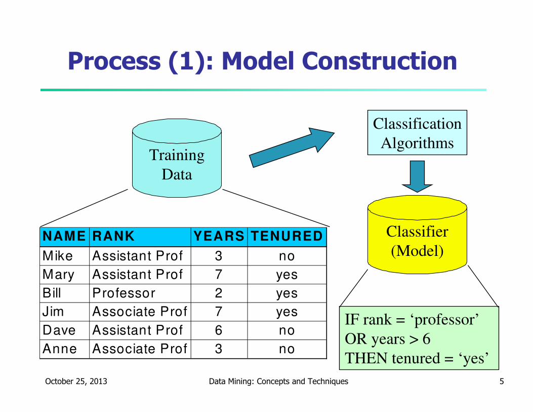
Classification—A Two-Step Process

� Model construction: describing a set of predetermined classes

� Each tuple/sample is assumed to belong to a predefined class, as determined by the class label attribute

� The set of tuples used for model construction is training set

� The model is represented as classification rules, decision trees, or mathematical formulae

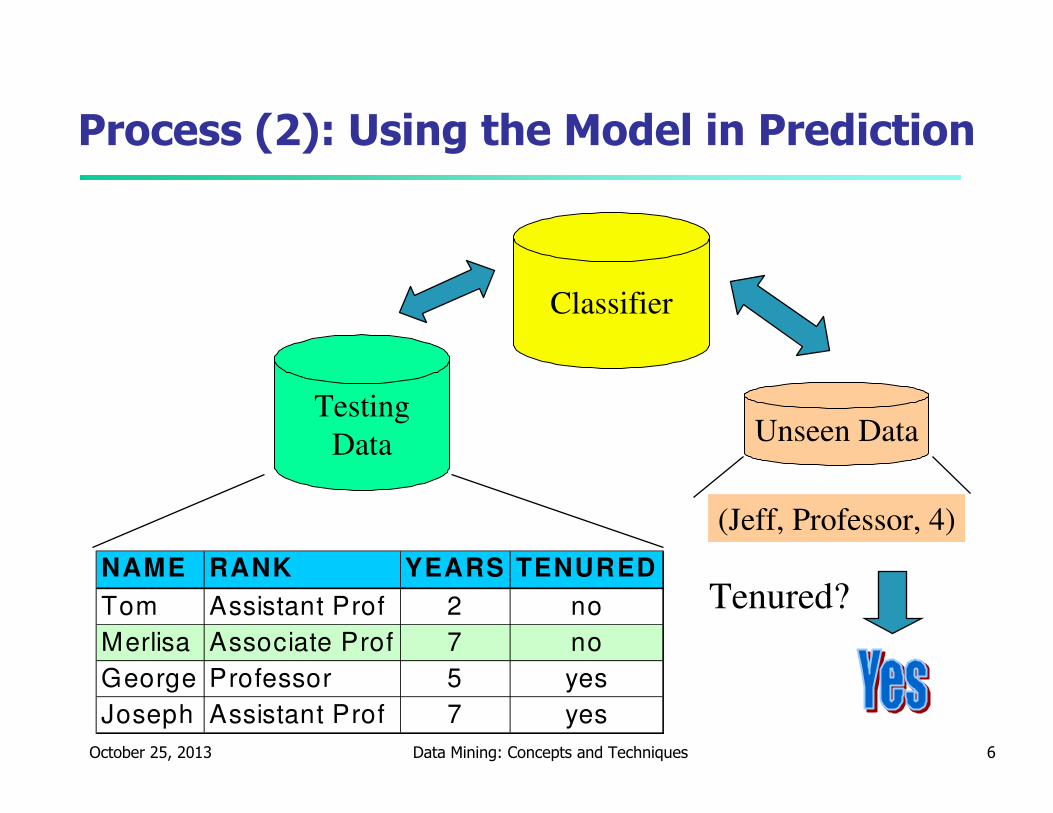
� Model usage: for classifying future or unknown objects

� Estimate accuracy of the model

� The known label of test sample is compared with the classified result from the model

� Accuracy rate is the percentage of test set samples that are correctly classified by the model

� Test set is independent of training set, otherwise over-fitting will occur

� If the accuracy is acceptable, use the model to classify datatuples whose class labels are not known


Process (1): Model Construction

Training

Data

NAME RANK YEARS TENURED

Mike Assistant Prof 3 no

Mary Assistant Prof 7 yes

Bill Professor 2 yes

Jim Associate Prof 7 yes

Dave Assistant Prof 6 no

Anne Associate Prof 3 no

Classification

Algorithms

IF rank = ‘professor’

OR years > 6

THEN tenured = ‘yes’

Classifier

(Model)


Process (2): Using the Model in Prediction

Classifier

Testing

Data

NAME RANK YEARS TENURED

Tom Assistant Prof 2 no

Merlisa Associate Prof 7 no

George Professor 5 yes

Joseph Assistant Prof 7 yes

Unseen Data

(Jeff, Professor, 4)

Tenured?


Issues: Data Preparation

� Data cleaning

� Preprocess data in order to reduce noise and handle

missing values

� Relevance analysis (feature selection)

� Remove the irrelevant or redundant attributes

� Data transformation

� Generalize and/or normalize data


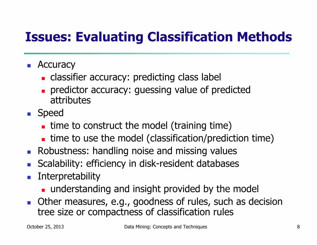
Issues: Evaluating Classification Methods

� Accuracy

� classifier accuracy: predicting class label

� predictor accuracy: guessing value of predicted attributes

� Speed

� time to construct the model (training time)

� time to use the model (classification/prediction time)

� Robustness: handling noise and missing values

� Scalability: efficiency in disk-resident databases

� Interpretability

� understanding and insight provided by the model

� Other measures, e.g., goodness of rules, such as decision tree size or compactness of classification rules


Decision Tree Induction: Training Dataset

age income student credit_rating buys_computer

<=30 high no fair no

<=30 high no excellent no

31…40 high no fair yes

>40 medium no fair yes

>40 low yes fair yes

>40 low yes excellent no

31…40 low yes excellent yes

<=30 medium no fair no

<=30 low yes fair yes

>40 medium yes fair yes

<=30 medium yes excellent yes

31…40 medium no excellent yes

31…40 high yes fair yes

>40 medium no excellent no

This follows an example of Quinlan’s ID3 (Playing Tennis)


Output: A Decision Tree for “buys_computer”

age?

overcast

student? credit rating?

<=30 >40

no yes yes

yes

31..40

no

fairexcellentyesno


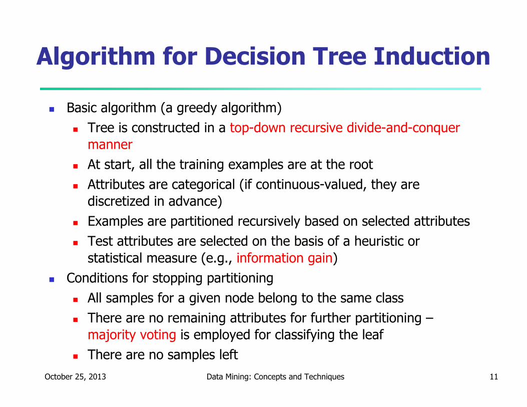
Algorithm for Decision Tree Induction

� Basic algorithm (a greedy algorithm)

� Tree is constructed in a top-down recursive divide-and-conquer

manner

� At start, all the training examples are at the root

� Attributes are categorical (if continuous-valued, they are

discretized in advance)

� Examples are partitioned recursively based on selected attributes

� Test attributes are selected on the basis of a heuristic or

statistical measure (e.g., information gain)

� Conditions for stopping partitioning

� All samples for a given node belong to the same class

� There are no remaining attributes for further partitioning –

majority voting is employed for classifying the leaf

� There are no samples left


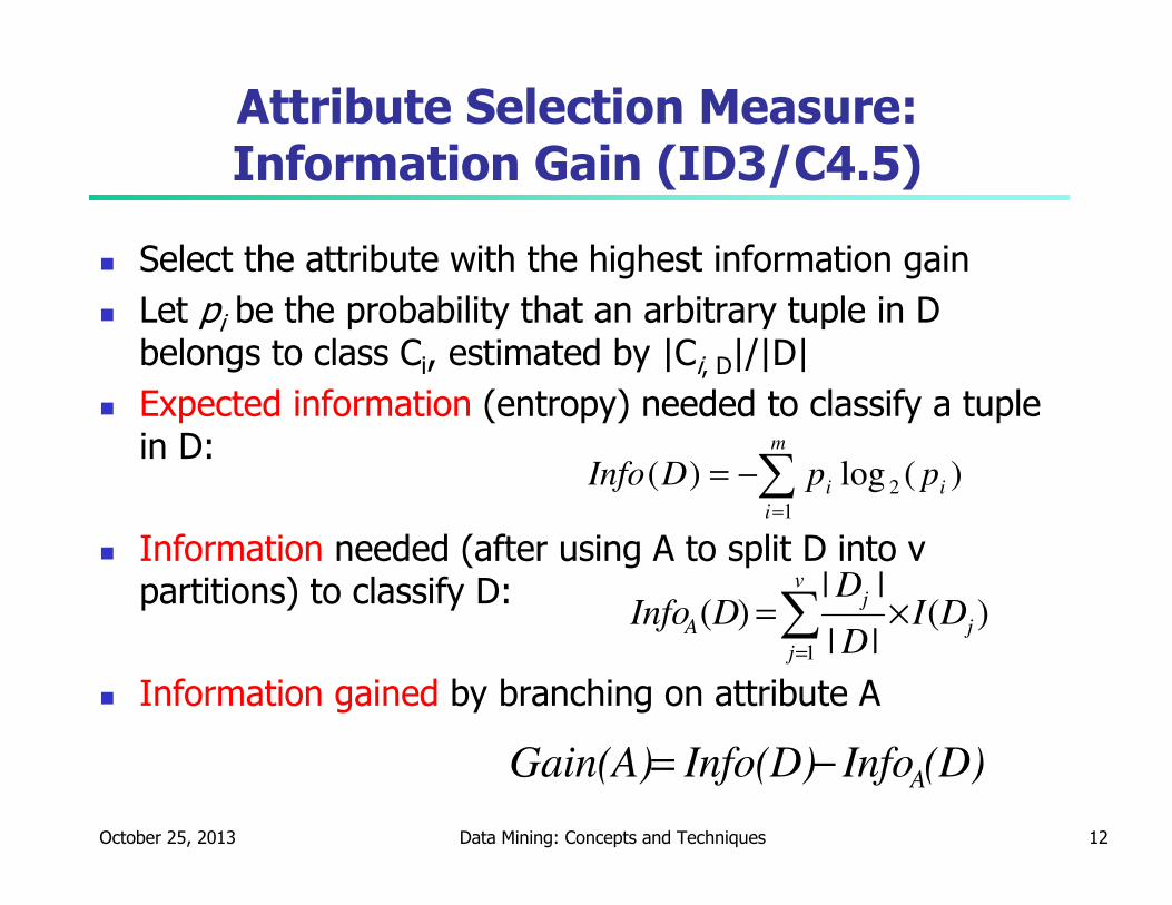
Attribute Selection Measure: Information Gain (ID3/C4.5)

� Select the attribute with the highest information gain

� Let pi be the probability that an arbitrary tuple in D belongs to class Ci, estimated by |Ci, D|/|D|

� Expected information (entropy) needed to classify a tuple in D:

� Information needed (after using A to split D into v partitions) to classify D:

� Information gained by branching on attribute A

)(log)( 2

1

i

m

i

i ppDInfo ∑=

−=

)(||

||)(

1

j

v

j

j

A DID

DDInfo ×=∑

=

(D)InfoInfo(D)Gain(A) A−=


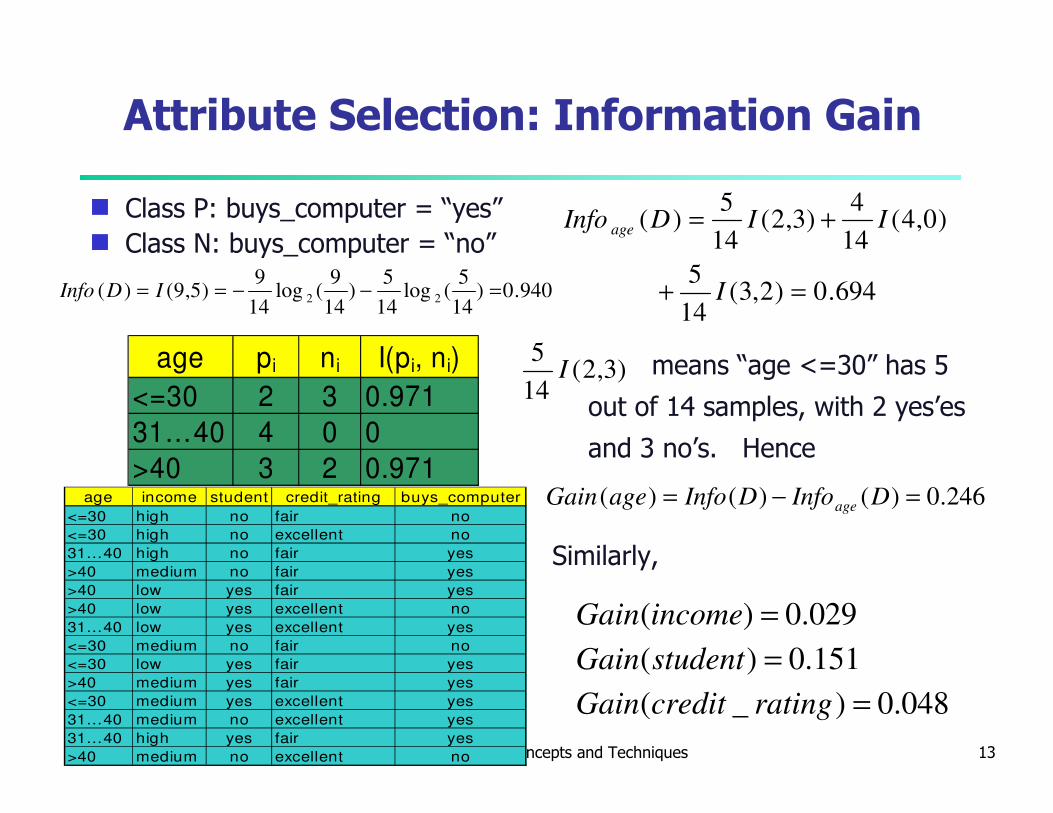
Attribute Selection: Information Gain

g Class P: buys_computer = “yes”

g Class N: buys_computer = “no”

means “age <=30” has 5

out of 14 samples, with 2 yes’es

and 3 no’s. Hence

Similarly,

age pi ni I(pi, ni)

<=30 2 3 0.971

31…40 4 0 0

>40 3 2 0.971

694.0)2,3(14

5

)0,4(14

4)3,2(

14

5)(

=+

+=

I

IIDInfo age

048.0)_(

151.0)(

029.0)(

=

=

=

ratingcreditGain

studentGain

incomeGain

246.0)()()( =−= DInfoDInfoageGain ageage income student credit_rating buys_computer

<=30 high no fair no

<=30 high no excellent no

31…40 high no fair yes

>40 medium no fair yes

>40 low yes fair yes

>40 low yes excellent no

31…40 low yes excellent yes

<=30 medium no fair no

<=30 low yes fair yes

>40 medium yes fair yes

<=30 medium yes excellent yes

31…40 medium no excellent yes

31…40 high yes fair yes

>40 medium no excellent no

)3,2(14

5I

940.0)14

5(log

14

5)

14

9(log

14

9)5,9()( 22 =−−== IDInfo


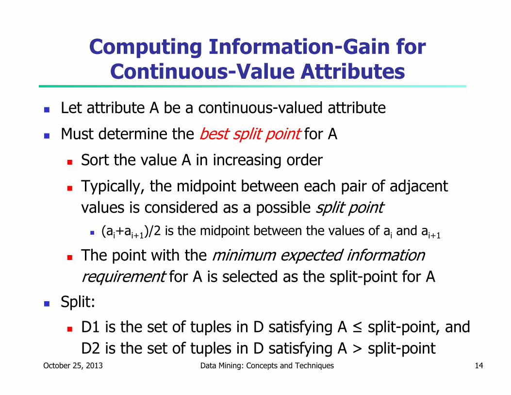
Computing Information-Gain for Continuous-Value Attributes

� Let attribute A be a continuous-valued attribute

� Must determine the best split point for A

� Sort the value A in increasing order

� Typically, the midpoint between each pair of adjacent

values is considered as a possible split point

� (ai+ai+1)/2 is the midpoint between the values of ai and ai+1

� The point with the minimum expected information

requirement for A is selected as the split-point for A

� Split:

� D1 is the set of tuples in D satisfying A ≤ split-point, and

D2 is the set of tuples in D satisfying A > split-point


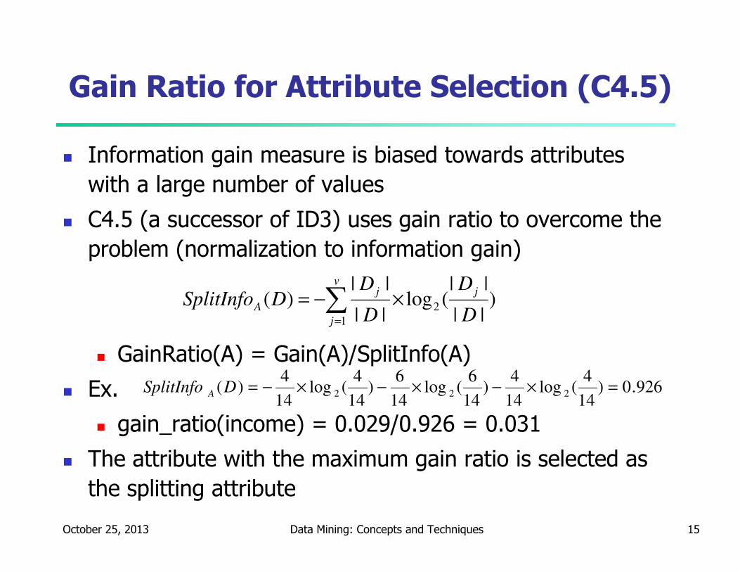
Gain Ratio for Attribute Selection (C4.5)

� Information gain measure is biased towards attributes

with a large number of values

� C4.5 (a successor of ID3) uses gain ratio to overcome the

problem (normalization to information gain)

� GainRatio(A) = Gain(A)/SplitInfo(A)

� Ex.

� gain_ratio(income) = 0.029/0.926 = 0.031

� The attribute with the maximum gain ratio is selected as

the splitting attribute

)||

||(log

||

||)( 2

1 D

D

D

DDSplitInfo

jv

j

j

A ×−= ∑=

926.0)14

4(log

14

4)

14

6(log

14

6)

14

4(log

14

4)( 222 =×−×−×−=DSplitInfo A


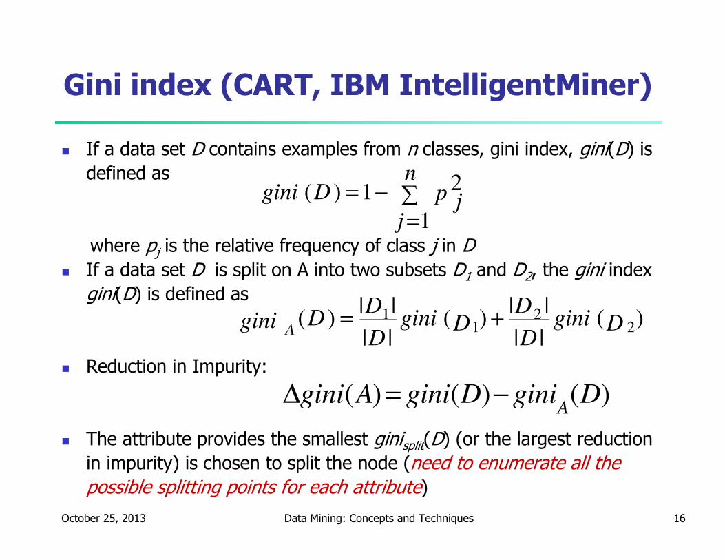
Gini index (CART, IBM IntelligentMiner)

� If a data set D contains examples from n classes, gini index, gini(D) is

defined as

where pj is the relative frequency of class j in D

� If a data set D is split on A into two subsets D1 and D2, the gini index

gini(D) is defined as

� Reduction in Impurity:

� The attribute provides the smallest ginisplit(D) (or the largest reduction

in impurity) is chosen to split the node (need to enumerate all the

possible splitting points for each attribute)

∑=

−=n

j

p jDgini

1

21)(

)(||

||)(

||

||)( 2

21

1Dgini

D

DDgini

D

DDgini A

+=

)()()( DginiDginiAginiA

−=∆


Gini index (CART, IBM IntelligentMiner)

� Ex. D has 9 tuples in buys_computer = “yes” and 5 in “no”

� Suppose the attribute income partitions D into 10 in D1: {low,

medium} and 4 in D2

but gini{medium,high} is 0.30 and thus the best since it is the lowest

� All attributes are assumed continuous-valued

� May need other tools, e.g., clustering, to get the possible split values

� Can be modified for categorical attributes

459.014

5

14

91)(

22

=

−

−=Dgini

)(14

4)(

14

10)( 11},{ DGiniDGiniDgini mediumlowincome

+

=∈


Comparing Attribute Selection Measures

� The three measures, in general, return good results but

� Information gain:

� biased towards multivalued attributes

� Gain ratio:

� tends to prefer unbalanced splits in which one

partition is much smaller than the others

� Gini index:

� biased to multivalued attributes

� has difficulty when # of classes is large

� tends to favor tests that result in equal-sized

partitions and purity in both partitions


Overfitting and Tree Pruning

� Overfitting: An induced tree may overfit the training data

� Too many branches, some may reflect anomalies due to noise or

outliers

� Poor accuracy for unseen samples

� Two approaches to avoid overfitting

� Prepruning: Halt tree construction early—do not split a node if this

would result in the goodness measure falling below a threshold

� Difficult to choose an appropriate threshold

� Postpruning: Remove branches from a “fully grown” tree—get a

sequence of progressively pruned trees

� Use a set of data different from the training data to decide

which is the “best pruned tree”


Classification in Large Databases

� Classification—a classical problem extensively studied by

statisticians and machine learning researchers

� Scalability: Classifying data sets with millions of examples

and hundreds of attributes with reasonable speed

� Why decision tree induction in data mining?

� relatively faster learning speed (than other classification methods)

� convertible to simple and easy to understand classification rules

� can use SQL queries for accessing databases

� comparable classification accuracy with other methods


Classification by Backpropagation

� Backpropagation: A neural network learning algorithm

� Started by psychologists and neurobiologists to develop

and test computational analogues of neurons

� A neural network: A set of connected input/output units

where each connection has a weight associated with it

� During the learning phase, the network learns by

adjusting the weights so as to be able to predict the

correct class label of the input tuples

� Also referred to as connectionist learning due to the

connections between units


Neural Network as a Classifier

� Weakness

� Long training time

� Require a number of parameters typically best determined empirically, e.g., the network topology or “structure.”

� Poor interpretability: Difficult to interpret the symbolic meaning behind the learned weights and of “hidden units” in the network

� Strength

� High tolerance to noisy data

� Ability to classify untrained patterns

� Well-suited for continuous-valued inputs and outputs

� Successful on a wide array of real-world data

� Algorithms are inherently parallel

� Techniques have recently been developed for the extraction of rules from trained neural networks


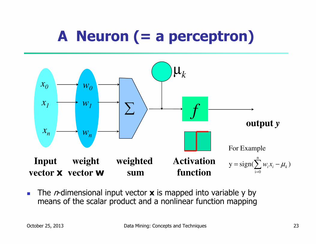
A Neuron (= a perceptron)

� The n-dimensional input vector x is mapped into variable y by means of the scalar product and a nonlinear function mapping

µk-

f

weighted

sum

Input

vector x

output y

Activation

function

weight

vector w

∑

w0

w1

wn

x0

x1

xn

)sign(y

ExampleFor

n

0i

kii xw µ−= ∑=


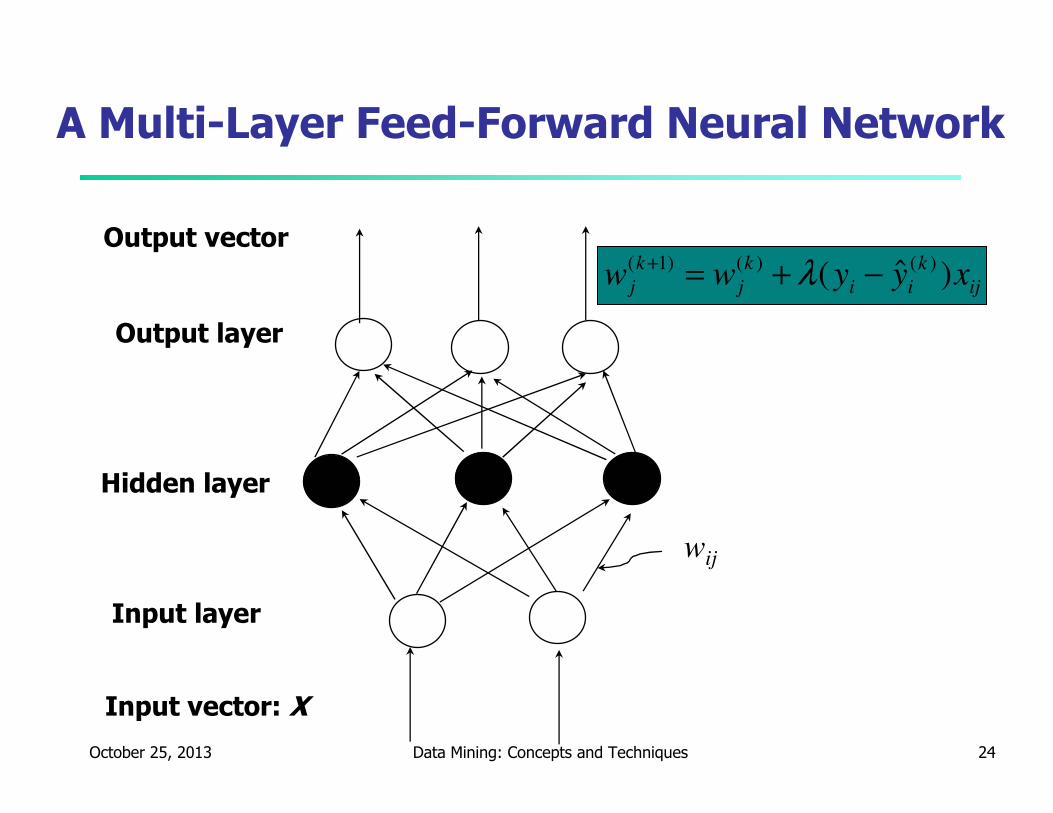
A Multi-Layer Feed-Forward Neural Network

Output layer

Input layer

Hidden layer

Output vector

Input vector: X

wij

ij

k

ii

k

j

k

j xyyww )ˆ( )()()1( −+=+ λ


How A Multi-Layer Neural Network Works?

� The inputs to the network correspond to the attributes measured

for each training tuple

� Inputs are fed simultaneously into the units making up the input

layer

� They are then weighted and fed simultaneously to a hidden layer

� The number of hidden layers is arbitrary, although usually only one

� The weighted outputs of the last hidden layer are input to units

making up the output layer, which emits the network's prediction

� The network is feed-forward in that none of the weights cycles

back to an input unit or to an output unit of a previous layer

� From a statistical point of view, networks perform nonlinear

regression: Given enough hidden units and enough training

samples, they can closely approximate any function


Defining a Network Topology

� First decide the network topology: # of units in the

input layer, # of hidden layers (if > 1), # of units in each

hidden layer, and # of units in the output layer

� Normalizing the input values for each attribute measured in

the training tuples to [0.0—1.0]

� One input unit per domain value, each initialized to 0

� Output, if for classification and more than two classes,

one output unit per class is used

� Once a network has been trained and its accuracy is

unacceptable, repeat the training process with a different

network topology or a different set of initial weights


Backpropagation

� Iteratively process a set of training tuples & compare the network's

prediction with the actual known target value

� For each training tuple, the weights are modified to minimize the

mean squared error between the network's prediction and the

actual target value

� Modifications are made in the “backwards” direction: from the output

layer, through each hidden layer down to the first hidden layer, hence

“backpropagation”

� Steps

� Initialize weights (to small random #s) and biases in the network

� Propagate the inputs forward (by applying activation function)

� Backpropagate the error (by updating weights and biases)

� Terminating condition (when error is very small, etc.)


Backpropagation and Interpretability

� Efficiency of backpropagation: Each epoch (one interation through the

training set) takes O(|D| * w), with |D| tuples and w weights, but # of

epochs can be exponential to n, the number of inputs, in the worst

case

� Rule extraction from networks: network pruning

� Simplify the network structure by removing weighted links that

have the least effect on the trained network

� Then perform link, unit, or activation value clustering

� The set of input and activation values are studied to derive rules

describing the relationship between the input and hidden unit

layers

� Sensitivity analysis: assess the impact that a given input variable has

on a network output. The knowledge gained from this analysis can be

represented in rules


Lazy vs. Eager Learning

� Lazy vs. eager learning

� Lazy learning (e.g., instance-based learning): Simply stores training data (or only minor processing) and waits until it is given a test tuple

� Eager learning (the above discussed methods): Given a set of training set, constructs a classification model before receiving new (e.g., test) data to classify

� Lazy: less time in training but more time in predicting

� Accuracy

� Lazy method effectively uses a richer hypothesis space since it uses many local linear functions to form its implicit global approximation to the target function

� Eager: must commit to a single hypothesis that covers the entire instance space


Lazy Learner: Instance-Based Methods

� Instance-based learning:

� Store training examples and delay the processing (“lazy evaluation”) until a new instance must be classified

� Typical approaches

� k-nearest neighbor approach

� Instances represented as points in a Euclidean space.

� Locally weighted regression

� Constructs local approximation

� Case-based reasoning

� Uses symbolic representations and knowledge-based inference


The k-Nearest Neighbor Algorithm

� All instances correspond to points in the n-D space

� The nearest neighbor are defined in terms of Euclidean distance, dist(X1, X2)

� Target function could be discrete- or real- valued

� For discrete-valued, k-NN returns the most common value among the k training examples nearest to xq

� Vonoroi diagram: the decision surface induced by 1-NN for a typical set of training examples

.

_+

_ xq

+

_ _+

_

_

+

.

..

. .


Discussion on the k-NN Algorithm

� k-NN for real-valued prediction for a given unknown tuple

� Returns the mean values of the k nearest neighbors

� Distance-weighted nearest neighbor algorithm

� Weight the contribution of each of the k neighbors

according to their distance to the query xq

� Give greater weight to closer neighbors

� Robust to noisy data by averaging k-nearest neighbors

� Curse of dimensionality: distance between neighbors could

be dominated by irrelevant attributes

� To overcome it, axes stretch or elimination of the least

relevant attributes

2),(

1

ixqxd

w≡


Genetic Algorithms (GA)

� Genetic Algorithm: based on an analogy to biological evolution

� An initial population is created consisting of randomly generated rules

� Each rule is represented by a string of bits

� E.g., if A1 and ¬A2 then C2 can be encoded as 100

� If an attribute has k > 2 values, k bits can be used

� Based on the notion of survival of the fittest, a new population is

formed to consist of the fittest rules and their offsprings

� The fitness of a rule is represented by its classification accuracy on a

set of training examples

� Offsprings are generated by crossover and mutation

� The process continues until a population P evolves when each rule in P

satisfies a prespecified threshold

� Slow but easily parallelizable


What Is Prediction?

� (Numerical) prediction is similar to classification

� construct a model

� use model to predict continuous or ordered value for a given input

� Prediction is different from classification

� Classification refers to predict categorical class label

� Prediction models continuous-valued functions

� Major method for prediction: regression

� model the relationship between one or more independent or predictor variables and a dependent or response variable

� Regression analysis

� Linear and multiple regression

� Non-linear regression

� Other regression methods: generalized linear model, Poisson regression, log-linear models, regression trees


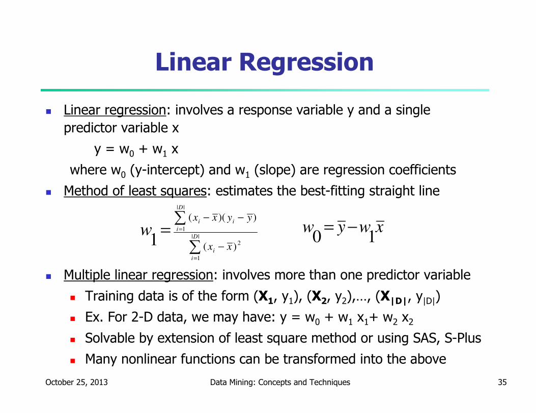
Linear Regression

� Linear regression: involves a response variable y and a single

predictor variable x

y = w0 + w1 x

where w0 (y-intercept) and w1 (slope) are regression coefficients

� Method of least squares: estimates the best-fitting straight line

� Multiple linear regression: involves more than one predictor variable

� Training data is of the form (X1, y1), (X2, y2),…, (X|D|, y|D|)

� Ex. For 2-D data, we may have: y = w0 + w1 x1+ w2 x2

� Solvable by extension of least square method or using SAS, S-Plus

� Many nonlinear functions can be transformed into the above

∑

∑

=

=

−

−−

=||

1

2

||

1

)(

))((

1 D

i

i

D

i

ii

xx

yyxx

w xwyw10

−=


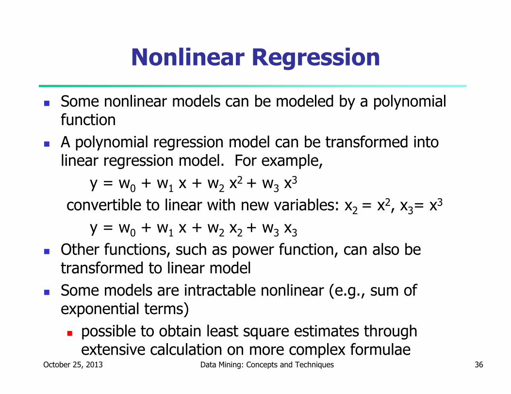
� Some nonlinear models can be modeled by a polynomial function

� A polynomial regression model can be transformed into linear regression model. For example,

y = w0 + w1 x + w2 x2 + w3 x3

convertible to linear with new variables: x2 = x2, x3= x3

y = w0 + w1 x + w2 x2 + w3 x3

� Other functions, such as power function, can also be transformed to linear model

� Some models are intractable nonlinear (e.g., sum of exponential terms)

� possible to obtain least square estimates through extensive calculation on more complex formulae

Nonlinear Regression


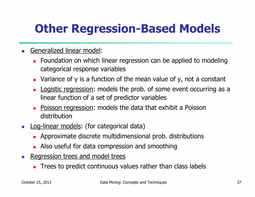
� Generalized linear model:

� Foundation on which linear regression can be applied to modeling

categorical response variables

� Variance of y is a function of the mean value of y, not a constant

� Logistic regression: models the prob. of some event occurring as a

linear function of a set of predictor variables

� Poisson regression: models the data that exhibit a Poisson

distribution

� Log-linear models: (for categorical data)

� Approximate discrete multidimensional prob. distributions

� Also useful for data compression and smoothing

� Regression trees and model trees

� Trees to predict continuous values rather than class labels

Other Regression-Based Models


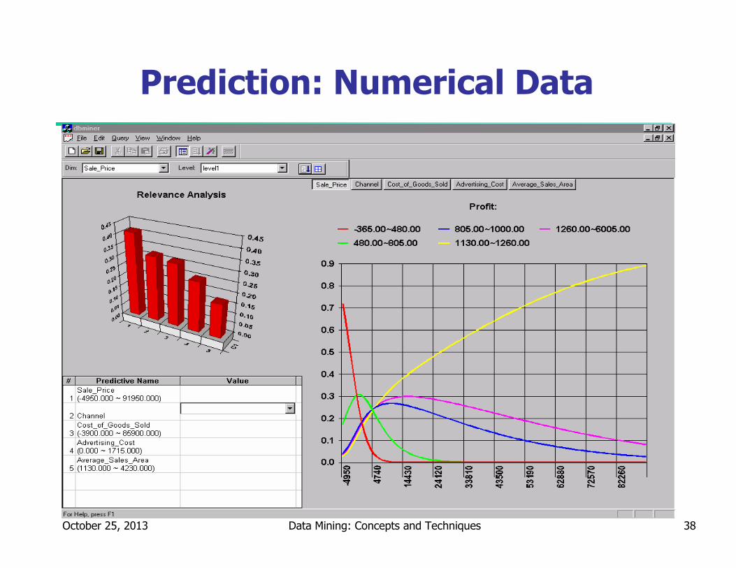
Prediction: Numerical Data


Prediction: Categorical Data


Classifier Accuracy Measures

� Accuracy of a classifier M, acc(M): percentage of test set tuples that are correctly classified by the model M

� Error rate (misclassification rate) of M = 1 – acc(M)

� Given m classes, CMi,j, an entry in a confusion matrix, indicates # of tuples in class i that are labeled by the classifier as class j

� Alternative accuracy measures (e.g., for cancer diagnosis)

sensitivity = t-pos/pos /* true positive recognition rate */

specificity = t-neg/neg /* true negative recognition rate */

precision = t-pos/(t-pos + f-pos)

accuracy = sensitivity * pos/(pos + neg) + specificity * neg/(pos + neg)

� This model can also be used for cost-benefit analysis

Real class\Predicted class buy_computer = yes buy_computer = no total recognition(%)

buy_computer = yes 6954 46 7000 99.34

buy_computer = no 412 2588 3000 86.27

total 7366 2634 10000 95.52

Real class\Predicted class C1 ~C1

C1 True positive False negative

~C1 False positive True negative


Predictor Error Measures

� Measure predictor accuracy: measure how far off the predicted value is

from the actual known value

� Loss function: measures the error betw. yi and the predicted value yi’

� Absolute error: | yi – yi’|

� Squared error: (yi – yi’)2

� Test error (generalization error): the average loss over the test set

� Mean absolute error: Mean squared error:

� Relative absolute error: Relative squared error:

The mean squared-error exaggerates the presence of outliers

Popularly use (square) root mean-square error, similarly, root relative

squared error

d

yyd

i

ii∑=

−1

|'|

d

yyd

i

ii∑=

−1

2)'(

∑

∑

=

=

−

−

d

i

i

d

i

ii

yy

yy

1

1

||

|'|

∑

∑

=

=

−

−

d

i

i

d

i

ii

yy

yy

1

2

1

2

)(

)'(


Evaluating the Accuracy of a Classifier or Predictor (I)

� Holdout method

� Given data is randomly partitioned into two independent sets

� Training set (e.g., 2/3) for model construction

� Test set (e.g., 1/3) for accuracy estimation

� Random sampling: a variation of holdout

� Repeat holdout k times, accuracy = avg. of the accuracies obtained

� Cross-validation (k-fold, where k = 10 is most popular)

� Randomly partition the data into k mutually exclusive subsets, each approximately equal size

� At i-th iteration, use Di as test set and others as training set

� Leave-one-out: k folds where k = # of tuples, for small sized data

� Stratified cross-validation: folds are stratified so that class dist. in each fold is approx. the same as that in the initial data


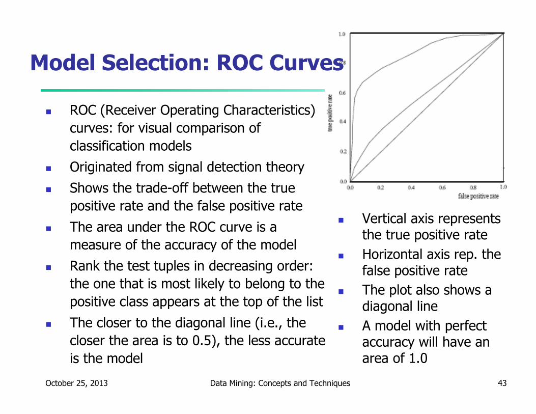
Model Selection: ROC Curves

� ROC (Receiver Operating Characteristics)

curves: for visual comparison of

classification models

� Originated from signal detection theory

� Shows the trade-off between the true

positive rate and the false positive rate

� The area under the ROC curve is a

measure of the accuracy of the model

� Rank the test tuples in decreasing order:

the one that is most likely to belong to the

positive class appears at the top of the list

� The closer to the diagonal line (i.e., the

closer the area is to 0.5), the less accurate

is the model

� Vertical axis represents the true positive rate

� Horizontal axis rep. the false positive rate

� The plot also shows a diagonal line

� A model with perfect accuracy will have an area of 1.0