


Languages
Pages
Legal

26
CHAPTER 4
KRISHNAGIRI RESERVOIR
4.1 PONNAIYAR RIVER
The River Ponnaiyar takes its source near Nandidurg in Karnataka
state South India at an altitude of 1000 m above MSL draining through
Southeastern slope of Chennakesava Hills. In Karnataka it is known as
‘Dhakshina Pinakini’. After traversing through the Devanahalli and Hoskote
taluks of Karnataka, it enters the Tamil Nadu state at a place near Bagalur
village of Hosur taluk. The River is called Ponnaiyar from this point in Tamil
Nadu.
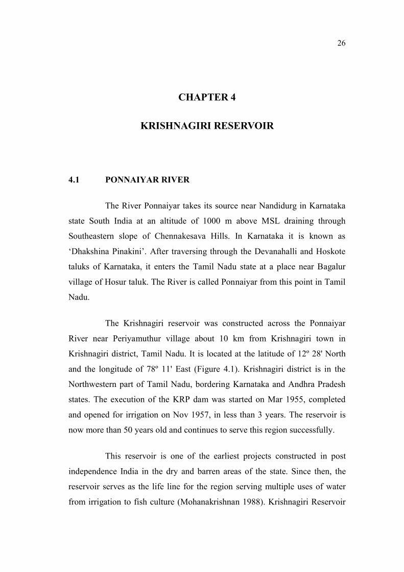
The Krishnagiri reservoir was constructed across the Ponnaiyar
River near Periyamuthur village about 10 km from Krishnagiri town in
Krishnagiri district, Tamil Nadu. It is located at the latitude of 12º 28' North
and the longitude of 78º 11' East (Figure 4.1). Krishnagiri district is in the
Northwestern part of Tamil Nadu, bordering Karnataka and Andhra Pradesh
states. The execution of the KRP dam was started on Mar 1955, completed
and opened for irrigation on Nov 1957, in less than 3 years. The reservoir is
now more than 50 years old and continues to serve this region successfully.
This reservoir is one of the earliest projects constructed in post
independence India in the dry and barren areas of the state. Since then, the
reservoir serves as the life line for the region serving multiple uses of water
from irrigation to fish culture (Mohanakrishnan 1988). Krishnagiri Reservoir

27
Figure 4.1 Krishnagiri Reservoir as Seen through Google Earth and Its location in Tamil Nadu, South India
TAMIL NADU

28
is a medium size storage and distribution structure with an initial capacity of
68.2×10⁶ m
3 and irrigates 3642 ha of wet crop area supplying water through
left and right main canals. The length of the Dam is 1000 m and at FRL, the
reservoir has a water spread area of 12.32 km2 and height of 22.8 m from the
river bed. The dam has 8 spillways, 3 river sluices and 2 canal sluices. The
hydraulic details are given in Table 4.1.
Table 4.1 Hydraulic Details of Krishnagiri Reservoir, Krishnagiri
District, Tamil Nadu
S. No. Description Detail
1 Full Reservoir Level Elevation 483.23m
2 Full Reservoir Level Capacity 68.2×10⁶
m3
3 Full Reservoir Level Watershed area 12.32 Km2
4 Maximum Water Level (Elevation) 484.75 m
5 Maximum Water Level (Capacity) 86.7×10⁶ m
3
6 Maximum Water Level (Waterspread area) 15.04 Km2
7 Height of the Dam 22.86 m
8 Length of the Dam 1.003 Km
9 Design Maximum Flood 4250.8 m3/s
10 River bed Level 464.63 m
11 Spillway 118.9×97.56 m
12 Spillway Capacity 4250 m3/s
There are 16 villages that directly benefit from this reservoir for
irrigation and other purposes. In addition, the LMC and RMC supply water to
the already existing tanks in these villages, where culture of fishes is also
taken up. There is water supply from the reservoir for a period of 10 months
in a year, and this ensures that culture operations completed successfully.

29
There are two spring channels that supply water to ayacut even
earlier to the construction of the reservoir, and the farmers have acquired
riparian rights and water supply is ensured for these original command areas
through spring channels throughout the year.
The LMC (Left Main Canal) take off near the spillway, while the
RMC (Right Main Canal) off take is on the western part of the water spread
on the earthen bund part of the Dam structure. During its span of half a
century of useful life, the reservoir encountered environmental problems in
later years (IHH 2007) probably due to industrial and agricultural
developments in the catchment area (Ravichandran and Kaarmegam 2004).
Several soil and water conservation programs have been implemented in the
catchment area of the reservoir by the Agricultural Engineering Department
and Forest Department of the Government of Tamil Nadu, since 1990’s. This
includes contour bunding, afforestation, bio fencing, construction of check
dams and percolation ponds.
4.2 ENVIRONMENTAL INVESTIGATIONS
Table 4.2 shows the reports available on different aspects of the
Krishnagiri Reservoir and its catchment area investigated by earlier workers
from the Centre for Water Resources, Anna University. An environmental
investigation in the study of the catchment area of the Krishnagiri Reservoir
(Ravichandran 2002) suggests that soil erosion and sediment bound nutrient
transport may be the main processes affecting the sedimentation and
eutrophication of the reservoir. Investigation of the soil erosion in the
catchment area using spatial data modeling in MapInfo environment
(Ravichandran and Kaarmegam 2004) indicated that some parts of the
watershed are having erodible soils and are contributing significant soil losses
from the catchment. In a UGC funded project (Ravichandran 2006), the
investigations in the reservoir was continued which mainly consisted of the
monitoring of water quality and the nutrient profiles systematically.

30
Table 4.2 Reports of Environmental Investigations Conducted in Krishnagiri Reservoir and its Catchment Area
Author Period of
study
Title of Report Feature Source
Ravichandran 2002 – 2003 A pilot study on nutrient export and
eutrophication of Krishnagiri Reservoir,
Krishnagiri, Tamil Nadu
Catchment erosion,
Water Quality study
Technical Report submitted to Institute for
Water Studies, PWD, Chennai 600 113
Karunakaran 2002 - 2004 Eutrophication of Krishnagiri Reservoir:
Causes and Environmental Impacts
USLE application, EIA,
Water quality of
Reservoir
Ph.D. thesis, Anna University, Chennai
600 025, 2005
Karunakaran
and
Ravichandran
2006 Estimation of Soil Erosion in
Krishnagiri Reservoir catchment of
Ponnaiyar basin in Tamil Nadu
Soil erosion and
impacts
Indian Journal of Soil Conservation 34(2):
110 – 113
Ravichandran
and Ramanibai
2005 – 2006 A hydrobiological and water quality
investigation in Krishnagiri Reservoir
Reservoir water quality,
algae
Technical Report, Anna University,
Chennai 600 025, 2006
Ravichandran, 2006 – 2008 Erosion based watershed modeling
approach for NPS pollution assessment
in Krishnagiri Reservoir catchment area
Catchment erosion
Hydrobiology
Reservoir water quality
Technical Report submitted to UGC, New
Delhi 110 002, 2008
Dhrissia 2007 – 2008 Studies on sedimentation in Krishnagiri
Reservoir
Sediment yield and
water quality
M E thesis, Anna University, Chennai 600
025, 2008
Ravichandran 2007 – 2008 Where have fishes gone? Reservoir water quality
fisheries and
community impacts
Illustrative cases for teaching IWRM,
Course manual published by SaciWaters,
Hyderabad, 2010

31
Karunakaran and Ravichandran (2006) in a study of 10 years of
data on rainfall in the catchment area have found that the rate as well as the
loss of total load of top soil from the catchment was influenced by total
rainfall received in a year and the number of severe storms during each of the
season. Two further studies, one on developing sediment graph for the
Krishnagiri Reservoir (Dhrissia 2008) and another study (Ravichandran 2010)
on the culture of fishes in the reservoir by the Fisheries Department of
Government of Tamil Nadu and the problems of decline in the yield faced
during the last decade in the reservoir were completed recently.
The Institute of Hydraulics and Hydrology at Poondi made an
investigation on the rate of sedimentation in the reservoir and estimated as
41.79% of loss of capacity as on 2006 (IHH 2007).
4.3 SECONDARY DATA
The hydrological data of the Krishnagiri Reservoir was provided by
the Water Resources Organisation of the Public Works Department of
Government of Tamil Nadu. The office of the Sub Divisional Officer,
Krishnagiri in the Krishnagiri Dam site collects daily data on water level,
inflow into the reservoir and regulate outflow through the irrigation supply
canals and river sluices. A fully functional automatic weather station is also
operated at the dam site by the Department. The basic climate data including
daily rainfall for the period March 2008 to June 2009 was collected from their
records and used in calculation of the weekly, monthly and seasonal profiles
of hydrological conditions of the reservoir. The water quality data was
collected as part of an environmental monitoring program in Krishnagiri
Reservoir Project being conducted since January 2008.
4.4 SAMPLING PROGRAM
A systematic collection of water samples was done at weekly
intervals from different locations in Krishnagiri Reservoir. Onsite

32
measurements for temperature, pH and Electrical Conductivity were done
using Eutech field meters and water samples are collected for analysis of
water chemistry and nutrients at the laboratory during Mar 2008 to Jun 2009
in the reservoir.
Water samples were collected from five locations in the reservoir
(Figure 4.2); location 1 is at Madhepatti village which is 500 m above the
water spread area in the Ponnaiyar River (Inflow), location 2 is near the boat
yard in the reservoir, location 3 is 100 m downstream of the head sluice of
LMC, location 4 is 100 m downstream of the head sluice of RMC and
location 5 is 200 m below the gates of spring channel. The first location
represents the inflows into the reservoir, the second location represents the
reservoir storage and the 3rd to 5th locations represent outflows from the
reservoir. Water samples were also collected from river sluice whenever
discharge took place during the period of study.
Figure 4.2 Krishnagiri Reservoir and the Sampling Locations for the
Study
33
The sampling program could not be conducted due to logistical
reasons during August 2008 and therefore no data is available for this period.
Similarly nitrates could not be analysed during March and April 2008 and no
data is available for this period also.
The pH and Electrical conductivity of the samples were measured
in the sampling location itself using portable meters (Eutech Inc). The
remaining parameters were analyzed in the laboratory of the Centre for Water
Resources at Chennai for the water samples collected in 1 liter clean
polythene containers and transported in an ice box. On most of the occasions
the samples were transported the same day and analysis started the next day.
4.5 ANALYTICAL METHODS
Standard Methods (APHA 2004) were followed for the estimation
of chemical parameters. Carbonates and bicarbonates were analysed by
titration in the unfiltered samples against standard acid and the alkalinity of
the sample was calculated. Chlorides were estimated by argentometric method
and total hardness was measured by EDTA complexometric method. The
nutrients Total Phosphate and Nitrate nitrogen were estimated by colorimetric
methods. The Ascorbic acid method was adopted for the estimation of
phosphates after digestion of the samples and the Cadmium reduction column
method was used for the analysis of nitrates.
Simple analytical tools in MS Excel were used for data preparations
and SPSS 10 was used for statistical analyses and preparation of graphical
illustrations.
4.6 RESERVOIR RELEASE AND TRAP EFFICIENCY
The sedimentation study took advantage of the earlier investigations
made in the Krishnagiri Reservoir and its catchment area. The rainfall,
inflows, sediment and other hydrological data for the period 1957 to 1985
34
except 1958 to 1965 was collected from a report on water resources
evaluation of Ponnaiyar basin by the Institute for Water Resources
Organisation PWD Government of Tamil Nadu (IWS, 1985) and for the
remaining period from the office of Water Resources Organisation in
Krishnagiri. The available hydrological data and other information is
compiled to test various models for Reservoir trap efficiency estimation and
compare their relative efficiency and utility in assessing the sediment
retention capacity of Krishnagiri Reservoir. The useful lifespan of the
reservoir and the possible environmental problems are also calculated and
discussed.
The sediment release efficiency of a reservoir is the mass ratio of
the released sediment (o
V ) to the total sediment inflow (i
V ) over a specified
time period. It is the complement of trap efficiency (TE):
100V
VVTE
i
oi ´-= (4.1)
Release efficiency = 100 – TE (4.2)
4.6.1 Brune Method
Brune (1953) developed an empirical relationship for estimating
long-term trap efficiency in normally impounded reservoirs based on the
correlation between the capacity to inflow ratio (C/I) and applied this method
to calculate trap efficiency observed in Tennessee Valley Authority reservoirs
in the southeastern United States. This is probably the most widely used
method for estimating the sediment retention in reservoirs, and gives
reasonable results from very limited data: storage volume and average annual
inflow. As a limitation, the method is applicable only to long-term average
conditions. Brune noted that significant departures can occur as a result of
changes in the operating rule. Brune has used the following equation:

35
)I
C(Log19.0970.0[TE = ]×100 (4.3)
Normally dry reservoirs tend to be less efficient at trapping
sediment, and shallow sediment-retention basins designed for the express
purpose of trapping sediment can operate much more efficiently than
indicated by the curve (Figure 4.3). For instance, the All-American Canal
desilting basins in Arizona would have negligible sediment trapping
efficiency based on their C/I ratio, but the basins operate at a trapping
efficiency of 91.7 percent. Trapping efficiency also depends on the actual
storage level at which the reservoir is held during flood periods (as opposed to
its nominal storage capacity), and the placement of outlets.
Figure 4.3 Trap Efficiency Related to C / I Inflow Ratio (Brune 1953)

36
4.6.2 Churchill Method
Churchill (1948) developed a relationship between the sediment
release efficiency and the sedimentation index of the reservoir, defined as the
ratio of the retention period to the mean flow velocity through the reservoir.
The minimum data required to use this method are storage volume, annual
inflow, and reservoir length. In applying the Churchill method, the following
definitions are used:
Capacity - Reservoir capacity at the mean operation
pool level for the analysis period (m3),
Inflow - Average daily inflow rate during study
period (m3/sec),
Retention period - Capacity divided by inflow rate (sec),
Length - Reservoir length at mean operating pool
level (m),
Velocity - Mean velocity computed by dividing inflow
by average cross-sectional area (m/sec).
The average cross-sectional area can be determined by dividing
reservoir capacity by length (m2).
Sedimentation index – Retention period divided by velocity
(sec2/m).
The sedimentation index computed form the above data is applied
to the curve (Figure 4.4) to estimate the sediment release efficiency.
Churchill’s method can be used to estimate the release efficiency in settling
basins, small reservoirs, flood retarding structures, semidry reservoirs, or
reservoirs that are continuously sluiced.

37
Figure 4.4 Churchill's (1948) Curves for Local and Upstream Sediment,
Relating TE to a Sedimentation Index
4.6.3 Brown Method
Brown (1944) developed a curve relating the ratio of reservoir
capacity (C, in acre-ft) and watershed area (W, in square miles) to trap
efficiency (TE in percent) and represented by the following equation:
]
)W
C(K1
11[100TE
´+-´= (4.4)
The coefficient K ranges from 0.046 to 1.0 with a median value of 0.1.
K increases:
(1) For regions of smaller and varied retention time (calculated
using the capacity-inflow ratio),

38
(2) As the average grain size increases, and
(3) For reservoir operations.
That prevents release of sediment through sluicing or movement of
sediment toward the outlets by pool elevation regulation. Variations are
mainly due to the fact that reservoirs having the same C/W ratio can have
different capacity inflow ratios. Brown’s curve is useful if the watershed area
and reservoir capacity is the only parameters known.
4.6.4 Gill Method
Later, Gill (1979) developed empirical equations which provided a
better fit to the three curves proposed by Brune.
Primarily for highly flocculated and coarse grained sediments:
25
2
)I
C(994701.0)
I
C(006297.0103.0
)I
C(
TE
++´=
- (4.5)
Median curve (for medium sediments) Morris and Wiggert (1972):
)I
C(02.1012.0
I
C
TE
+= (4.6)
Primarily for colloidal and dispersed fine-grained sediments:
3235
3
)I
C(02655.1)
I
C(02621.0)
I
C(10133.0101.0
)I
C(
TE
++´-´=
- (4.7)

39
4.7 PHOSPHATE DYNAMICS
4.7.1 Sources of Data
Table 4.2 shows the investigations conducted in the Krishnagiri
Reservoir project area since 2001 by different authors from the CWR, Anna
University and University of Madras, both at Chennai. Information on water
quality including phosphate concentration in the reservoir has been part of
these investigations starting with the initial study on the nutrient load from the
watershed in 2002.
During the course of collection of data, only monthly values are
collected. The gaps in data especially during 2005 and 2007 with missing
values especially for inflow and outflow concentrations were noticed. The
missing data was estimated by the linear interpolation method and the data
series for each year was then completed. However, there were no gaps in
hydrological data for the above period and the daily values are converted into
monthly averages for further analysis.
4.7.2 Data Analysis
The data analysis was done in MS Excel spreadsheet to prepare
graphical illustrations. Figure 4.5 shows the general classification and
grouping of data, before the computation and estimation of the parameters
was done.
Initially all the data were listed as monthly values from January
2001 to June 2009. However, when calculating the annual loads, the calendar
year may not be appropriate, as the seasonal climatic conditions are different
in this part of the sub tropical region. The water year starts with the onset of

40
the southwest monsoon season in June that lasts for four months and followed
by the north east monsoon for another three months from October to December.
Figure 4.5 Analysis Scheme Adopted in the Study for Hydrological and
Water Quality Data
The winter is brief (Jan - Feb) and then the summer follows (March
to May). Therefore, the water year can be divided into monsoon (Jun - Dec)
and post monsoon (Jan - May) seasons. Therefore, the water year was
considered as more rational to study and compare the effects and all the data
were grouped into four seasons (Figure 4.5) before further analysis.
4.7.3 Hydrological Analysis
The hydrological changes in the reservoir from 2001 to 2009 were
assessed on the basis of daily water level, inflow, and discharge and rainfall
data as monthly averages. The methods employed for the computation and
input data are explained below. This include total inflow, total outflow,
reservoir volume, surface area, evaporation, rainfall inflow, mean depth,
hydraulic flushing rate and the hydraulic residence time.
Data calendar (Jan – Dec)
Water year (Jun – May)
Monsoon (Jun – Dec) Post Monsoon (Jan – May)
SWM (Jun – Sep) NEM (Oct – Dec) WIN (Jan – Feb) SUM (Mar – May)
41
The total inflow and total outflow was computed by the summation
of the daily values of inflow and outflow data for the reservoir. The inflows
include discharge from the Ponnaiyar River and inflows due to rainfall over
the reservoir. The outflow includes the discharge through the left and right
main canals, the river sluices and the spring channel excluding evaporation
losses.
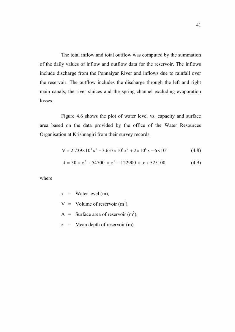
Figure 4.6 shows the plot of water level vs. capacity and surface
area based on the data provided by the office of the Water Resources
Organisation at Krishnagiri from their survey records.
662534106x102x10637.3x10739.2V ´-´+´-´= (4.8)
525100122900547003023 +´-´+´= xxxA (4.9)
where
x = Water level (m),
V = Volume of reservoir (m3),
A = Surface area of reservoir (m2),
z = Mean depth of reservoir (m).

42
Figure 4.6 Water Level vs. Capacity and Surface Area Relations in
Krishnagiri Reservoir
The reservoir volume and surface area were calculated based on the
changes in daily water levels by reference to the Figure 4.6.
4.7.4 Hydraulic Budget
The hydraulic budget was calculated for the reservoir based on the
hydrological data available.
Cap
acit
y (
x1
06m
3)
43
The hydraulic Flushing Rate (HFR) is the number of times a
volume of water equal to the volume of the reservoir flows through the
reservoir per that time. It was calculated by
V
Qout=r (4.10)
where
ρ = Hydraulic flushing rate (yr-1
),
outQ = Total hydraulic outflow (m
3/yr),
V = Volume of reservoir (m3).
The Hydraulic Residence Time (HRT) of a reservoir is the average
amount of time that water remains in the reservoir. It is the inverse of the
HFR and is computed as follows:
outQ
V=t (4.11)
r=t1
(4.12)
where is residence time of water in reservoir.
Areal Hydraulic Loading Rate was calculated as follows:
A
Qq 1
s = (4.13)
where
1Q = Hydraulic inflow rate (m
3/yr),
A = Surface area of the reservoir (m2),
44
sq = Areal hydraulic loading rate (m/yr).
The Apparent Settling Velocity (ASV) was computed according to
Reckhow (1979), as follows:
sq2.06.11v ´+= (4.14)
where
v = Apparent settling velocity (m/sec).
The response time of the reservoir is computed as follows and it
represents a measure of the time it would take for the reservoir to respond to a
change in its phosphorus loading. Response time is a function of the
reservoir’s flushing rate and is independent of either the reservoir’s
phosphorus load or content. Because the rate at which a substance is
accumulated or removed from a lake is a logarithmic function, response time
is usually expressed as the time it would take to increase or reduce the
concentration of a substance by one-half and can be estimated by the
following equation (Dillon and Rigler 1975):
z
10HFR
69.0)2/1(RT
+= (4.15)
where
HFR = Hydraulic flushing rate of reservoir (yr-1
),
z = Mean depth of reservoir (m).
4.7.5 Phosphate Profile
The Total Phosphate concentration profile of the reservoir during
the period of 9 years (2001-2009) was collected from several authors

45
(Table 4.2) and averaged for monthly values, and used in calculations. This
include Total phosphate concentration measured at a point above the water
spread area in the Ponnaiyar River (TPin), within the water spread area, mostly
near the boat yard (TPres) and in the outflow channels and/or river sluice
(TPout).
4.7.6 Phosphate Load
The total phosphate load was computed by multiplying the monthly
inflow and outflow values by respective average phosphate concentration data
for each month. The reservoir phosphate load was computed by multiplying
the average lake volume by total phosphate concentration measured in the
reservoir.
The areal phosphate loading rate (L) was computed by dividing the
monthly total phosphate input load by the average surface area of the
reservoir during this period.
A
ML = (4.16)
where
M = Total phosphate input load to reservoir (mg/yr),
L = Areal phosphate loading rate (mg/yr/m2),
A = surface area of reservoir (m2).
46
4.8 PHOSPHORUS RETENTION COEFFICIENT (R) AND
SEDIMENTATION COEFFICIENTS (σ)
The P retention and the sedimentation coefficient for the study
period were calculated by different method available in literature. The
Table 4.3 lists the authors, and the method of calculation of the retention
coefficients. Eight methods of calculating the phosphate retention (R) and 5
methods of sedimentation coefficient ( ) were calculated for the data
available. All these methods have been used in the mass balance model for
estimating the TPres concentration as follows (Brett and Benjamin 2008).
t´s´+´=b1
TPaTP in
res (4.17)
a is the coefficient representing constant loss of TP and b is the
coefficient representing first order rate constant for TP loss due to various
processes. The sedimentation coefficient ( ) is the key parameter in the mass
balance modelling and its prediction is important in the success of the model.
The relationship between the sigma and the input - output load of phosphate
was plotted to analyse the relationship during different seasons of the year
with the available data. Table 4.4 shows the different methods used for the
computation of sedimentation coefficient.
The evaluation of the different methods of computing R and was
done separately for different seasons, monsoon and post monsoon seasons by
two criteria; a table of RMS error and a plot of predicted vs. observed value of
TP concentration. The methods that produced less error and showed better fit
of data with the Krishnagiri Reservoir are used for further computation and
presentation.

47
Table 4.3 Mass Balance Models Applied for Prediction of Phosphate
Retention Coefficient (R) in Krishnagiri Reservoir
S. No. Author Formula
1 Chapra (1975)sqv
vR +=
2 Larsen and Mercier (1976)r+=
1
1R
551.0515.01
1R r´+=
3 Kirchner and Dillon (1975) ss q00949.0q271.0e574.0e426.0R-- ´+´=
4 Nurenberg (1984)sq18
15R +=
5 Prairie (1989) t´+t´+=
18.01
18.025.0R
6 Hejzlar et al (2006)t´+
t´=84.11
84.1R
88.0in
in
)1
P(
P
43.11R t+-=
Table 4.4 Sedimentation Models Applied for Prediction of TP in
Krishnagiri Reservoir
S.No. Author Formula Explanation
1 Vollenweider (1975)z
10=s2 Welch et al. (1986)
78.0r=s3
Larsen and Mercier (1976) 49.083.0 -t´=s4 472.0761.0 -t´=s5
Michael T. Brett and
Mark M. Benjamin ( 2008))R1(
R
-´t=s
R from Chapra (1975)
6R from Larsen and Mercier
(1976-a)
7 R from Larsen and Mercier (1976-b)
8 R from Kirchner and Dillon (1975)
9 R from Nurnberg (1984)
10 R from Prairie (1989)
11R from Hejzlar et al (2006)
1 for Reservoirs
2 for Reservoirs and Lakes12
48
4.9 PRESENT STUDY
The application of different methods of P retention and
sedimentation to Krishnagiri Reservoir data provided opportunity to explore,
analyse and propose a method for computing Pin (calculated) concentration,
by modifying the model proposed by Canfield and Bachmann (1981). This
method provided a better fit of the data for Krishnagiri Reservoir and is
described in chapter 7.
Top Related