


Languages
Pages
Legal

15
CHAPTER 3
MINIMUM SPANNING TREE BASED
CLUSTERING ALGORITHMS
3.1 Introduction
In this chapter, we present two clustering algorithms based on the minimum spanning
tree. The first algorithm is designed using coefficient of variation. The second
clustering algorithm is developed based on the dynamic validity index. Both the
algorithms are experimented on various synthetic as well as biological data and the
results are compared with some existing clustering algorithms using dynamic validity
index and runtime.
3.2 Terminologies
We first describe some terminologies which are useful to understand the proposed
algorithms as follows.
3.2.1 Minimum Spanning Tree
Minimum Spanning Tree (MST) [148] is a sub-graph that spans over all the vertices
of a given graph without any cycle and has minimum sum of weights over all the
included edges. In MST-based clustering, the weight for each edge is considered as
the Euclidean distance between the end points forming that edge. As a result, any
edge that connects two sub-trees in the MST must be the shortest. In such clustering
methods, inconsistent edges which are unusually longer are removed from the MST.
The connected components of the MST obtained by removing these edges are treated
as the clusters. Elimination of the longest edge results into two-group clustering.
Removal of the next longest edge results into three-group clustering and so on [27].
16
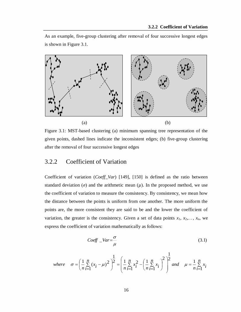
As an example, five-group clustering after removal of four successive longest edges
is shown in Figure 3.1.
(a) (b)
Figure 3.1: MST-based clustering (a) minimum spanning tree representation of the
given points, dashed lines indicate the inconsistent edges; (b) five-group clustering
after the removal of four successive longest edges
3.2.2 Coefficient of Variation
Coefficient of variation (Coeff_Var) [149], [150] is defined as the ratio between
standard deviation (σ) and the arithmetic mean (µ). In the proposed method, we use
the coefficient of variation to measure the consistency. By consistency, we mean how
the distance between the points is uniform from one another. The more uniform the
points are, the more consistent they are said to be and the lower the coefficient of
variation, the greater is the consistency. Given a set of data points x1, x2,, xn, we
express the coefficient of variation mathematically as follows:
)1.3(_
VarCoeff
n
iix
nand
n
iix
n
n
iix
n
n
iix
nwhere
1
121
2
1
1
1
2121
1
2)(1
3.2.2 Coefficient of Variation
17
We use a threshold value on the coefficient of variation (Coeff_Var) to
determine the inconsistent edges for their removal from the minimum spanning tree
of the given data set in order to produce the clusters.
3.2.3 Dynamic Validity Index
A validity index is used to evaluate the quality of the clusters produced by the
clustering algorithm. Several validity indices have been proposed in the literature.
However, most of them are suitable for well separated data. The clusters of the
complex data sets can be of arbitrary shapes and sizes. We may not always encounter
with well-separated clusters. Hence, it is highly essential to use an efficient validity
measure of clustering, especially in the case of genome data. For performance
measure of the proposed algorithm, we use here dynamic validity index (DVI) [151]
defined as follows. Let n be the number of data points, k be the pre-defined upper
bound of the number of clusters, and zi be the center of the cluster Ci. The dynamic
validity index is given by
)2.3()}(*)({,,2,1
min pInterRatiopIntraRatiokp
DVI
where the IntraRatio and InterRatio are defined as follows.
)3.3()(
)(,)(
)(MaxInter
pInterpInterRatio
MaxIntra
pIntrapIntraRatio
)4.3())((,...,2,1
max,1
21)( iIntra
kiMaxIntra
p
i iCxizx
npIntra
)5.3(1
1
2
1
2
2
,
)(
p
i p
jjziz
jzizjiMin
jzizjiMax
pInter
3.2.3 Dynamic Validity Index

18
and )6.3())((.,...,2,1
max iInterki
MaxInter
Here, Intra Ratio stands for the overall compactness of clusters scaled from
Intra term, where as Inter Ratio represents overall separation of clusters scaled from
Inter term. The Intra term is the average distance of all the points within a cluster
from cluster center. Then we have Inter term which is composed of two parts, both of
them based on cluster centers. The value of Inter increases with the increment in k.
The symbol in the equation of DVI represents the modulating parameter to balance
the noisy data points. If there is no noise in the data the value of is set to 1.
3.3 Proposed Algorithms
We present the proposed algorithms in separate subsections as follows.
3.3.1 Algorithm Based on Coefficient of Variation
We first provided an outline of the proposed method as follows. The algorithm
comprises of two basic procedures namely, the main and the core. In the main, we
find the minimum spanning tree of the given data. Next, we sort the edges of the
MST in non-decreasing order of the weights and store them in Edgelist. Then the
procedure core is applied on this sorted edge list. We also run the core on the same
list but in the reverse order. The edges are added or removed in the process of cluster
formation depending on some criterion over the threshold value. Then we update the
edge list and run the core algorithm on the updated list. This process is repeated until
there is no change in the edge list.
In the procedure core, we input a sorted array of the MST edges of the given
data points. We pick up one edge at a time from this sorted array and calculate the
coefficient of variation. If the coefficient of variation is less than the given threshold
value, then that edge is added to the EdgeSel or EdgeRej (defined later). This process
is repeated until an edge is detected for which the coefficient of variation is greater
3.3 Proposed Algorithms

19
than the threshold value.
The intuitive idea behind the core algorithm is that it groups the similar edges
having approximately equal weights. Here, the weight of an edge is the Euclidean
distance between the terminal points of the edges. It judges the edge by assuming its
inclusion in the cluster structure. Then it calculates the coefficient of variation of all
the included edges along with the present edge. If the coefficient of variation exceeds
the given threshold value, it discards the remaining edges along with the current edge
and this edge is treated as an inconsistent edge with respect to the edges added to the
group. Otherwise, the edge is added to the group and then the next edge is taken for
the consideration. This is continued till the encounter of inconsistent edge or end of
the list. The group of edges is the Edgelist which is initialized to NULL. An edge is
added to the group by adding it to the list. If the edges are selected from the edge list
sorted in non-decreasing order of their weights, then these edges are meant for
selection in the final cluster. However, if the list is sorted in non-increasing order,
these edges are meant for the rejection.
In the proposed algorithm, there is no need to input any prior information such
as cluster numbers, limit on cluster size or initial configuration. It tries to find the
optimal cluster number and configuration. We now formally present our algorithm
step wise as follows.
3.3.1 Algorithm Based on Coefficient of Variation

20
Algorithm MST-CV (Threshold)
Notations used in the algorithm:
(Pat)n×d: Pattern matrix of n data elements having d dimensions. Pat(i, j) gives the
value of the ith data point of j
th dimension.
(Prox)n×n: Proximity matrix of n2 elements holding Euclidean distance between two
points of the given data set. The Pattern matrix is converted into Proximity
matrix. Prox(l, m) is the Euclidean distance between the lth
and mth
data
points. Note that Prox(i, j) = Prox(j, i) and Prox(i, i) = 0.
(Output)n×n: Output matrix holding the clustering result. It is basically an adjacency
matrix consisting of various components (clusters) in the graph.
Weight(e): Euclidean distance between the end points of the edge ‘e’.
Edgelist: It is a list that holds the edges obtained by the MST algorithm (Prim’s
algorithm) along with their Euclidean distance.
Start(Edgelist): It is the index of the 1st element of Edgelist
EdgeSel: It holds the edges selected by the core algorithm. The edges in this list
actually form the clusters.
Length(EdgeSel): It is the cardinality of EdgeSel.
EdgeRej: It contains the edges rejected by the core algorithm.
Threshold: A given limit of the coefficient of variation.
The Main Algorithm:
Input: The pattern matrix (Pat)n×d
Output: The Output matrix (Output)n×n
Pre-processing: Convert pattern matrix (Pat)n×d to proximity matrix (Prox)n×n by the
following formula:
2)),(),((),( kjPatkiPatjiprox for 1 ≤ k ≤ d.

21
Step 1: Run Prim’s algorithm on Prox and store the edges of the MST in Edgelist.
Step 2: Sort the Edgelist into non-decreasing order of their weights.
Step 3: Run the core Algorithm on Edgelist to store the result into EdgeSel.
Step 4: Run the core Algorithm on the reversed Edgelist (i.e., non-increasing) to
store the result into EdgeRej.
Step 5: If EdgeSel and EdgeRej have no edge in common, then remove all the edges
from Edgelist that belong to EdgeRej; otherwise remove the largest edge
from EdgeSel .
Step 6: Add all the edges belonging to EdgeSel to the Output matrix.
Step 7: Update Edgelist by removing the 1st half of the edges of the EdgeSel from the
Edgelist,
)](2/)([.. EdgelistStartEdgeSelLengthEdgelistEdgelistei
Step 8: Run the core Algorithm on the updated Edgelist.
Step 9: Repeat the steps 6 to 8 until there is a change in the EdgeSel.
□
The Core Algorithm:
Input: Edgelist
Output: EdgeSel, EdgeRej
Step 1: Sum1, Count, Sum2 0
EdgeSel, EdgeRej NULL
Step 2: For each edge ‘e’ in Edgelist do
/* Calculation of the Coefficient of Variation */
{
Sum1 Sum1 + Weight(e)
Sum2 Sum2 + (Weight(e))2
Count Count + 1
Mean Sum1 / Count
2/1
)2
)/2(( MeantCounSumSD
3.3.1 Algorithm Based on Coefficient of Variation
22
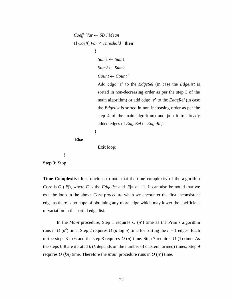
Coeff_Var SD / Mean
If Coeff_Var < Threshold then
{
Sum1 Sum1
Sum2 Sum2
Count Count
Add edge ‘e’ to the EdgeSel (in case the Edgelist is
sorted in non-decreasing order as per the step 3 of the
main algorithm) or add edge ‘e’ to the EdgeRej (in case
the Edgelist is sorted in non-increasing order as per the
step 4 of the main algorithm) and join it to already
added edges of EdgeSel or EdgeRej.
}
Else
Exit loop;
}
Step 3: Stop
Time Complexity: It is obvious to note that the time complexity of the algorithm
Core is O (|E|), where E is the Edgelist and |E|= n 1. It can also be noted that we
exit the loop in the above Core procedure when we encounter the first inconsistent
edge as there is no hope of obtaining any more edge which may lower the coefficient
of variation in the sorted edge list.
In the Main procedure, Step 1 requires O (n2) time as the Prim’s algorithm
runs in O (n2) time. Step 2 requires O (n log n) time for sorting the n 1 edges. Each
of the steps 3 to 6 and the step 8 requires O (n) time. Step 7 requires O (1) time. As
the steps 6-8 are iterated k (k depends on the number of clusters formed) times, Step 9
requires O (kn) time. Therefore the Main procedure runs in O (n2) time.
23
3.3.2 Experimental Results
For the visualization purpose, we initially tested the proposed algorithm on various
benchmark synthetic data sets which are complex for clustering. We also run the
algorithm on various benchmark gene expression data [32], [33]. The experiments
were performed using MATLAB on an Intel Core 2 Duo Processor machine with
T9400 chipset, 2.53 GHz CPU and 2 GB RAM running on Microsoft Windows Vista.
We used the same experimental setup for all the proposed algorithms throughout this
thesis. We compared the proposed algorithm with the classical K-means [26], SFMST
[59], SC [152], MSDR [58], IMST [49], SAM [64] and MinClue [60]. In case of
multi-dimensional gene expression data we used dynamic validity index DVI
(defined in section 3.2.3) as a measure of the quality of clusters. The proposed
method detected the outliers in the form of separate clusters with significantly small
number of points compared to the actual clusters. Hence, the clusters with
considerably small size are declared as outliers by using a limit on the cardinality of
all the clusters. An important issue involved in the proposed algorithm is the proper
selection of the threshold value for the coefficient of variation. This can range from 0
to 1. The smaller the threshold, the larger is the number of edges to be eliminated and
in that case it produces a large number of clusters. The larger the threshold value, the
more is the number of edges to be added to the cluster and even inconsistent edges
become the part of the clusters. The algorithm is tested varying the threshold value
from 0.1 to 0.9. It is observed that the optimal results are obtained for threshold value
within the range 0.2 to 0.6 inclusive of both. The results are as follows.
3.3.3 Synthetic Data
We consider here a few generated artificial data sets namely, two-band, cluster inside
cluster, three-group, two-moon crescent, density-separated and swirl data. These data
sets are usually known to be complex for clustering. The data sets are described as
follows.
3.3.2 Experimental Results
24
Two-band data: The objects of this data set are grouped in the form of two bands,
where each band represents a cluster. Here, the size of each cluster/band is 200. Few
points are plotted little far away from the two bands to represent the outliers.
Cluster-inside-cluster data: This is a special type of data set, where all the objects
of one cluster lie inside another cluster. The total number of objects of this data set is
693 and distributed to two clusters. To examine the outlier detection capability, we
have also given a few points as outliers.
Three-group data: There are three clusters in this data set and its total size is 300.
Unlike the above mentioned data sets, here the points of the clusters are not of
uniform shaped. Few outliers are also involved around all the 3 clusters.
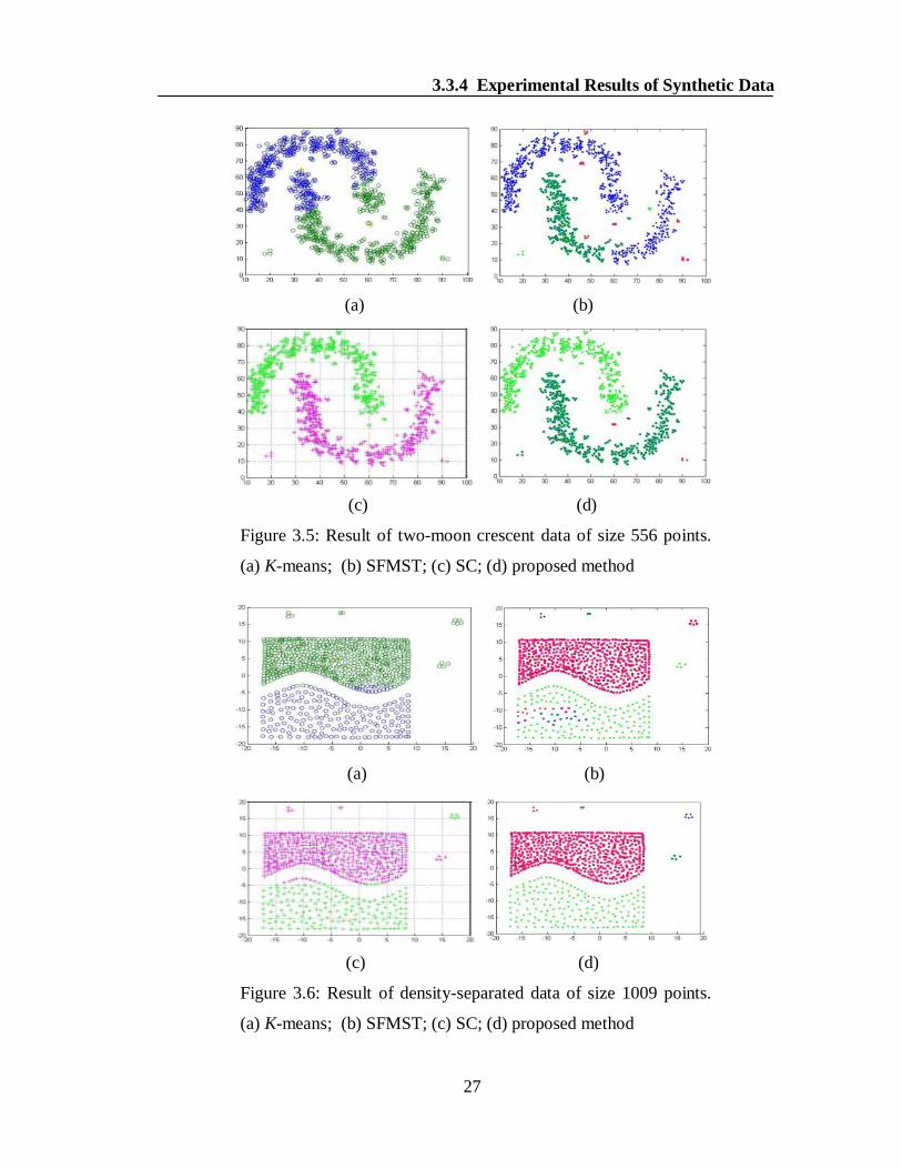
Two-moon crescent data: This data set represents two clusters which are of crescent
moon shaped. Here few points are also given as outliers to represent the stars.
Simply, the clusters of this data set represent the moons and outliers represent the
stars. The size of this data set is 556.
Density-separated data: The clusters in this data set are separated by the density.
Number of clusters of this data is two and the cardinality is 1009. Like the above data
sets, outliers are also given here.
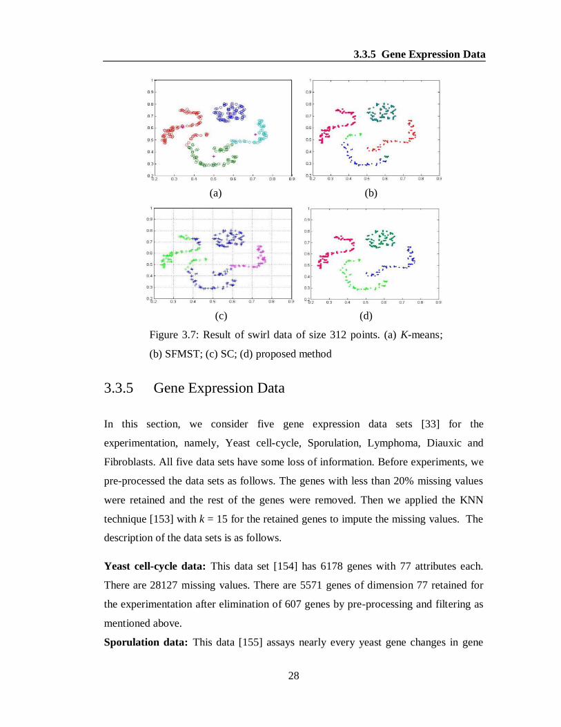
Swirl data: This data set is formed by 312 points and represents 4 clusters, where
each cluster is of different shape. Here, three clusters represent different curves and
one cluster is in spherical shape.
3.3.4 Experimental Results of Synthetic Data
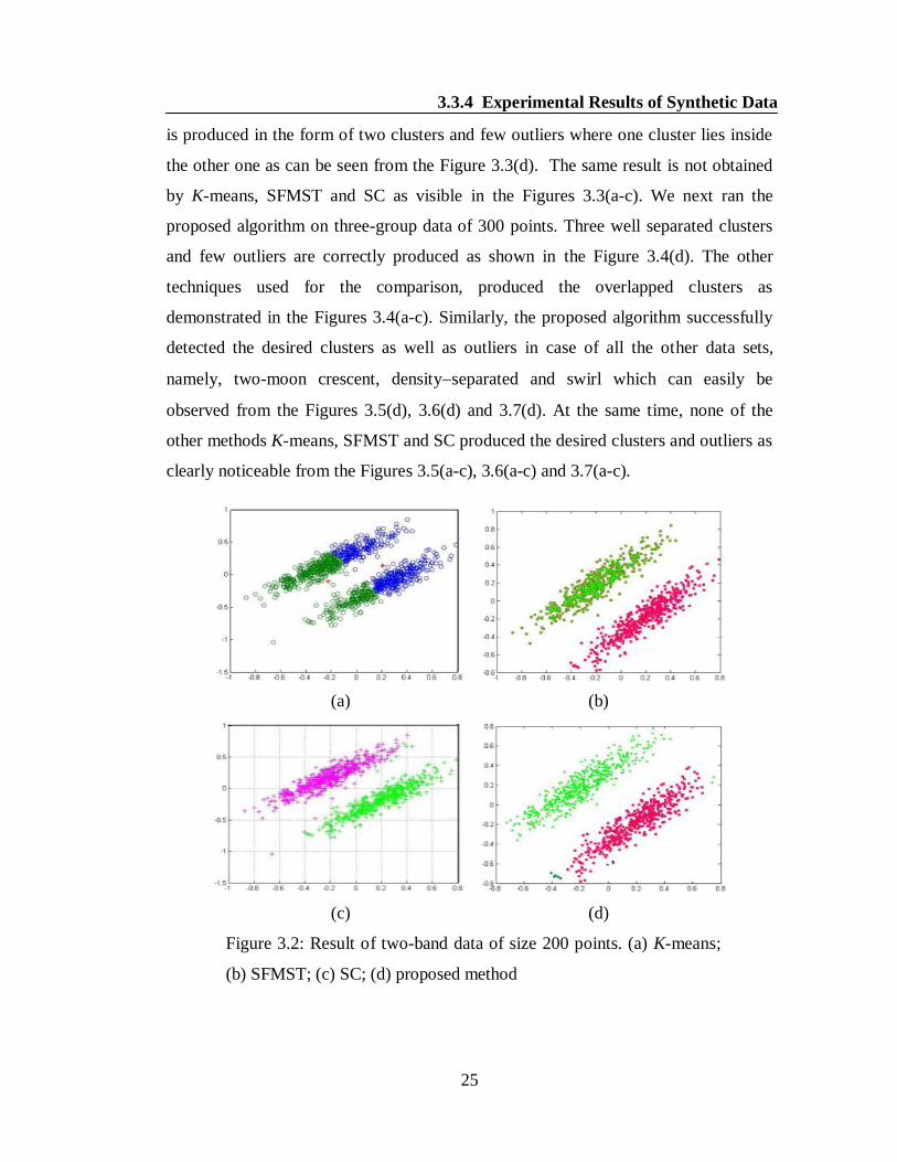
At first we applied the proposed method on the two-band data of size 200 points. The
points of each band are grouped into a separate cluster which is clearly visible from
the Figure 3.2(d). All the points of different clusters are shown by different colors.
The proposed method also located the outliers (small number of points with different
colors) as shown by the same figure. However, the clusters produced by K-means,
SFMST and SC are overlapped as depicted in the Figures 3.2(a-c). The proposed
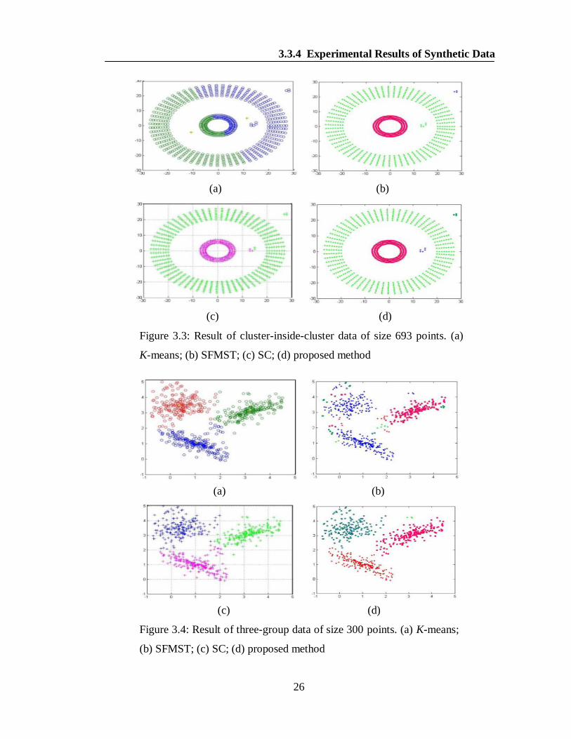
algorithm was next applied on the cluster-inside-cluster data of 693 points. The result
3.3.4 Experimental Results of Synthetic Data
25
is produced in the form of two clusters and few outliers where one cluster lies inside
the other one as can be seen from the Figure 3.3(d). The same result is not obtained
by K-means, SFMST and SC as visible in the Figures 3.3(a-c). We next ran the
proposed algorithm on three-group data of 300 points. Three well separated clusters
and few outliers are correctly produced as shown in the Figure 3.4(d). The other
techniques used for the comparison, produced the overlapped clusters as
demonstrated in the Figures 3.4(a-c). Similarly, the proposed algorithm successfully
detected the desired clusters as well as outliers in case of all the other data sets,
namely, two-moon crescent, densityseparated and swirl which can easily be
observed from the Figures 3.5(d), 3.6(d) and 3.7(d). At the same time, none of the
other methods K-means, SFMST and SC produced the desired clusters and outliers as
clearly noticeable from the Figures 3.5(a-c), 3.6(a-c) and 3.7(a-c).
(a) (b)
(c) (d)
Figure 3.2: Result of two-band data of size 200 points. (a) K-means;
(b) SFMST; (c) SC; (d) proposed method
3.3.4 Experimental Results of Synthetic Data
26
(a) (b)
(c) (d)
Figure 3.3: Result of cluster-inside-cluster data of size 693 points. (a)
K-means; (b) SFMST; (c) SC; (d) proposed method
(a) (b)
(c) (d)
Figure 3.4: Result of three-group data of size 300 points. (a) K-means;
(b) SFMST; (c) SC; (d) proposed method
3.3.4 Experimental Results of Synthetic Data
27
(a) (b)
(c) (d)
Figure 3.5: Result of two-moon crescent data of size 556 points.
(a) K-means; (b) SFMST; (c) SC; (d) proposed method
(a) (b)
(c) (d)
Figure 3.6: Result of density-separated data of size 1009 points.
(a) K-means; (b) SFMST; (c) SC; (d) proposed method
3.3.4 Experimental Results of Synthetic Data
28
(a) (b)
(c) (d)
Figure 3.7: Result of swirl data of size 312 points. (a) K-means;
(b) SFMST; (c) SC; (d) proposed method
3.3.5 Gene Expression Data
In this section, we consider five gene expression data sets [33] for the
experimentation, namely, Yeast cell-cycle, Sporulation, Lymphoma, Diauxic and
Fibroblasts. All five data sets have some loss of information. Before experiments, we
pre-processed the data sets as follows. The genes with less than 20% missing values
were retained and the rest of the genes were removed. Then we applied the KNN
technique [153] with k = 15 for the retained genes to impute the missing values. The
description of the data sets is as follows.
Yeast cell-cycle data: This data set [154] has 6178 genes with 77 attributes each.
There are 28127 missing values. There are 5571 genes of dimension 77 retained for
the experimentation after elimination of 607 genes by pre-processing and filtering as
mentioned above.
Sporulation data: This data [155] assays nearly every yeast gene changes in gene
3.3.5 Gene Expression Data
29
expression during sporulation. It holds a total of 6118 genes of dimension 7 with 612
missing values. After pre-processing 79 genes are removed, and 6039 genes are
retained for the analysis.
Lymphoma data: This data set is used to record the distinct types of diffuse large B-
cell lymphoma identified by gene expression profiling [156]. It has 4026 genes with
96 attributes each. There are 19667 missing values. No genes are removed after pre-
processing and filtering of this data set.
Diauxic data: There are 6153 genes with dimension 7 in Diauxic data [33]. There are
199 missing values and 51 replicates of this data set. After pre-processing the data set
is left with 6100 genes with 7 attributes for each as two genes are removed.
Fibroblasts data: The number of genes of Fibroblasts data [33] is 517 with 18
attributes. There are no missing values of this data set. But 12 replicates have been
located. After pre-processing we finally remain with 501 genes of 18 attributes each.
3.3.6 Experimental Results of Gene Expression Data
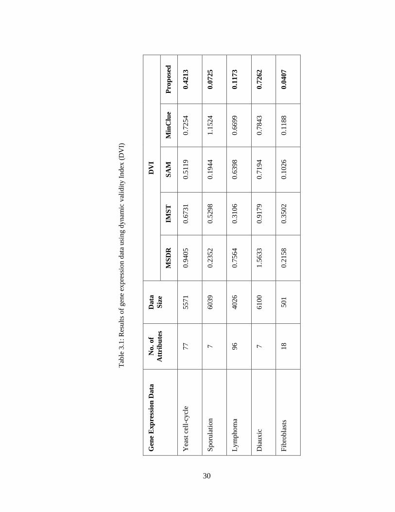
The proposed algorithm was applied on all the above described multi-dimensional
gene expression data sets. For the fair evaluation and without any loss of generality,
the number of clusters was fixed at 256 similar to that of Du et al., [87]. The
performance results of the proposed method and the existing methods MSDR [58],
IMST [49], SAM [64] and MinClue [60] are shown by means of dynamic validity
index (DVI) in Table 3.1. The lower values of DVI indicate more quality of the
clusters. We can easily observe from the Table 3.1 that the proposed MST-based
technique outperforms the algorithms MSDR, IMST, SAM and MinClue.
3.3.6 Experimental Results of Gene Expression Data
30
Tab
le 3
.1:
Res
ult
s of
gen
e ex
pre
ssio
n d
ata
usi
ng d
ynam
ic v
alid
ity I
nd
ex (
DV
I)
DV
I
Pro
po
sed
0.4
21
3
0.0
72
5
0.1
17
3
0.7
26
2
0.0
40
7
Min
Clu
e
0.7
25
4
1.1
52
4
0.6
69
9
0.7
84
3
0.1
18
8
SA
M
0.5
11
9
0.1
94
4
0.6
39
8
0.7
19
4
0.1
02
6
IMS
T
0.6
731
0.5
298
0.3
106
0.9
179
0.3
502
MS
DR
0.9
405
0.2
352
0.7
564
1.5
633
0.2
158
Data
Siz
e
5571
6039
4026
6100
501
No
. of
Att
rib
ute
s
77
7
96
7
18
Gen
e E
xp
ress
ion
Da
ta
Yea
st c
ell-
cycl
e
Sporu
lati
on
Lym
pho
ma
Dia
uxic
Fib
robla
sts
31
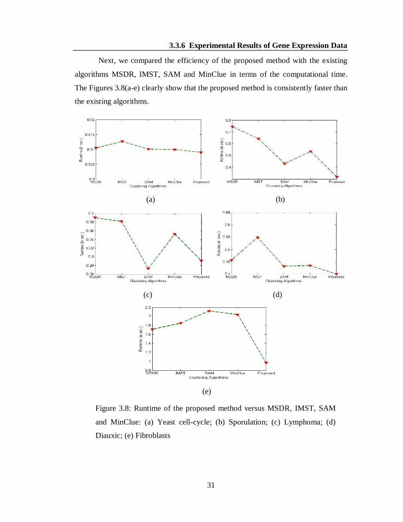
Next, we compared the efficiency of the proposed method with the existing
algorithms MSDR, IMST, SAM and MinClue in terms of the computational time.
The Figures 3.8(a-e) clearly show that the proposed method is consistently faster than
the existing algorithms.
(a) (b)
(c) (d)
(e)
Figure 3.8: Runtime of the proposed method versus MSDR, IMST, SAM
and MinClue: (a) Yeast cell-cycle; (b) Sporulation; (c) Lymphoma; (d)
Diauxic; (e) Fibroblasts
3.3.6 Experimental Results of Gene Expression Data
32
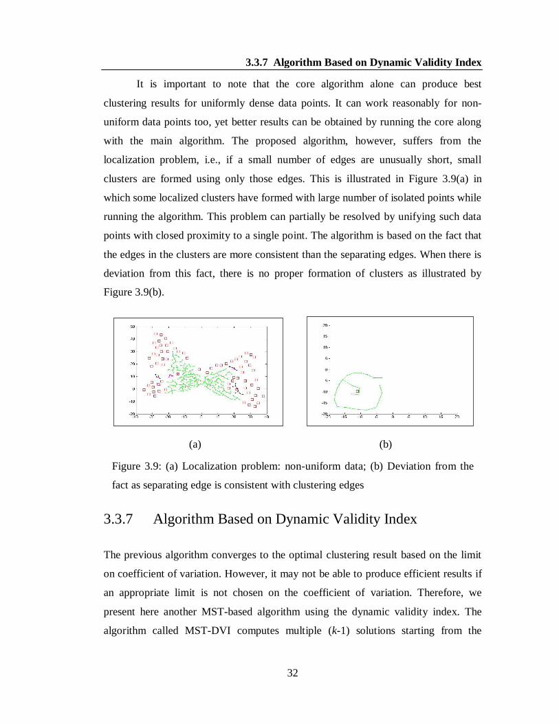
It is important to note that the core algorithm alone can produce best
clustering results for uniformly dense data points. It can work reasonably for non-
uniform data points too, yet better results can be obtained by running the core along
with the main algorithm. The proposed algorithm, however, suffers from the
localization problem, i.e., if a small number of edges are unusually short, small
clusters are formed using only those edges. This is illustrated in Figure 3.9(a) in
which some localized clusters have formed with large number of isolated points while
running the algorithm. This problem can partially be resolved by unifying such data
points with closed proximity to a single point. The algorithm is based on the fact that
the edges in the clusters are more consistent than the separating edges. When there is
deviation from this fact, there is no proper formation of clusters as illustrated by
Figure 3.9(b).
(a) (b)
Figure 3.9: (a) Localization problem: non-uniform data; (b) Deviation from the
fact as separating edge is consistent with clustering edges
3.3.7 Algorithm Based on Dynamic Validity Index
The previous algorithm converges to the optimal clustering result based on the limit
on coefficient of variation. However, it may not be able to produce efficient results if
an appropriate limit is not chosen on the coefficient of variation. Therefore, we
present here another MST-based algorithm using the dynamic validity index. The
algorithm called MST-DVI computes multiple (k-1) solutions starting from the
3.3.7 Algorithm Based on Dynamic Validity Index
33
highest weight of the MST. Finally, the optimal solution is picked up from the k-1
solutions. The main idea of this method is as follows. We first construct the MST
from the given data set using Prim’s algorithm. Then we go on removing the edges in
the decreasing order of their weights. At each removal of the next highest edge, it
results into certain number of clusters. If any cluster has data points beyond some
minimum number, we treat it as an outlier and we do not consider it as a valid cluster.
Then we calculate the DVI with the valid clusters only and record both the value of
the DVI and the number of clusters. The same process is repeated until some criterion
is satisfied. We obtain the final clusters corresponding to the minimum value of the
DVI recorded. The algorithm is formally presented stepwise as follows.
Algorithm MST-DVI (S, C)
Input: A set S of the given data points and a parameter C lies between 0 and 1.
Output: Clusters C1, C2,…, Ck.
Functions and variables used:
k: A variable to represent the number of clusters
C: A parameter lies between 0 and 1
DVI (C1, C2,…, Ck): A function to find the dynamic validity index of the clusters C1,
C2,…, Ck
Step 1: Construct the minimum spanning tree for the given data points using Prim’s
algorithm.
Step 2: Set initial value of number of clusters, i.e., k 1.
/* Assume that initially whole MST is a cluster */
Step 3: Remove the edge with greatest weight in the MST to produce the clusters.
Step 4: Increase the value of k by 1, i.e., k k + 1.
Step 5: Check for each cluster (formed in step 3) whether it contains minimum data
points for it to be a valid cluster.
/* This step is basically for the outlier detection */
34
Step 6: For each invalid cluster (outlier) if any, decrease value of k by 1.
i.e., set k k 1.
Step 7: Call DVI (C1, C2,…, Ck) to calculate dynamic validity index by considering k
valid clusters using the below formula:
)}(*)({,,2,1
min),,2
,1
( jInterRatiojIntraRatiokjk
CCCDVI
Step 8: Record the value of DVI calculated in step 7 and the corresponding k value.
Step 9: Repeat from step 3 until the termination criterion D(n) > C * D(p) is met,
where C is the parameter that lies between 0 to1, D(n) is the length of the
current edge to be removed for cluster formation and D(p) is the length of the
edge previously removed.
Step 10: Obtain the k clusters with respect to the minimum value of the DVI from
step 8.
Step 11: Stop.
Time Complexity: The minimum spanning tree is constructed in O (n2) time using
Prim’s algorithm. The value of the dynamic validity index (DVI) is computed for k +
1 times in O ((k + 1)n) time. Therefore, the total computational cost of the proposed
algorithm is quadratic.
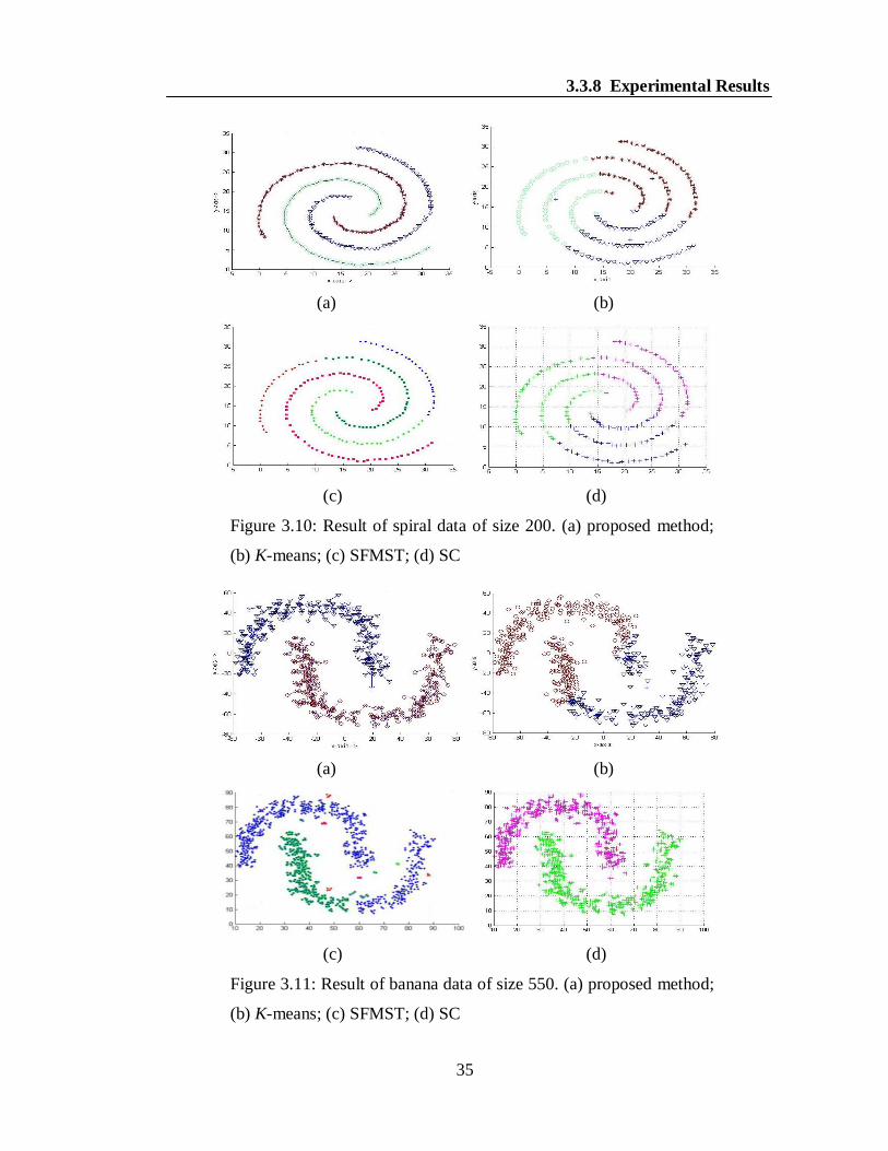
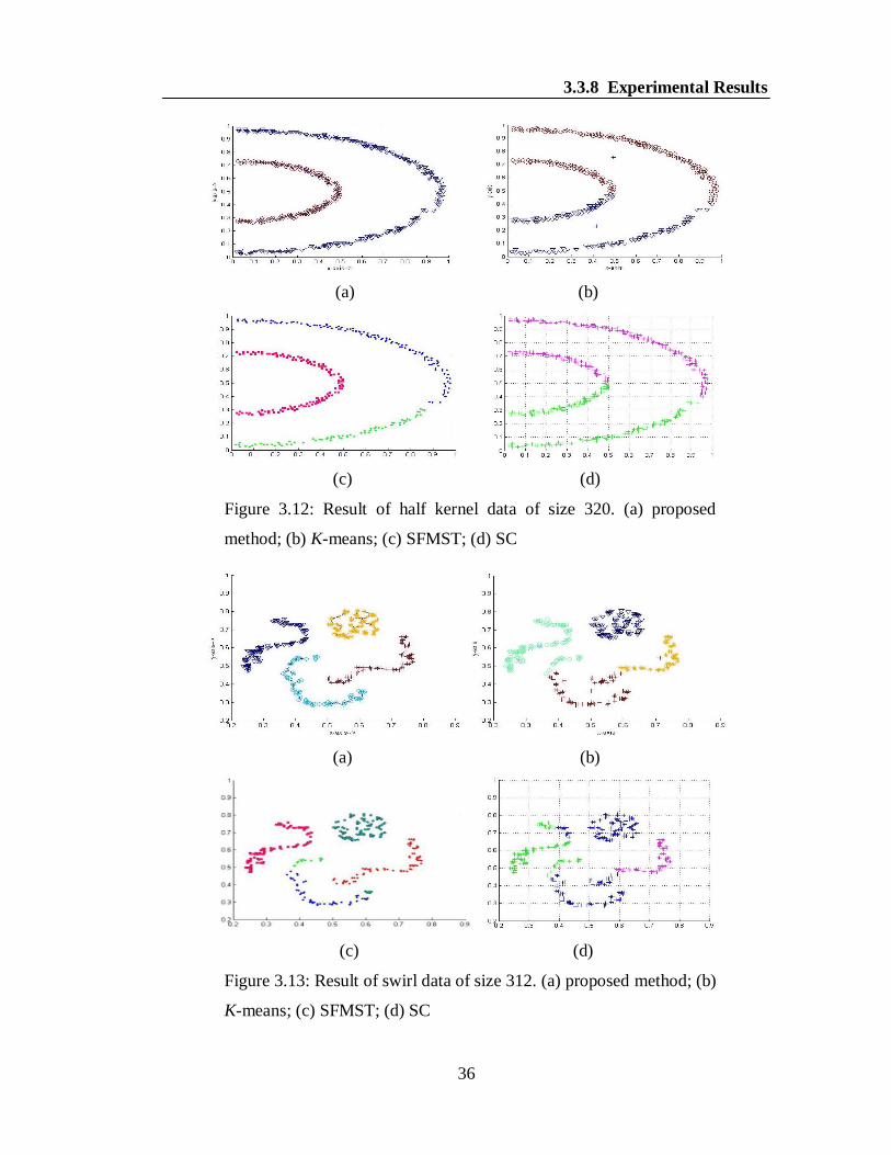
3.3.8 Experimental Results
For experiments, we considered four synthetic data sets, namely spiral, banana, half
kernel and swirl data. The results are shown in Figures 3.10(a-d)-3.13(a-d). In a
specific figure, different clusters are shown by different colors for the better
visualization. It is obvious to note from the Figures 3.10(a), 3.11(a), 3.12(a) and
3.13(a) that our algorithm is able to produce the desired clusters for all the synthetic
data where as the K-means, SFMST and SC produces the clusters in overlapped
fashion as shown in the Figures 3.10(b-d), 3.11(b-d), 3.12(b-d) and 3.13(b-d). It can
be noted that the algorithm SC also produced similar result in case of banana data.
35
(a) (b)
(c) (d)
Figure 3.10: Result of spiral data of size 200. (a) proposed method;
(b) K-means; (c) SFMST; (d) SC
(a) (b)
(c) (d)
Figure 3.11: Result of banana data of size 550. (a) proposed method;
(b) K-means; (c) SFMST; (d) SC
3.3.8 Experimental Results
36
(a) (b)
(c) (d)
Figure 3.12: Result of half kernel data of size 320. (a) proposed
method; (b) K-means; (c) SFMST; (d) SC
(a) (b)
(c) (d)
Figure 3.13: Result of swirl data of size 312. (a) proposed method; (b)
K-means; (c) SFMST; (d) SC
3.3.8 Experimental Results

37
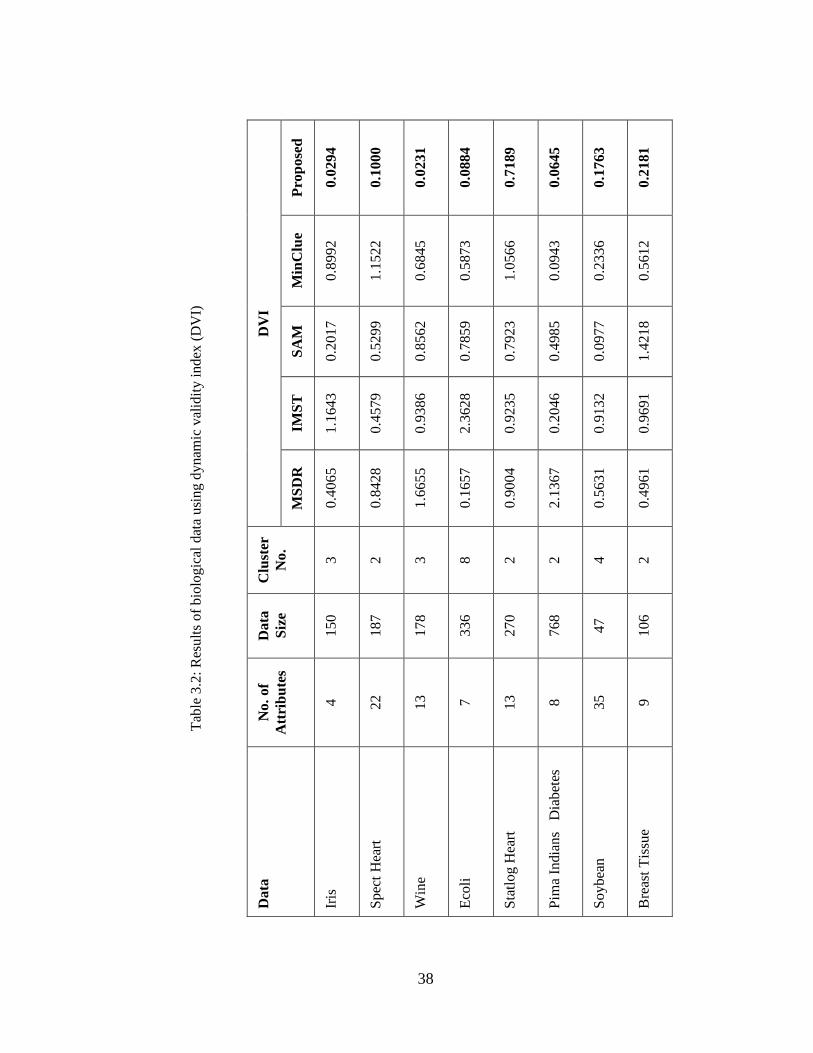
Next, we tested the algorithm on eight biological data sets [32], namely iris,
spect heart, wine, ecoli, statlog heart, Pima Indians diabetes, soybean and breast
tissue with dimensions 4, 22, 13, 7, 13, 8, 35 and 9 respectively. The experimental
results and their comparisons with respect to the DVI [151] values are shown in Table
3.2. It can be noted that our algorithm has better (lower) DVI values than that of
MSDR [58], IMST [49], SAM [64] and MinClue [60] algorithms in case of most of
the biological data.
3.3.8 Experimental Results
38
Tab
le 3
.2:
Res
ult
s of
bio
logic
al d
ata
usi
ng d
ynam
ic v
alid
ity i
nd
ex (
DV
I)
DV
I
Pro
po
sed
0
.02
94
0.1
00
0
0.0
23
1
0.0
88
4
0.7
18
9
0.0
64
5
0.1
76
3
0.2
18
1
Min
Clu
e
0
.89
92
1.1
52
2
0.6
84
5
0.5
87
3
1.0
56
6
0.0
94
3
0.2
33
6
0.5
61
2
SA
M
0
.20
17
0.5
29
9
0.8
56
2
0.7
85
9
0.7
92
3
0.4
98
5
0.0
97
7
1.4
21
8
IMS
T
1.1
643
0.4
579
0.9
386
2.3
628
0.9
235
0.2
046
0.9
132
0.9
691
MS
DR
0.4
065
0.8
428
1.6
655
0.1
657
0.9
004
2.1
367
0.5
631
0.4
961
Clu
ster
No.
3
2
3
8
2
2
4
2
Data
Siz
e
150
187
178
336
270
768
47
106
No.
of
Att
rib
ute
s
4
22
13
7
13
8
35
9
Data
Iris
Spec
t H
eart
Win
e
Eco
li
Sta
tlo
g H
eart
Pim
a In
dia
ns
D
iab
etes
Soybea
n
Bre
ast
Tis
sue
39
3.4 Conclusion
In this chapter, we presented two MST-based algorithms which run with quadratic
computational complexity. Initially, a novel algorithm called MST-CV has been
presented based on the coefficient of variation. It is shown to be effective for various
two dimensional synthetic and multi-dimensional gene expression data such as Yeast
cell-cycle, Sporulation, Lymphoma, Diauxic and Fibroblasts. The results of the
proposed method on the synthetic data are shown to be better than K-means, SFMST
and SC algorithms. Similarly, in case of gene expression data, the algorithm MST-
CV outperforms MSDR, IMST, SAM and MinClue in terms of DVI. It is observed
that our algorithm has low computational cost over the existing. Next, another MST-
based clustering algorithm named MST-DVI has been proposed. This technique
eliminates the inconsistent edges with the help of dynamic validity index. This
method is also able to deal with the outlier points. This algorithm is experimented on
several synthetic and biological data, namely, iris, spect heart, wine, ecoli, statlog
heart, Pima Indians diabetes, soybean and breast tissue. The results of the synthetic
data are compared with the K-means, SFMST and SC methods and the results of the
proposed scheme on biological data are compared with the existing clustering
techniques MSDR, IMST, SAM and MinClue using DVI. The algorithm MST-DVI
produced efficient results than that of the existing methods.
3.4 Conclusion
Top Related