


Languages
Pages
Legal

Chapter 2, Part 1
FIRST ORDER EQUATIONS
F (x, y, y′) = 0
Basic assumption: The equation
can be solved for y′; that is, the
equation can be written in the form
y′ = f(x, y) (1)
1
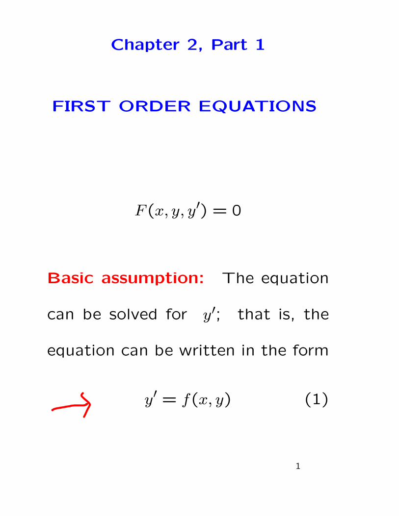
2.1. First Order Linear Equa-
tions
Equation (1) is a linear equation if
f has the form
f(x, y) = P (x)y + q(x)
where P and q are continuous
functions on some interval I. Thus
y′ = P (x)y + q(x)
2
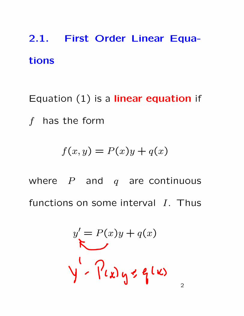
Standard form:
The standard form for a first order
linear equation is:
y′ + p(x)y = q(x)
where p and q are continuous
functions on the interval I
(Note: A differential equation which
is not linear is called nonlinear.)
3
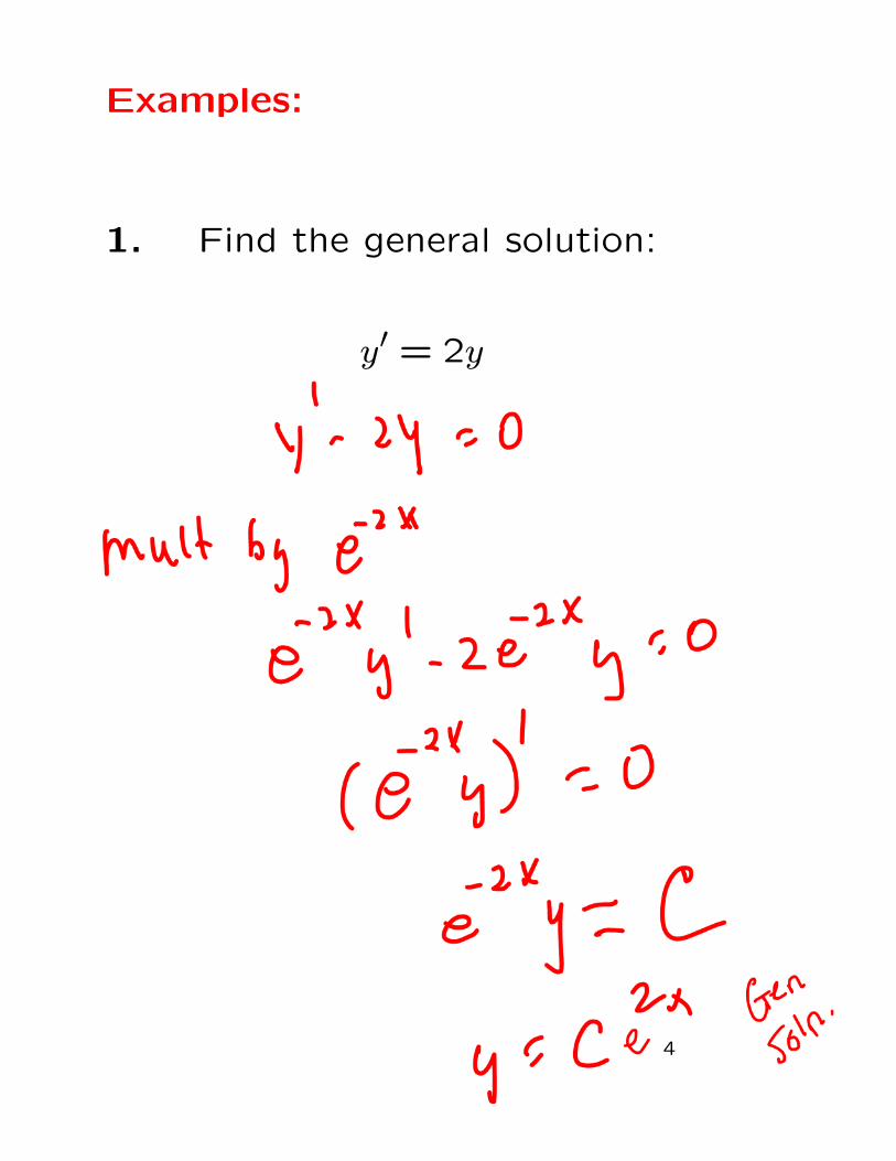
Examples:
1. Find the general solution:
y′ = 2y
4
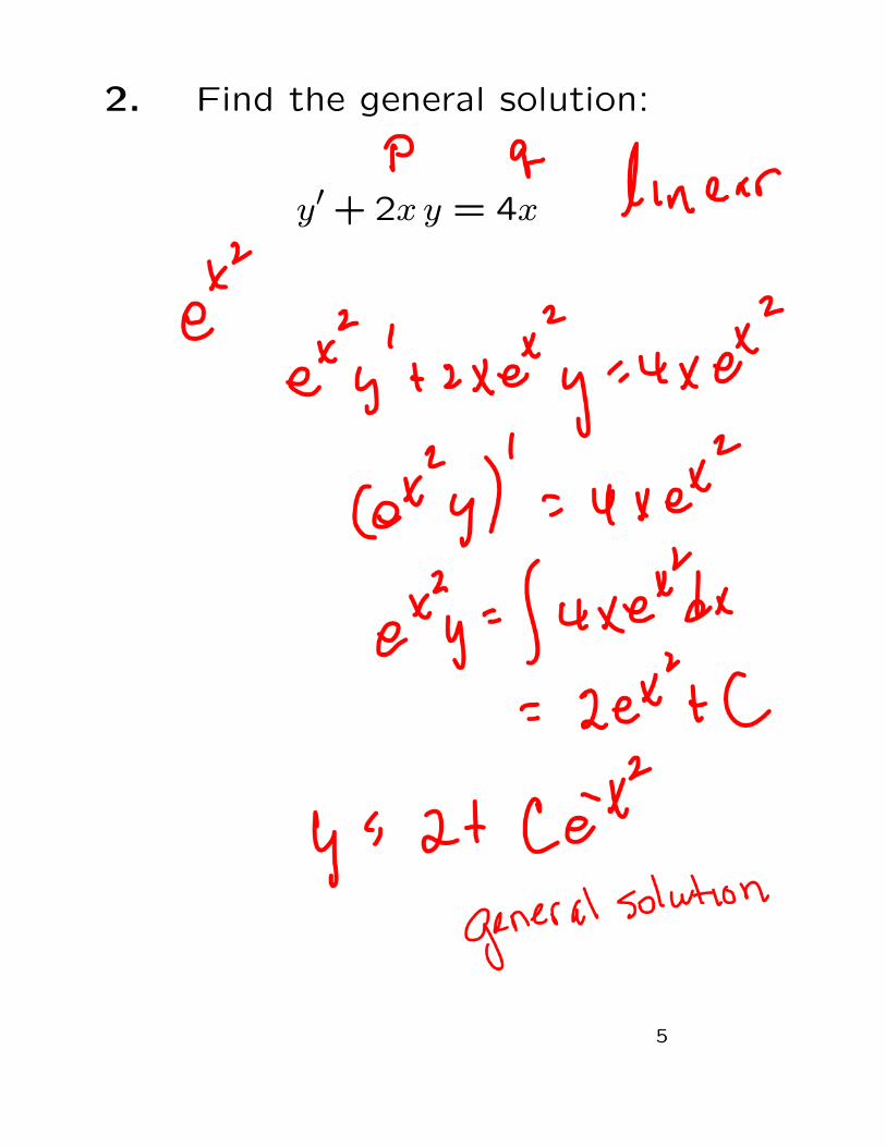
2. Find the general solution:
y′ + 2x y = 4x
5
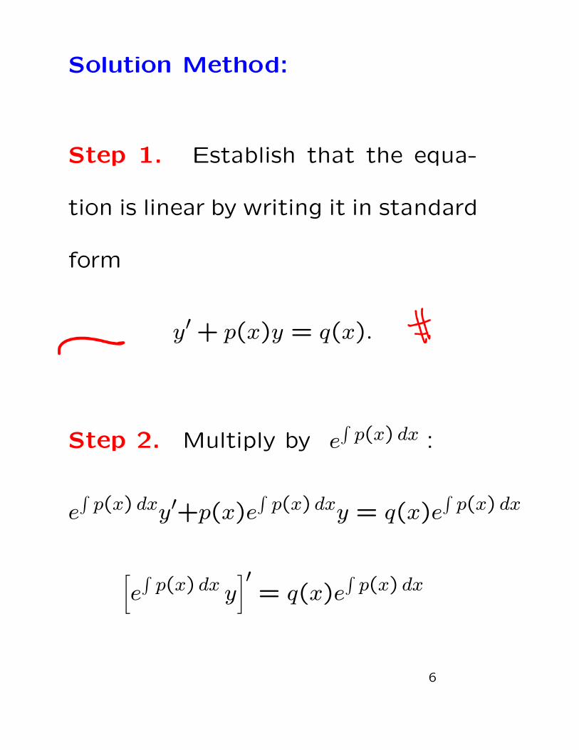
Solution Method:
Step 1. Establish that the equa-
tion is linear by writing it in standard
form
y′ + p(x)y = q(x).
Step 2. Multiply by e∫
p(x) dx :
e∫
p(x) dxy′+p(x)e∫
p(x) dxy = q(x)e∫
p(x) dx
[
e∫
p(x) dx y]′
= q(x)e∫
p(x) dx
6
[
e∫
p(x) dx y]′
= q(x)e∫
p(x) dx
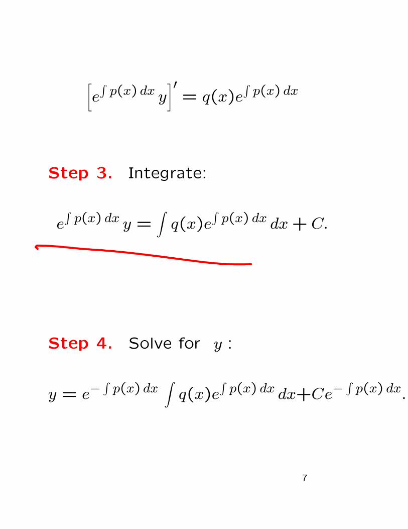
Step 3. Integrate:
e∫
p(x) dx y =∫
q(x)e∫
p(x) dx dx + C.
Step 4. Solve for y :
y = e−∫
p(x) dx∫
q(x)e∫
p(x) dx dx+Ce−∫
p(x) dx.
7

y = e−∫
p(x) dx∫
q(x)e∫
p(x) dx dx+Ce−∫
p(x) dx.
is the general solution of the equa-
tion.
Note: e∫
p(x) dx is called an inte-
grating factor
8
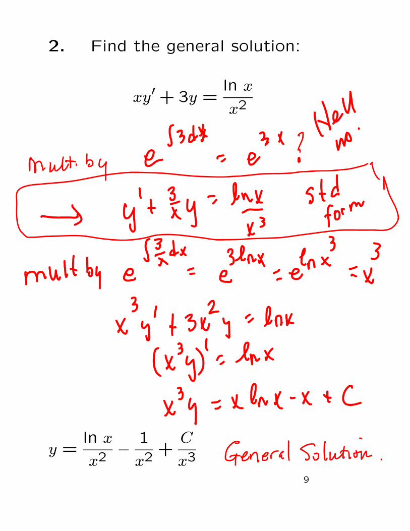
2. Find the general solution:
xy′ + 3y =ln x
x2
y =ln x
x2− 1
x2+
C
x3
9
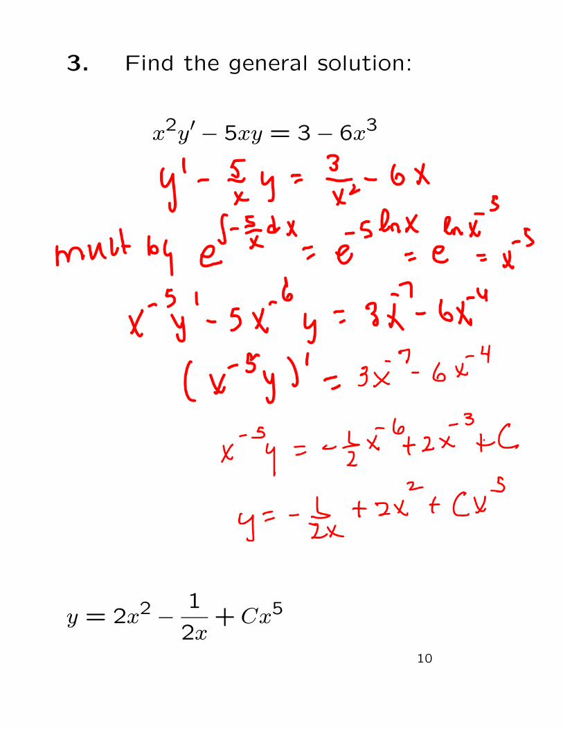
3. Find the general solution:
x2y′ − 5xy = 3 − 6x3
y = 2x2 − 1
2x+ Cx5
10
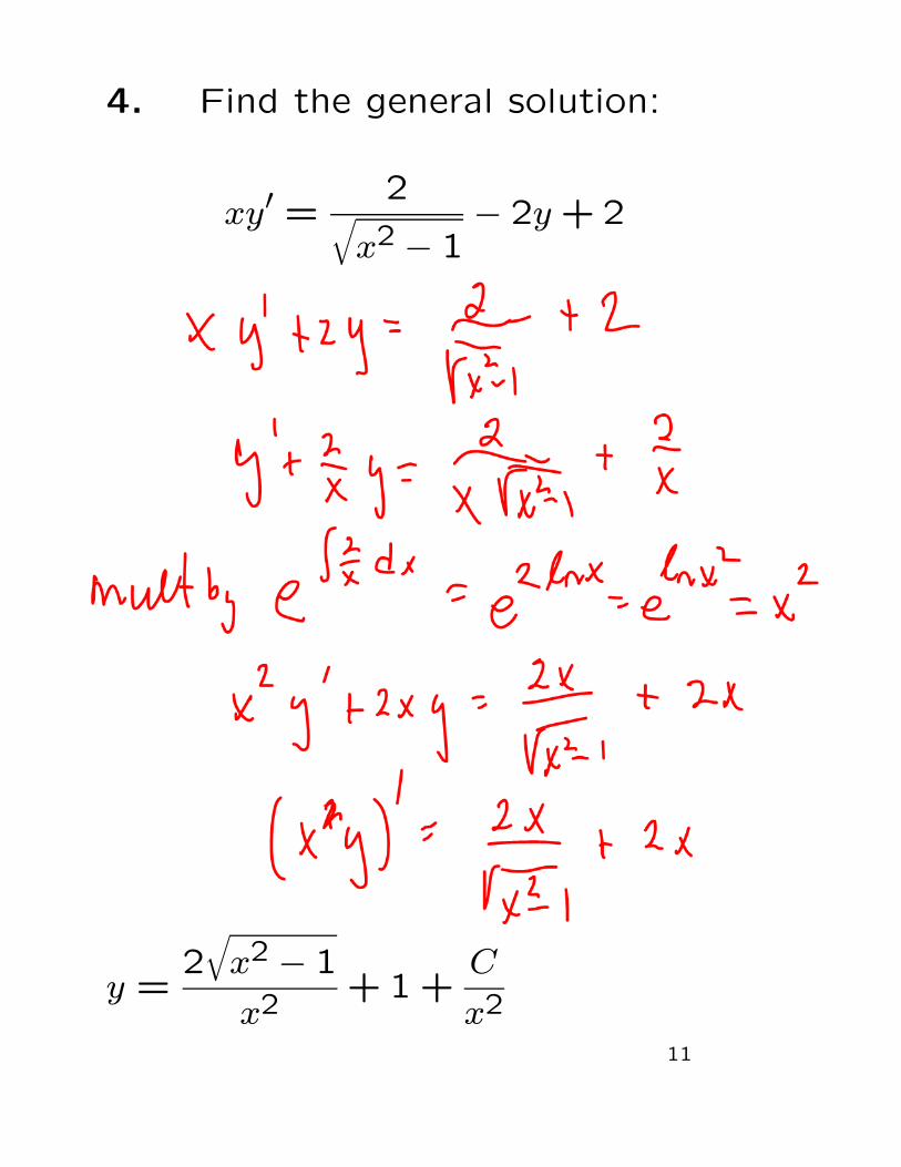
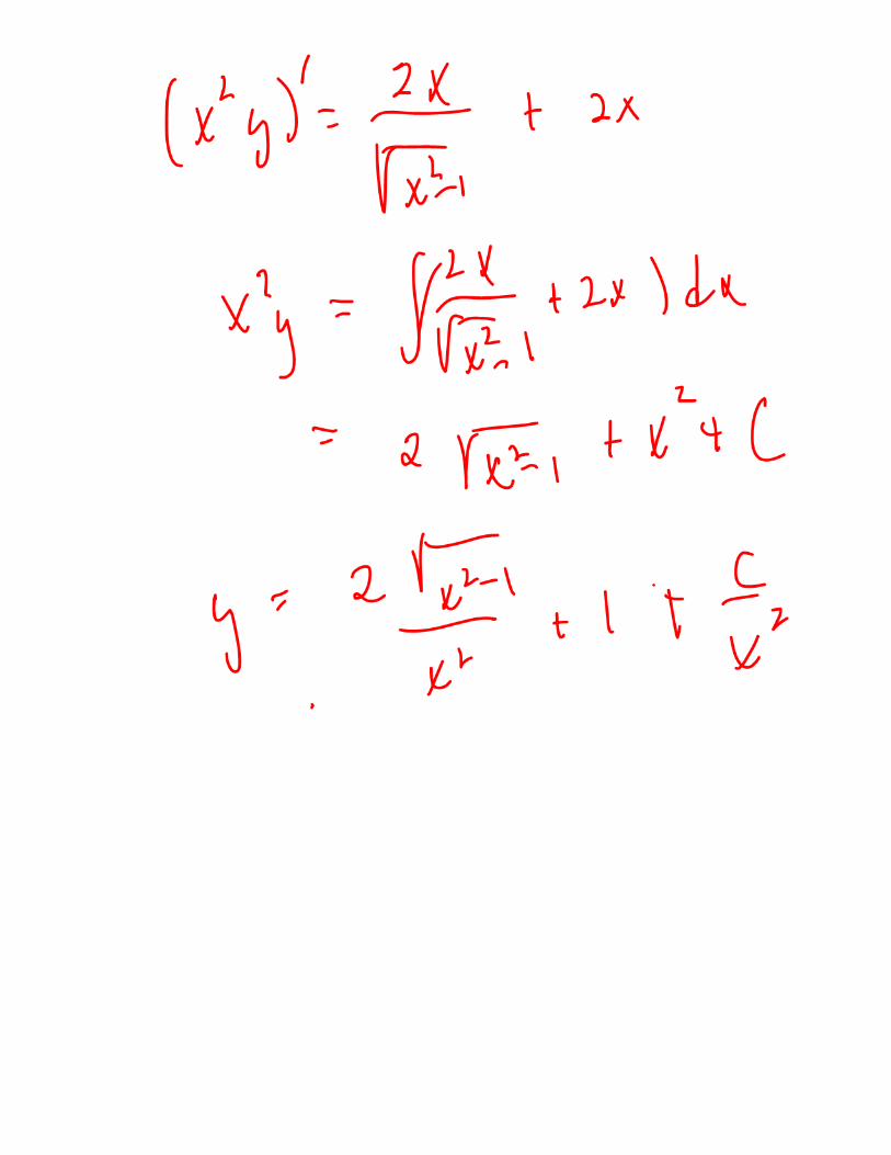
4. Find the general solution:
xy′ =2
√
x2 − 1− 2y + 2
y =2
√
x2 − 1
x2+ 1 +
C
x2
11
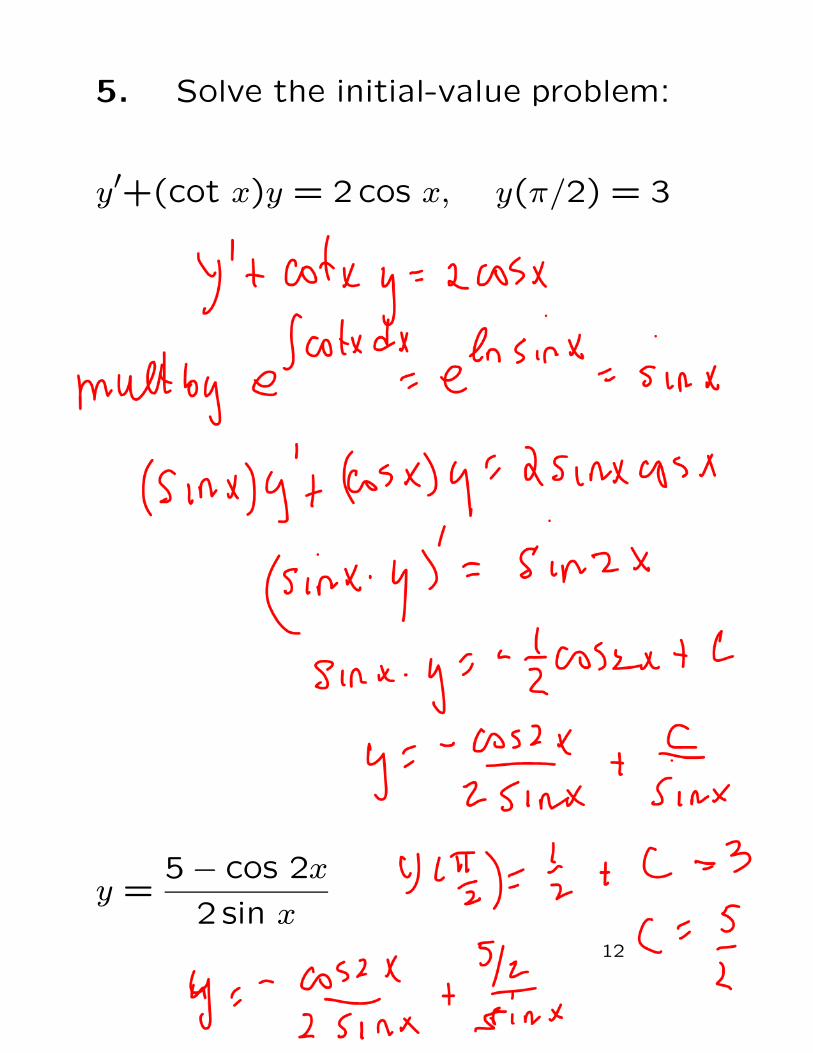
5. Solve the initial-value problem:
y′+(cot x)y = 2cos x, y(π/2) = 3
y =5 − cos 2x
2 sin x12
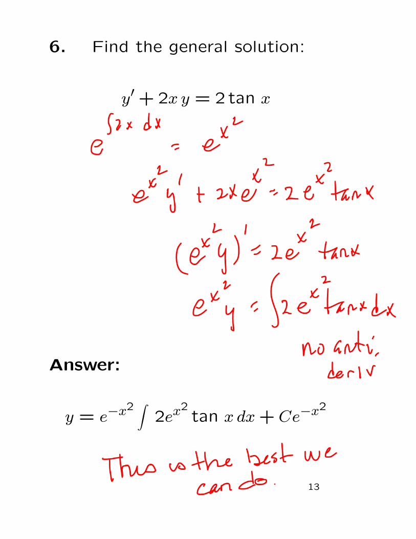
6. Find the general solution:
y′ + 2x y = 2tan x
Answer:
y = e−x2∫
2ex2tan x dx + Ce−x2
13
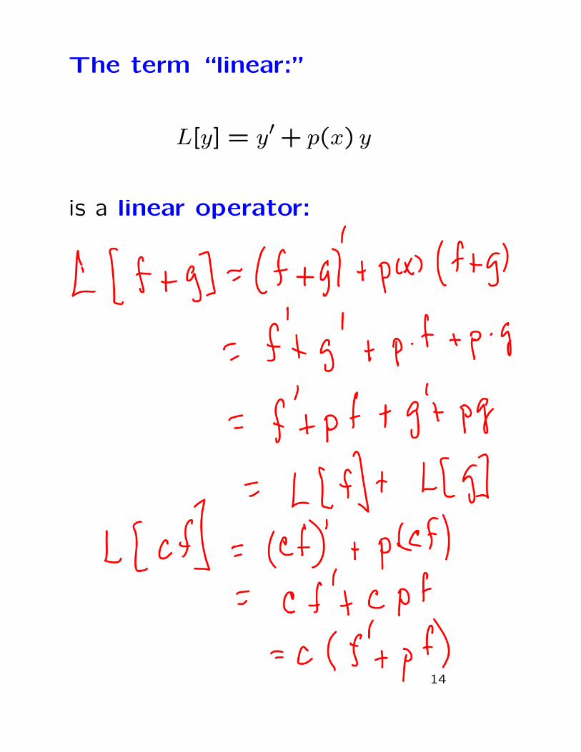
The term “linear:”
L[y] = y′ + p(x) y
is a linear operator:
14
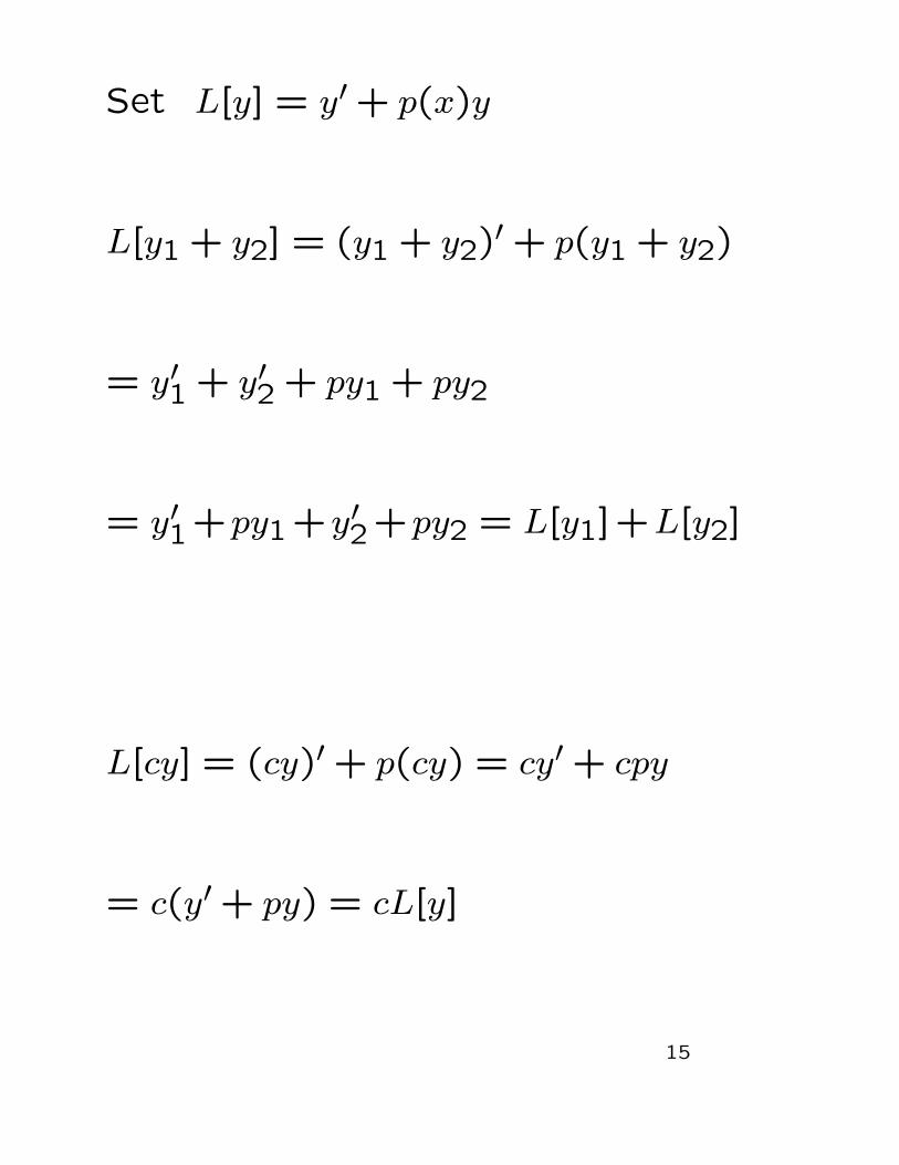
Set L[y] = y′ + p(x)y
L[y1 + y2] = (y1 + y2)′ + p(y1 + y2)
= y′1 + y′2 + py1 + py2
= y′1+py1+y′2+py2 = L[y1]+L[y2]
L[cy] = (cy)′ + p(cy) = cy′ + cpy
= c(y′ + py) = cL[y]
15
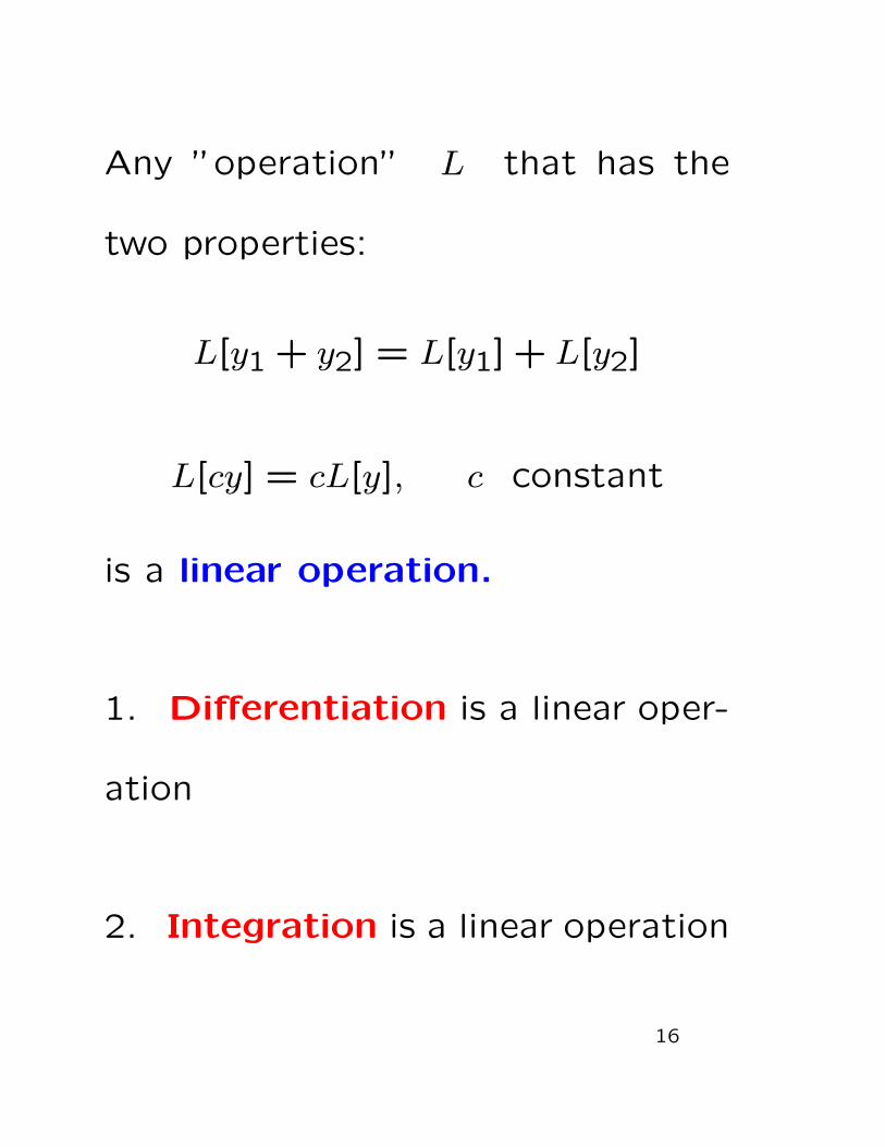
Any ”operation” L that has the
two properties:
L[y1 + y2] = L[y1] + L[y2]
L[cy] = cL[y], c constant
is a linear operation.
1. Differentiation is a linear oper-
ation
2. Integration is a linear operation
16

3. L[y] = y + p(x)y is a linear op-
eration.
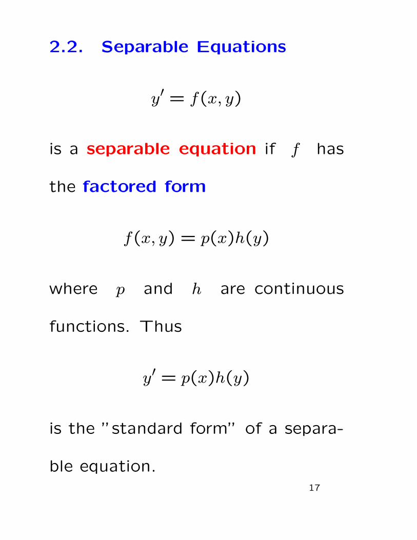
2.2. Separable Equations
y′ = f(x, y)
is a separable equation if f has
the factored form
f(x, y) = p(x)h(y)
where p and h are continuous
functions. Thus
y′ = p(x)h(y)
is the ”standard form” of a separa-
ble equation.17
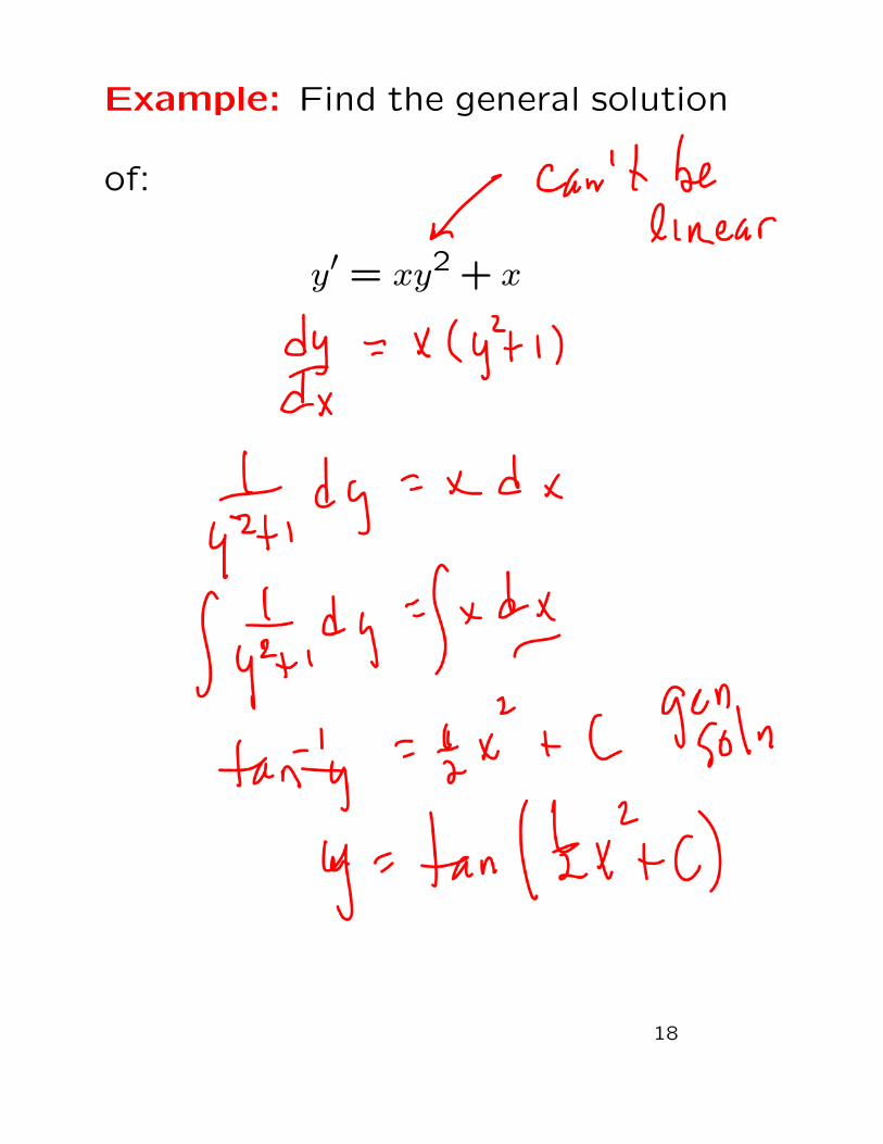
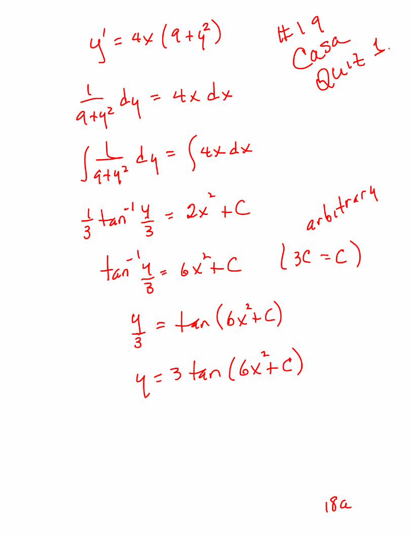
Example: Find the general solution
of:
y′ = xy2 + x
18
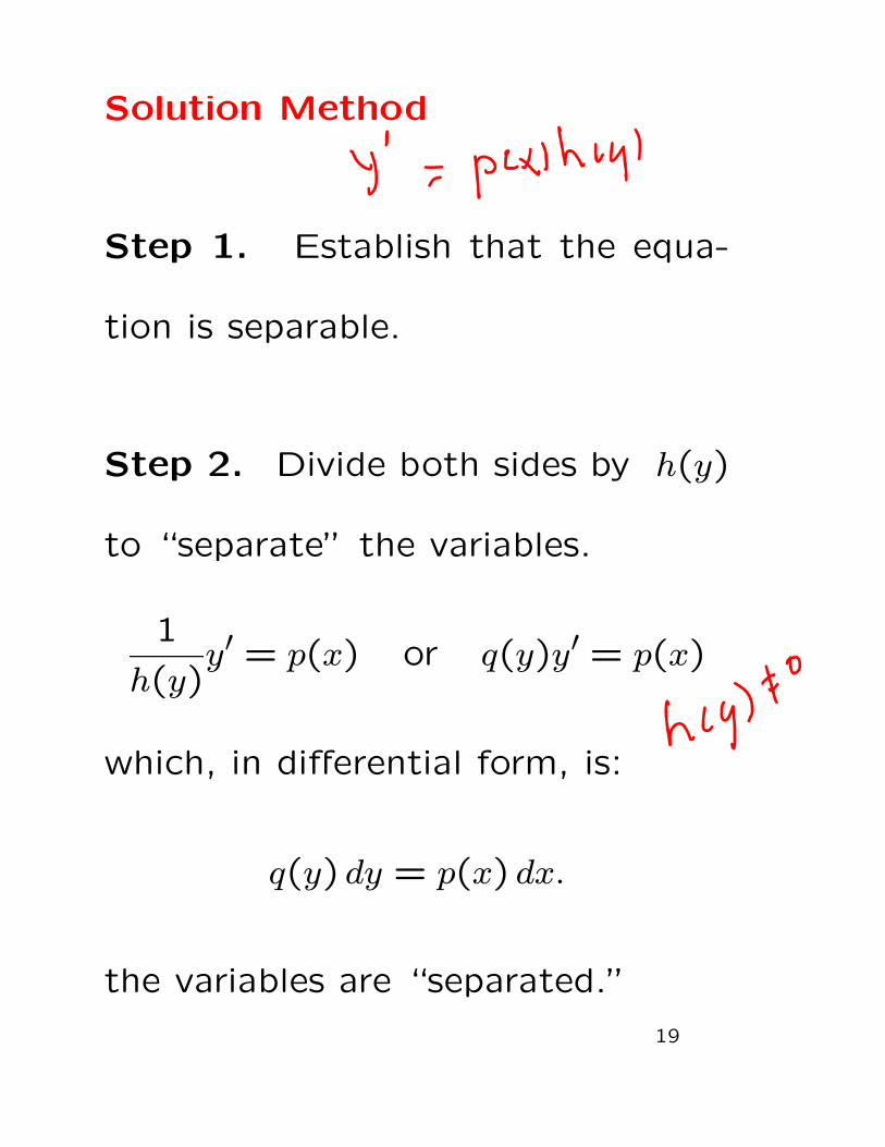
Solution Method
Step 1. Establish that the equa-
tion is separable.
Step 2. Divide both sides by h(y)
to “separate” the variables.
1
h(y)y′ = p(x) or q(y)y′ = p(x)
which, in differential form, is:
q(y) dy = p(x) dx.
the variables are “separated.”
19
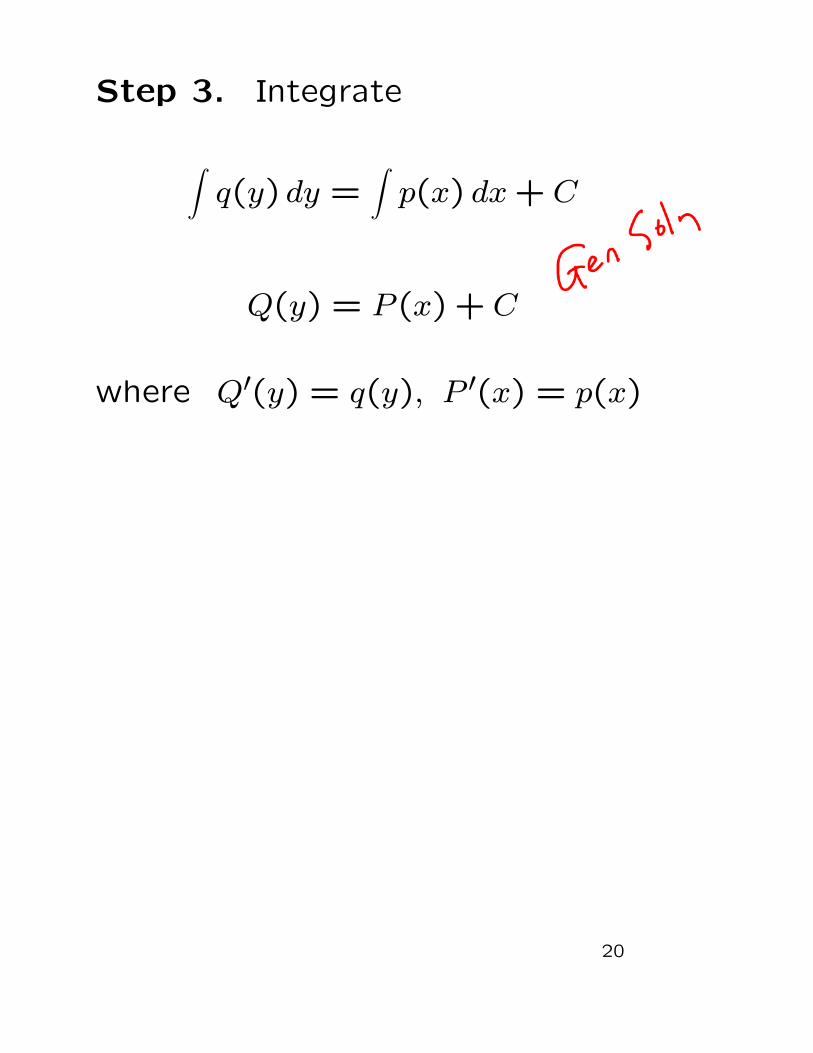
Step 3. Integrate
∫
q(y) dy =∫
p(x) dx + C
Q(y) = P (x) + C
where Q′(y) = q(y), P ′(x) = p(x)
20
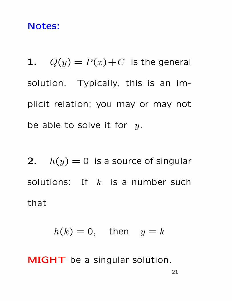
Notes:
1. Q(y) = P (x)+C is the general
solution. Typically, this is an im-
plicit relation; you may or may not
be able to solve it for y.
2. h(y) = 0 is a source of singular
solutions: If k is a number such
that
h(k) = 0, then y = k
MIGHT be a singular solution.21

Examples:
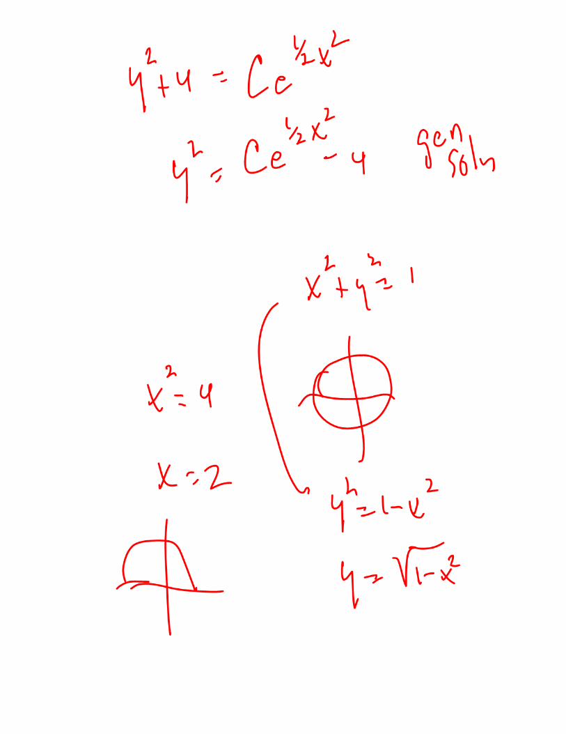
1. Find the general solution:
y′ =2xy2 + 8x
4y
22
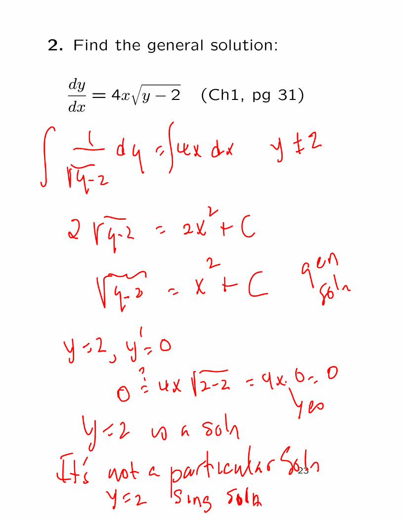
2. Find the general solution:
dy
dx= 4x
√
y − 2 (Ch1, pg 31)
23
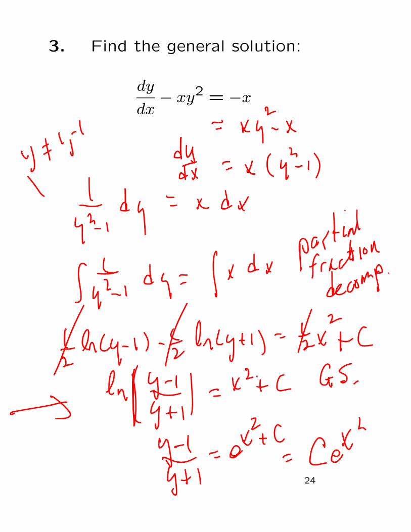
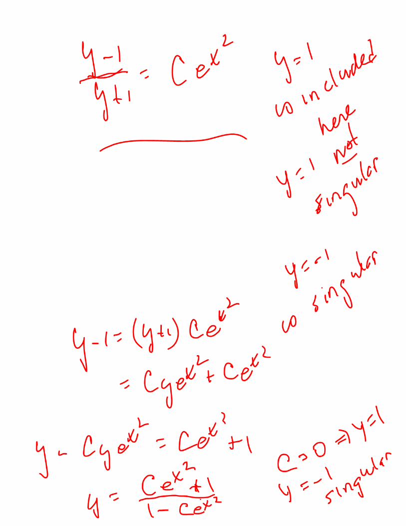
3. Find the general solution:
dy
dx− xy2 = −x
24
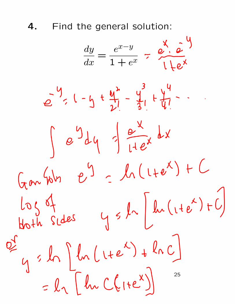
4. Find the general solution:
dy
dx=
ex−y
1 + ex
25
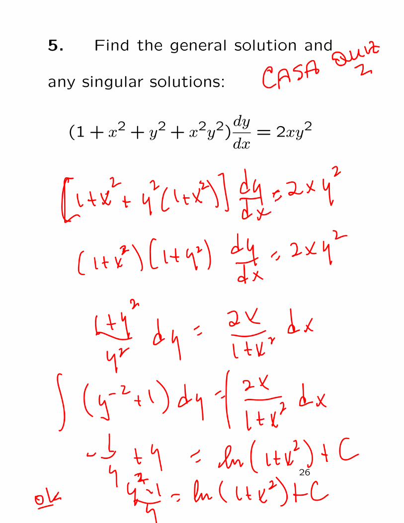
5. Find the general solution and
any singular solutions:
(1 + x2 + y2 + x2y2)dy
dx= 2xy2
26

2.3. Related Equations & Trans-
formations
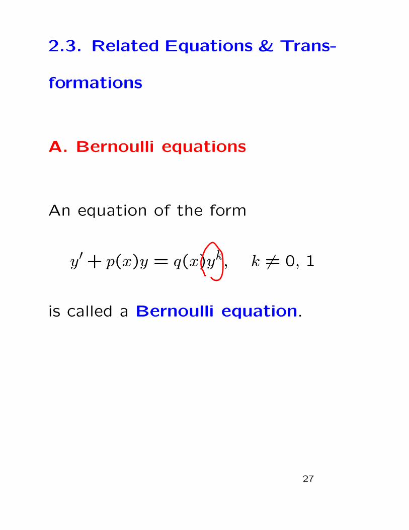
A. Bernoulli equations
An equation of the form
y′ + p(x)y = q(x)yk, k 6= 0, 1
is called a Bernoulli equation.
27
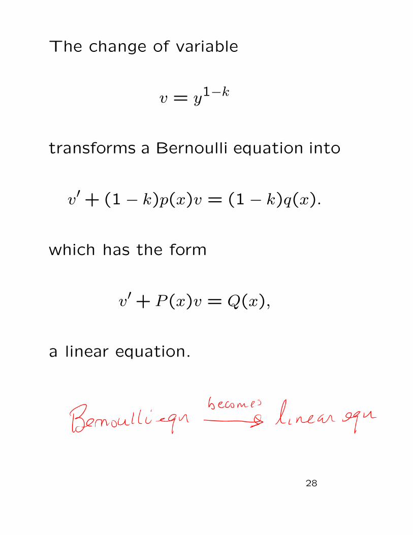
The change of variable
v = y1−k
transforms a Bernoulli equation into
v′ + (1 − k)p(x)v = (1 − k)q(x).
which has the form
v′ + P (x)v = Q(x),
a linear equation.
28
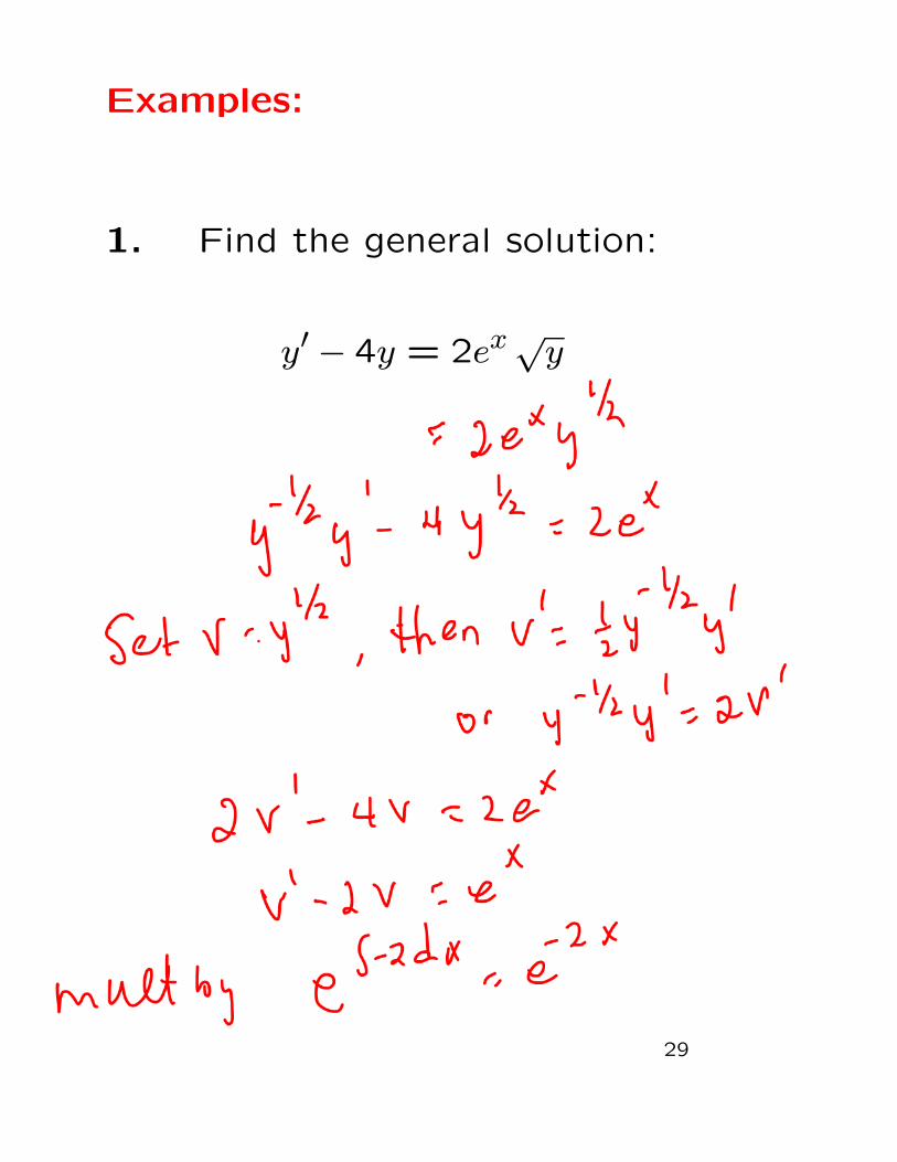
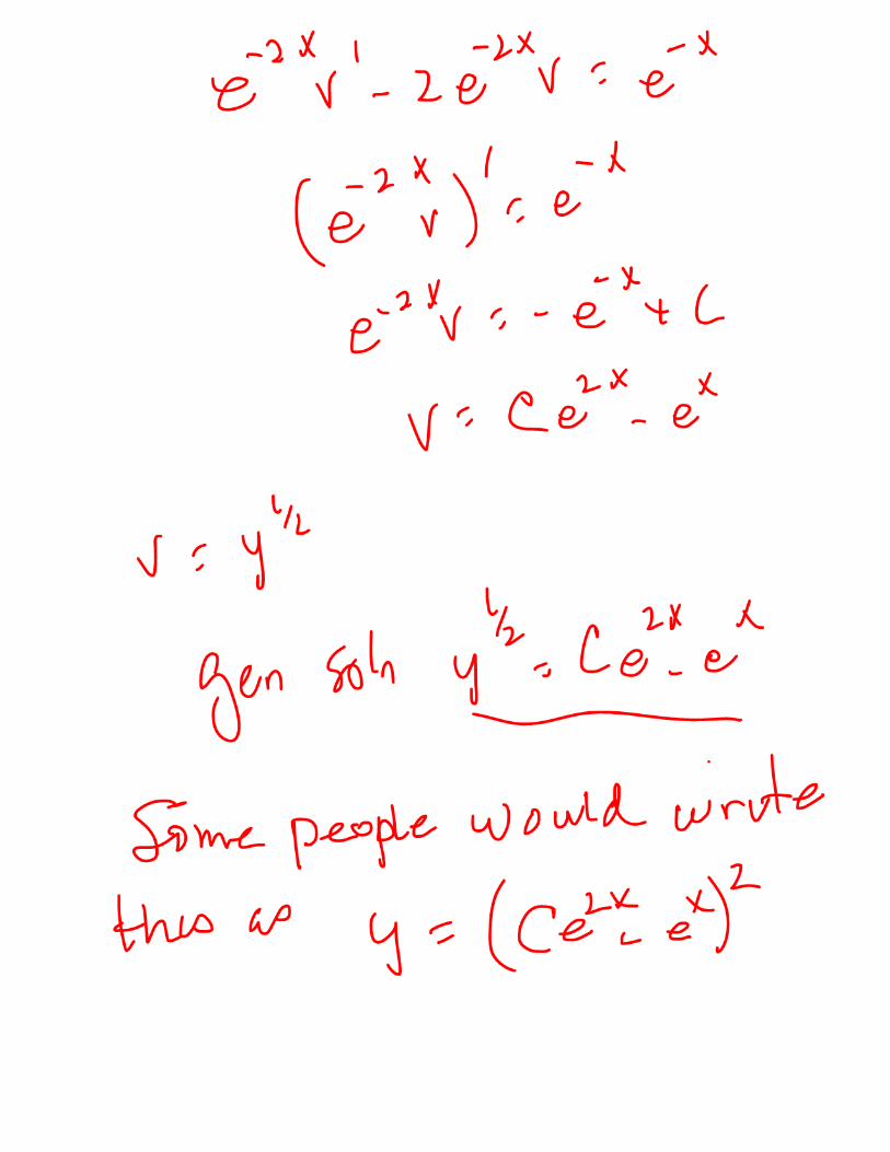
Examples:
1. Find the general solution:
y′ − 4y = 2ex √y
29
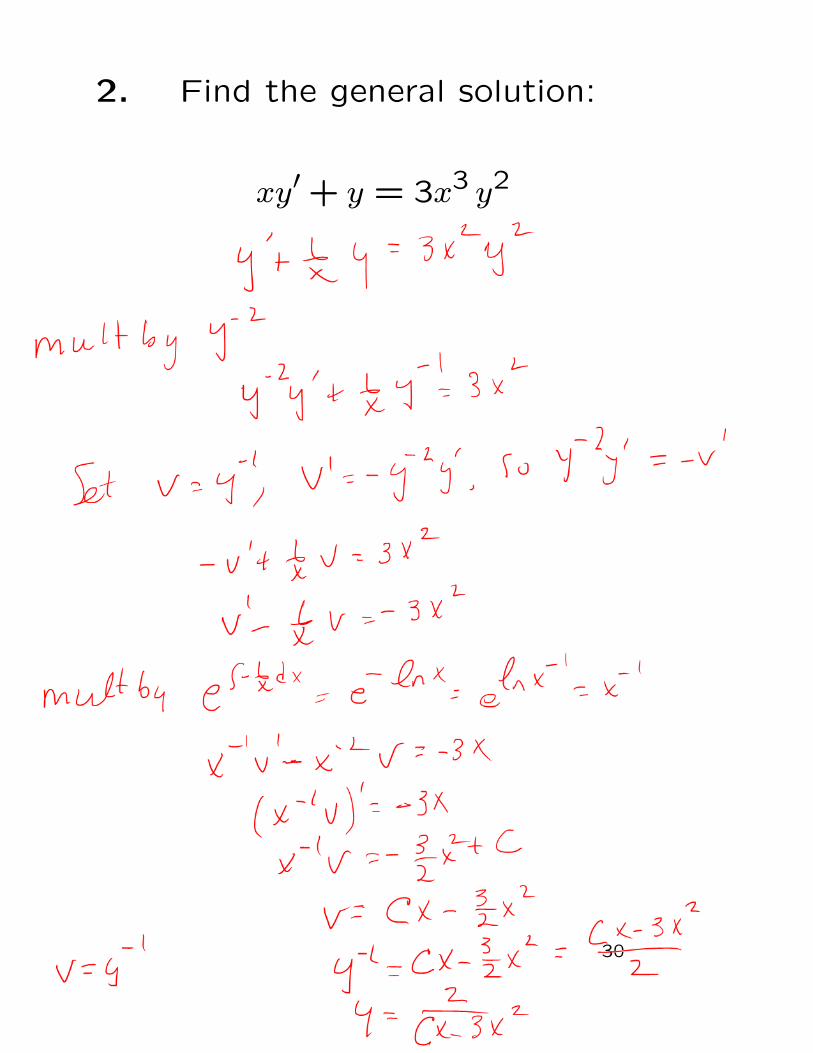
2. Find the general solution:
xy′ + y = 3x3 y2
30
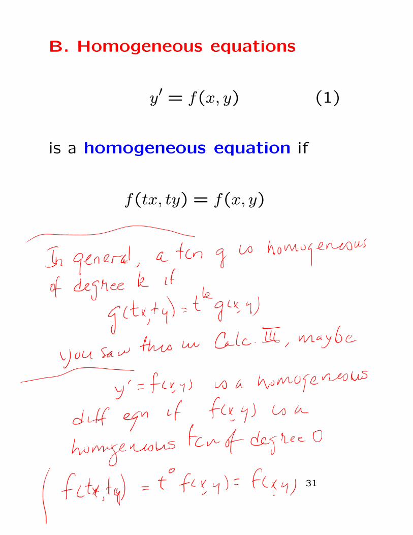
B. Homogeneous equations
y′ = f(x, y) (1)
is a homogeneous equation if
f(tx, ty) = f(x, y)
31
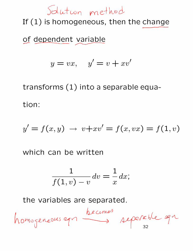
If (1) is homogeneous, then the change
of dependent variable
y = vx, y′ = v + xv′
transforms (1) into a separable equa-
tion:
y′ = f(x, y) → v+xv′ = f(x, vx) = f(1, v)
which can be written
1
f(1, v) − vdv =
1
xdx;
the variables are separated.
32

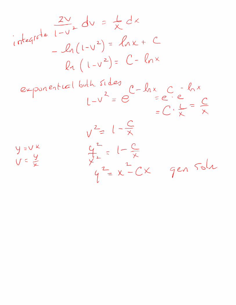
Examples:
1. Find the general solution:
y′ =x2 + y2
2xy
33
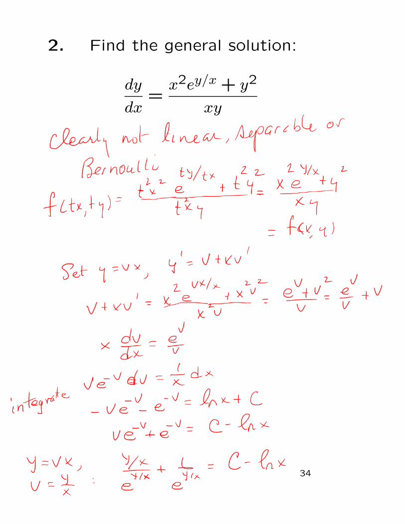
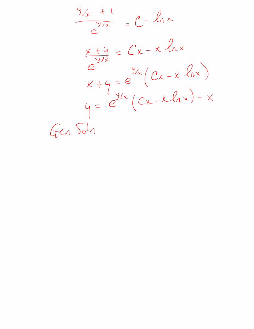
2. Find the general solution:
dy
dx=
x2ey/x + y2
xy
34
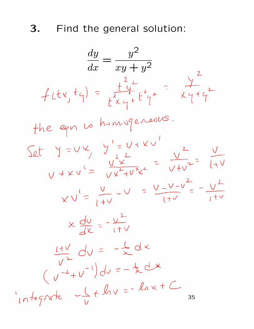
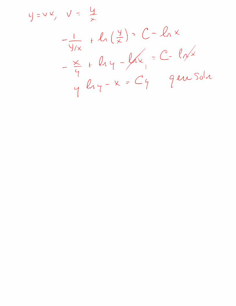
3. Find the general solution:
dy
dx=
y2
xy + y2
35
Top Related