


Languages
Pages
Legal

272
Chapter 12
Local Weak Property Realism: Consistent Histories
Earlier, we surmised that weak property realism can escape the strictures of Bell’s
theorem and KS. In this chapter, we look at an interpretation of quantum mechanics that
does just that, namely, the Consistent Histories Interpretation (CH).
12.1 Consistent Histories
The basic idea behind CH is that quantum mechanics is a stochastic theory
operating on quantum histories. A history a is a temporal sequence of properties held by
a system. For example, if we just consider spin, for an electron a history could be as
follows: at
t0,
Sz = 1; at
t1,
Sx =1; at
t2,
Sy = -1, where spin components are measured in
units of
h /2. The crucial point is that in this interpretation the electron is taken to exist
independently of us and to have such spin components at such times, while in the
standard view 1, 1, and
-1 are just experimental return values. In other words, while the
standard interpretation tries to provide the probability that such returns would be obtained
upon measurement, CH provides the probability Pr(a) that the system will have history a,
that is, such and such properties at different times. Hence, CH adopts non-contextual
property realism (albeit of the weak sort) and dethrones measurement from the pivotal
position it occupies in the orthodox interpretation. To see how CH works, we need first
to look at some of the formal features of probability.
12.2 Probability
Probability is defined on a sample space S, the set of all the mutually exclusive
outcomes of a state of affairs; each element e of S is a sample point to which one assigns
a number
Pr(e) satisfying the axioms of probability (of which more later). An event is a
273
set of one or more sample points (a subset of S). If S contains n elements, then the set of
all events, the event algebra, has
2n elements, including the empty set
Æ (the set with no
points) and S itself. In other words, the event algebra is the set of all the subsets of S.
Given an event A,
~ A is the complement of A, namely, the event of all the points in S
that do not belong to A, that is, the event that occurs if and only if A does not occur.
EXAMPLE 12.2.1
Consider the tossing of a fair die. Then,
S = 1,2,3,4,5,6{ };
1{ } is the event ‘1
appears on top’ and it has probability 1/6;
3,5{ } is the event ‘3 and 5 (in whatever order)
appear on top on two successive tosses’ and it has probability 1/18; S is, for example, the
event ‘a number appears on top’ and
Æ{ } is, for example, the event ‘no number appears
on top.’ Finally, if
A = 3,5{ }, then
~ A = 1,2,4,6{ }.
Given the sample space S and two events A and B on S, one can define two
operations, disjunction and conjunction, as follows.
C = A È B, (12.2.1)
the disjunction of A and B, is the event of all the points that belong to A and/or B. For
example, if
A = 3,5{ } and
B = 1,5{ }, then
C = 1,3,5{ }. C occurs if and only if A and/or B
occurs.
D = A Ç B , (12.2.2)
the conjunction of A and B, is the event of all the points belonging to both A and B. D
occurs if and only if both A and B occur. Disjunction and conjunction satisfy the
following laws L1-L4:
L1, or Commutative Law:
A È B = B È A and
A Ç B = B Ç A .
L2, or Associative Law:
A È B È C( )= A È B( )È C and
A Ç B Ç C( )= A Ç B( )Ç C .
274
L3, or Distributive Law:
A È B Ç C( )= A È B( )Ç A È B( ) and
A Ç B È C( )= A Ç B( )È A Ç B( ).
L4, or Identity Law: there exist two events
Æ{ } and S such that
A È Æ{ }= A and
A Ç S = A .
Any structure on which one can define disjunction, conjunction, and complement in such
a way as to satisfy L1-L4 is a Boolean algebra. Many common algebras such as set
theory and propositional logic, are Boolean algebras. What we are going to do now is to
construct a Boolean algebra in Hilbert space.
EXAMPLE 12.2.2
Suppose we toss two fair dice simultaneously. Then,
3È 5 , (3 or 5 come up),
obtains just in case any, or all, of those numbers comes up.1 By contrast,
1Ç 4 (1 and 4
come up) is true just in case both 1 and 4 come up. Note that
3È 4 says exactly the same
thing as (is equivalent to)
~ ~ 3Ç ~ 4( ), that is, it is false that neither 3 nor 4 come up.
12.3 Properties at a Time
Given a Hilbert space H, assumed to be finite, a projector P identifies a linear
subspace
P of H composed of all and only the eigenkets
c of P such that
P c = c .2
Hence, the generic projector
P = y y operates on the eigenkets in
P as the identity
operator:
P y = y y y = y . When
P = H , then P is the identity operator I that
transforms every ket in H into intself. If
y1,...,yn{ } is an orthonormal basis of H, then
I = yi y i
i
å . (12.3.1)
1 Since
3È 5obtains if and only if ‘
3È 5’ is true, we use the two interchangeably.
2 Here, as in the remainder of this exposition of CH, we follow Griffiths, R., (2002).

275
Clearly, if
f is orthogonal to the members of
P , then it is an eigenket of P but it does
not belong to
P because
P f = y y f = 0. Given a projector P,
~ P = I - P (12.3.2)
is P’s complement.
A physical property is something that can be predicated of a physical system at a
time. For example, ‘the z-component of spin is 1’ is a physical property. Note that a
physical property is always associated with a value. So,
Sz is not a physical property, but
Sz = 1 is. If a system S is described by a ket
c in
P (that is,
P c = c ), then one can
say that S has the property P standardly associated with
c .3 If
c is orthogonal to the
kets in
P (that is,
P c = 0), then S has ~P (the negation of the property P), namely, the
property associated with the projector ~P. If
c is not an eigenket of P, then the
property P is undefined. It follows that a property associated with I always holds and one
associated with the subspace made up of the zero vector never holds. Two projectors P
and Q are orthogonal if
3 Here we denote both the property and its projector as P. Of course, they are not the
same thing: properties exist in the real world, while projectors are abstract entities
existing in configuration space. However, since for simplicity we assume that there is no
degeneracy, there is a one-one correspondence between properties and projectors. At
times, however, we shall denote with
P[ ] the projector associated with property P.

276
PQ = QP = 0.4 (12.3.3)
A decomposition of the identity operator I is a collection of orthogonal projectors
Ri such
that
I = Ri
i
å . (12.3.4)
We can logically link properties by using the following two connectives. The first
connective is conjunction, symbolized by ‘
Ç ’, which stands for ‘and’, so that ‘
P Ç Q’
means P and Q. Rule Q1 says that quantum-mechanically this is represented by
P[ ]× Q[ ],
where
P[ ] is the projector associated with P and
Q[ ] that associated with Q.
The second connective is disjunction, symbolized by ‘
È ’, which stands for
‘and/or’, so that ‘
P È Q’ means P and/or Q. Rule Q2 says that quantum-mechanically
disjunction is represented by
P[ ]+ Q[ ]- P[ ]× Q[ ]. Crucially,
P Ç Q and
P È Q are
defined only if
P[ ] and
Q[ ] commute. It can be shown that a decomposition of the
identity projector I constitutes a sample space and that the event algebra is a Boolean
algebra under the operations of conjunction and disjunction. All of this looks confusing,
but, as the following example will show, there is really less than meets the eye.
EXAMPLE 12.3.1
Consider a spin-half particle in space H. The identity projector on H is
I = + ¯ ¯ , the sum of orthogonal, and therefore commuting, projectors. Consider
now the projector
P = . Then,
P = and the property P is
Sz = 1. If the particle is
4 One must not confuse the orthogonality between vectors (their inner product is zero)
and between projectors (their product is zero). Obviously, orthogonal projectors
commute.

277
in state
, then we can say that it has the property
Sz = 1. If the particle is in state
¯ ,
which is orthogonal to
, then it has the negation of
Sz = 1, namely,
Sz = -1. The
reason is that
I - P = + ¯ ¯ - = ¯ ¯ =~ P and
Sz = -1 is associated with
¯ .
If the particle is in state
1
2 + ¯( ), then
Sz = 1 is undefined. The property associated
with I is ‘
Sz = 1 or
Sz = -1’ and it always hold, while the property ‘
Sz = 1 and
Sz = -1’
never does. The properties ‘
Sz =1( )Ç Sx =1( )’ and ‘
Sz =1( )È Sx =1( )’ are undefined.5
Now let us suppose that particle a is in spin-state
, that it moves, and that its position at
x corresponds to the state
x . Using obvious notation, Q1 says that the quantum
mechanical representation of ‘
Sz =1Ç x =1’ is
( ) 1 1( ), since the two operators
commute. Moreover, Q2 says that the quantum mechanical representations for
‘
Sz =1È x =1’ is
+ 1 1 - ( ) 1 1( ).
12.4 Non-existent Properties
Although CH allows a realist understanding of quantum mechanics, it does not
follow EPR in attributing quantum mechanically incompatible properties to a system.
Griffiths gives an instructive story about what happens if one insists that
P Ç Q is
defined even if P and Q are incompatible. Consider a spin-half particle, and to simplify
the notation, let
Z +[ ] stand for the projector associated with
Sz = 1, and similarly for
other projectors. Suppose now that the composite property
Sz = 1Ç Sx =1 existed. Then
its corresponding projector would have to project onto a subspace
P of the two-
dimensional Hilbert space H of the spin-half particle. However, no such subspace can
exist. For, no one-dimensional subspace
i is associated with both
Sz = 1 and
Sx =1; all
5 In order to avoid clutter, in the future we shall omit the brackets when possible.
278
the one-dimensional subspaces are, as it were, already taken. This leaves only two
subspaces, namely, H itself and the zero-dimensional subspace
0 containing only the zero
vector. Since neither
Sz = 1 nor
Sx =1 are always true,
P ¹ H . If
P = 0, then
Sz = 1Ç Sx =1 (12.4.1)
could never be true, and consequently
Sz =1Ç Sx = -1 (12.4.2)
could never be true as well. Since the disjunction of two false sentences is false,
Sz =1Ç Sx =1( )È Sz =1Ç Sx = -1( ) (12.4.3)
is false as well. Now (12.4.3) is logically equivalent to
Sz = 1Ç Sx = 1È Sx = -1( ) (12.4.4)
which must, therefore, be always false. However, the part in brackets is always true
because the corresponding projector is the identity projector I in H, and consequently
Sz = 1 must always be false. But this cannot be right because at times
Sz = 1 is true. If
we assume that the Hilbert space H contains all the information about the particle, that is,
if we assume that quantum mechanics is complete, then
Sz = 1Ç Sx =1 cannot be assigned
any meaning at all because nothing in H can be associated with it. Moreover, since
conjunction can be defined in terms of disjunction plus negation and vice versa,
Sz = 1È Sx =1 is meaningless as well. In sum, the penalty for logically connecting non-
commuting properties is loss of meaning.
The commuting requirement has interesting consequences for the measurement
problem. As we saw earlier, the measurement problem consists in the fact that according
to TDSE the outcome of measurement is a superposition like

279
¢ Y = c i y i Ä c i
i
å , (12.4.5)
where
y i and
c i are eigenstates of the observed system and the measuring device
respectively. However, we should note that
¢ Y ¢ Y does not commute with any
c i c i , and consequently once
¢ Y ¢ Y obtains it is meaningless to ask whether any of
the
c i c i , or any disjunction of the
c i c i , obtain. In other words, once the
combination atom-Geiger counter-hammer-cyanide container-cat has reached the
measurement superposition TDSE entails, it makes no sense to ask whether the cat is
alive or dead, or even to say that the cat is alive or dead.
12.5 Quantum Histories
Consider a system S and its configuration space H. A history a is a tensor product
of projectors of H such that
a = P1[ ]Ä ... Ä Pn[ ], (12.5.1)
where
Pi[ ] is the projector associated with the property
Pi. History a is itself a projector
in the history Hilbert space
( H = H1 Ä ... Ä Hn , where Hj is S’s configuration space at time
t j . Intuitively, a says that S holds properties P1,…,Pn at times
t1,...,tn . As a sample
space for properties at one time is a decomposition of I, the identity projector for H, into
mutually orthogonal property projectors, so a sample space for histories is a
decomposition of
( I , the identity projector for
( H , into mutually orthogonal history
projectors, so that
a =( I
a
å . (12.5.2)
The rules for negation, conjunction, and disjunction for histories are the same as those for
properties at a single time. Hence, given two histories a and b,
280
~ a =( I - a
aÇ b = ab
aÈ b = a + b - ab.
(12.5.3)
As before, conjunction and disjunction are defined only if a and b commute, that is, only
if
ab = ba. Typically, a and b commute only if all of their component projectors
associated with the same time commute; however, if the two histories are orthogonal
(
ab = ba = 0), then they commute even if not all of their component projectors associated
with the same time commute. The histories that are sample points are elementary
histories, while their combinations in terms of conjunction, disjunction, and negation
(events of more than one sample point) are compound histories. Since they are
orthogonal, elementary histories are mutually exclusive, and therefore they differ from
each other by at least one property projector. The event algebra is a Boolean algebra
under the operations of conjunction and disjunction.
EXAMPLE 12.4.1
Let
a = X +[ ]Ä Z +[ ]Ä Y -[ ] and
b = Y +[ ]Ä Z +[ ]Ä X -[ ] be two histories of
the spin-half system S made of one particle.6 Then
aÇ b and
aÈ b are not defined
because a and b do not commute, since the first and third projectors do not commute and
the two histories are not orthogonal.
The chain operator for a history a is
Ca = PnU tn ,tn-1( )Pn-1 × × ×U t1, t0( )P0 , (12.5.4)
where
P0,...,Pn are the property projectors of a and
U ti,t j( ) is the time evolution
6 To avoid clutter, we often dispense with the subscripts when the temporal ordering of
the system’s properties is clear.
281
operator.7 The probability of a history occurring is given by
Pr(a) = Tr CaC+
a( ), (12.5.5)
where
C+a is the adjoint of
Ca .8
EXAMPLE 12.4.2
Let us determine the probability that an electron originally in state
z will have
the history
a = Z +[ ]Ä X +[ ]Ä Y -[ ] if the Hamiltonian is zero. A simple calculation
gives
Y -[ ]= y y =1
2
1 i
-i 1
æ
è ç
ö
ø ÷ ; similarly,
X +[ ]=1
2
1 1
1 1
æ
è ç
ö
ø ÷ , and
Z +[ ]=1 0
0 0
æ
è ç
ö
ø ÷ .
Consequently, the chain history operator is
Ca =1
2
1 i
-i 1
æ
è ç
ö
ø ÷
1
2
1 1
1 1
æ
è ç
ö
ø ÷
1 0
0 0
æ
è ç
ö
ø ÷ =
1
4
1+ i 0
1- i 0
æ
è ç
ö
ø ÷ .
Finally,
7 Notice that the projector corresponding to the earliest time is on the right. Note also
that when the Hamiltonian is zero, the evolution operator becomes the identity operator,
and can therefore be ignored.
8 Actually,
Tr CaC+
a( ) is not the probability, but the weight (the unnormalized probability,
as it were) of a. The general formula is
Pr(a) =Tr CaC
+a( )
Tr P0[ ], where
P0[ ] is the initial
projector of the history. However, since we are dealing only with orthonormal bases and
pure states,
P0[ ]always projects onto a one-dimensional subspace. Hence, its trace is
always equal to one, and therefore we can use the simpler formula. In the literature, there
are several equivalent formulas for history probability. We look at some of them in
exercise 12.5.

282
Pr(a) = Tr1
4
1+ i 0
1- i 0
æ
è ç
ö
ø ÷
1
4
1- i 1+ i
0 0
æ
è ç
ö
ø ÷
é
ë ê
ù
û ú =
1
4 .
The idea now is to think of quantum mechanics as a stochastic or probabilistic theory:
(12.5.5), which is equivalent to Wigner’s formula, is used to assign probabilities to
quantum histories much in the same way in which classical stochastic theories assign
probabilities to sequences of coin tosses or even to a truly indeterministic sequence of
events.9
12.6 Restrictions on Histories
At this point, however, we must make sure that what we introduced in (12.5.5) is
really a probability, that is, it satisfies the appropriate axioms. There are many equivalent
axiomatic formulation of probability. Here is a simple one consisting of three axioms:
1. Positivity:
0 £ Pr(a) ;
2. Additivity: if a and b are any two mutually exclusive events, then
Pr a Úb( )= Pr a( )+ Pr b( );
3. Normalization:
Pr(e) =1e
å , where e is a sample point.
We can show that (12.5.5) satisfies positivity. An operator O is positive just in case the
elements of its main diagonal are positive. However, given any O such that
Oy = j ,
y ˜ O *Oy = j j ³ 0, (12.6.1)
and therefore
˜ O *O is a positive operator, which entails that its trace is positive.
However, it turns out that (12.5.5) does not always satisfy additivity because of
interference effects among histories, and this requires that the Boolean algebras of events
on which (12.5.5) can be applied must be restricted: histories cannot be lumped together
9 For Wigner’s formula, see appendix five.
283
haphazardly if we want them to obey the rules of probability. The restriction amounts to
the elimination of interference effects so that any two mutually exclusive histories can
evolve separately. As a result, probabilities are assigned only to histories belonging to a
family F if
Tr C+aCb( )= 0, (12.6.2)
where a and b are any two different histories belonging to F. In effect, (12.6.2)
guarantees additivity for history probabilities. If, following Griffiths, we define the inner
product for operators as
A,B = Tr A+B( ), (12.6.3)
then a family is consistent if its history chain operators are orthogonal.10
It can also be shown that (12.5.5) satisfies normalization.
EXAMPLE 12.6.1
Let us investigate whether the three spin-half histories with zero Hamiltonian
a = Z +[ ]Ä Y +[ ]Ä X +[ ],
b = Z -[ ]Ä Y +[ ]Ä X -[ ],
c = Z +[ ]Ä Y -[ ]Ä X +[ ]
form a consistent family. Since
Tr ˜ C a*Cc( )¹ 0, and a, b, and c fail to form a consistent
family. Note that the orthogonality of a and c does not entail that their chain operators
are orthogonal as well.
Determining family consistency can be very laborious, especially when it comes
10 For a proof that (12.6.2) entails additivity, see Griffiths, R., (2002): 140. It turns out
that (12.6.2) is a sufficient but not a necessary condition for additivity.

284
to checking the orthogonality of history chain operators. Nevertheless, there are
shortcuts. One is that if two histories have orthogonal first or last property projectors,
then their chain operators are orthogonal as well. Hence, the spin-half family made up of
d = Z +[ ]Ä Y +[ ]Ä X +[ ],
e = Z -[ ]Ä Y +[ ]Ä X +[ ], (12.6.4)
f = Z +[ ]Ä Y -[ ]Ä X -[ ]
is consistent because any two of the histories have orthogonal first or last members. For
example, the first members of d and e are orthogonal since
Z +[ ]× Z -[ ]= 0 .
EXAMPLE 12.6.2
We can use the above shortcut to come up with a family of histories for a simple
measurement. Suppose we shoot a spin-half particle in state
x through a SGZ device
and that the particle goes through positions
l1 and
l2 on its way to the device, eventually
emerging from it in position
l + or
l -. If
l + and
l - are sufficiently far, so that the
wave packets overlap only minimally, then the respective vector states will be effectively
orthogonal, thus representing mutually exclusive alternatives. Hence, we may consider
l + and
l - as ‘pointers’ correlated with the values of
Sz . One can then construct the
following family made up of two histories
a = X +[ ] l1[ ]Ä Z +[ ] l2[ ]Ä Z +[ ] l +[ ]
and
b = X +[ ] l1[ ]Ä Z -[ ] l2[ ]Ä Z -[ ] l -[ ].11
11 Actually, the family is not complete, and one should add
c = I - X +[ ] l1[ ]{ }Ä I Ä I .
However, since we may set
Pr(c) = 0, this history can be discarded without any loss.

285
The two stories are orthogonal because their last members are, and they show the
measurement correlations between z-spin values and particle position.
12.7 The Risks of Joining Families and Boolean Algebras
Typically, families cannot be mixed: jumping from a family to another in the
same description of a physical process is forbidden. This prohibition marks most clearly
the difference between the quantum and the classical world, and therefore we should look
at it a bit more closely. Two elementary histories in the same family are incompatible in
the sense of being mutually exclusive: if one is true, the others must be false. In other
words, the penalty for combining them is logical inconsistency, a statement of the form
AÇ ~ A. This is not peculiar to quantum mechanics; if it is true that that at a given time
the x-component of the spin of an electron or a billiard ball has a certain value, than it is
false that at that same time it has a different value.
However, histories belonging to different families are incompatible in the sense
that their conjunction generates not a logically inconsistent statement but one that is
neither true nor false, that is, a string of symbols that is no statement at all. To put it
differently, the penalty for combining histories from different families is
meaninglessness. The reason is that every consistent family constitutes a Boolean
algebra of history projectors that acquire probabilities only within that algebraic
framework since, properly speaking, any sort of probabilistic reasoning depends on a
sample space. Quantum mechanics is peculiar in that different algebras of histories
cannot be joined unless certain conditions, ultimately arising from the fact that operator
multiplication is not commutative, are satisfied. So, absent such conditions, if a and b
belong to different families, any statement involving both of them has no probability
286
attached to it (no probability can be defined for it) and is therefore meaningless. In sum,
quantum theoretical statements are probabilistic (“true” means ‘having probability one’
and “false” means ‘having probability zero’), and therefore they presuppose a sample
space. However, typically the non-commutative property of operator multiplication
prevents the construction of a single sample space from those of two families unless
certain special conditions are satisfied. It can also be shown that the prohibition against
joining families allows the adoption of non-contextual weak value determinism without
impinging on the KS theorem (Griffiths, R., (2002): ch. 22).
12.8 A Comparison of CH with the Orthodox Interpretation
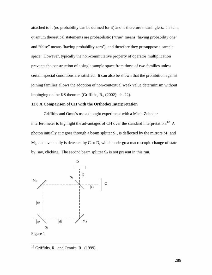
Griffiths and Omnès use a thought experiment with a Mach-Zehnder
interferometer to highlight the advantages of CH over the standard interpretation.12 A
photon initially at a goes through a beam splitter S1, is deflected by the mirrors M1 and
M2, and eventually is detected by C or D, which undergo a macroscopic change of state
by, say, clicking. The second beam splitter S2 is not present in this run.
Figure 1
12 Griffiths, R., and Omnès, R., (1999).
a
d
c
e
f
C
D
S1
S2
M2
M1
287
Using obvious symbolism, the orthodox representation of this story is as follows:
a Ä C Ä D Þ1
2c + d( )Ä C Ä D Þ
1
2C* Ä D + C Ä D*( ) (12.8.1)
where
C* is the state of C clicking, and the arrows indicate the linear temporal
development provided by TDSE. As soon as the system arrives at entanglement between
particle and detector, the state function collapses and one and only one of the two
alternatives is realized. Supposing that the final state of the system is, for example,
C* Ä D , one still cannot know what happened before because of the bizarre
superposition in the intermediate step. In other words, retrodiction from experimental
results is impossible. However, Griffiths and Omnès note, retrodiction is constantly used
by particle physicists, who assume not only that measurements accurately reflect the state
of affairs just before measurement, but even extrapolate which path a particle has
followed before the measurement.
By contrast, CH could employ the two mutually exclusive histories
aCD Ä cCD Ä C*D (12.8.2)
and
aCD Ä dCD Ä CD*, (12.8.3)
to each of which it attributes probability 1/2.13 Here, not only is the collapse postulate
unnecessary, but if the final state of the system is
C*D, we know which history has been
actualized, and therefore we can say that the particle went along path c, with the result
that we need not say, as Griffiths and Omnès flippantly put it, that “experimenters don’t
take enough courses in quantum theory” (Griffiths, R., and Omnès, R., (1999): 29).
13 As before, to avoid clutter, we occasionally write
P instead of
P[ ].

288
It is true that CH also allows histories in which it is meaningless to ask which path
the photon followed, such as
aCD Ä1
2c + d[ ]CD Ä C*D (12.8.4)
and its counterpart in which D clicks. However, one need not use them. Hence, while in
classical physics a single description allows one to answer all the meaningful questions
about a system, largely in quantum mechanics what counts as a meaningful question
depends on the description employed.
Suppose now that we insert a second beam splitter S2 at the intersection of paths c
and d near the detectors C and D, and that we alter the optical path lengths so that S2 will
produce the unitary transitions
c Þ1
2e + f( ) (12.8.5)
and
d Þ1
2- e + f( ), (12.8.6)
with the result that the two
e ’s have opposite phases, and therefore cancel each other
out. The outcome is that all the photons will always travel along f and never along e, so
that D will record hits all the times. At this point, our classical intuitions push us to
wonder whether before getting along f the photon went along c or d. The corresponding
histories are
h = a[ ]Ä c[ ]Ä f[ ] (12.8.7)
and
i = a[ ]Ä d[ ]Ä f[ ]. (12.8.8)

289
Can the two histories be logically connected? For example, can one sensibly ask whether
h È i( )Ç ~ h Ç i( ), that is, the photon went along c or d but not both, or even sensibly
state that
h Ç i, that is, the photon went along both c and d, as one occasionally reads?
According to CH, the answer is negative because the chain operators for the two histories
are not orthogonal, and therefore
h and i cannot belong in the same consistent family.
12.9 The Histories of EPR
In order to discuss the EPR paper with the help of CH, we need to introduce two
notions, that of history extension, and that of support of a family. Moreover, we need to
find out what are the conditions for joining two families into a new family. Suppose that
a = P1 Ä ...Ä Pn and we want to extend a to a time later than
tn . All we need to do is to
set I, the identity operator, for that time:
a = P1 Ä ...Ä Pn Ä In +1. Since I corresponds to a
property that is always true, in effect we have added nothing to our original story,
although, formally, it now extends to a time it did not cover before. The same procedure
applies if the added time is anywhere in the history.
Consider now the histories
a = Z +[ ]Ä Y +[ ]Ä X +[ ], (12.9.1)
and
b = Z +[ ]Ä Y -[ ]Ä X -[ ]. (12.9.2)
Since
a + b ¹( I , they do not constitute a complete family F and that another history c
would have to be added to obtain F. However, it may turn out that they are the only
histories we care about, in which we may set
Pr c( )= 0 and take into account only the
support of F, namely all and only the histories whose probability is greater than zero.
Sometimes, families can be joined. Not surprisingly, two consistent families
290
A = ai{ } and
B = b j{ } are compatible (can be joined) if and only if the following two
conditions are satisfied.
First, the histories belonging to the two families must commute: for all i and j,
ab = ba. This in effect guarantees that a and b can be linked by logical connectives like
aÇ b and
aÈ b. Second, for all a, b, c, d,
Cab ,Ccd = 0 , where
a ¹ c belong to A and
b ¹ d belong to B. In other words, the chain operators of the products of different
histories from the two families must be orthogonal. This condition entails additivity. If
ab = 0 or
cd = 0 (if the histories in the two families are orthogonal), then the second
condition is automatically satisfied.
We can now address EPR by utilizing histories as close as possible to what its
proponents presumably had in mind. Consider, then the family Z with support
Y0Za0 Ä
za+Za
0zb- Ä Za
+zb-
za-Za
0zb+ Ä Za
-zb+
ì í î
, (12.9.3)
where
Za0 is the initial state of an SGZ,
za+ indicates that particle a has the property
Sz = 1,
Za+ indicates that the SGZ has recorded
Sza =1 by absorbing a, and similarly for
the other symbols. Here we have two histories with a common beginning and a split
denoted by the bracket. Note that particles a and b really have the appropriate z-spin
value even before the measurement, and that the measurement correctly correlates the
measurement returns on a with the unmeasured value of z-spin on b, and vice versa.
Consequently, there is no need to appeal to non-locality.
Consider now the family X with support
Y0Xa0 Ä
xa+Xa
0xb- Ä Xa
+xb-
xa-Xa
0xb+ Ä Xa
-xb+
ì í î
, (12.9.4)

291
where the symbols have obvious meaning. To be allowed to say that a and b have both
sharp x-spin and z-spin values, it must be possible for the two families Z and X to be
joined to form a single family for, as we saw, connecting histories from different families
may lead to meaniglessness. In this case, the two families can be joined because the
histories in Z are orthogonal to those in X, since
Y0Xa0( )× Y0Za
0( )= 0 .14 (12.9.5)
However, the joint probability of any history in Z with any history in X is zero, and
therefore EPR was wrong in arguing that a and b have both sharp and opposite x-spin and
z-spin values.
Still, CH seems to intimate that the probability that a and b have both sharp and
opposite x-spin and z-spin values is zero. If so, one might suspect that Einstein lost the
battle but won the war; since only meaningful sentences can have probability zero, one
could infer that Bohr’s position that talk of a particle having simultaneous non-
commuting properties is meaningless is wrong. In other words, does the fact that Z and X
can be joined into a single family ultimately vindicate Einstein’s position that talk of a
particle having simultaneous non-commuting properties makes perfect sense? If so, then
the EPR paper was right in holding that quantum mechanics is incomplete since, as we
saw above, there is no room in Hilbert space for the conjunction of non-commuting
operators.
CH addresses the problem by introducing the notion of dependent event. 14
Xa0[ ] and
Za0[ ] are orthogonal because a SGX and a SGZ differ macroscopically (their
orientations are perpendicular). Since they are multiplied by the same operator, (12.9.5)
holds.

292
Consider the family Z in its entirety. It consists of
Y0Za0 Ä
za+Za
0zb- Ä Za
+zb-
za-Za
0zb+ Ä Za
-zb+
ì í î
, (12.9.6)
namely, the support for Z, and a third history to which we assign probability zero,
namely,
I - Y0Za0( )Ä I Ä I . (12.9.7)
Note that (12.9.7) says nothing at all about the spin components of a and b (I corresponds
to the universal property). Hence Z’s Boolean algebra requires that events
Za+zb
- and
Za-zb
+
be logically dependent on
Y0Za0 (the first event of the only histories in which they
appear) in the sense that one may sensibly ask what is the probability of them obtaining
only in the context of histories beginning with
Y0Za0 . In other words, statements “
Za+zb
-”
and “
Za-zb
+” are meaningful only contextually, given that
Y0Za0 obtains. Similarly,
Xa+ xb
-
and
Xa- xb
+ depend on
Y0Xa0. However, since
Y0Za0 and
Y0Xa0 are mutually exclusive, it
follows that “b’s z-spin component has such and such value” and “b’s x-spin component
has such and such value” can be meaningful only in mutually exclusive contexts.15
12.10 A Review of CH
The basic idea behind CH is to consider quantum mechanics a classic stochastic
theory providing the values of the physical properties a system actually has at a given
time or at different times. Compliance with the laws of probability is obtained by the
construction of Boolean algebras culminating in the notion of consistent family. CH lets 15 Of course, in a way this is nothing new: the end of the EPR paper expressly argues
against this move. CH has an interesting treatment of the counterfactuals apparently
involved in the EPR paper; see section 24.2 of Griffiths, R., (2002).

293
one adopt non-contextual weak value determinism while avoiding non-locality, a feat that
Bell’s theorem had rendered doubtful, and it treats collapse as a mere computational
device with no physical counterpart. Hence, measurement is dethroned from the central
position it enjoys in the orthodox interpretation, and therefore all the (for many)
unpalatable appeals to the observer or even to consciousness can be eliminated.
CH allows great flexibility in the description of a system because within the
confines dictated by the consistency requirements the choice of the times and the
properties with which a history deals is arbitrary. This has startling results not only
because not all synchronous quantum histories of a system can be consistently combined
(a feature present in classical histories as well), but also because synchronous quantum
histories of a system belonging to incompatible families cannot be meaningfully
combined. This entails that, in contrast to a classical system, a quantum one is not
amenable to a single comprehensive description and therefore can be considered from
different and typically non-combinable perspectives. However, the same physical
question will receive the same answer in each different perspective, thus showing that
none is more basic or closer to reality than any other.
It may prove helpful to think about CH in terms of the debate between Einstein
and Bohr. CH partially agrees with Einstein in adopting property realism, albeit in a
weakened form, and rejecting non-locality. However, contrary to the EPR paper, CH
limits our ability to talk about a system by restricting it to consistent families, and with
Bohr treats the attribution of non-commuting properties to a system as meaningless. In a
way, CH can be seen as close to Bohr’s views, for one might think of the idea of
consistent families and their relations as a refinement of Bohr’s idea of complementarity.
294
Nevertheless, in agreement with Einstein, CH dethrones measurement and the role of the
observer from the central position they enjoy in standard quantum mechanics. True, what
family one chooses in the description of a system is up to the physicist, but this is not
different from the fact that in a photograph the point of view is up to the photographer.
What is peculiar is that, because operator multiplication is not commutative, not all such
photographs can be combined to produce a unique overall visual representation of the
object.
The flexibility CH allows in choosing histories may seem to generate some
difficulties. For example, a history in which the projector corresponding to (12.4.5)
occurs, that is, a history in which Schrödinger’s cat appears, although not forced on us, is
still permissible. But, one might object, presumably one would want to have such a
history forbidden. For if superposition has a physical counterpart, while one might
swallow its application to a quantum particle, as in the CH equivalent of (12.8.1), one is
unlikely to do the same with respect to a macroscopic object like a cat. However, as we
saw, for CH the cat is neither dead nor alive, nor dead and alive; indeed, as this applies to
any cat-property one might want to associate with
c i c i in (12.4.5), it turns out that
such a history has times when it cannot say anything about the cat. That is, in such
history, at times when superposition occurs, any talk about the cat’s properties is mere
nonsense, and therefore a fortiori nothing funny is said about the cat.16 This, however,
seems to introduce a further difficulty, namely that in such a history there are times when
the cat seems to vanish, as it were. But the cat, we should remember, is a macroscopic
object: surely, one might insist following Einstein and Shrödinger, in any sensible
16 I owe this point to an exchange with R. B. Griffiths.

295
description of the world Trickster must be in the box at all times with all its proper feline
properties.
A related problem has to do with the fact that there is, at least at the macroscopic
level, only one history, only one actual sequence of events, even if, of course, there are
many possible histories. But CH cannot tell us which history is real, and which is, as it
were, just a historical fable. True, to each history CH associates a probability, but even
so, the theory is unable to tell us which shall emerge into reality. However, this criticism
seems too harsh. After all, for CH the sequence of events in a history is, at least
epistemologically, stochastic, which intimates that the selection of the actual history is, at
least epistemologically, random. If so, it is unreasonable to expect CH to tell us more
than the probability of each history and determine the causal chain, if it exists at all, that
actualized one history rather than another. Even at the macroscopic level, because of the
complexity of the causes involved, the best one can do is to provide probabilities when it
comes to the histories of roulette’s outcomes, leaving aside the issue of what caused one
outcome rather than another.
296
Exercises
Exercise 12.1
Consider a fair coin tossed three times in a row. Determine the sample space. How many
elements will the event algebra have?
Exercise 12.2
What is
3Ç 4 equivalent to, in terms of disjunction and negation? [Hint. Look at
example 12.2.2]
Exercise 12.3
Using rules Q1 and Q2, show that the following equalities hold: a:
P Ç Q = QÇ P ; b:
P È Q Ç R( )= P È Q( )Ç P È R( ).
Exercise 12.4
Do
a = X +[ ]Ä Z -[ ]Ä Y -[ ] and
b = Y +[ ]Ä Z +[ ]Ä X -[ ] commute?
Exercise 12.5
1. Show that (12.5.5) can be written as
Pr(a) = Tr CarCa+( ). [Hint. Look at the rightmost
factor in
Ca . Then, remember that a projector is identical to its square.]
2. Show that (12.5.5) can be written as
Pr(a) = Y Ca+Ca Y . [Hint. Start with the result
of the previous exercise, cyclically rotate the argument of the trace operator, and then
remember what
Tr rA( )is equal to.]
3. Prove that when the Hamiltonian is zero (and the system is conservative) the
evolution operator becomes the identity operator.
4. Verify that in the example above the history probability we got agrees with the
orthodox interpretation concerning the probability of obtaining 1, 1, and
-1 were one

297
to perform the appropriate measurements in succession.
5. Is (4) true in general? [Hint. It turns out that
Pr(a) = Tr CaCa+( )= Tr
) C a
) C a
+( ), where
) C a =
) P n
) P n-1 × × ×
) P 0 , the product of the Heisenberg operators corresponding to the
Schrödinger operators in (12.5.4), and this opens the way for the use of Wigner’s
formula. See appendix 4].
Exercise 12.6
In example 12.6.1 , show that
1. a and c are orthogonal.
2.
Ca,Cb = 0.
3.
Ca,Cc ¹ 0 .
Exercise 12.7
Show that if two histories a and b have orthogonal first or last projectors, then they are
orthogonal.
Exercise 12.8
Show that the chain operators for
h (12.8.7) and
i (12.8.8) are not orthogonal. [Hint.
Notice that the Hamiltonian is not zero, and therefore we use the evolution operators that
need to be applied on density operators represented as ket-bra.]
298
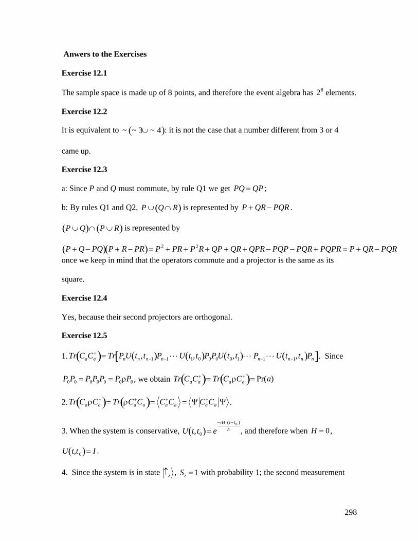
Anwers to the Exercises
Exercise 12.1
The sample space is made up of 8 points, and therefore the event algebra has
28 elements.
Exercise 12.2
It is equivalent to
~ ~ 3È ~ 4( ): it is not the case that a number different from 3 or 4
came up.
Exercise 12.3
a: Since P and Q must commute, by rule Q1 we get
PQ = QP ;
b: By rules Q1 and Q2,
P È Q Ç R( ) is represented by
P + QR - PQR .
P È Q( )Ç P È R( ) is represented by
P + Q - PQ( ) P + R - PR( )= P 2 + PR + P 2R + QP + QR + QPR - PQP - PQR + PQPR = P + QR - PQR
once we keep in mind that the operators commute and a projector is the same as its
square.
Exercise 12.4
Yes, because their second projectors are orthogonal.
Exercise 12.5
1.
Tr CaCa+( )= Tr PnU tn ,tn-1( )Pn-1 × × ×U t1,t0( )P0P0U t0,t1( )× × × Pn-1 × × ×U tn-1,tn( )Pn[ ]. Since
P0P0 = P0P0P0 = P0rP0 , we obtain
Tr CaCa+( )= Tr CarCa
+( )= Pr(a)
2.
Tr CarCa+( )= Tr rCa
+Ca( )= Ca+Ca = Y Ca
+Ca Y .
3. When the system is conservative,
U t,t0( )= e-iH ×(t- t0 )
h , and therefore when
H = 0 ,
U t,t 0( )= I .
4. Since the system is in state
z ,
Sz = 1 with probability 1; the second measurement

299
will return
Sx =1 with probability 1/2 and the state vector will collapse on
x ; the third
measurement will return
Sy = -1 with probability 1/2. Hence, the probability of
obtaining the three returns is
1´1
2´
1
2=
1
4.
5. Yes, because
Tr) C a
) C a
+( )= Tr) C ar
) C a
+( ) is Wigner’s formula.
Exercise 12.6
1. a and c are orthogonal because their second members are.
2.
Cb = X -[ ] Y +[ ] Z -[ ]. Hence,
Ca,Cb = Tr Ca+Cb( )= Tr Z +[ ] Y +[ ] X +[ ] X -[ ] Y +[ ] Z -[ ]( )= 0 .
3.
Ca,Cc = Tr Ca+Cc( )= Tr Z +[ ] Y +[ ] X +[ ] X +[ ] Y -[ ] Z +[ ]( )
= Tr Z +[ ] Y +[ ] X +[ ] Y -[ ]( )¹ 0 .
Exercise 12.7
Let
Ca = PnU tn ,tn-1( )Pn-1 × × ×U t1, t0( )P0 and
Cb = QnU tn , tn-1( )Qn-1 × × ×U t1, t0( )Q0. Then,
Tr Ca+Cb( )= Tr P0U t0,t1( )× × × Pn-1U tn-1,tn( )PnQnU tn,tn-1( )Qn-1 × × ×U t1,t0( )Q0[ ]. Hence, if
PnQn = 0 the result is immediate; if
Q0P0 = 0 the result is obtained by cyclical rotation.
Exercise 12.8
Ch = f f U t3,t2( )c c U t2, t1( ) a a , and
Ci = f f U t3,t2( ) d d U t2, t1( ) a a . Hence,
Tr Ch+Ci( )= Tr a a U t1,t2( )c c U t2,t3( ) f f f f U t3,t2( ) d d U t2,t1( ) a a[ ]. Since
U t2,t1( ) a a =1
2c + d( ) a , after a little algebra we get
Tr Ch+Ci( )=
1
2d c Tr a a U t1,t2( )c c U t2,t3( ) f f f f U t3,t2( ) d a[ ]. Continuing

300
in the same way, we finally obtain
Tr Ch+Ci( )=
1
2d c c d ¹ 0, and therefore the two
chain operators are not orthogonal.
Top Related