


Languages
Pages
Legal


cef.up working paper
2014-02
FINANCIAL SHOCKS AND OPTIMAL MONETARY
POLICY RULES
Fabio Verona Manuel M. F. Martins
Inês Drumond

Financial Shocks and Optimal Monetary Policy Rules∗
Fabio Verona† Manuel M. F. Martins‡ Inês Drumond§
July 25, 2014
Abstract
We assess the performance of optimal Taylor-type interest rate rules, with and without reaction to financial
variables, in stabilizing the macroeconomy following financial shocks. We use a DSGE model that comprises
both a loan and a bond market, which best suits the contemporary structure of the U.S. financial system and
allows for a wide set of financial shocks and transmission mechanisms. Overall, we find that targeting financial
stability – in particular credit growth, but in some cases also financial spreads and asset prices – improves
macroeconomic stabilization. The specific policy implications depend on the policy regime, and on the origin
and the persistence of the financial shock.
Keywords: financial shocks, optimal monetary policy, Taylor rules, DSGE models, bond market, loan market
JEL codes: E32, E44, E52
∗ We thank Efrem Castelnuovo, Jean-Bernard Chatelain, Paolo Gelain, Caterina Mendicino, Jean-Christophe Poutineau, GiuliaRivolta and Margarita Rubio for useful comments and suggestions. During this research, CEF.UP has been financed by PortuguesePublic Funds through FCT (Fundação para a Ciência e a Tecnologia) in the framework of the project PEst-OE/EGE/UI4105/2014.The views expressed are those of the authors and do not necessarily reflect those of the Bank of Finland, the Banco de Portugal or theEurosystem.† Bank of Finland, Monetary Policy and Research Department, and University of Porto, CEF.UP ([email protected])‡ University of Porto, Faculty of Economics and CEF.UP ([email protected])§ Banco de Portugal, Financial Stability Department, and University of Porto, CEF.UP ([email protected])

1 Introduction
The 2007 crisis and the events that followed raised a number of lessons for macroeconomic modeling and for the
strategy of monetary policy (Mishkin, 2011). In this paper we jointly address the implications of three of those
lessons: (i) price and output stability do not ensure financial stability, (ii) cleaning up the effects of financial crises
is very costly and (iii) developments in the financial sector have a far greater impact on economic activity than
previously realized.
Lessons (i) and (ii) relate to the design of monetary policy. As output and inflation stability during the Great
Moderation concealed growing economic and financial imbalances that eventually caused the crisis, and as the
Great Recession has been particularly severe and hard to reverse, the debate on whether monetary policy should
also target financial stability has been reignited (see e.g. Blanchard, Dell’Ariccia, and Mauro 2013). While the
pre-crisis consensus on a dual central bank mandate to stabilise output and inflation still prevails (see e.g. Bernanke,
2013), the case for including a measure of financial vulnerability in the monetary policy reaction function has grown
stronger (see e.g. Borio, 2014b and Stein, 2014), and it has even been argued that a third mandate may eventually
be needed (Reis, 2013). One crucial open issue is what specific measure of financial stability should be targeted,
with suggestions spanning through financial sector or overall leverage, credit or bond spreads, asset (house) prices
and overall credit (see e.g., Woodford, 2012, Gilchrist and Zakrajsek, 2012b, Borio, 2014a and the references in
subsection 1.1).
Lesson (iii) relates to macroeconomic modeling, and encompasses the potential role of financial factors in the
generation of shocks and their propagation to the aggregate economy. In recent years, economists embedded
financial frictions into general equilibrium models, acknowledging that such frictions are crucial in macroeconomic
analysis. There are three main traditions in the literature. One augments the workhorse New Keynesian Dynamic
Stochastic General Equilibrium (NK DSGE) model of Smets and Wouters (2003) with a perfect competition banking
sector that lends to entrepreneurs as a function of their leverage (e.g. Christiano, Motto, and Rostagno, 2014).
Another enhances the model with monopolistic competition in the banking sector (e.g. Gerali, Neri, Sessa, and
Signoretti, 2010). The third introduces financial frictions into the baseline NK DSGE model of Woodford (2003)
with patient and impatient agents, rather than formally modeling a financial sector (e.g. Iacoviello, 2005 and Curdia
and Woodford, 2010). Regarding generation of shocks, the literature has shown that financial shocks – the excess
bond premium shock in Gilchrist and Zakrajsek (2012a), the risk shock in Christiano, Motto, and Rostagno (2014)
or shocks originating in the banking sector in Gerali, Neri, Sessa, and Signoretti (2010) – account for a large share
of business cycle fluctuations, in particular the bulk of recent recessions in the U.S. and euro area.
2
The combined consideration of the lessons (i)-(iii) leads to a research question that compiles three ingredients: how
do monetary policy rules augmented with financial variables perform in an economy featuring financial frictions,
following aggregate fluctuations caused by financial shocks? Such a threefold research programme has not been
thoroughly explored so far, as further reviewed in subsection 1.1 (notable exceptions are Gilchrist and Zakrajsek,
2012b and Davis and Huang, 2013). In the literature featuring the first two ingredients, which dominates the
research field, the performance of monetary policy when the central bank reacts to financial variables depends
largely on the specific model and type of financial friction considered (in addition to the financial variable in the
policy rule). Most importantly, if a common feature of research in the field could be underscored, it would be that
all models consider an economy with only one financial sector and a very limited set of financial frictions and shocks.
However, the U.S. financial system is increasingly composed of two rather different sectors: a traditional banking
system and a non-traditional system, largely non-regulated, highly associated with securitization and harder to
measure – often called the shadow banking system. Most estimates indicate that the latter was larger than the
former in the U.S. economy at the outset of the 2007 crisis, and may still be (see e.g. Pozsar, Adrian, Ashcraft, and
Boesky, 2010 and Gorton and Metrick, 2012). Moreover, it is well-established that non-traditional-bank financial
factors have been particularly relevant in the 2007 financial crisis (see e.g. Akerlof, 2013). So, as Woodford (2010, p.
26) points out, “what is needed is a framework for macroeconomic analysis in which intermediation plays a crucial
role and in which frictions that can impede an efficient supply of credit are allowed for, a framework which also
takes account of the fact that the U.S. financial sector is now largely market-based.”
Hence the motivation for this paper. Using the model previously built by Verona, Martins, and Drumond (2013),
we provide an answer the above stated threefold research question, taking into account the dual composition of
the U.S. financial sector, i.e. the co-existence of a traditional and a non-traditional banking sector. In section 2
we briefly describe the model. Here, we emphasize that our DSGE model features a financial system with a loan
and a bond market and accordingly two different different financial intermediaries – retail and investment banks
– that intermediate financial flows between households (savers) and two groups of entrepreneurs (borrowers) with
different average risk. The retail banking sector is modeled along the lines of the standard Bernanke, Gertler, and
Gilchrist (1999) financial accelerator mechanism, while the bond market is populated by a continuum of monopolistic
competitive investment banks (in the spirit of Gerali, Neri, Sessa, and Signoretti, 2010) that set the coupon rate
on bonds. For realism, we calibrate the model to match the bond-to-bank finance ratio in the U.S. and the cyclical
sensitivity of the spread in bond finance.
The main contributions of the paper are the following. First, we address the relevance of financial stability targets
in the central bank’s policy rule in a model in which a loan and a bond market coexist and which thus features a
3
wider and arguably more realistic set of transmission mechanisms. Second, we assess the performance of alternative
monetary policy rules in reaction to two different financial shocks, one arising in the bond market and one in the
loan market, which affect the cost of borrowing for different entrepreneurs. Third, we seek financial variables that
may improve the ability of monetary policy to stabilize the economy, looking at both segments of the financial
system, the traditional banking sector and the bond market.1
The flavor of our main results can be given in five points. First, an explicit target for financial stability usually
improves the ability of monetary policy to stabilize the aggregate economy. Second, targeting credit growth seems
to be the most effective policy, as compared to other financial indicators (financial spreads and asset prices). Third,
the role of monetary policy appears to be larger following shocks in the bond market than following shocks in the
loan market. Fourth, the case for a monetary policy targeting financial stability increases with the persistence of
the financial shocks that cause the economic fluctuations. Fifth, if the central bank aimed at maximizing social
welfare rather than fulfilling its mandate, policy would respond even more aggressively to financial variables and
less so to inflation.
The rest of the paper is organized as follows. In the next subsection we briefly review the related literature. In
section 2 we present the main distinctive features of our model, and then describe the two financial shocks that are
the source of fluctuations in our simulations. In section 3, we describe the method used to assess the performance
of alternative monetary policy rules, present the results of our simulations, and provide some sensitivity analyses.
Section 4 concludes.
1.1 Related literature
Our paper is closely related to three strands of literature. First, at a more general level, is the literature on the
relation between financial and business cycles, emphasizing how the 2007 crisis reopened the debate on the reaction
of monetary policy to financial (in)stability, changed the perception and measurement of financial disruptions, and
stimulated research that puts financial shocks at the center of business cycles. Second, and more specific, is the
literature that has assessed the performance of monetary policy rules that include reactions to financial variables,
in the context of different DSGE models with financial frictions. Finally, at a more technical level, is the literature
on the concept and implementation of optimal policy, which distinguishes between analyses based on fulfillment of
the central bank mandate and analyses based on social welfare measures.1 It should be stressed that the focus of our paper is to assess whether monetary policy should take into account financial variables
for macroeconomic stabilization purposes. It does not attempt to address the macroprudencial policy role, and, consequently, the recentdebate on establishing the right balance between monetary policy and macroprudencial policy in the pursuit of financial stability.
4
1.1.1 Financial and business cycles: policy, measurement and shocks
Macroeconomists are now well aware that recessions associated with financial disruptions tend to be sharper and
to be followed by slower recoveries than other recessions, as correction of financial imbalances is typically long and
difficult, and the transmission of stimulative policy is hampered by financial rebalancing (Cerra and Saxena, 2008,
Claessens, Kose, and Terrones, 2009, Reinhart and Rogoff, 2009, and Claessens, Kose, and Terrones, 2012). Before
the 2007 crisis, when financial stability was usually defined in terms of deviations of asset prices from fundamentals
(i.e. asset price bubbles), the dominant view was that monetary policy should not lean against asset bubbles, but
rather clean the effects of bubbles once they burst (see e.g. Cecchetti, Genberg, Lipsky, and Wadhwani, 2000 and
Borio and Lowe, 2002). The crisis has now reopened this debate.
On the one hand, the accumulated loss of output has been exceedingly large and policy particularly ineffective in the
wake of massive deleveraging. Consistently, recent research has shown that the ability of monetary policy to induce
recoveries from recessions caused by financial crises is very limited and often insignificant, with deleveraging paying
a more important role (see e.g. Bech, Gambacorta, and Kharroubi, 2014). Hence, while it has been acknowledged
that financial cycles tend to be longer than economic cycles (Borio, 2014a), it has increasingly been argued that
monetary policy should lean more aggressively against financial booms, so that policy would not be overburdened
during busts (see e.g. Borio, 2014b).
On the other hand, it has been realized that more than in asset prices misalignments, the crisis was marked by
excessive credit growth and leverage, associated with too much risk-taking and abnormally narrow spreads. Indeed,
recent research has highlighted the fact that credit is the main predictor of financial crises, at least since the “new
financial era” that began in 1945, characterised by a decoupling of credit from money (Schularick and Taylor, 2012).
In the same vein, Jorda, Schularick, and Taylor (2011) showed that the severity of recessions is systematically related
to the intensity of the build-up of excessive leverage during the preceding expansion, as measured by excessive growth
of credit relative to GDP. Accordingly, credit-driven bubbles came to be considered more important, and easier to
monitor and predict, than asset price bubbles (see e.g. Adrian and Shin, 2010). Hence the modern approach of
defining financial stability in terms of risk, spreads, credit growth and leverage (see e.g. Gertler and Kiyotaki, 2010
and Curdia and Woodford, 2010). Overall, the events following the 2007 crisis as well as the accumulated knowledge
about financial crises, moved the prescription that monetary policy should react to financial booms, and not only
to busts, to the center of discussions in academic and policymaker circles.
At a more theoretical level, the recent events and empirical research led to the suggestion that, in the presence of
financial frictions, financial shocks explain a significant part of the business cycle. Christiano, Motto, and Rostagno
5

(2014) suggest that risk shocks (i.e. fluctuations in the volatility of the idiosyncratic shocks faced by leveraged
entrepreneurs) account for a large share of business cycle fluctuations. Estimating a similar model, Kaihatsu and
Kurozumi (2014) show that for both Japan and the U.S. financial shocks are at least as important for investment
fluctuations as technology shocks, and that favorable and subsequent unfavorable shocks to the external finance
premium induced the boom and bust cycles of investment during the late 1980s and the 1990s in Japan and since
2004 in the U.S. With a similar model, but using the excess bond premium suggested by Gilchrist and Zakrajsek
(2012a) as the measure of financial distress (a component of the corporate bond spread that measures the pricing
of overall default risk), Gilchrist and Zakrajsek (2011, 2012b) find that changes in such a measure of financial stress
cause changes in credit spreads that transmit to the aggregate economy, explaining the bulk of recent U.S. recessions
as well as the investment booms of 1995-2000 and 2003-06.
1.1.2 Monetary policy and financial (in)stability: models and results
Given the renewed interest in the reaction of monetary policy to financial (in)stability, several papers in recent
years have assessed the performance of monetary policy rules augmented with financial variables. Whereas asset
prices dominated this literature in its earlier stages, financial measures such as spreads and credit have gradually
gained in importance, in line with the course of events described in 1.1.1. Research has essentially been conducted
in the context of three main classes of DSGE models with financial frictions.
First, the Smets and Wouters (2003) NK DSGE model augmented with a perfect competition banking sector and
a Townsend (1979) debt contract (with the resulting Bernanke, Gertler, and Gilchrist, 1999 financial accelerator
effects). With such a model, Faia and Monacelli (2007) find that the policy interest rate should not react significantly
to asset prices, as the gains in output and inflation stabilization would be negligible. More recently, Gilchrist and
Zakrajsek (2012b) and de Fiore and Tristani (2013) find that augmenting the monetary policy rule with a reaction
to credit spreads effectively dampens the effects of financial disruptions, with gains in macro stabilization. Yet
more recently, Davis and Huang (2013) find that as credit frictions or risk shocks become more severe (and the
output-inflation tradeoff less favorable), inclusion of the credit spread in the central bank policy rule (even with
no explicit target for financial stability in the central bank’s loss function) results in a policy closer to its optimal
path, with lower volatility of both output and inflation.
Secondly, models that introduce financial frictions in the NK DSGE model of Woodford (2003) without a formal
financial sector. Iacoviello (2005) develops a model with patient and impatient households, as well as entrepreneurs,
in which there are collateral constraints tied to housing values on both the firm and the household side, finding
6
that a response of monetary policy to asset prices does not yield significant gains in terms of output and inflation
stabilization. Curdia and Woodford (2010) consider a time-varying spread (wedge) between the interest rate re-
ceived by patient households (lenders) and the interest rate payed by impatient households (borrowers), and find
that adjusting the standard Taylor rule for variations in credit spreads improves welfare, with the magnitude of the
adjustment depending on the source and persistence of shocks. Nistico (2012) considers an economy with hetero-
geneity in households related to the accumulated stock of financial wealth, and a financial friction caused by the
interplay between households with and without wealth, finding that policy reactions to deviations in the stock-price
growth rate may imply substantial stability gains.
Third, the Smets and Wouters (2003) model augmented with a monopolistically competitive banking sector, as in
Gerali, Neri, Sessa, and Signoretti (2010), where the banks’ loan margins depend on their capital-to-assets ratio.
Such a model adds frictions on the side of lenders (bank lending channel) to the Iacoviello (2005) collateral channel
on the side of borrowers. Using this model, Gambacorta and Signoretti (2014) find that augmenting a Taylor-type
policy rule with a target for credit and, even more so, for asset prices, improves output and inflation stabilization
under supply shocks, with the stabilization gains increasing with the degree of leverage in the economy. Hirakata,
Sudo, and Ueda (2013) develop a model with interest rate spreads between lenders, financial intermediaries and
borrowers that depend on entrepreneurs’ and financial intermediaries’ net worth, and find that in many cases
(depending on the nature of shocks and the specific financial spread considered) spread-adjusted rules dominate
simple Taylor-type rules.
1.1.3 Optimal monetary policy: central bank’s mandate vs social welfare
As regards the concept and implementation of optimal monetary policy, there are two main traditions in the
literature. One follows Woodford (2003) and studies the social welfare-maximizing policy, i.e. the policy that
maximizes (a second order approximation to) the households’ utility function (see e.g. Faia and Monacelli, 2007,
Kobayashi, 2008, Curdia and Woodford, 2010, Gertler and Karadi, 2011, Woodford, 2012, de Fiore and Tristani,
2013, Hirakata, Sudo, and Ueda, 2013, Lambertini, Mendicino, and Punzi, 2013 and Quint and Rabanal, 2014).
The other considers that the optimal policy is the one that best achieves the central bank’s mandate, i.e. that
intertemporally minimizes the central bank’s loss function, usually defined as the weighted sum of the variances of
inflation, output gap and of nominal interest rate changes (see e.g. Castelnuovo and Surico, 2004, Dieppe, Kuster,
and McAdam, 2005, Jung, Teranishi, and Watanabe, 2005, Lippi and Neri, 2007, Sala, Soderstrom, and Trigari,
2008, Adolfson, Laseen, Linde, and Svensson, 2011, Nistico, 2012, Davis and Huang, 2013, and Gelain, Lansing,
and Mendicino, 2013).
7

While the first approach has the advantage of allowing for theory-consistent Ramsey policy and analytical social
welfare analyses, it has several disadvantages. In particular, it is more complex, less robust, not necessarily imple-
mentable, difficult to verify, and sensitive to all distortions in the economy (Adolfson, Laseen, Linde, and Svensson,
2011). The latter is especially important in models with financial frictions such as ours, as social welfare surely
depends on the misallocation of resources arising from financial distortions. Moreover, the issue of implementability
is crucial when the objective of the research is to identify augmented policy rules that central banks may actually
pursue and which are beneficial for macroeconomic stabilization. These are the main reasons for our choice of the
second approach as the main approach in this paper. But we also provide additional insights from a welfare analysis
based on numerical approximations.
The simulations presented in section 3 consider alternative financial variables in augmented Taylor-type policy rules
(as in the literature reviewed in 1.1.2) and check their relative performance among the possible set of policy regimes
(those that best mimic the central bank’s mandate, as reviewed in this subsection) when the economy is buffeted
with financial shocks (as some literature reviewed in 1.1.1). Before conducting these simulations, in section 2 we
briefly present the distinctive features of the model, as well as its baseline dynamics following financial shocks.
2 The model
Figure 1 sketches the structure of the model, which follows very closely Verona, Martins, and Drumond (2013). The
economy is composed of households, final- and intermediate-good firms, capital producers, entrepreneurs, banks,
and government. Households consume, save and supply labor services monopolistically. They allocate their savings
between time deposits and corporate bonds.2 On the production side, monopolistically competitive intermediate-
good firms use labor (supplied by households) and capital (rented from entrepreneurs) to produce a continuum
of differentiated intermediate goods. Perfectly competitive final-good firms buy intermediate goods and produce
the final output, which is then converted into consumption, investment and government goods. Capital producers
combine investment goods with undepreciated capital purchased from entrepreneurs to produce new capital, which
is then sold back to entrepreneurs. Entrepreneurs own the stock of physical capital and rent it to intermediate-good
firms. They purchase capital using their own resources as well as external finance (bank loans or bonds issuance).
Government expenditures represent a constant fraction of final output and are financed by lump-sum taxes imposed
on households, with the government budget being systematically balanced. The central bank sets the nominal
interest rate according to a Taylor-type interest rate rule.2 The return on corporate bonds equals the return on time deposits, which in turn is equal to the central bank nominal interest rate.
8
Except for entrepreneurs and financial intermediaries, the model is a standard NK DSGE model in the vein of Smets
and Wouters (2003) and Christiano, Eichenbaum, and Evans (2005). We refer the reader to Verona, Martins, and
Drumond (2012, appendix A) for a detailed description. In what follows, we describe the financial system of the
model.
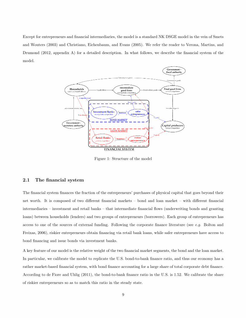
Figure 1: Structure of the model
2.1 The financial system
The financial system finances the fraction of the entrepreneurs’ purchases of physical capital that goes beyond their
net worth. It is composed of two different financial markets – bond and loan market – with different financial
intermediaries – investment and retail banks – that intermediate financial flows (underwriting bonds and granting
loans) between households (lenders) and two groups of entrepreneurs (borrowers). Each group of entrepreneurs has
access to one of the sources of external funding. Following the corporate finance literature (see e.g. Bolton and
Freixas, 2006), riskier entrepreneurs obtain financing via retail bank loans, while safer entrepreneurs have access to
bond financing and issue bonds via investment banks.
A key feature of our model is the relative weight of the two financial market segments, the bond and the loan market.
In particular, we calibrate the model to replicate the U.S. bond-to-bank finance ratio, and thus our economy has a
rather market-based financial system, with bond finance accounting for a large share of total corporate debt finance.
According to de Fiore and Uhlig (2011), the bond-to-bank finance ratio in the U.S. is 1.52. We calibrate the share
of riskier entrepreneurs so as to match this ratio in the steady state.
9

2.1.1 The bond market
The bond market is populated by a continuum of monopolistic competitive investment banks. Each investment bank
has some market power when conducting its intermediation services with safer entrepreneurs, but we assume perfect
competition in the market for households’ deposits. Let εcoupont+1 > 1 be the time-varying interest rate elasticity of
the demand for funds in the bond market. Under the above assumptions, the bond coupon rate Rcoupont+1 is given by
1 +Rcoupont+1 =εcoupont+1
εcoupont+1 − 1
(1 +Ret+1
),
that is, the coupon rate is a time-varying markup,εcoupont+1
εcoupont+1
−1, over the nominal interest rate Ret+1. The spread in
bond finance, i.e. the spread between the bond coupon rate and nominal interest rate is
bond spreadt+1 ≡ Rcoupont+1 −Ret+1 =1
εcoupont+1 − 1
(1 +Ret+1
). (1)
Equation (1) shows that the bond spread is time-varying. In fact, corporate bond spread co-moves with the
business cycle (see e.g. Gilchrist and Zakrajsek, 2012a). To determine the behavior of the bond spread, we specify
the following baseline relation between the elasticity of the demand for funds and the cyclical state of the economy,
summarized by the output gap (i.e. the difference between current output Yt and its steady-state value Y ):
εcoupont+1 = ε+ α1
(Yt − Y
).
As detailed in Verona, Martins, and Drumond (2013), ε is chosen to match the average annual bond spread in the
data, and α1 to match the cyclical sensitivity of the bond spread according to very long historical U.S. time series.
As further detailed in subsection 2.2.1, we define the shock to bond finance as a shock to the elasticity εcoupont+1 . In
particular, a positive shock to this elasticity reduces the markup on the bond rate, the bond coupon rate and the
bond spread.
2.1.2 The loan market
Our modeling of the loan market follows closely Bernanke, Gertler, and Gilchrist (1999) and Christiano, Motto,
and Rostagno (2014). A riskier entrepreneur purchases K units of physical capital, which then turns into ωK units
of effective capital, where ω > 0 is a unit mean, lognormally distributed random variable, drawn independently
by each entrepreneur. The standard deviation of logω is denoted by σt and is assumed to be the realization of a
10

stochastic process.
The realization of ω is observed by the entrepreneurs at no cost, while the retail bank has to incur in a monitoring
cost to observe it. To deal with this problem of asymmetry of information, the entrepreneurs and bank sign a debt
contract, according to which the entrepreneur commits to pay back the loan principal and a non-default interest rate
Z, unless he defaults. In this later case, the bank undertakes a costly verification of the value of the entrepreneur’s
assets and takes in all of the entrepreneur’s net worth. Financial frictions – reflecting the costly state verification
problem between entrepreneurs and the bank – imply that the bank hedges against credit risk by charging a premium
over the riskless nominal interest rate. As shown by Bernanke, Gertler, and Gilchrist (1999), the credit spread (i.e.,
the wedge between the cost of external finance and the risk-free rate) depends positively on the entrepreneur’s
leverage ratio. All else equal, higher leverage means higher exposure, implying a higher probability of default and
thus a higher credit risk, which leads the bank to charge a higher lending rate.
The credit spread also fluctuates with changes in σt. In particular, an increase in idiosyncratic uncertainty raises
the cost of external finance, and so reduces the amount of credit extended to riskier entrepreneurs. With fewer
financial resources, these entrepreneurs acquire less physical capital, and the price of their capital falls. We refer
to σt as the loan market shock, and present details of its modeling in subsection 2.2.2.3
2.2 Financial shocks
The model comprises two financial shocks, one in each of the financial market segments. Both are credit supply
shocks that, when positive, may be thought of as a favorable shock to the financial intermediation process in its
market segment, shifting the respective supply curve to the right. In this subsection, we present our modeling
approach to both shocks and describe the dynamic response of our economy to each shock.
2.2.1 The bond market shock
In the bond market, we assume a shock νt that follows an AR(1) process:
νt = ρννt−1 + σνt .
3 A similar interpretation of this shock is given by de Fiore, Teles, and Tristani (2011), Davis and Huang (2013) and Quint andRabanal (2014). In contrast, Christiano, Motto, and Rostagno (2014) and Chugh (2014) interpret this as a risk shock, since risk ishigh in periods when σt is high, as there is a wider dispersion in capital outcomes across entrepreneurs. Gilchrist and Zakrajsek (2011)model this shock in an alternative way, introducing a direct shock to the effective cost of financial intermediation.
11
The shock influences the elasticity of demand for bonds
εshockt+1 = εcoupont+1 (1 + νt)
and thus the bond coupon rate
1 +Rcoupon,shockt+1 =εshockt+1
εshockt+1 − 1
(1 +Ret+1
)
and the bond spread
bond spreadshockt+1 =1
εshockt+1 − 1
(1 +Ret+1
).
A positive shock to νt increases the elasticity of the demand for bond finance and reduces the markup, the bond
coupon rate and the bond spread. We calibrate the autoregressive coefficient ρν = 0.9 in line with long-run data
for the U.S. financial bond spread. Specifically, our calibration corresponds to the AR(1) regression coefficient of
the difference between (quarterly averages of) the Moody’s Seasoned Baa Corporate Bond yields and the 10-Year
Treasury constant maturity yields, from 1953:I to 2011:IV. We set the size of the shock σνt so that, on impact, the
bond spread decreases by 50 basis points (annual rate).
Blue solid lines in figure 2 are the impulse response functions of selected variables to a favorable bond market shock
(red dashed lines are the impulse response functions to a favorable loan market shock, which will be discussed in
the next subsection). The top panel reports aggregate variables, the middle panel variables relative to the safer
entrepreneurs (who have access to bond finance), and the bottom panel variables relative to the riskier entrepreneurs
(who obtain bank finance).
Following a positive shock to σνt , safer entrepreneurs increase markedly their demand for credit (bonds), as they face
a markedly lower interest rate for a prolonged period of time. The rise in capital purchases by safer entrepreneurs
more than compensates for the increase in their net worth, so their leverage rises noticeably above the steady-state
level.
As regards the riskier entrepreneurs, even though their cost of financing also drops (because of the decline in their
leverage), bank finance is nevertheless more expensive than bond finance (the loan spread falls by around 25 basis
points on impact, while the bond spread falls by 50 basis points), and so riskier entrepreneurs cut their capital
expenditures and the amount of borrowing from retail banks declines considerably.
At the aggregate level, given that safer entrepreneurs represent a larger share of the total population of entrepreneurs,
there is a credit boom driven by the increase in the demand for bond finance. The increase in safer entrepreneurs’
demand for capital pushes up aggregate demand (investment and output) as well as the price of capital, while the
12
decrease in the price of finance leads to a fall in inflation. The central bank, who follows a Taylor-type policy rule
with a strong response to inflation and a weak response to the output gap (see equation 2 below), cuts the nominal
interest rate in response to the fall in inflation.
The bond finance shock, as well as the dynamic responses of the economy, are very persistent (later in the paper
we check the sensitivity of the results to different calibrations of ρν). At the aggregate level, output peaks about 20
quarters after the shock and inflation falls until a few quarters later, the price of capital takes more than 20 quarters
to resume its steady-state level and total credit peaks around 25 quarters after the shock. As regards the variables
related to safer entrepreneurs, the bond spread takes about 40 quarters to resume its steady-state level and both
leverage and bond issuance peak somewhat after 20 quarters but remain above their steady-state levels throughout
the 40-quarter horizon. As regards riskier entrepreneurs, the loan spread, the amount of loans and leverage return
to their steady-state levels by 30 quarters after the shock.
2.2.2 The loan market shock
In the loan market, we consider an AR(1) shock to the standard deviation of the entrepreneur’s idiosyncratic
productivity:
σt = σ (1 − σσt ) + ρε (σt−1 − σ) .
A positive shock to σt reduces the idiosyncratic uncertainty, the credit risk and the loan spread. We calibrate
ρε = 0.722, which is the value estimated by Christiano, Motto, and Rostagno (2010) using aggregate U.S. data.
The size of the shock σσt is chosen so that, on impact, the loan spread, Z−Re, decreases by 50 basis points (annual
rate).
Red dashed lines in figure 2 plot the impulse response functions of selected variables to this shock. Facing a lower
cost of financing, riskier entrepreneurs borrow aggressively and their leverage increases markedly. In contrast to
what happens in the reaction of safer entrepreneurs’ borrowing to a favorable bond shock, the effects of the loan
shock on borrowing and leverage of riskier entrepreneurs is short-lasting, i.e. the financial variables related to the
set of entrepreneurs that use bank finance return swiftly to their steady states (later in the paper we check the
sensitivity of the results to different calibrations of ρε).
Regarding safer entrepreneurs, bond finance becomes relatively more expensive than bank finance, as the bond
spread barely changes and the loan spread takes about 10 quarters to return to its steady-state level, so there is a
large decline in the amount of bonds issued in the economy. Accordingly, their leverage falls markedly for about 10
quarters.
13

At the aggregate level, there is not much action, because of the small weight of riskier entrepreneurs in our market-
based economy (that, recall, aims at resembling the structure of the U.S. financial system). The increase in bank
loans is totally compensated by the decline in bond issuance, even though the magnitude of the former is much
larger than the magnitude of the latter, so that total credit barely changes. Accordingly, the loan market shock plays
virtually no role as a driver of aggregate macro fluctuations: output and investment barely move, while inflation
increases only slightly for a few quarters, which leads to only a tiny reaction of the policy interest rate for a very
limited period after the shock. The neutrality of the loan shock in our model is similar to the findings of Chugh
(2014) for a frictionless real business cycle model augmented with the agency-cost framework of Carlstrom and
Fuerst (1998), but contrasts with the results obtained with NK DSGE models by Christiano, Motto, and Rostagno
(2014) and Gilchrist and Zakrajsek (2011, 2012b). Such contrast is explained by the fact that in these papers the
loan market corresponds to the whole financial system, while in our paper the loan market is smaller than the bond
market.
Having presented the model, the financial shocks and the baseline dynamic responses of our economy to these
shocks, we now move to the core question of our paper: does a reaction of monetary policy to financial variables
improve macroeconomic stabilization in our economy, following financial shocks?
3 Optimal monetary policy rules and financial (in)stability
In order to assess whether a reaction of monetary policy to financial vulnerability improves policy outcomes, one
has to (i) model the reaction of policy, (ii) measure financial vulnerability and (iii) establish a criterion for policy
effectiveness. In what follows we address (i) and (ii). In subsection 3.1 we explain and use our main criterion for
policy evaluation (iii), namely the performance of the policymaker in fulfilling its mandate. Then, in subsection 3.2
we explore an alternative criterion – maximization of social welfare. Finally, subsection 3.3 presents some sensitivity
analyses.
We follow, in our analyses, the standard assumption that monetary policy is effectively modeled with Taylor-type
interest rate rules, considering equation (2) as the benchmark Taylor rule (BTR). It includes interest rate smoothing
and responses of the nominal interest rate to deviations in expected inflation (Etπt+1) and current output from
their steady states:
Ret = ρRet−1 + (1 − ρ)
[Re + φπ (Etπt+1 − π) + φy
(Yt − Y
Y
)], (2)
where Re and π are the steady-state values of Ret and πt, respectively, απ and αy are the weights assigned to
14

expected inflation and output, and ρ captures interest rate smoothing.
The policy outcomes of this benchmark rule will be compared with those of rules augmented with a measure of
financial vulnerability. In this regard, a crucial issue is what specific indicator of financial vulnerability should be
included. The preferred indicator should i) be easy to measure, ii) relate closely to overall economic stability and iii)
be controllable by monetary policy. There is a wide variety of financial indicators in the literature, and the issue is
clearly still open. Taylor rules have been augmented with asset prices (e.g. Faia and Monacelli, 2007), credit-growth
(e.g. Christiano, Motto, and Rostagno, 2010, Gelain, Lansing, and Mendicino, 2013 and Lambertini, Mendicino,
and Punzi, 2013), credit spreads (e.g. Curdia and Woodford, 2010, Merola, 2010, Gilchrist and Zakrajsek, 2011,
2012b, Davis and Huang, 2013, Hirakata, Sudo, and Ueda, 2013 and Stein, 2014), asset prices growth (Nistico, 2012,
Gelain, Lansing, and Mendicino, 2013 and Lambertini, Mendicino, and Punzi, 2013), the level of credit (either the
credit-to-GDP ratio or percentage deviation from steady state, as in Curdia and Woodford, 2010 and Quint and
Rabanal, 2014), and financial sector leverage (Woodford, 2012).
All considered, we assess the performance of Taylor-type rules augmented with four alternative measures of financial
vulnerability: a rule augmented with asset prices (ATR1), which in our model correspond to the price of capital
goods; a rule augmented with credit growth (ATR2), which in our model comprises the total bond issuance and
credit granted; and a rule augmented with credit spreads, split into two sub-rules, one augmented with the bond
spread, (ATR3a), the other augmented with the loan spread (ATR3b).4
• ATR1:
Ret = ρRet−1 + (1 − ρ)
[Re + φπ (Etπt+1 − π) + φy
(Yt − Y
Y
)+ φq
(qt − q
q
)](3)
where qt is the price of capital and q is its steady-state value;
• ATR2:
Ret = ρRet−1 + (1 − ρ)
[Re + φπ (Etπt+1 − π) + φy
(Yt − Y
Y
)+ φ∆credit
(Bt+1 −Bt
Bt
)](4)
where Bt is aggregate credit (the sum of bonds and bank loans);
• ATR3a:
Ret = ρRet−1 + (1 − ρ)
[Re + φπ (Etπt+1 − π) + φy
(Yt − Y
Y
)− φbs
(BSt −BS
)](5)
4 We have also conducted simulations with the growth rate of asset prices, and some measures that capture the level of credit, butthose indicators turned out not to improve economic stabilization in our model.
15

where BSt = Rcoupont − Ret , BS = Rcoupon − Re and Rcoupon is the steady-state value of the bond coupon
rate;
• ATR3b:
Ret = ρRet−1 + (1 − ρ)
[Re + φπ (Etπt+1 − π) + φy
(Yt − Y
Y
)− φls
(LSt − LS
)](6)
where LSt = Zt+1 −Ret , LS = Z−Re and Z is the steady-state value of the contractual interest rate on bank
loans.
3.1 Policymakers’ preferences and optimal rules
In this subsection we compare the performances of rules ATR1, ATR2, ATR3a and ATR3b relative to the baseline
rule (BTR), for an economy hit by financial shocks, using as the assessment criterion the ability of the central
bank to achieve its mandate, i.e. to intertemporally minimize its loss function. The preferences of the policymaker
include a primary goal of price stability and a goal of stabilization of output around potential, which corresponds
to the flexible inflation targeting that characterizes modern central banks (see e.g. Svensson, 2010). There is also
an objective of minimizing the volatility of changes in the policy interest rate, consistent with the fact that central
banks typically feature interest rate smoothing (see e.g. Aguiar and Martins, 2005). Analytically, we assume that
the central bank’s mandate may be described as the objective of minimizing a weighted average of the variances of
inflation, output gap and policy interest rate changes:
Loss Function = απvar (π) + αyvar (y) + +αrvar (∆Re) .
This general loss function (LF) is flexible enough to encompass a wide range of policy regimes, corresponding to
different emphases on price, output and interest rates stability, as a function of the specific weights απ, αy and αr.
In the empirical literature, many studies provide estimates for these weights (see e.g. Lippi and Neri, 2007, Adolfson,
Laseen, Linde, and Svensson, 2011 and Ilbas, 2012). In practice, monetary policy regimes differ considerably across
economies and along time, and so for completeness we conduct our simulations for a set of policymakers’ preferences,
considering three policy regimes and six different parameterizations of their relative weights, as reported in Table
1 (our weights are in line with those often used in the literature, see e.g. Ehrmann and Smets, 2003). The first
policy regime (LF1) is a strict inflation targeting regime, pursued by a central bank that is only concerned with
inflation stability. The second policy regime is one of flexible inflation targeting, in which the central bank also
aims at stabilizing the output gap (here we consider three alternative values for the coefficient attached to output,
16

Loss function απ αy αr
LF1 1 0 0LF2 1 1 0LF3 1 0.5 0LF4 1 0.1 0LF5 1 0.5 0.1LF6 1 0.1 0.1
Table 1: Loss functions and monetary policy regimes
LF2, LF3 and LF4). Finally, LF5 and LF6 are flexible inflation targeting regimes in which the central bank further
aims at reducing the volatility of the nominal policy interest rate.
We conduct two experiments, proceeding in steps towards optimized Taylor-type rules.
In the first experiment, we hold the coefficients in the benchmark Taylor rule at the baseline values, ρ = 0.88,
φπ = 1.82 and φy = 0.11 (as in Verona, Martins, and Drumond, 2013), and allow the coefficients associated with
the financial variable, namely asset prices (φq), credit growth (φ∆credit), loan spread (φbs) and bond spread (φbs)
in (3)-(6), to vary between 0 and 1. Figure 3 plots the value of the loss functions for all policy regimes (LF1-LF6)
in the case of a shock in the bond market, for all possible values of the coefficients associated to φq, φ∆credit, and
φbs in the top, middle and bottom panel respectively. Figure 4 depicts the results of the same exercise for a loan
market shock (there, the bottom panel plots the losses as a function of φls). In all graphs, we normalize to 1 the
value of the loss implied by the benchmark Taylor rule.
Figure 3 shows that attaching a non-null weight to a financial variable in the interest rate rule allows for an
improvement in economic stabilization, i.e. it increases the ability of the central bank to fulfill its mandate, for
most policy regimes. The gains in policy effectiveness are larger for policy regimes in which there is a substantial
weight attached to output stabilization (LF2, LF3 and LF5) and less so in the case of policy regimes in which the
policymaker does not care much about output stabilization (LF1, LF4 and LF6). Moreover, when a financial variable
considerably improves economic stabilization, the minimization of the central bank’s loss function is achieved with
larger weights for credit growth and the bond spread than for asset prices; and, in those policy regimes, the gains in
terms of loss minimization (overall economic stabilization) are larger when the central bank reacts to credit growth
and to bond spreads, and somewhat smaller when it reacts to asset prices.
The results are markedly different when the economy is hit by a shock in the loan market (figure 4). First, the
magnitude of the additional minimization of the central bank’s loss function is overall very small, except if the
central bank attaches a small weight to output stabilization (LF1, LF4 and LF6) and reacts to asset prices and to
the loan spread (with the larger gain obtained for LF1 and a reaction to the loan spread). Although having fairly
17
large coefficients for credit growth improves economic stabilization if the loss function includes a large weight for
the output gap (LF2, LF3 and LF5), the gain is very small and not at all comparable to that obtained in the case
of a bond market shock. In contrast, having monetary policy react to asset prices and loan spread usually improves
the ability of the central bank to fulfill its mandate in regimes with a null or small weight attached to output (LF1,
LF4 and LF6). While in all these three regimes the loss function is minimized for relatively large coefficients for
asset prices and loan spread, the former are somewhat larger than the latter.
The qualitative differences between the results in the case of a bond market shock and those obtained in the case
of a loan market shock reinforce the motivation for using our model with these two financial market segments.
To offer an alternative perspective of our results so far, figures 5 and 6 report the impulse response functions under
different Taylor rules to a bond and loan market shock, respectively. Black lines give the responses under the BTR,
while the blue, red and green lines are for responses under ATR1, ATR2 and ATR3a (or ATR3b), respectively. The
coefficients of financial variables are set at the values that minimize LF5 (top panels) and LF6 (bottom panels),
which are the most encompassing monetary policy regimes for which there are visible gains in economic stabilization
with reactions to financial variables in the case of bond shocks (LF5) and loan shocks (LF6).5 Figure 5 shows that
after a bond market shock, rules augmented with financial variables markedly improve the ability of the central bank
to stabilize inflation and, when the policymaker cares substantially about output stabilization (LF5), also improve
its ability to stabilize output. Moreover, the advantage of rules with reactions to credit growth (red lines) comes
essentially from improved stabilization of the policy interest rate (which matters, although not much, in both LF5
and LF6), but also from a better stabilization of inflation in the medium run. Figure 6 confirms that the gains from
monetary policy reaction to financial variables is smaller in the case of a loan market shock. It further indicates
that such gains come from improved stabilization of inflation, irrespective of the targeted financial variable, while,
in contrast, the responses of output and the policy interest rate are actually larger when policy reacts to spreads
and asset prices (although such effects are quantitatively very small).
In the second experiment, we optimize over all the parameters in the rules (2)-(6), finding the combination of
coefficients that yield the lowest values of the loss functions. We do so by means of a multi-dimensional grid search,
conducted over the following ranges: 0 ≤ ρ ≤ 0.9, 1 < φπ ≤ 4, 0 < φy ≤ 1 and 0 ≤ φq ; φ∆credit ; φbs ; φls ≤ 1.6
Table 2 reports the results for the case of a shock in the bond market. The lines report the six monetary policy
regimes and the four Taylor-type rules for each regime. Columns 3-5 show the optimal coefficients for the lagged5 The values that minimize LF5 are: φq = 0.135, φ∆credit = 0.33 and φbs = 0.35 (bond market shock), and φq = 0.23, φ∆credit = 0.28
and φls = 0.015 (loan market shock). The values that minimize LF6 are: φq = 0.06, φ∆credit = 0.18 and φbs = 0.06 (bond marketshock), and φq = 0.495, φ∆credit = 0.07 and φls = 0.235 (loan market shock).
6 The grid step is 0.1 for all the coefficients. As regards φy and φπ, the lower limits are, more precisely, 0.01 and 1.01, tosatisfy the Taylor principle and avoid indeterminacies.
18

interest rate, expected inflation and the output gap, in the optimized rule of each regime. Columns 6-8 report the
optimal coefficients for the relevant financial variable in the respective rule and regime. Column 9 shows the percent
gain in the loss function implied by each augmented rule over the benchmark Taylor rule, which is the optimizing
criterion in this section (the last column relates to the welfare analysis discussed in the next subsection).
A first conclusion is that, overall (in 15 out of 18 possible combinations of rule and regime), monetary policy
reactions to financial variables allow the central bank to better achieve its mandate (the few exceptions occur with
a policy reaction to asset prices in LF1 and LF2 and to the bond spread in LF2). Furthermore, the augmented
policy rules that allow for an improvement in the central bank loss function typically include a very strong reaction
to inflation and a very moderate reaction to the output gap (there is less of a pattern regarding interest rate
smoothing).
Second, for the whole spectrum of optimized interest rate rules, the largest gains are always obtained when policy
reacts to credit growth (ATR2): for most policy regimes (LF2-LF6) the gains are substantial, very similar and
falling within an interval of 14 to 18 percent, while in the regime of strict inflation targeting (LF1) it reaches the
outstanding value of 71 percent.
Third, while typically more moderate, the gains obtained from a reaction to asset prices or to the bond spread are
also non-negligible, ranging from 7 to 8 percent in the regimes LF3 and LF5, and amounting to 12 percent in the
regimes LF4 and LF6. Moreover, in the strict inflation targeting regime (LF1) a reaction of the policy interest rate
to the bond spread allows for a 37 percent gain relative to the benchmark policy rule.
Table 4 reports the results in the case of a shock in the loan market. A first conclusion is that in the majority of
policy regimes and rules (12 of 18), the reaction of monetary policy to financial variables does not yield notable loss
function gains. In particular, in policy regimes LF2, LF3 and LF5 the optimized augmented rules do not yield any
significant gain over the benchmark rule. These optimized rules feature a relatively small coefficient of reaction to
inflation and a relatively large reaction to the output gap, as well as very high degrees of interest rate smoothing,
which contrasts with the very large weight on inflation relative to the output gap that occurs when optimized
augmented rules improve macroeconomic stabilization (LF1, LF4 and LF6).
Second, optimized augmented interest rate rules only allow for noticeable gains relative to the benchmark rule in
policy regimes in which the central bank does not care much about output gap stabilization (LF1, LF4 and LF6).
Such a result is consistent with the results displayed in figure 6, namely that improving inflation stabilization via
a reaction to a financial variable, after a loan market shock, ends up increasing the variability of the output gap.
Moreover, in these regimes, the optimal weights for inflation are invariably very large, while the optimal weights for
19

the output gap are very close to zero. There is less of a pattern as regards the coefficients of interest rate smoothing,
with very low values in the case of strict inflation targeting (LF1), intermediate values in the case of LF4 (a regime
in which the central bank does not target the variability of the policy rate), and higher values in the case of LF6 (a
regime in which the central bank has direct concerns for stabilization of the nominal interest rate).
Third, when optimized augmented policy rules allow for any noticeable improvement in the central bank’s loss
function, the largest gains occur in the case of rules augmented with a reaction to the loan spread. In policy
regimes LF4 and LF6 the gains amount to 11 and 13 percent, respectively. For a regime of strict inflation targeting
(LF1) the loss function improvement amounts to an outstanding 92 percent. In this case, the very high degree of
reaction to the spread ends up reducing the coefficient associated with the goal of interest rate smoothing.
Finally, while much more moderate, there are some loss gains obtained from a policy reaction to credit growth: in
regimes LF4 and LF6, the gains are 6 and 5 percent, respectively, while in the regime of strict inflation targeting
(LF1) credit growth targeting allows for an improvement of 25 percent (again, with a very large coefficient for the
financial variable replacing the reaction of policy to the lagged policy interest rate).
To sum up: (i) a “leaning-against-the-wind” policy has scope for improving the ability of the central bank to achieve
macroeconomic stabilization; (ii) the case for monetary policy reactions to financial variables is stronger when the
financial shock originates in the bond market, compared to a shock in the loan market, as in the latter stabilization
of inflation comes at a cost in terms of stabilization of output and interest rates; (iii) the best performing optimized
policy rules following a bond shock include a reaction to credit growth, although reactions to asset prices and bond
spreads may also be helpful in some policy regimes; and (iv) the best optimized policy rules following a loan shock
include a reaction to loan spreads, although credit growth targeting may also be helpful, if the policymaker does
not have a relevant preference for output stabilization.
3.2 Social welfare and optimal rules
We now compare the performance of augmented interest rate rules relative to the baseline rule, using social welfare
as the assessment criterion. Our goal is to supplement the analysis of the previous subsection, by examining the
robustness of the results therein when policy is assessed with a criterion also used in some literature.
The welfare function, written in a recursive way, is the conditional expectation of lifetime household utility as of
time 0:
Welf0,t = U (ct , ht) + βEtWelf0,t+1 ,
20
where β is the households’ discount factor.
We compute social welfare numerically, as a second-order approximation to the households’ utility function, condi-
tional on the initial state being the non-stochastic steady state. Since the steady state of our model is independent
of the monetary policy regime or rule, our computation of social welfare is comparable across all policy rules.
Following Schmitt-Grohe and Uribe (2007), among many others, we compute the welfare cost of alternative spec-
ifications of the monetary policy rule relative to the benchmark Taylor rule as follows. Consider two interest rate
rules, the benchmark rule denoted by b and an alternative rule denoted by a. The welfare associated with rule b is
defined as
Welf b0 = E0
∞∑
t=0
βtU(cbt − bcbt−1 , h
bt
),
where cbt and hbt denote the contingent plans for consumption and hours under rule b. Similarly, the welfare
associated with rule a is
Welfa0 = E0
∞∑
t=0
βtU(cat − bcat−1 , h
at
).
Let λ denote the welfare gain from following rule a rather than the benchmark rule b. We measure λ as the fraction
of rule b’s consumption process that a household would be willing to pay so as to be as well off under rule b as
under rule a. That is, λ is implicitly defined by
Welfa0 = U((cb0 − bc−1
)(1 + λ) , hb0
)+ E0
∞∑
t=1
βtU((cbt − bcbt−1
)(1 + λ) , hbt
).
Using the particular functional form assumed for the period utility function, one can show that
Welfa0 −Welf b0 =ln (1 + λ)
1 − β.
Therefore
λ = exp{
(1 − β)(Welfa0 −Welf b0
)}− 1 .
Table 3 reports the coefficients of the Taylor rules that maximize welfare, as well as the respective value of λ, when
there is a shock in the bond market. Following a bond shock, policy rules featuring a strong reaction to financial
variables may improve social welfare. In particular, the best outcome (a gain of more than 5 percent in intertemporal
consumption compared with the benchmark rule) would be obtained if monetary policy reacts strongly to credit
growth. While the superiority of a policy rule with a strong response to credit growth is consistent with the main
21

findings of the previous subsection, a closer look at the welfare-based results shows that their policy implications are
quite different from those of the analysis based on the central bank’s loss function. First, as the last column of table
2 indicates, even though the policy rules that maximize the ability of the central bank to fulfill its mandate always
prescribe a reaction to credit growth, they either reduce social welfare or keep it almost unchanged. Second, for
all regimes, the policy rules that maximize the ability of the central bank to achieve its mandate feature a smaller
reaction to credit growth and a much stronger reaction to inflation than the rule that allows for maximization of
social welfare: indeed, social welfare maximization entails a reaction of the policy interest rate to credit growth of
the same order of magnitude as the reaction to inflation.
As regards a loan shock, table 5 shows that only a policy rule featuring a strong reaction to the loan spread improves
social welfare. The gain, amounting to about 4.25 percent of intertemporal consumption, would be obtained if policy
interest rates reacted with the same order of magnitude to the loan spread and to inflation, with no interest rate
smoothing and virtually no reaction to the output gap. The supremacy of a policy rule including a strong response
to the loan spread is consistent with the main findings of the previous subsection, namely for the policy regimes
(LF1, LF4 and LF6) in which the policymaker attaches no significant weight to output stabilization, but the specific
policy implications of the social welfare-based results are, again, quite different from those of the analysis based on
the policymaker’s ability to achieve its mandate. First, as the last column of table 4 indicates, the policy rules that
maximize the ability of the central bank to fulfill its mandate do not change social welfare, even in the cases in
which a reaction to the loan spread is prescribed. Second, for the relevant regimes, the policy rules that maximize
the ability of the central bank to achieve its mandate feature a smaller reaction to the loan spread and a much
stronger reaction to inflation.
3.3 Sensitivity analyses
In this subsection we assess the sensitivity of our findings to changes in some assumptions that, in the light of
the literature, may be considered contentious: the degree of persistence of financial shocks, the orthogonality of
financial shocks and the forecast horizon of optimal policy.
3.3.1 Persistence of financial shocks
Even though financial shocks are increasingly seen as important drivers of business cycle fluctuations, there is still
little and ambiguous evidence regarding their empirical properties, in particular their persistence. Regarding the
loan shock, on the one hand, using aggregate macro and financial data Christiano, Motto, and Rostagno (2010)
22

estimate a coefficient of persistence of 0.722, while Christiano, Motto, and Rostagno (2014), using the same model
but with a longer sample period obtain an estimate of 0.97; on the other hand, using firm-level data, Chugh (2014)
obtains a persistence coefficient of 0.83. For the bond market shock, using U.S. aggregate financial data we estimate
a value for the AR(1) regression coefficient of the bond spread of 0.9, while with U.S. corporate data Gilchrist and
Zakrajsek (2011) estimate a value of 0.75.
In this subsection we thus redo the simulations reported in subsections 3.1 and 3.2 to investigate the sensitivity of
our results to changes in the degree of persistence of financial shocks.
Figure 7 and table 6 report the results of the simulation exercises assuming a persistence of the bond market shock
ρν of 0.7 (closer to the value reported by Gilchrist and Zakrajsek, 2011) replacing the baseline value of 0.9. Figure
7 shows that the central bank may improve the effectiveness in achieving its mandate by reacting significantly
to credit growth, in the regimes with a substantial weight attached to output stabilization (LF2, LF3 and LF5).
However, gains are smaller and moreover no longer substantial when policy responds to asset prices and bond
spreads in such regimes. Overall, table 6 confirms the previous results: in the context of optimized rules, most of
the coefficients for asset prices and the bond spread tend to 0, while the coefficients for credit growth are positive
and provide gains, with both the absolute value of the optimized coefficients for credit growth and the loss function
gains smaller in most policy regimes. The welfare-based analysis, shown in table 7, confirms the magnitude of the
coefficients for the optimal policy rule, but points to much smaller welfare gains and favors bond spread targeting
over credit growth targeting. Overall, a smaller persistence of the bond shock leads to a weaker case for a policy of
“leaning against the wind”, even though some advantages of credit growth targeting still hold.
Figure 8 and table 8 report the results of the optimization exercises assuming a persistence of the loan market
shock ρσ of 0.9 (which lies between the values estimated by Christiano, Motto, and Rostagno, 2014 and Chugh,
2014) replacing the baseline value of 0.722. Figure 8 confirms our previous results that the ability of the central
bank to achieve its mandate is improved with a reaction to financial variables, provided the central bank does not
attach a substantive weight to output stabilization (LF1, LF4 and LF6), with the qualification that the advantages
of targeting the loan spread are now less clear and those of targeting credit growth are more apparent. Table 8
shows that when the loan market shock is more persistent, the gains from a reaction of policy to financial variables
is larger (except only for the regime LF2), although with smaller reaction coefficients overall, and further indicates
a decrease in the relative importance of targeting the loan spread and some increase in the advantage of targeting
asset prices. The welfare-based analysis, shown in table 9, strengthens the conclusions drawn from the analogous
analysis made with the baseline parametrization: a strong reaction of the policy interest rate to the loan spread,
and a reaction of the same order of magnitude to inflation (which is smaller than the central bank would choose to
23

best fulfill its mandate) create a substantial gain in social welfare. Overall, a higher persistence of the loan market
shock leads to a stronger case for a policy of “leaning against the wind”.
In short, our sensitivity analysis suggests that the higher the persistence of the financial shocks, the stronger the
case for a policy of “leaning against the wind”.
3.3.2 Optimal unconditional monetary policy rules
Throughout the paper, we assume that only financial shocks affect the economy, and simulate the effects of bond
and loan shocks independently. However, in the real world, policymakers need to react to shocks that are most
likely multiple and not easy to disentangle. In this subsection we thus study the effectiveness of augmented policy
rules when both financial shocks impact the economy. Technically, we move from policies that are conditional on a
specific shock, to optimised monetary policy rules that are unconditional on the source of the shock.
Table 10 indicates that for most policy regimes (LF2 to LF6) augmenting the Taylor-type policy rule with a reaction
to credit growth is the policy of “leaning against the wind” with better results in terms of fulfilling the central bank
mandate, provided that such policy is combined with a strong reaction to inflation. In regimes LF4 and LF6, in
which the central bank does not focus so much on output stabilization, a reaction of policy to asset prices or spreads
also generates sizeable gains. In the regime of strict inflation targeting (LF1) a reaction of the policy rate to loan
spreads further improves the success of the central bank relative to a rule with a reaction to credit growth. Overall,
the results in this table are (with the exception of those relative to the regime of strict inflation targeting) quite
close to those reported in table 2, which is surely explained by the large weight of the bond market in our model.
Table 11 also confirms the results described in table 3 relative to welfare-based analyses of optimal policies after a
bond shock. If monetary policy reacts strongly to credit growth and by the same order of magnitude to inflation,
social welfare increases more than 5 percent relative to the benchmark Taylor rule. The result that seems to differ
more from the baseline concerns policies with a reaction to the loan spread: if the policymaker reacts strongly to
this spread, moderates his reaction to inflation (to a similar coefficient, close to 1), reacts very little to output and
does not react to lagged interest rates, social welfare would increase markedly.
Overall, the results in this section robustly suggest that a policymaker who has little information about which
financial shocks are hitting the economy and is focused in meeting its mandate, should combine a strong reaction
to expected inflation with a moderate reaction to actual credit growth, and either a moderate reaction to real
output or some interest rate smoothing. They further suggest that in most policy regimes replacing the reaction to
credit growth by a reaction to asset prices or spreads would still provide gains, albeit smaller, in the ability of the
24
policymaker to achieve its goals. If the policymaker is focused instead on social welfare, a policy of “leaning against
the wind” is still advisable, but in such case the reaction to inflation should be moderate, the reaction to output
almost null, and there should be a modest degree of gradualism.
3.3.3 Optimal policy forecast horizons
It has recently been argued that “leaning against the wind” could be pursued through an extension of the policy
horizon beyond that of the typical inflation targeting regimes, so that monetary policy would counteract slowly
building-up financial vulnerabilities (Borio, 2014a,b) with no need to directly react to financial variables. Therefore,
in our final tests we assess the sensitivity of our results to longer policy forecast horizons (results not shown, for
space limitations, but available upon request).
Specifically, we repeat the simulations of subsection 3.1, replacing the one-quarter ahead inflation forecast underlying
the policy rules of our model (as in most NK DSGE models) with expectations of inflation 2, 3, 4, 8, 12 and
16 quarters ahead, for each financial shock individually as well as for the unconditional policy, across all six
policy regimes. The optimal forecast horizon turns out to be 1 quarter in nearly all cases, and never exceeds 3
quarters. Moreover, benchmark policy rules with extended policy forecast horizons never outperform augmented
rules featuring the usual one-quarter ahead policy horizon.
Our results are thus robust and suggest that extending the horizon of inflation forecast targeting is not a valuable
alternative to an explicit targeting of financial vulnerability, in contrast with what Borio (2014a,b) has argued.
They are consistent with those of Levin, Wieland, and Williams (2003) for the U.S. economy but contrast with
results for the euro area obtained by Smets (2003) and Dieppe, Kuster, and McAdam (2005). Using five models
with different dynamics, Levin, Wieland, and Williams (2003) generally find very short optimal horizons that never
exceed 4 quarters. Dieppe, Kuster, and McAdam (2005) find optimal forecast horizons between 10 and 12 quarters
with a mostly backward-looking model, while Smets (2003) finds optimal forecast horizons of not less than 16
quarters with an estimated backward-and-forward-looking model.
4 Concluding remarks
In this paper we contribute to the debate on whether monetary policy should “lean against the wind”, assessing
the performance of optimized Taylor-type policy rules augmented with reaction to a financial variable, when an
economy with a wide set of financial frictions faces aggregate fluctuations caused by financial shocks.
25

Our research has been motivated by lessons drawn from the recent financial crisis, namely the observation that
output and price stability per se do not ensure financial stability, that recovering from financial crises is very costly,
and that events in the financial sector – both shocks and transmission mechanisms – have far greater importance
than previously realized.
Given this latter lesson, and given that the market-based non-traditional banking sector is larger than the traditional
retail banking sector in the U.S., we conducted our analysis using a model with a dual financial system, in which
safer entrepreneurs have access to bond finance while riskier entrepreneurs rely on retail banking.
Our main contributions stem from the theoretical environment provided by our model, with its wider and arguably
more realistic set of transmission mechanisms than standard NK DSGE models. First, we thoroughly analyse policy
reactions to two alternative financial shocks, a risk shock in the loan market and a spread shock in the bond market.
Second, we search for useful indicators of financial vulnerability not only in the aggregate economy – asset prices
and credit growth (bank loans plus bonds issued) – but also specifically in the retail banking sector and in the
investment banking sector – namely loans and bonds’ spreads.
The key criterion for assessing the relative performance of augmented Taylor-type policy rules (versus the benchmark
rule that does not take into account financial vulnerability) has been the ability of the central bank to fulfill its
mandate. Even not including financial stability directly in the policymakers’ preferences (in line with the literature
and policy regimes thus far), there is a wide set of possible policy regimes, and so for completeness we considered
six alternative combinations of weights for inflation, output and lagged policy interest rates. For each regime, each
financial shock and each indicator of financial vulnerability, we searched for the coefficients of the policy rule until
the point of optimization.
We emphasize the following main conclusions. In our model, following a bond spread shock, it is optimal for the
central bank to react strongly to inflation, very moderately to the output gap, and substantially to a financial
variable. For most policy regimes, the largest improvement in the fulfillment of the central bank’s mandate arises
when policy reacts to credit growth, but responding to the bond spread and asset prices also provides some gains.
In turn, when there is a shock in the loan market, the model implies more muted gains from a reaction of monetary
policy to financial variables. The only visible improvements in the fulfillment of the policymaker’s mandate appear
in policy regimes in which output stabilization is not relevant, given that stabilization of inflation with a reaction to
a financial variable increases the volatility of output. In such regimes, the best policy rules feature a reaction to the
loan spread, although a reaction to credit growth also allows for some gains relative to the benchmark Taylor-type
rule.
26

In addition, we checked whether policy implications would differ if the policymaker chooses to maximize social
welfare, rather than the achievement of his mandate. Overall, we found that welfare-based optimal policies would
react less intensively to inflation and more strongly to financial variables. Among these, the larger welfare gains
would typically arise from a reaction to spreads and, to a lesser extent, credit growth, while asset prices turn out
to be irrelevant.
We further performed a number of sensitivity analyses, from which we emphasize three main robust findings. First,
the case for a monetary policy of “leaning against the wind” increases with the degree of persistence of the financial
shock, irrespective of its origin. Second, policymakers who face possibly multiple financial shocks and have little
information about their origin, maximize the fulfillment of their mandate following a policy rule with a strong
reaction to forecast inflation and a moderate reaction to credit growth, and either a moderate reaction to output or
some interest rate smoothing (depending on the specific policy regime). Finally, extension of the horizon of inflation
forecasts in the policy rule does not appear to be a worthy alternative to the combination of the usual short-term
inflation forecast with explicit targeting of a financial variable, i.e. extending the horizon of inflation targeting is
inferior to “leaning against the wind”.
27
References
Adolfson, M., S. Laseen, J. Linde, and L. E. Svensson (2011): “Optimal Monetary Policy in an Operational
Medium-Sized DSGE Model,” Journal of Money, Credit and Banking, 43(7), 1287–1331.
Adrian, T., and H. S. Shin (2010): “Financial Intermediaries and Monetary Economics,” in Handbook of Monetary
Economics, ed. by B. M. Friedman, and M. Woodford, vol. 3, chap. 12, pp. 601–650.
Aguiar, A., and M. M. Martins (2005): “The Preferences of the Euro Area Monetary Policy-maker,” Journal
of Common Market Studies, 43(2), 221–250.
Akerlof, G. A. (2013): “The Cat in the Tree and Further Observations: Rethinking Macroeconomic Pol-
icy,” iMF direct - The International Monetary Fund’s global economy forum, available at http://blog-
imfdirect.imf.org/2013/05/01/the-cat-in-the-tree-and-further-observations-rethinking-macroeconomic-policy/.
Bech, M. L., L. Gambacorta, and E. Kharroubi (2014): “Monetary Policy in a Downturn: Are Financial
Crises Special?,” International Finance, 17(1), 99–119.
Bernanke, B. S. (2013): “A Century of U.S. Central Banking: Goals, Frameworks, Accountability,” speech
delivered at the "The First 100 Years of the Federal Reserve: The Policy Record, Lessons Learned, and Prospects
for the Future", Cambridge, July 10, 2013.
Bernanke, B. S., M. Gertler, and S. Gilchrist (1999): “The financial accelerator in a quantitative business
cycle framework,” in Handbook of Macroeconomics, ed. by J. B. Taylor, and M. Woodford, vol. 1, chap. 21, pp.
1341–1393.
Blanchard, O. J., G. Dell’Ariccia, and P. Mauro (2013): “Rethinking Macro Policy II: Getting Granular,”
IMF Staff Discussion Notes 13/03, International Monetary Fund.
Bolton, P., and X. Freixas (2006): “Corporate Finance and the Monetary Transmission Mechanism,” The
Review of Financial Studies, 19(3), 829–870.
Borio, C. (2014a): “The financial cycle and macroeconomics: What have we learnt?,” Journal of Banking &
Finance, 45, 182–198.
(2014b): “Monetary policy and financial stability: what role in prevention and recovery?,” BIS Working
Papers 440, Bank for International Settlements.
28
Borio, C., and P. Lowe (2002): “Asset prices, financial and monetary stability: exploring the nexus,” BIS
Working Papers 114, Bank for International Settlements.
Carlstrom, C. T., and T. S. Fuerst (1998): “Agency costs and business cycles,” Economic Theory, 12(3),
583–597.
Castelnuovo, E., and P. Surico (2004): “Model Uncertainty, Optimal Monetary Policy and the Preferences of
the Fed,” Scottish Journal of Political Economy, 51(1), 105–126.
Cecchetti, S. G., H. Genberg, J. Lipsky, and S. Wadhwani (2000): “Asset Prices and Central Bank Policy,”
Geneva Reports on the World Economy No. 2, ICMB and CEPR.
Cerra, V., and S. C. Saxena (2008): “Growth Dynamics: The Myth of Economic Recovery,” American Economic
Review, 98(1), 439–457.
Christiano, L. J., M. Eichenbaum, and C. L. Evans (2005): “Nominal Rigidities and the Dynamic Effects of
a Shock to Monetary Policy,” Journal of Political Economy, 113(1), 1–45.
Christiano, L. J., R. Motto, and M. Rostagno (2010): “Financial factors in economic fluctuations,” Working
Paper Series 1192, European Central Bank.
(2014): “Risk shocks,” American Economic Review, 104(1), 27–65.
Chugh, S. K. (2014): “Firm Risk and Leverage-Based Business Cycles,” mimeo.
Claessens, S., M. A. Kose, and M. E. Terrones (2009): “What happens during recessions, crunches and
busts?,” Economic Policy, 24(60), 653–700.
Claessens, S., M. A. Kose, and M. E. Terrones (2012): “How do business and financial cycles interact?,”
Journal of International economics, 87(1), 178–190.
Curdia, V., and M. Woodford (2010): “Credit Spreads and Monetary Policy,” Journal of Money, Credit and
Banking, 42(6 supplement 1), 3–35.
Davis, J., and K. Huang (2013): “Credit Risks and Monetary Policy Trade-Off’s,” Vanderbilt University Depart-
ment of Economics Working Papers 13-00004, Vanderbilt University Department of Economics.
de Fiore, F., P. Teles, and O. Tristani (2011): “Monetary Policy and the Financing of Firms,” American
Economic Journal: Macroeconomics, 3(4), 112–142.
29

de Fiore, F., and O. Tristani (2013): “Optimal Monetary Policy in a Model of the Credit Channel,” The
Economic Journal, 123(571), 906–931.
de Fiore, F., and H. Uhlig (2011): “Bank Finance versus Bond Finance,” Journal of Money, Credit and Banking,
43(7), 1399–1421.
Dieppe, A., K. Kuster, and P. McAdam (2005): “Optimal Monetary Policy Rules for the Euro Area: An
Analysis Using the Area Wide Model,” Journal of Common Market Studies, 43(3), 507–537.
Ehrmann, M., and F. Smets (2003): “Uncertain potential output: implications for monetary policy,” Journal of
Economic Dynamics and Control, 27(9), 1611–1638.
Faia, E., and T. Monacelli (2007): “Optimal Interest Rate Rules, Asset Prices, and Credit Frictions,” Journal
of Economic Dynamics and Control, 31(10), 3228–3254.
Gambacorta, L., and F. M. Signoretti (2014): “Should monetary policy lean against the wind?: An analysis
based on a DSGE model with banking,” Journal of Economic Dynamics and Control, 43, 146–174.
Gelain, P., K. J. Lansing, and C. Mendicino (2013): “House Prices, Credit Growth, and Excess Volatility:
Implications for Monetary and Macroprudential Policy,” International Journal of Central Banking, 9(2), 219–276.
Gerali, A., S. Neri, L. Sessa, and F. M. Signoretti (2010): “Credit and Banking in a DSGE Model of the
Euro Area,” Journal of Money, Credit, and Banking, 42(6 supplement 1), 107–141.
Gertler, M., and P. Karadi (2011): “A model of unconventional monetary policy,” Journal of Monetary Eco-
nomics, 58(1), 17–34.
Gertler, M., and N. Kiyotaki (2010): “Financial Intermediation and Credit Policy in Business Cycle Analysis,”
in Handbook of Monetary Economics, ed. by B. M. Friedman, and M. Woodford, vol. 3, chap. 11, pp. 547–599.
Gilchrist, S., and E. Zakrajsek (2011): “Monetary Policy and Credit Supply Shocks,” IMF Economic Review,
59(2), 195–232.
(2012a): “Credit Spreads and Business Cycle Fluctuations,” American Economic Review, 102(4), 1692–
1720.
(2012b): “Credit Supply Shocks and Economic Activity in a Financial Accelerator Model,” in Rethinking
the Financial Crisis, ed. by A. Blinder, A. Lo, and R. Solow, chap. 3, pp. 37–72.
30

Gorton, G., and A. Metrick (2012): “Securitized banking and the run on repo,” Journal of Financial Economics,
104(3), 425–451.
Hirakata, N., N. Sudo, and K. Ueda (2013): “Capital Injection, Monetary Policy, and Financial Accelerators,”
International Journal of Central Banking, 9(2), 101–145.
Iacoviello, M. (2005): “House Prices, Borrowing Constraints, and Monetary Policy in the Business Cycle,”
American Economic Review, 95(3), 739–764.
Ilbas, P. (2012): “Revealing the preferences of the US Federal Reserve,” Journal of Applied Econometrics, 27(3),
440–473.
Jorda, O., M. H. Schularick, and A. M. Taylor (2011): “When Credit Bites Back: Leverage, Business Cycles,
and Crises,” NBER Working Papers 17621.
Jung, T., Y. Teranishi, and T. Watanabe (2005): “Optimal Monetary Policy at the Zero-Interest-Rate Bound,”
Journal of Money, Credit and Banking, 37(5), 813–835.
Kaihatsu, S., and T. Kurozumi (2014): “Sources of Business Fluctuations: Financial or Technology Shocks?,”
Review of Economic Dynamics, 17(2), 224–242.
Kobayashi, T. (2008): “Incomplete Interest Rate Pass-Through and Optimal Monetary Policy,” International
Journal of Central Banking, 4(3), 77–118.
Lambertini, L., C. Mendicino, and M. T. Punzi (2013): “Leaning Against Boom-Bust Cycles in Credit and
Housing Prices,” Journal of Economic Dynamics and Control, 37(8), 1500–1522.
Levin, A., V. Wieland, and J. C. Williams (2003): “The performance of forecast-based monetary policy rules
under model uncertainty,” American Economic Review, pp. 622–645.
Lippi, F., and S. Neri (2007): “Information variables for monetary policy in an estimated structural model of the
euro area,” Journal of Monetary Economics, 54(4), 1256–1270.
Merola, R. (2010): “Optimal monetary policy in a small open economy with financial frictions,” Discussion Paper
Series 1: Economic Studies 2010,01, Deutsche Bundesbank, Research Centre.
Mishkin, F. S. (2011): “Monetary Policy Strategy: Lessons from the Crisis,” NBER Working Papers 16755,
National Bureau of Economic Research.
31
Nistico, S. (2012): “Monetary policy and stock-price dynamics in a DSGE framework,” Journal of Macroeconomics,
34(1), 126–146.
Pozsar, Z., T. Adrian, A. Ashcraft, and H. Boesky (2010): “Shadow banking,” Staff Reports 458, Federal
Reserve Bank of New York.
Quint, D., and P. Rabanal (2014): “Monetary and Macroprudential Policy in an Estimated DSGE Model of the
Euro Area,” International Journal of Central Banking, 10(2), 169–236.
Reinhart, C. M., and K. S. Rogoff (2009): “The Aftermath of Financial Crises,” American Economic Review,
99(2), 466–472.
Reis, R. (2013): “Central Bank Design,” Journal of Economic Perspectives, 27(4), 17–44.
Sala, L., U. Soderstrom, and A. Trigari (2008): “Monetary policy under uncertainty in an estimated model
with labor market frictions,” Journal of Monetary Economics, 55(5), 983–1006.
Schmitt-Grohe, S., and M. Uribe (2007): “Optimal simple and implementable monetary and fiscal rules,”
Journal of Monetary Economics, 54(6), 1702–1725.
Schularick, M., and A. M. Taylor (2012): “Credit Booms Gone Bust: Monetary Policy, Leverage Cycles, and
Financial Crises, 1870-2008.,” American Economic Review, 102(2), 1029 – 1061.
Smets, F. (2003): “Maintaining price stability: how long is the medium term?,” Journal of Monetary Economics,
50(6), 1293–1309.
Smets, F., and R. Wouters (2003): “An Estimated Stochastic Dynamic General Equilibrium Model of the Euro
Area,” The Journal of the European Economic Association, 1(5), 1123–1175.
Stein, J. C. (2014): “Incorporating Financial Stability Considerations into a Monetary Policy Framework,” Re-
marks at International Research Forum on Monetary Policy, Washington D.C., March 21, 2014.
Svensson, L. E. (2010): “Inflation Targeting,” in Handbook of Monetary Economics, ed. by B. M. Friedman, and
M. Woodford, vol. 3, chap. 22, pp. 1237–1302.
Townsend, R. M. (1979): “Optimal contracts and competitive markets with costly state verification,” Journal of
Economic theory, 21(2), 265–293.
32
Verona, F., M. M. F. Martins, and I. Drumond (2012): “(Un)anticipated monetary policy in a DSGE model
with a shadow banking system,” CEF.UP Working Paper 2011-01, revised June 2012, Universidade do Porto,
Faculdade de Economia do Porto, available at http://cefup.fep.up.pt/uploads/WorkingPapers/2011-01-wp-rev-
June2012.pdf.
(2013): “(Un)anticipated monetary policy in a DSGE model with a shadow banking system,” International
Journal of Central Banking, 9(3), 73–117.
Woodford, M. (2003): Interest and Prices, 2ed. Princeton University Press.
(2010): “Financial Intermediation and Macroeconomic Analysis,” Journal of Economic Perspectives, 24(4),
21–44.
(2012): “Inflation Targeting and Financial Stability,” NBER Working Papers 17967, National Bureau of
Economic Research.
33
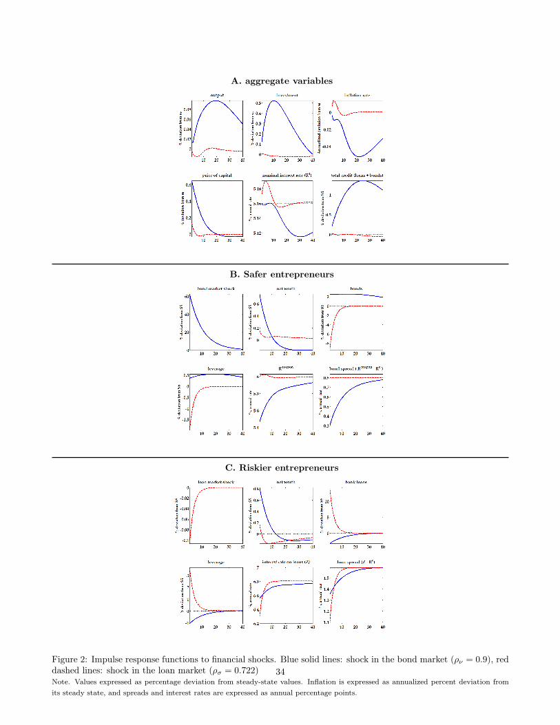
A. aggregate variables
B. Safer entrepreneurs
C. Riskier entrepreneurs
Figure 2: Impulse response functions to financial shocks. Blue solid lines: shock in the bond market (ρν = 0.9), reddashed lines: shock in the loan market (ρσ = 0.722)Note. Values expressed as percentage deviation from steady-state values. Inflation is expressed as annualized percent deviation fromits steady state, and spreads and interest rates are expressed as annual percentage points.
34

A. ATR1 - response to asset prices
B. ATR2 - response to credit growth
C. ATR3a - response to bond spread
Figure 3: Standardized loss implied by alternative augmented Taylor rules for different policy regimes (shock in thebond market, ρν = 0.9).Note. LF 1 = var (π); LF 2 = var (π) + var(y); LF 3 = var (π) + 0.5var(y); LF 4 = var (π) + 0.1var(y); LF 5 = var (π) + 0.5var(y) +
0.1var (∆Re); LF 6 = var (π) + 0.1var(y) + 0.1var (∆Re).
35

A. ATR1 - response to asset prices
B. ATR2 - response to credit growth
C. ATR3b - response to loan spread
Figure 4: Standardized loss implied by alternative augmented Taylor rules for different policy regimes (shock in theloan market, ρσ = 0.722).Note. LF 1 = var (π); LF 2 = var (π) + var(y); LF 3 = var (π) + 0.5var(y); LF 4 = var (π) + 0.1var(y); LF 5 = var (π) + 0.5var(y) +
0.1var (∆Re); LF 6 = var (π) + 0.1var(y) + 0.1var (∆Re).
36

Figure5:
Impu
lserespon
sefunction
sto
abo
ndmarketshock(ρν
=0.
9)un
derdiffe
rent
Taylorrules
Note.
Black
lines:BTR.Bluelin
es:ATR1(top
panel:φq
=0.1
35;bo
ttom
panel:φq
=0.0
6).
Red
lines:ATR2(top
panel:φ∆credit
=0.3
3;bo
ttom
panel:
φ∆credit
=0.1
8).
Green
lines:ATR3a
(top
panel:φbs
=0.3
5;bo
ttom
panel:φbs
=0.0
6).
Infla
tion
isexpressedas
annu
alized
percentdeviationfrom
itssteady
state,
output
aspe
rcentage
deviationfrom
itssteady
state,
andno
minal
interest
rate
asan
nual
percentage
points.
37

Figure6:
Impu
lserespon
sefunction
sto
aloan
marketshock(ρσ
=0.
722)un
derdiffe
rent
Taylorrules
Note.
Black
lines:BTR.Bluelin
es:ATR1(top
panel:φq
=0.2
3;bo
ttom
panel:φq
=0.4
95).
Red
lines:ATR2(top
panel:φ∆credit
=0.2
8;bo
ttom
panel:
φ∆credit
=0.0
7).
Green
lines:ATR3a
(top
panel:φls
=0.0
15;bo
ttom
panel:φls
=0.2
35).
Infla
tion
isexpressedas
annu
alized
percentdeviationfrom
itssteady
state,
output
aspe
rcentage
deviationfrom
itssteady
state,
andno
minal
interest
rate
asan
nual
percentage
points.
38
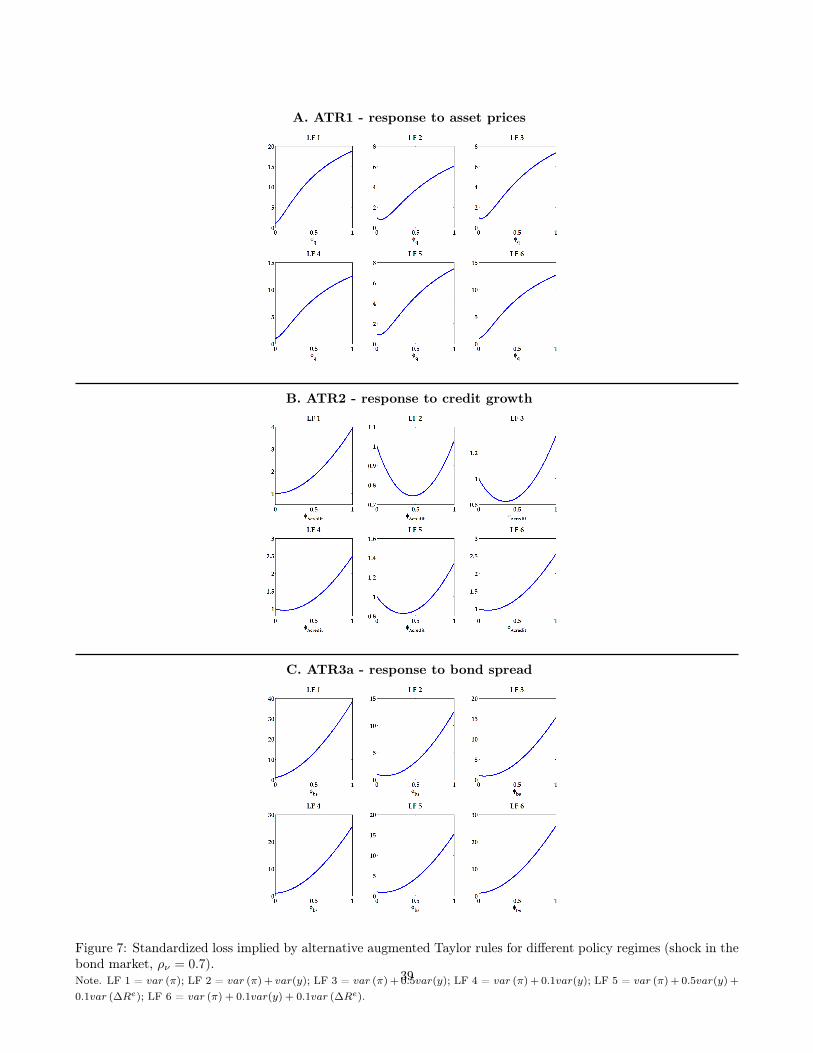
A. ATR1 - response to asset prices
B. ATR2 - response to credit growth
C. ATR3a - response to bond spread
Figure 7: Standardized loss implied by alternative augmented Taylor rules for different policy regimes (shock in thebond market, ρν = 0.7).Note. LF 1 = var (π); LF 2 = var (π) + var(y); LF 3 = var (π) + 0.5var(y); LF 4 = var (π) + 0.1var(y); LF 5 = var (π) + 0.5var(y) +
0.1var (∆Re); LF 6 = var (π) + 0.1var(y) + 0.1var (∆Re).
39

A. ATR1 - response to asset prices
B. ATR2 - response to credit growth
C. ATR3b - response to loan spread
Figure 8: Standardized loss implied by alternative augmented Taylor rules for different policy regimes (shock in theloan market, ρσ = 0.9).Note. LF 1 = var (π); LF 2 = var (π) + var(y); LF 3 = var (π) + 0.5var(y); LF 4 = var (π) + 0.1var(y); LF 5 = var (π) + 0.5var(y) +
0.1var (∆Re); LF 6 = var (π) + 0.1var(y) + 0.1var (∆Re).40
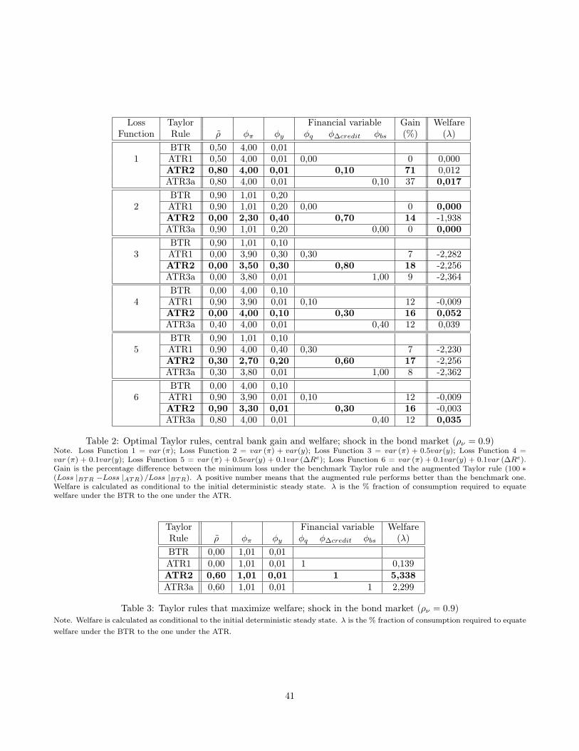
Loss Taylor Financial variable Gain WelfareFunction Rule ρ φπ φy φq φ∆credit φbs (%) (λ)
BTR 0,50 4,00 0,011 ATR1 0,50 4,00 0,01 0,00 0 0,000
ATR2 0,80 4,00 0,01 0,10 71 0,012ATR3a 0,80 4,00 0,01 0,10 37 0,017BTR 0,90 1,01 0,20
2 ATR1 0,90 1,01 0,20 0,00 0 0,000ATR2 0,00 2,30 0,40 0,70 14 -1,938ATR3a 0,90 1,01 0,20 0,00 0 0,000BTR 0,90 1,01 0,10
3 ATR1 0,00 3,90 0,30 0,30 7 -2,282ATR2 0,00 3,50 0,30 0,80 18 -2,256ATR3a 0,00 3,80 0,01 1,00 9 -2,364BTR 0,00 4,00 0,10
4 ATR1 0,90 3,90 0,01 0,10 12 -0,009ATR2 0,00 4,00 0,10 0,30 16 0,052ATR3a 0,40 4,00 0,01 0,40 12 0,039BTR 0,90 1,01 0,10
5 ATR1 0,90 4,00 0,40 0,30 7 -2,230ATR2 0,30 2,70 0,20 0,60 17 -2,256ATR3a 0,30 3,80 0,01 1,00 8 -2,362BTR 0,00 4,00 0,10
6 ATR1 0,90 3,90 0,01 0,10 12 -0,009ATR2 0,90 3,30 0,01 0,30 16 -0,003ATR3a 0,80 4,00 0,01 0,40 12 0,035
Table 2: Optimal Taylor rules, central bank gain and welfare; shock in the bond market (ρν = 0.9)Note. Loss Function 1 = var (π); Loss Function 2 = var (π) + var(y); Loss Function 3 = var (π) + 0.5var(y); Loss Function 4 =var (π) + 0.1var(y); Loss Function 5 = var (π) + 0.5var(y) + 0.1var (∆Re); Loss Function 6 = var (π) + 0.1var(y) + 0.1var (∆Re).Gain is the percentage difference between the minimum loss under the benchmark Taylor rule and the augmented Taylor rule (100 ∗(Loss |BTR −Loss |ATR) /Loss |BTR). A positive number means that the augmented rule performs better than the benchmark one.Welfare is calculated as conditional to the initial deterministic steady state. λ is the % fraction of consumption required to equatewelfare under the BTR to the one under the ATR.
Taylor Financial variable WelfareRule ρ φπ φy φq φ∆credit φbs (λ)BTR 0,00 1,01 0,01ATR1 0,00 1,01 0,01 1 0,139ATR2 0,60 1,01 0,01 1 5,338ATR3a 0,60 1,01 0,01 1 2,299
Table 3: Taylor rules that maximize welfare; shock in the bond market (ρν = 0.9)Note. Welfare is calculated as conditional to the initial deterministic steady state. λ is the % fraction of consumption required to equatewelfare under the BTR to the one under the ATR.
41
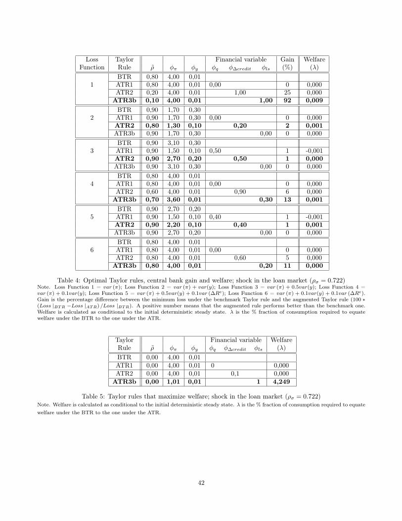
Loss Taylor Financial variable Gain WelfareFunction Rule ρ φπ φy φq φ∆credit φls (%) (λ)
BTR 0,80 4,00 0,011 ATR1 0,80 4,00 0,01 0,00 0 0,000
ATR2 0,20 4,00 0,01 1,00 25 0,000ATR3b 0,10 4,00 0,01 1,00 92 0,009BTR 0,90 1,70 0,30
2 ATR1 0,90 1,70 0,30 0,00 0 0,000ATR2 0,80 1,30 0,10 0,20 2 0,001ATR3b 0,90 1,70 0,30 0,00 0 0,000BTR 0,90 3,10 0,30
3 ATR1 0,90 1,50 0,10 0,50 1 -0,001ATR2 0,90 2,70 0,20 0,50 1 0,000ATR3b 0,90 3,10 0,30 0,00 0 0,000BTR 0,80 4,00 0,01
4 ATR1 0,80 4,00 0,01 0,00 0 0,000ATR2 0,60 4,00 0,01 0,90 6 0,000ATR3b 0,70 3,60 0,01 0,30 13 0,001BTR 0,90 2,70 0,20
5 ATR1 0,90 1,50 0,10 0,40 1 -0,001ATR2 0,90 2,20 0,10 0,40 1 0,001ATR3b 0,90 2,70 0,20 0,00 0 0,000BTR 0,80 4,00 0,01
6 ATR1 0,80 4,00 0,01 0,00 0 0,000ATR2 0,80 4,00 0,01 0,60 5 0,000ATR3b 0,80 4,00 0,01 0,20 11 0,000
Table 4: Optimal Taylor rules, central bank gain and welfare; shock in the loan market (ρσ = 0.722)Note. Loss Function 1 = var (π); Loss Function 2 = var (π) + var(y); Loss Function 3 = var (π) + 0.5var(y); Loss Function 4 =var (π) + 0.1var(y); Loss Function 5 = var (π) + 0.5var(y) + 0.1var (∆Re); Loss Function 6 = var (π) + 0.1var(y) + 0.1var (∆Re).Gain is the percentage difference between the minimum loss under the benchmark Taylor rule and the augmented Taylor rule (100 ∗(Loss |BTR −Loss |ATR) /Loss |BTR). A positive number means that the augmented rule performs better than the benchmark one.Welfare is calculated as conditional to the initial deterministic steady state. λ is the % fraction of consumption required to equatewelfare under the BTR to the one under the ATR.
Taylor Financial variable WelfareRule ρ φπ φy φq φ∆credit φls (λ)BTR 0,00 4,00 0,01ATR1 0,00 4,00 0,01 0 0,000ATR2 0,00 4,00 0,01 0,1 0,000ATR3b 0,00 1,01 0,01 1 4,249
Table 5: Taylor rules that maximize welfare; shock in the loan market (ρσ = 0.722)Note. Welfare is calculated as conditional to the initial deterministic steady state. λ is the % fraction of consumption required to equatewelfare under the BTR to the one under the ATR.
42
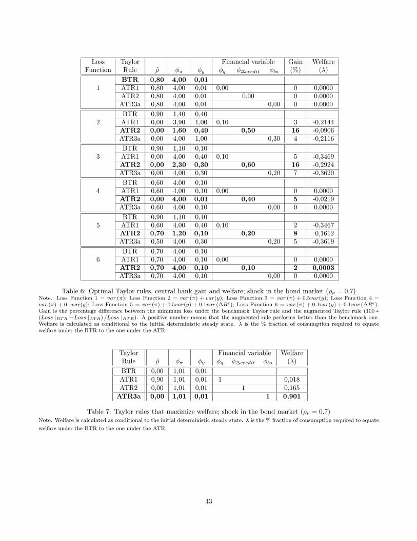
Loss Taylor Financial variable Gain WelfareFunction Rule ρ φπ φy φq φ∆credit φbs (%) (λ)
BTR 0,80 4,00 0,011 ATR1 0,80 4,00 0,01 0,00 0 0,0000
ATR2 0,80 4,00 0,01 0,00 0 0,0000ATR3a 0,80 4,00 0,01 0,00 0 0,0000BTR 0,90 1,40 0,40
2 ATR1 0,00 3,90 1,00 0,10 3 -0,2144ATR2 0,00 1,60 0,40 0,50 16 -0,0906ATR3a 0,00 4,00 1,00 0,30 4 -0,2116BTR 0,90 1,10 0,10
3 ATR1 0,00 4,00 0,40 0,10 5 -0,3469ATR2 0,00 2,30 0,30 0,60 16 -0,2924ATR3a 0,00 4,00 0,30 0,20 7 -0,3620BTR 0,60 4,00 0,10
4 ATR1 0,60 4,00 0,10 0,00 0 0,0000ATR2 0,00 4,00 0,01 0,40 5 -0,0219ATR3a 0,60 4,00 0,10 0,00 0 0,0000BTR 0,90 1,10 0,10
5 ATR1 0,60 4,00 0,40 0,10 2 -0,3467ATR2 0,70 1,20 0,10 0,20 8 -0,1612ATR3a 0,50 4,00 0,30 0,20 5 -0,3619BTR 0,70 4,00 0,10
6 ATR1 0,70 4,00 0,10 0,00 0 0,0000ATR2 0,70 4,00 0,10 0,10 2 0,0003ATR3a 0,70 4,00 0,10 0,00 0 0,0000
Table 6: Optimal Taylor rules, central bank gain and welfare; shock in the bond market (ρν = 0.7)Note. Loss Function 1 = var (π); Loss Function 2 = var (π) + var(y); Loss Function 3 = var (π) + 0.5var(y); Loss Function 4 =var (π) + 0.1var(y); Loss Function 5 = var (π) + 0.5var(y) + 0.1var (∆Re); Loss Function 6 = var (π) + 0.1var(y) + 0.1var (∆Re).Gain is the percentage difference between the minimum loss under the benchmark Taylor rule and the augmented Taylor rule (100 ∗(Loss |BTR −Loss |ATR) /Loss |BTR). A positive number means that the augmented rule performs better than the benchmark one.Welfare is calculated as conditional to the initial deterministic steady state. λ is the % fraction of consumption required to equatewelfare under the BTR to the one under the ATR.
Taylor Financial variable WelfareRule ρ φπ φy φq φ∆credit φbs (λ)BTR 0,00 1,01 0,01ATR1 0,90 1,01 0,01 1 0,018ATR2 0,00 1,01 0,01 1 0,165ATR3a 0,00 1,01 0,01 1 0,901
Table 7: Taylor rules that maximize welfare; shock in the bond market (ρν = 0.7)Note. Welfare is calculated as conditional to the initial deterministic steady state. λ is the % fraction of consumption required to equatewelfare under the BTR to the one under the ATR.
43

Loss Taylor Financial variable Gain WelfareFunction Rule ρ φπ φy φq φ∆credit φls (%) (λ)
BTR 0,70 4,00 0,011 ATR1 0,70 4,00 0,01 0,80 72 -0,001
ATR2 0,40 4,00 0,01 0,50 63 -0,001ATR3b 0,40 4,00 0,01 0,30 87 0,002BTR 0,90 1,40 0,20
2 ATR1 0,90 1,40 0,20 0,00 0 0,000ATR2 0,90 1,50 0,20 0,10 3 0,002ATR3b 0,90 1,40 0,20 0,00 0 0,000BTR 0,90 2,80 0,20
3 ATR1 0,90 1,40 0,10 0,10 7 -0,005ATR2 0,90 1,80 0,10 0,20 8 0,000ATR3b 0,90 1,80 0,20 0,10 4 -0,002BTR 0,80 4,00 0,01
4 ATR1 0,90 4,00 0,10 0,40 13 -0,001ATR2 0,80 4,00 0,01 0,30 12 0,000ATR3b 0,80 4,00 0,10 0,20 11 0,000BTR 0,90 2,80 0,20
5 ATR1 0,90 1,40 0,10 0,10 7 -0,005ATR2 0,90 1,80 0,10 0,20 8 0,000ATR3b 0,90 1,80 0,20 0,10 4 -0,002BTR 0,80 4,00 0,01
6 ATR1 0,90 4,00 0,01 0,30 13 0,000ATR2 0,90 4,00 0,01 0,30 12 0,000ATR3b 0,90 4,00 0,01 0,10 10 0,001
Table 8: Optimal Taylor rules, central bank gain and welfare; shock in the loan market (ρσ = 0.9)Note. Loss Function 1 = var (π); Loss Function 2 = var (π) + var(y); Loss Function 3 = var (π) + 0.5var(y); Loss Function 4 =var (π) + 0.1var(y); Loss Function 5 = var (π) + 0.5var(y) + 0.1var (∆Re); Loss Function 6 = var (π) + 0.1var(y) + 0.1var (∆Re).Gain is the percentage difference between the minimum loss under the benchmark Taylor rule and the augmented Taylor rule (100 ∗(Loss |BTR −Loss |ATR) /Loss |BTR). A positive number means that the augmented rule performs better than the benchmark one.Welfare is calculated as conditional to the initial deterministic steady state. λ is the % fraction of consumption required to equatewelfare under the BTR to the one under the ATR.
Taylor Financial variable WelfareRule ρ φπ φy φq φ∆credit φls (λ)BTR 0,90 1,60 0,01ATR1 0,90 1,60 0,01 0 0,000ATR2 0,00 1,01 0,01 0,70 0,684ATR3b 0,00 1,01 0,01 1 9,215
Table 9: Taylor rules that maximize welfare; shock in the loan market (ρσ = 0.9)Note. Welfare is calculated as conditional to the initial deterministic steady state. λ is the % fraction of consumption required to equatewelfare under the BTR to the one under the ATR.
44

Loss Taylor Financial variable Gain WelfareFunction Rule ρ φπ φy φq φ∆credit φbs φls (%) (λ)
BTR 0,70 4,00 0,01ATR1 0,70 4,00 0,01 0,00 0 0,000
1 ATR2 0,80 4,00 0,01 0,10 24 0,018ATR3a 0,80 4,00 0,01 0,10 12 0,023ATR3b 0,80 4,00 0,01 0,40 54 0,032BTR 0,90 1,10 0,20ATR1 0,90 1,10 0,20 0,00 0 0,000
2 ATR2 0,00 1,80 0,30 0,50 13 -0,977ATR3a 0,90 1,10 0,20 0,00 0 0,000ATR3b 0,90 1,01 0,10 0,10 0 0,940BTR 0,90 1,01 0,10ATR1 0,90 4,00 0,40 0,30 7 -2,212
3 ATR2 0,00 2,70 0,20 0,60 17 -2,241ATR3a 0,00 3,80 0,01 1,00 8 -2,344ATR3b 0,90 1,20 0,10 0,20 2 -1,728BTR 0,60 4,00 0,10ATR1 0,90 4,00 0,01 0,10 13 -0,004
4 ATR2 0,70 4,00 0,01 0,30 17 0,000ATR3a 0,80 4,00 0,01 0,40 13 0,041ATR3b 0,00 4,00 0,01 0,80 14 0,015BTR 0,90 1,01 0,10ATR1 0,90 4,00 0,40 0,30 7 -2,212
5 ATR2 0,60 2,40 0,20 0,50 17 -2,200ATR3a 0,50 3,80 0,01 1,00 7 -2,340ATR3b 0,90 1,20 0,10 0,20 2 -1,728BTR 0,70 4,00 0,10ATR1 0,90 4,00 0,01 0,10 13 -0,001
6 ATR2 0,80 4,00 0,01 0,30 17 0,000ATR3a 0,80 4,00 0,01 0,40 14 0,044ATR3b 0,80 4,00 0,10 0,60 11 0,048
Table 10: Optimal unconditional Taylor rules, central bank gain and welfareNote. Loss Function 1 = var (π); Loss Function 2 = var (π) + var(y); Loss Function 3 = var (π) + 0.5var(y); Loss Function 4 =var (π) + 0.1var(y); Loss Function 5 = var (π) + 0.5var(y) + 0.1var (∆Re); Loss Function 6 = var (π) + 0.1var(y) + 0.1var (∆Re).Gain is the percentage difference between the minimum loss under the benchmark Taylor rule and the augmented Taylor rule (100 ∗(Loss |BTR −Loss |ATR) /Loss |BTR). A positive number means that the augmented rule performs better than the benchmark one.Welfare is calculated as conditional to the initial deterministic steady state. λ is the % fraction of consumption required to equatewelfare under the BTR to the one under the ATR.
Taylor Financial variable WelfareRule ρ φπ φy φq φ∆credit φbs φls (λ)BTR 0,00 1,01 0,01ATR1 0,00 1,01 0,01 1 0,144ATR2 0,60 1,01 0,01 1 5,341ATR3a 0,60 1,01 0,01 1 2,307ATR3b 0,00 1,01 0,01 1 14,291
Table 11: Unconditional Taylor rules that maximize welfareNote. Welfare is calculated as conditional to the initial deterministic steady state. λ is the % fraction of consumption required to equatewelfare under the BTR to the one under the ATR.
45
Top Related