


Languages
Pages
Legal


Journal of Economics, Business and Management, Vol. 3, No. 7, July 2015
DOI: 10.7763/JOEBM.2015.V3.275 731
Abstract—This paper examines monetary independence
during the period when Malaysia had a fixed exchange rate and
an open capital account regime. The objective is to assess the
relevance of the Impossible Trinity for policy. The evidence of
cointegration between the Malaysian and US interest rates
during this period, suggests that there is no monetary
independence in the long run. However, our results show there
is: Malaysia retains some monetary autonomy in the short run.
The loss of long-run monetary autonomy under peg/open
capital was in line with the trinity, and may be one reason the
peg was eventually abandoned for managed floating in July
2005.
Index Terms—Impossible trinity, Malaysia.
I. INTRODUCTION
The impossible trinity postulates that it is impossible to
have a fixed exchange rate regime, an open capital account
and an independent monetary policy simultaneously. A
country can choose only two of these goals, but not all of
them simultaneously. If a country chooses a fixed exchange
rate and an open capital account, it means it has to forgo an
independent monetary policy. In other words, the cost of
maintaining a fixed exchange rate and an open capital
account is a loss of control over the domestic monetary policy,
as domestic interest rates will be correlated with the pegged
country rates. This hypothesis has been widely taught and
recognized since it is quite intuitive and helpful to understand
the constraints policy makers must face in an open economy
setting.
Empirical examination of the nature of these tradeoffs is
not abundant. Ohanian and Stockman [1] showed that there
can be in fact some room for an independent monetary policy
in the short run under a fixed exchange rate regime. Svensson
[2] found similar evidence of short-term monetary
independence within the EMS. Lim and Goh [3] tested for
monetary independence in Malaysia by estimating the capital
account offset and sterilization coefficients. Their results are
consistent with [1] in that the Malaysian central bank
possesses some short-run control over monetary policy even
during the fixed exchange rate regime. This is in sharp
contrast to the impossible trinity’s argument, which states
that a country will lose all its monetary independence under
fixed exchange rates and free capital mobility.
The objective of this paper is to test the trilemma
predictions using a small, emerging market, that is, Malaysia
Manuscript received December 18, 2013; revised February 20, 2014.
This work was supported by the Short Term Research Grant,
304/CDASAR/6311107, Universiti Sains Malaysia.
Soo Khoon Goh is with the Universiti Sains Malaysia (e-mail:
in the 2000s. During the Asian Currency Crisis, Malaysia
pegged its ringgit to the US dollar and imposed capital
controls in Sept, 1998. By May, 2001, Malaysia lifted its
capital controls but kept the peg before it removed the peg in
July 2005. During this period, the trilemma would predict
that Malaysia would have no choice but to give up its
monetary autonomy, i.e. allow its interest rates to move
closely with the US rates. We aim to examine the correlation
between the Malaysian and US interest rates during this
period, by using cointegration techniques. The hypothesis is
that if the trinity holds, there should be no monetary policy
autonomy in Malaysia, when Malaysia has a fixed exchange
rate and an open capital account. Interest rates in Malaysia
should move closely with the interest rates in US, in order to
maintain the pegged exchange rate. Hence, we should find
evidence of cointegration between Malaysian and US interest
rates from May 2001 till June 2005.
Thus far, there has only been one econometric study of the
effects of the trilemma on Malaysia’s monetary policy in this
period. Lim and Goh [3] tested for monetary independence
but not interest rate independence by estimating capital
account offset and sterilization coefficients. Their results
suggest that even though BNM had some monetary control in
the short run, it, however, lost its long-run monetary control
during the peg/open capital period, and only re-captured
control when it switched to managed floating1. Our study will
differ from [3] in that we will use interest rate
interdependence as the indicator for monetary independence.
It will be interesting to see if a different indicator would
suggest the same conclusions as the 2011 study; and why, if it
should not.
The remainder of the paper is as follows. Section 2 deals
with the theoretical framework and empirical methodology
used in this paper. Section 3 reports and discusses the test
results. The main conclusions and policy implications can be
found in the last section.
II. THE MODEL AND THE METHODOLOGY
We illustrate the underlying monetary independence
hypothesis using the uncovered interest parity condition
(UIP). The UIP is expressed as:
*
1( )t t t ti i E s s (1)
where i is the nominal interest rate, i* is the base country
interest rate2, s is the exchange rate, E is the expectation
1For the period prior to the Asian Currency Crisis (managed floating),
Takagawa[4] and Umezaki [5] also found that Malaysia enjoyed some
degree of monetary independence. 2 The base country is the economy in which a country is pegged.
Can a Country be Exempted from Impossible Trinity:
Evidence from Malaysia
Soo Khoon Goh
Journal of Economics, Business and Management, Vol. 3, No. 7, July 2015
732
operator, ρ is the risk premium and t is the time operator.
Under a fixed exchange rate regime, st is constant. In a
fully credible peg, we would expect that 1( tE s
) remain the
same, hence, the third term can be dropped as zero. Similarly,
in the absence of any risk premium, ρ is expected to be zero.
Hence, for a credible peg under open capital account, the
domestic interest rates are expected to move one-for-one with
the base country interest rates, that is:
*
t ti i (2)
In other words, there is a loss of monetary autonomy under
a fixed exchange rate and an open capital regime.
Under a floating exchange rate regime, the domestic and
base country interest rates are independent and only the spot
exchange rate (e) adjusts to satisfy the UIP condition. The
expected change in exchange rate is equal to interest rate
differential and the risk premium, ρ.
*
1( )t t t tE s s i i (3)
This suggests that economies having floating exchange
rate regimes experience less correlations between domestic
and base country interest rate changes, and hence, have more
monetary autonomy than do economies with fixed exchange
rate regimes. If domestic monetary policy is independent of
monetary policy in the base country, we would expect no
cointegrating relationship between the interest rates. If the
domestic interest rate follows tightly the movements in the
base country’s interest rate, then the domestic monetary
policy is likely to be dependent on the base country’s
monetary policy; and we would expect a strong cointegrating
relationship between the two interest rates. Nevertheless, our
cointegration test implicitly imposes a conditional
relationship between the US and Malaysian interest rate, i.e.
for a small country like Malaysia, the interest rate does not
Granger-cause the US interest rate. In other words, we are
establishing cointegration with weak exogeneity of the
Malaysian interest rate.
Prior to the cointegration test, we would conduct unit root
tests to determine whether the variables are non-stationary
(i.e. have unit roots). If all the variables studied are I (1)
non-stationary, we would proceed to the Johansen maximum
likelihood method [6]-[8] to test whether these variables are
cointegrated. The Johansen approach allows the testing of the
long-run relationship between the variables in a multivariate
framework, and requires that all the variables be of equal
degree of integration to yield estimators which are
super-consistent.
III. DATA DESCRIPTION AND EMPIRICAL RESULTS
We used the Malaysian interbank overnight and US
Federal Fund rates as an indication of policy rate to examine
whether interest rates in Malaysia are forced to follow a
relationship with US interest rates, or whether some deviation
is possible.
The US interest rate data were extracted from the Board of
Governors of the Federal Reserve System, Economic
Research and data website while the Malaysian interbank
rates were extracted from Bank Negara Malaysia, Monthly
Statistics Bulletin.
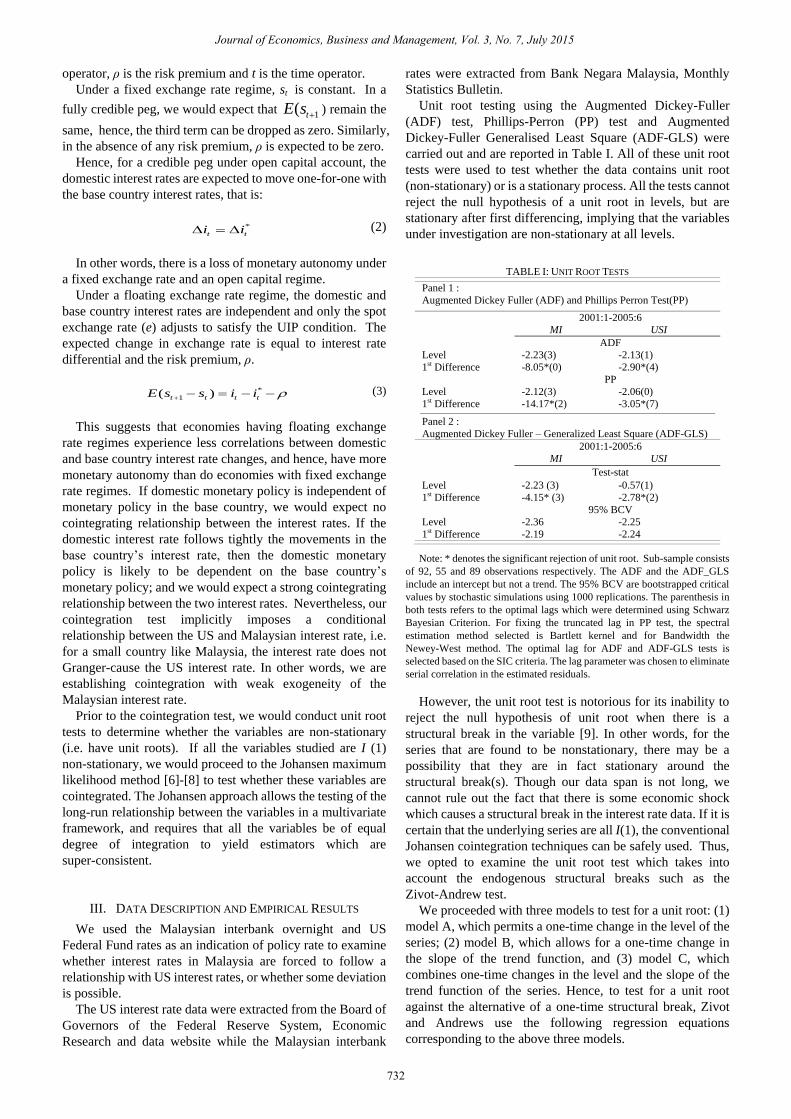
Unit root testing using the Augmented Dickey-Fuller
(ADF) test, Phillips-Perron (PP) test and Augmented
Dickey-Fuller Generalised Least Square (ADF-GLS) were
carried out and are reported in Table I. All of these unit root
tests were used to test whether the data contains unit root
(non-stationary) or is a stationary process. All the tests cannot
reject the null hypothesis of a unit root in levels, but are
stationary after first differencing, implying that the variables
under investigation are non-stationary at all levels.
TABLE I: UNIT ROOT TESTS
Panel 1 :
Augmented Dickey Fuller (ADF) and Phillips Perron Test(PP)
2001:1-2005:6
MI USI
ADF
Level -2.23(3) -2.13(1)
1st Difference -8.05*(0) -2.90*(4)
PP
Level -2.12(3) -2.06(0)
1st Difference -14.17*(2) -3.05*(7)
Panel 2 :
Augmented Dickey Fuller – Generalized Least Square (ADF-GLS)
2001:1-2005:6
MI USI
Test-stat
Level -2.23 (3) -0.57(1)
1st Difference -4.15* (3) -2.78*(2)
95% BCV
Level -2.36 -2.25
1st Difference -2.19 -2.24
Note: * denotes the significant rejection of unit root. Sub-sample consists
of 92, 55 and 89 observations respectively. The ADF and the ADF_GLS
include an intercept but not a trend. The 95% BCV are bootstrapped critical
values by stochastic simulations using 1000 replications. The parenthesis in
both tests refers to the optimal lags which were determined using Schwarz
Bayesian Criterion. For fixing the truncated lag in PP test, the spectral
estimation method selected is Bartlett kernel and for Bandwidth the
Newey-West method. The optimal lag for ADF and ADF-GLS tests is
selected based on the SIC criteria. The lag parameter was chosen to eliminate
serial correlation in the estimated residuals.
However, the unit root test is notorious for its inability to
reject the null hypothesis of unit root when there is a
structural break in the variable [9]. In other words, for the
series that are found to be nonstationary, there may be a
possibility that they are in fact stationary around the
structural break(s). Though our data span is not long, we
cannot rule out the fact that there is some economic shock
which causes a structural break in the interest rate data. If it is
certain that the underlying series are all I(1), the conventional
Johansen cointegration techniques can be safely used. Thus,
we opted to examine the unit root test which takes into
account the endogenous structural breaks such as the
Zivot-Andrew test.
We proceeded with three models to test for a unit root: (1)
model A, which permits a one-time change in the level of the
series; (2) model B, which allows for a one-time change in
the slope of the trend function, and (3) model C, which
combines one-time changes in the level and the slope of the
trend function of the series. Hence, to test for a unit root
against the alternative of a one-time structural break, Zivot
and Andrews use the following regression equations
corresponding to the above three models.
Journal of Economics, Business and Management, Vol. 3, No. 7, July 2015
733
1 1 1( ) (ModelA)t t tY Y DU t e
1 1 2( ) (ModelB)t t tY Y DT t e
1 1 2 3( ) ( ) (ModelC)t t tY Y DU DT t e
where DU is an indicator dummy variable for a mean shift
occurring at each possible break-date (TB) while DT is the
corresponding trend shift variable. The null hypothesis in all
the three models is α=0, which implies that the series {Yt}
contains a unit root with a drift that excludes any structural
break, while the alternative hypothesis α<0 implies that the
series is a trend-stationary process with a one-time break
occurring at an unknown point in time. The Zivot and
Andrews method regards every point as a potential
break-date (TB) and runs a regression for every possible
break-date sequentially. From amongst all possible
break-points (TB), the procedure selects as its choice of
break-date (TB) the date which minimizes the t-statistic.
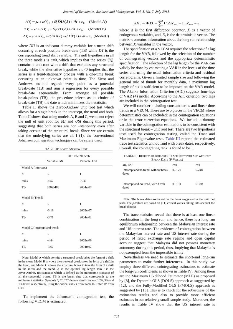
Table II shows the Zivot-Andrew unit root test which
allows for a single break in the intercept, the trend and both.
Table II shows that using models A, B and C, we do not reject
the null of unit root for MI and USI during this period,
suggesting that both series are non –stationary even after
taking account of the structural break. Since we are certain
that the underlying series are all I (1), the conventional
Johansen cointegration techniques can be safely used.
TABLE II: ZIVOT-ANDREW TEST
2001m5: 2005m6
Variable: Mi Variable: USI
Model A (intercept)
K 3 1
min t -4.52 -3.37
TB 2002M06 2004m07
Model B (Trend)
K 3 1
min t -3.16 2002m07
TB -3.71 2004m02
Model C (intercept and trend)
K 3 1
min t -4.44 2002m06
TB -3.67 2004m02
Note: Model A which permits a structural break takes the form of a shift
in the mean, Model B is where the structural break takes the form of a shift in
the trend, and Model C allows the structural break to take the form of a shift
in the mean and the trend. K is the optimal lag length min t is the
Zivot-Andrew test statistics which is defined as the minimum t-statistics of
all the sequential t-tests. TB is the break date that corresponds to the
minimum t statistics. Symbols *, **, *** denote significance at 10%, 5% and
1% levels respectively, using the critical values from Table II- Table IV from
[10].
To implement the Johansen’s cointegration test, the
following VECM is estimated.
1
1
1
k
t t i t i t t
i
X D X X
where Δ is the first difference operator, Xt is a vector of
endogenous variables, and, Dt is the deterministic vector. The
matrix π contains information about the long run relationship
between Xt variables in the vector.
The specification of a VECM requires the selection of a lag
length for the VAR, followed by the selection of the number
of cointegrating vectors and the appropriate deterministic
specification. The selection of the lag length for the VAR can
validly be done by estimating a VAR in the levels of the time
series and using the usual information criteria and residual
correlograms. Given a limited sample size and following the
general rule of thumb for monthly data, a maximum lag
length of six is sufficient to be imposed on the VAR model.
The Akaike Information Criterion (AIC) suggests four-lags
or VAR (4) model. According to the AIC criterion, two lags
are included in the cointegration test.
We will consider including constant terms and linear time
trends in a VECM. There are two places in the VECM where
deterministics can be included: in the cointegration equations
or in the error correction equations. We include a dummy
variable in the cointegration estimations to be consistent with
the structural break – unit root test. There are two hypothesis
tests used for cointegration testing, called the Trace and
Maximum Eigenvalue tests. Table III reports the estimated
trace test statistics without and with break dates, respectively.
Overall, the cointegrating rank is found to be 1.
TABLE III: RESULTS OF JOHANSEN TRACE TEST WITH AND WITHOUT
BREAK DATE (P-VALUE)
MI, USI r=0 r=1
Intercept and no trend, without break
dates
0.0120 0.248
Intercept and no trend, with break
dates
0.0131 0.330
Note: The break dates are based on the dates suggested in the unit root
tests. The p-values are based on [11] critical values taking into account the
break date(s).
The trace statistics reveal that there is at least one linear
combination in the long run, and hence, there is a long run
equilibrium relationship between the Malaysian interest rate
and US interest rate. The evidence of cointegration between
the Malaysian interest rate and US interest rate during the
period of fixed exchange rate regime and open capital
account suggest that Malaysia did not possess monetary
autonomy during this period, thus, implying that Malaysia is
not exempted from the impossible trinity.
Nevertheless we need to estimate the short-and long-run
parameters to make further inferences. In this study, we
employ three different cointegrating estimators to estimate
the long-run coefficients as shown in Table IV. Among them
are the Maximum Likelihood Estimator (MLE) as proposed
by [8], the Dynamic OLS (DOLS) approach as suggested by
[12], and the Fully-Modified OLS (FMOLS) approach as
suggested by [13]. This is to check for the robustness of the
estimation results and also to provide more efficient
estimates in our relatively small sample study. Moreover, the
results in Table IV show that the US interest rate is
Journal of Economics, Business and Management, Vol. 3, No. 7, July 2015
734
statistically significant across the different cointegrating
equation estimators.
TABLE IV: THE LONG-RUN ESTIMATES
MLE FMOLS DOLS
Intercept 1.56***
(0.12)
3.74**
(0.26)
2.00***
(0.34)
USI 0.31***
(0.10)
0.44***
(0.09)
0.20**
(0.09)
Dummy 1.13***
(0.20)
3.74***
(0.26)
0.70***
(0.23)
Note: We estimate r on r* where r is the interest rate in Malaysia and r* is
the interest rate in US. Our model includes an intercept and the dummies for
period 2002:6 onwards. For DOLS, the lags and leads are each set to 1 and 1.
For FMOLS, the optimal lags were set using the AIC criteria. Parentheses
indicate standard error. *, ** and *** denote significant levels at 10%, 5%
and 1% respectively.
The Error-Correction Model (ECM) is estimated to derive
the short-run parameters as shown below:
1 10.015 0.41 0.71
(0.02) (0.09) (0.31)
t t tmi ECT mi
2 3 40.97 0.21 0.24
(0.26) (0.15) (0.15)
t t tmi mi mi
1 2 30.44 0.22 0.20
(0.25) (0.25) (0.24)
t t tusi usi usi
4 1 20.42 0.60 0.33
(0.22) (0.31) (0.28)
t t tusi dum dum
3 40.47 0.40
(0.28) (0.28)
t tdum dum
R2=0.72, F-stat=6.28, Log-likelihood=31.71, where the
parentheses contain the standard errors.
The ECM shows that the Error Correction Term (ECT) is
highly significant and negative suggesting that 41 percent of
the disequilibrium is eliminated within one period (i.e. one
month in this study). There is no 100% adjustment to
eliminate the disequilibrium in a single month; we interpret
that BNM does retain some short run monetary autonomy
during the period concerned. We attribute this short term
monetary autonomy to sterilization activities conducted by
BNM [3]. BNM undertook active sterilization operations to
absorb the capital inflows to avoid excessive liquidity in the
domestic financial market since the installation of the fixed
exchange rate regime.
IV. CONCLUDING REMARKS
We used a cointegration framework to examine whether
Malaysian interest rates are driven by the US’s interest rates
during the fixed exchange and open capital account regime.
We were careful in determining the order of integration of the
underlying variables in the model prior to the cointegration
test. This is important to ensure that Johansen cointegration
test is an appropriate test in this study.
Upon very careful inspection of the Johansen tests, we
found evidence that Malaysia’s interest rate cointegrated with
the interest rate in the US during the period of fixed exchange
rate and open capital account regimes, suggesting that
Malaysia is not exempted from the impossible trinity.
Our empirical results suggest that the trinity was at work
for Malaysia during the periods of this investigation. It is not
possible to have a fixed exchange rate, monetary policy
autonomy, and open capital markets at the same time. Our
study demonstrates that fixed exchange rates involve a loss of
monetary policy autonomy. If a country wants to have its own
monetary policy, then, it has to let the exchange rate float
freely in an open capital account regime. In other words, a
combination of an open capital account, a fixed exchange rate
and an independent monetary policy is not possible. That
explains why Malaysia moved away from a fixed exchange
rate to a managed float on 21 July, 2005.
REFERENCES
[1] L. E. Ohanian and A. C. Stockman, “Short-run independence of
monetary policy under pegged exchange rates and effects of money on
exchange rates and interest rates,” Journal of Money, Credit and
Banking, vol. 29, no. 4, pp. 783-806, 1998.
[2] L. Svensson, “Why exchange rate bands? Monetary independence in
spite of fixed exchange rates,” Journal of Monetary Economics, vol. 33,
pp. 157-199, 1994.
[3] E. G. Lim, and S. K. Goh, “Is Malaysia exempted from impossible
trinity: Evidence from 1991 to 2009,” CenPRIS Working Paper,
139/11, 2011.
[4] I. Takagawa, “An empirical analysis of the impossible trinity,” in
Exchange Rates, Capital Flows and Policy, ed, R. Driver, Sinclair, and
C. Thoenissen, UK: Routledge, 2005, pp. 15-30.
[5] S. Umezaki, “Monetary policy in a small open economy: The case of
Malaysia,” The Developing Economies, vol. XLV-4, pp. 437-464,
2007.
[6] S. Johansen, “Statisical analysis of cointegrating vector,” Journal of
Economic Dynamics and Control, vol. 12, pp. 231-254, 1988.
[7] S. Johansen, “Estimation and hypothesis testing of cointegration
vectors in Gaussian vector autoregressive models,” Econometrica, vol.
59, pp. 1551-1580, 1991.
[8] S. Johansen and K. Juselius, “Maximum likelihood estimation and
inference on cointegration with applications to the demand for money,”
Oxford Bulletin of Economics and Statistics, vol. 52, pp. 169-210,
1990.
[9] P. Perron, “The great crash, the oil price shock and the unit root
hypothesis,” Econometrica, vol. 57, pp. 1361-1401, 1989.
[10] E. Zivot and D. Andrews, “Further evidence of the great crash, the
oil-price shock and the unit-root hypothesis,” Journal of Business and
Economic Statistics, vol. 10, pp. 251-270, 1992.
[11] S. Johansen, R. Mosconi, and B. Nielsen, “Cointegration analysis in
the presence of structural breaks in the deterministic trend,”
Econometrics Journal, vol. 3, pp. 216-49, 2000.
[12] J. H. Stock and M. W. Watson, “A simple estimator of cointegrating
vectors in higher order integrated systems,” Econometrica, vol. 61, no.
4, pp. 783-820, 1993.
[13] P. C. B. Phillips and B. E. Hansen, “Statistical inference in
instrumental variable regression with I(1) processes,” Review of
Economic Studies, vol. 57, no. 1, pp. 99-125, 1990.
Soo Khoon Goh is a senior lecturer at the Centre for
Policy Research and International Studies in
Universiti Sains Malaysia. Science University of
Malaysia, Penang, Malaysia. She has a B. Economics
from University Malaya, Malaysia, M.Sc. in
Economics from University of Colorado Boulder,
USA, and a Ph.D. in Economics from University of
Melbourne, Australia. Her main research interests lie
in macroeconomics and international economics. She has published in
reputable international journals such as Applied Economics, Asian
Economic Journal, Journal of Asian Economics, Applied Economics Letters,
Journal of Business Economics and Management, Economic Modeling. She
is also a Fulbright Scholar, 2012-2013.
Top Related