


Languages
Pages
Legal


MIXED MODEL ANALYSES OF CENSORED NORMALDISTRIBUTIONS VIA THE EM ALGORITHM
by
Fraser B. Smith and Ronald W. Helms
Department of Biostatistics, University ofNorth Carolina at Chapel Hill, NC.
Institute of Statistics Mimeo Series No. 1898T
April 1992

MIXED MODEL ANALYSES OF CENSORED NORMAL
DISTRIBUTIONS VIA THE EM ALGORITHM
by
Fraser B. Smith
A Dissertation submitted to the faculty of The University of North Carolina atChapel Hill in partial fulfillment of the requirements of the degree of Doctor ofPhilosophy in the Department of Biostatistics.
Chapel Hill
1992
Advisor
Reader
Reader
Reader
11
ABSTRACT
FRASER B. SMITH. Mixed Model Analyses of Censored Normal Distributions via
the EM Algorithm. (Under the direction of Ronald W. Helms.)
The analysis of censored data from repeated measures and crossover studies is
a frequently occurring problem. The purpose of this work is to develop a method
to estimate parameters in general linear mixed models with fixed censoring,
noninformative random censoring, or informative random censoring. The proposed
method is an extension of maximum likelihood estimation and is applicable to
normal data from longitudinal studies where the effects of serial correlation are
negligible. Current methods dealing with such topics are limited in that no
methods are available to address parameter estimation in general linear mixed
models with nonterminal informative censoring and the methods developed for
fixed and noninformatively censored data are computationally infeasible.
General convergence properties of the EM algorithm described in Cox and
Oakes (1984) for general linear univariate models are discussed. Cox and Oakes
restricted their discussion to fixed censoring where censoring values were considered
to be predetermined constants. These results are extended to the case of general
linear univariate models with noninformative and informative random censoring.
Subsequently this approach is extended so that it can be used for parameter
estimation in general linear mixed models. Unlike previous approaches, this
method has the advantages of not reqUIrIng computations of high-dimensional
integrals, not requiring the inversion of large matrices, and is not restricted to
random intercept models or studies with noninformative or fixed censoring. This
method is applied to data from a placebo-controlled, double-blind crossover, dose-

1ll
ranging study to assess the short-term efficacy of an antianginal drug in patients
with chronic stable angina. Censoring was informative and nonterminal, i.e., was
not due to death or withdrawal from the study.•

IV
ACKNOWLEDGEMENTS
I gratefully acknowledge my dissertation advisor, Dr. Ron Helms, for his
encouragement, guidance, and support, and for the numerous hours he contributed
to this research. I also thank my other committee members, Dr. Gerardo Heiss,
Dr. Jim Hosking, Dr. Larry Kupper, and Dr. Paul Stewart, and acknowledge Dr.
Bahjat Qaqish for his suggestions and comments.
I express my gratitude also to Dr. Bernard Chaitman of the St. Louis
University Medical Center for allowing me to use his data and to Ms. Margery
Cruise and Dr. David Frankel, who introduced me to the Chaitman data while I
was working at Miles Canada in 1986. Finally, I express my deep appreciation to
my family for their encouragement and financial support.

v
TABLE OF CONTENTS
Chapter Page
I. INTRODUCTION AND LITERATURE REVIEW 1
1.1. Introduction 11.2. Literature Review 8
1.2.1. Likelihood Functions: General Linear Univariate Modelswith Noninformative Censoring 11
1.2.2. EM Algorithm 16
1.2.2.1. EM Algorithm for Regular Exponential Families 161.2.2.2. Behavior of the EM Algorithm 201.2.2.3. Derivation of the EM Algorithm;
General Linear Univariate Models with Fixed Censoring ..221.2.2.4. EM Computations;
General Linear Univariate Models with Fixed Censoring ..26
1.2.3. Mixed Models with Noninformative Right Censoringor Fixed Left Censoring 29
1.3. Statement of the Pro1:>lem and Outline. 39
II. GENERAL LINEAR UNIVARIATE MODELSWITH RANDOM CENSORING 43
2.1. General Linear Univariate Modelswith Noninformative Right Censoring .43
2.1.1. Derivation of the EM Algorithm .432.1.2. EM Computations 47
2.2. General Linear Univariate Modelswith Informative Right Censoring 50
2.2.1. Derivation of the EM Algorithm 502.2.2. EM Computations 56

VI
III. MIXED MODELS WITH RANDOM CENSORING 62
3.1. Mixed Models with Noninformative Right Censoring 62
3.1.1. Likelihood Functions 623.1.2. Derivation of the EM Algorithm 673.1.3. EM Computations 74
3.2. Mixed Models with Informative Right Censoring 78
3.2.1. Likelihood Functions 783.2.2. Derivation of the EM Algorithm 883.2.3. EM Computations 93
IV. EXERCISE TOLERANCE TESTS OF PATIENTSWITH CHRONIC STABLE ANGINA 101
4.1. Introduction 1014.2. Description of the Experiment and Data 1034.3. Computational Issues 1054.4. Generation of Data 1094.5. Results 1114.6. Summary 121
V. SUMMARY AND RECOMMENDATIONSFOR FUTURE RESEARCH 122
5.1. Summary 1225.2. Future Research 124
APPENDIX A: Listing of Data From Nisoldipine Crossover Study .......126
APPENDIX B: Listing of Random Sample of 80 Subjects 129
REFERENCES 144

Vll
LIST OF TABLES
Table 1.3.1: Summary of Mixed Model Procedures .41
Table 1.3.2: Dimensions of Matrices that must be Inverted inOrder to Estimate Fixed and Random Effects .42
Table 4.5.1: Parameter Estimates Using Data From Lam et aI.(K=12 Patients) Assuming That No Censoring Occurred 115
Table 4.5.2: Maximum a Posteriori Parameter Estimates Usingthe Randomly Generated Sample (K=80 Patients) 117
Table 4.5.3: Maximum Likelihood Estimates .Using RandomlyGenerated Sample 119

Vlll
LIST OF FIGURES
Figure 4.5.1: Approximate 95% Confidence Intervals forIncremental Effects of Dose and Visit 120
'.
,.
I. INTRODUCTION AND LITERATURE REVIEW
1.1 Introduction
The analysis of incomplete data from repeated measures and crossover studies
is a frequently occurring problem. Data can be incomplete due to:
(a) missing observations where no information is available about the response
of interest, and
(b) truncation or censoring of the response of interest.
Data can be missing or censored for reasons that are either related or unrelated
to the outcome of interest and for reasons that are either planned or accidental.
Unavailable data are said to be missin~ if the experimental protocol specifies that
the data are to be collected but, for reasons beyond the control of the investigator,
the data could not be obtained. Censored data are a special form of incomplete
data in which there is some information about the missing value, namely, that the
data if available, would have been outside a specified bound. For example, if a
device for measuring blood pressure could not measure blood pressure lower than 30
mm Hg or higher than 200 mm Hg, a blood pressure value outside the interval [30,
200] would result in an (unavailable) censored data value.
Censored data problems are common in follow-up studies. For example, in a

2
clinical trial investigating the efficacy of a new treatment for lung cancer the event
of interest could be the survival time of lung cancer patients. Right-censoring
occurs when patients withdraw from the study, die from another cause, or when
they are alive at the end of the study. Note that this is an example of terminal
censorin~ where censoring is due to death or withdrawal from the study and
patients are no longer available for subsequent observation.
Several categories of censoring are important in the context of follow-up
studies: fixed censoring, noninformative random censoring, and informative random
censonng. Fixed censorin~ occurs when the termination of follow-up for each
individual is predetermined in advance. Consequently the censoring values (times
of termination of follow-up) are predetermined constants and censoring occurs if
the event of interest does not occur prior to the scheduled end of follow-up. Note
that censored data values are typically survival· times but in some cases the
"schedule" is based on a variable other than time. For example, in a dose-response
study of the dose required to obtain a 20% reducti<?n in pulmonary function,
censoring typically occurs after a patient reaches a predetermined maximum dose.
Random censoring occurs when the termination of follow-up for each
individual is not predetermined and observation is terminated by a randomly
occurring event prior to the occurrence of the event of interest. The censoring
value is the time to censoring. For example, in a follow-up study of cancer
patients, the censoring time could be the observation time recorded until
observation is terminated because the patient withdraws from the study, as for
example, due to death from a cause other than cancer.
Random censoring is noninformative when the failure values and censormg
<,
3
values are stochastically independent and their distributions depend on two sets of
functionally independent parameters. If the failure values and censoring values are
correlated and/or depend on the same parameters, then the censoring is
informative: the value of the censoring variable carries information about the
distribution of the time-to-failure distribution. In the previous example, censoring
due to withdrawal from the study is informative if patients withdrew because they
were not doing well because of an effect of the treatment or if the probability of
dying from competing causes depends upon whether the subject has cancer.
Data that are missing but not censored can be missing at random, missing
completely at random, or not missing at random. A missing data value is missing
at random if the probability of response is independent of the outcome variable of
interest that would have been observed if the value were not missing (Little and
Rubin 1987, p. 13). A missing data value is missing completely at random if it is
missing at random and if the probability of response is independent of any
predictor variables of the outcome variable of interest.
For the purpose of making likelihood-based inferences, the missing-data
mechanism is ignorable (Little and Rubin 1987, p. 15) if the missing data values
are missing at random. Some examples of ignorably missing data might be: data
that was missing due to laboratory errors, to unrelated illness, or because the
subject moved out of town. Fixed left censored data are clearly not ignorable since
the data values are missing when they fall below a known threshold. Therefore
analysis of a reduced sample excluding the censored data is subject to bias.
To illustrate the difference between missing and censored data, consider an
example in Wei, Lin, and Weissfeld (1989) of a randomized clinical trial to evaluate
the effectiveness of ribavirin, a drug used to treat AIDS patients. Patients were

4
randomized into one of three treatment groups: placebo, low-dose ribavirin and
high-dose ribavirin. Blood samples for each patient were collected after four, eight,
and twelve weeks of treatment. Measurements of p24 antigen levels, important
markers of HIV-1 infection were repeatedly taken for a period of four weeks. The
response of interest was the "viral load" in each blood sample, which was the
number of days until virus positivity (p24>100 picograms/ml) was detected.
Ideally each patient in the study would have had three such event times. However
some observations were missing because patients did not make the scheduled
number of visits or because serum specimens were inadequate for laboratory
analysis. Censoring occurred when the culture required a longer period of time to
register as virus positive than was achievable in the laboratory or when the serum
sample was contaminated during the assay procedure before virus positivity was
detected. The authors assumed that censoring was noninformative and that
missing data were missing at random. Censoring was nonterminal as it was
possible to obtain further blood samples after censoring occurred.
A classic approach used to analyze incomplete longitudinal data is to delete
the entire observation vector (row of Y) for any subject with missing or censored
data and to use multivariate techniques. This process is known as. "casewise"
deletion (Timm 1970). When the proportion of subjects with incomplete data is
high a great deal of information is lost. When the data are not missing at random
this can also be a source of bias.· Casewise deletion is still practiced by popular
software for multivariate model analysis as, for example, SAS PROC GLM.
Another commonly used approach is to delete observations with censored data
and to analyze the remaining data using mixed model techniques which
accommodate uncensored missing and mistimed data and covariates that change
over time. Using this approach it is no longer necessary to delete the entire

r.
5
observation vector whenever the data are incomplete. However the deletion of
censored observations still results in a loss of information and can lead to biased
results if censoring is informative.
An alternate approach is to impute mIssmg or censored data values. For
example, Lam, Chaitman, Crean, Blum and Waters (1985) conducted a placebo
controlled, double-blind crossover, dose-ranging study to assess the duration and
extent of antianginal effects of Nisoldipine in patients with stable angina pectoris.
Efficacy was determined by assessing the results of treadmill exercise tolerance
tests, in which the time to onset of angina was the primary response of interest. In
some cases, right censoring occurred when patients became exhausted and had to
stop running on the treadmill before they got angina. Instead of excluding the
censored data, peak exercise duration was used to calculate mean exercise time to
angina. However, if censoring occurred peak exercise time underestimated the time
to angina. Therefore, if the treatment was' effective, this approach was
conservative because it underestimated the duration of the drug's antianginal
effects. However because peak exercise duration time and time to onset of angina
were highly correlated, it is plausible that individuals were censored when they
were at unusually high risk of failure (i.e., censoring was informative). Therefore
it may have been preferable to impute censored data values rather than delete
these observations entirely.
Note that in this example the censoring was nonterminal: censoring was not
due to death or withdrawal from the study and censored patients returned for
subsequent treatments. IT patients died because of unrelated illnesses or withdrew
from the study, data for subsequent visits were assumed to be missing at random.
Previous work by Wu and Carroll (1988), Wu and Bailey (1988, 1989), and

6
Schluchter (1991) considered a specific case of terminal informative censoring where
there was interest in comparing rates of change of a series of measurements of a
single continuous response variable (e.g., one-second forced expiratory volume,
tumor growth, decline in renal function) between two treatment groups in a
longitudinal study. Each individual received only one treatment. Right censoring
caused by death or withdrawal made any subsequent measurements impossible.
For example, when steeper slopes were correlated with longer periods of observation
this was symptomatic of informative censoring.
These techniques are not applicable to the. crossover example because:
(i) censoring was not due to death or withdrawal,
(ii) censoring did not affect subsequent measurements, and
(iii) each patient received multiple treatments.
In addition, Lam et al. (1985) were interested in the main effects of treatment,
period and sequence at one or more time intervals rather than comparing rates of
change over time between treatments. Problems of this type involving nonterminal
censoring will be considered in this dissertation.
Maximum likelihood estimates for general linear models with incomplete data
frequently cannot be obtained analytically. Instead it is usually necessary to use
iterative procedures. Literature pertaining to the use of these procedures will be
summarized chronologically in Section 1.2. Likelihood functions for general linear
univariate models with noninformative right censoring are derived in Section 1.2.1.
The behavior of the EM algorithm and theory applicable to general linear
univariate models with fixed right censoring will be reviewed in Section 1.2.2,
followed by a review of the literature pertaining to mixed models with
noninformative censoring in Section 1.2.3. Two papers will be discussed in detail.
Pettitt's (1985) paper used a frequentist approach in conjunction with the EM
•
7
Algorithm to obtain parameter estimates in mixed models with noninformative
right censoring while Carriquiry, Gianola, and Fernando (1987) used a Bayesian
approach in conjunction with the Newton-Raphson algorithm to obtain parameter
estimates in random intercept models with fixed left censoring. The discussion will
highlight computational problems associated with these approaches. In many
problems computations using these approaches are difficult or intractable involving
high-dimensional integration or the inversion of large matrices. Finally after
reviewing the existing literature, the objectives of this research will be outlined in
Section 1.3.
In order to remain clearly focussed, this dissertation will deal specifically with
the use of the general linear mixed model to obtain parameter estimates for normal
or lognormal data containing censored observations. (Normal distribution theory
can be used for both distributions if logarithms of the response are used instead of
actual data values when the dependent variable is lognormally distributed.) The
purpose of this work is to simplify existing computational approaches used to
estimate parameters in mixed models with fixed or noninformative random
censoring and to extend these techniques to parameter estimation in mixed models
with informative censoring (e.g., data from the crossover study by Lam et al.
1985). It will be assumed that correlations between measurements within an
individual are not dependent on time between measurements. This is a reasonable
first approach for longitudinal studies where the effects of serial correlations are
negligible.
Cox and Oakes' (1984) application of the EM algorithm to data from regular
exponential families with fixed censoring and discussion of general convergence
properties is reviewed in Section 1.2.2 and, as part of this research, is extended to
random noninformative and informative censoring in Chapter 2 with emphasis on

8
the general linear univariate model. Applications of the EM algorithm for
parameter estimation in mixed models with noninformative and informative right
censoring are discussed in detail in Chapter 3.
•

9
1.2 Literature Review
Several papers have been written outlining parametric methods for the analysis
of univariate normal or lognormal failure time data. Sampford and Taylor (1959)
developed an iterative procedure to obtain parameter estimates for right censored
data from randomized block experiments. When censoring occurred, the
conditional expected value of the dependent variable was substituted for the
unknown value in the usual maximum likelihood formulae for complete data.
Wolynetz (1974) examined the problem of making statistical inferences from
normally distributed Type I right censored data. Sampford and Taylor's (1959)
method was found to be an efficient procedure for finding maximum likelihood
estimates.
After reading Dempster, Laird, and Rubin's (1977) paper, Wolynetz (1979a, b)
wrote a FORTRAN program using the EM algorithm to compute maximum
likelihood estimates in linear models with censored normal data and normal data
confined between two finite limits. Wolynetz (1979a, b) also used the EM
algorithm to obtain maximum likelihood estimation techniques for grouped normal
data, i.e., where for i=1, ... , m, Yi is known but for i=m+1, ... , n, Yi is only known
to lie between two constants, ai and bi. Similarly, Swan (1969a, b, 1977) obtained
maximum likelihood estimates for grouped normal data using the Newton-Raphson
algorithm.
Subsequently Wolynetz and Binns (1983) reanalyzed dairy cattle survival data
using Weibull and lognormal distributions after an inconsistency in published
results was attributed to the authors' incorrect assumption that an exponential
distribution fit the data. The choice of an exponential distribution was probably
10
made because, as Breslow (1974) noted, researchers often prefer to use other
parametric distributions such as the exponential, Weibull, and Gompertz to fit
survival data because they are perceived to be mathematically more tractable and
conceptually and computationally simpler than the normal or log normal
distribution.
Schmee and Hahn (1979) and Chatterjee and McLeish (1986) proposed
iterative least squares procedures similar to the method proposed by Sampford and
Taylor (1959) whereby censored observations were replaced by their conditional
expectations given current parameter estimates. Following Schmee and Hahn's
suggestion, Aitkin (1981) outlined a computational procedure used for maximum
likelihood estimation using the EM algorithm and compared variance estimators
obtained by both methods.
Other parametric distributions (e.g., the exponential distribution), seml
parametric distributions (e.g., the Cox proportional hazards model) and
nonparam~tric procedures have been proposed in the literature for analyzing
univariate survival data and are too numerous to review here. [See, for example,
Elandt-Johnson and Johnson (1980).] Attempts have also been made to analyze
correlated failure time data with noninformative censoring using these techniques.
For example, Wei, Lin, and Weissfeld (1989) proposed a semiparametric method
for the analysis of incomplete failure time data that used the Cox proportional
hazards model to formulate marginal distributions of failure times and estimate
regression parameters in the Cox models by maximizing failure-specific partial
likelihoods. No specific structure of dependence among the distinct failure times
for each subject was imposed.
Bissette, Carr, Koch, Adams, and Sheps (1986) used weighted least squares
..

11
methods to analyze incidence density rates from two-period crossover studies. The
incidence density rates were defined as
X' number of people experiencing the eventtotal time at risk
where time to event is the maximum likelihood estimator for the hazard (scale)
parameter when time to event data have an exponential distribution.
Only a few papers have been written about the use of mixed model techniques
to analyze correlated survival data, perhaps due to the perception that other
methods were mathematically and computationally more tractable. These include
Pettitt's (1985) paper that used the EM algorithm to analyze data from mixed
models with noninformative right censoring and work by Carriquiry (1985) and
Carriquiry, Gianola, and Fernando (1987) that used a Bayesian approach to
estimate fixed effects and variance components for random intercept models with
fixed left censoring.
Papers that are relevant to this dissertation will be discussed in subsequent
sections. Cox and Oakes' (1984) application of the EM algorithm to data from
regular exponential families with fixed censoring and discussion of general
convergence properties is reviewed in Section 1.2.2 and extended to random
noninformative and informative censoring in Chapter 2. Section 1.2.3 reVIews
Pettitt's (1985) paper and work by Carriquiry (1985) and Carriquiry, Gianola, and
Fernando (1987).

12
1.2.1 Likelihood Functions: General Linear Univariate Models withNoninfonnative Right Censoring
Consider a random sample of K individuals with 1 observation per subject
from a normal population with common parameters f3 and u~. The General Linear"'"
Univariate Model is
where
Y* is a K x 1 vector of failure values which mayor may not be observed,
~ is a K x p known constant matrix of rank r ~ p,
f3 is a p x 1 vector of unknown constant 'fixed' population parameters,"'"~ is a K x 1 vector of unobservable random errors,
and u~ is an unknown within-subject variance component.
Therefore y*,..,. N(~e 'I u;)
with density
and log likelihood of the complete data Y*
lo(e, u; I Y*)=log fo(Y* Ie, u;)
= - ~ [ log(21r)+log(u~)] - ~ [(r* - -!e)' au~) -1(r* - -!!!.)] .
Note that Y* denotes the complete data vector in the absence of censoring.
Similarly let g*=!! 2 +~

13
where
g* is a K x 1 vector of censoring values which mayor may not be observed,
tl is a K x Ph known constant matrix of rank rh ~ Ph'
2 is a Ph x 1 vector of unknown constant 'fixed' population parameters,
£ is a K x 1 vector of unobservable random errors,
£ ..., N(Q, I KI7~),
and 17~ is an unknown within-subject variance component.
Therefore g*..., N(tl2 , 117~)
with densityK
go(g* I 2, 17~)= [21r117~f x exp [-!- (g* - tl2 )' Q17;) -1(g* - tl2 )]
and log likelihood
'0(2, 17~ I g*)=log go(g* I 2, 17~)
Define: y. =min(Y'!' C'!')z z , z
6i=~(Yi=Yi) = {1 if Y.=Y'!'}z z
ootherwise
where ~ is the Boolean function (Helms 1988). Observations Yi for which 0i=O are
called censored values and observations for which 0i=1 are called uncensored values
or failures (i.e., Yi=Yi when 0i=1).V'!' -X·j3
Let ~ denote the cumulative distribution function of Zi= z l7e"'z",
and G denote the survival distribution function of Ci.

14
Theorem 1.2.1: Assuming that
1. Y* and g* and independent and
2. Parameters of the distribution of Y* are functionally independent of the
parameters of the distribution of g*
then the likelihood used to obtain maximum likelihood estimates of /3 and 0'; is. -
Proof: [This is a greatly expanded version of a proof by Lawless (1982, pp. 37-38).
This likelihood function is also derived in Kalbfleisch and Prentice (1980),]
The mixed p.d.f. of (Y, 6) is
f ( c-1)-I' P(y $ Y $ y+~y, 6=1)Y 6 y, 0- - 1m ~y
, ~y-o+
I, P(y $ Y* $ y+~y, C*>Y*)
=lm ~y~y-O+
=lim P[ (y $ Y* $ y+~y) n { (C*>y+~y) u (Y*<C* $ y+~y) } ]~y-o+ ~y
=lim l y P[ { (y $ y* $ y+~y) n (C*>y+~y) }~y-o+
u { (y $ y* $ y+~y) n (Y*<C* $ y+~y) } ]
=lim l y P[ (y $ Y* $ y+~y) n (C*>y+~y) ]~y-o+
+ lim ~~ P [ (y $ Y* $ y+~y) n (Y*<C* $ y+~y) ] ,~y-O+
..
..

- lim ly P [ (y ~ Y* ~ Y+.6y) n (C*>y+~y) n (Y*<C* ~ y+~y) ] ..6y-O+
However P[ (y ~ Y* ~ y+~y) n (Y*<C* ~ y+~y) ]
~ P[ (y ~ Y* ~ y+~y) n (y ~ C* ~ y+~y) ]
and P [ (y ~ Y* ~ Y+.6y) n (C*>y+~y) n (Y*<C* ~ y+~y) ]
=P [ (y ~ Y* ~ Y+.6y) n (y+~y<C* ~ y+~y) ]=0.
Since Yi is independent of Ci
lim dy P[ (y ~ Y* ~ y+~y) n (C*>y+~y) ].6y-o+
and lim dy P[ (y ~ Y* ~ y+~y) n (Y*<C* ~ y+~y) ].6y-O+
~ lim +1y pry ~ Y* ~ y+~y] pry ~ C* ~ y+~y].6y-O
Similarly
fy , 6(y, 6=0)=gC·(y) P(y*>y)
15

16
=gc*(y) [ l-c)(z) ]
Therefore the joint density of Y and fJ is
fy,fJ (y, fJ)=[ fy*(y) GC*(y)]fJ [gC*(y) {1- c)(z) ]1- fJ,
fJe{O, I}, -oo~y~oo
and the joint density of the sampling distribution of (Yi , fJi ) is
If G(Yi) does not involve /3 or O'~ censoring is noninformative, terms involving g and....
G can be neglected, and the likelihood is
L( 21 Y) IlK [f ( I ~,_2e)]fJi [1-' Yi -_Xe_ ie)]I- fJ
i.e, 0'e .... Q( y* Yi ,_ v v
i=1
Q.E.D.
Type I censoring, i.e., when Ci=Yi=ci' a predetermined fixed constant can be
considered to be a special case in which each Ci has a different degenerate
distribution with probability mass at the fixed point Yi=ci (Lawless 1982, pg. 38).
This is because censoring is noninformative and therefore terms involving g and G,
whether they are fixed or random, do not involve the parameters of interest.
J
..
...

17
1.2.2 EM Algorithm
The theory behind the EM algorithm for regular exponential families is given
in Dempster et al. (1977). This will be discussed in Section 1.2.2.1. Subsequently
in Section 1.2.2.2 general convergence properties of the EM algorithm described in
Cox and Oakes (1984) will be discussed. Finally Sections 1.2.2.3 and 1.2.2.4 will
focus specifically on applications of the EM algorithm to right censored survival
data.
1.2.2.1 EM Algorithm for Regular Exponential Families
The distribution of the complete-data vector, y*,.., N(.~e, 10-;)
with densityK
fo(Y* Ie, 0-;)= [2;0-~f x exp [-~ Ct* -!e)' a0-;) -1(1'* - ! ~ )]
and log likelihood
lo(e, 0-; IY*)=log fo(Y* Ie, 0-;)
is a member of the exponential class of distributions. The density has the regular
exponential-family form
fo(Y*1 ~ )=b(Y*) exp [~' t(Y*) ] / a(~) (1.2.1)
where ~ ={e, o-;} denotes the parameter vector that is restricted to a (p+1)
dimensional convex set! such that (1.2.1) defines a density for all f in ! and
a(f )=Jb(Y*) exp [ f' t(Y*)] dY*cy*

18
where '\1* denotes the set of every possible value of the random variable Y*; i.e. '\1*
is the sample space of Y* (Dempster et al. 1977, p. 1).
For a given y*, maximizing
lo(! IY*)=log fo(Y*1 !)= -log a(! )+log b(Y*)+r t(Y*)
is equivalent to maximizing -log a(! )+!' t(Y*).
The log likelihood of the incomplete (i.e., observed) data can be obtained in the
form
l(! IY)=log f(Y I!)
where Dempster et al. (1977) define the marginal density of the observed data as
fey I!)= J fo(Y* I!) dY*
'\I*(Y)
where the Y are a subset of the sample space '\1* and the corresponding Y* in '\1*
are not observed directly but only indirectly through y. AlternativeIy, •
Carriquiry(1985) partitions Y* into an observed data vector (Y) and a missing data
vector eM) and integrates out the missing data. The marginal density of the
observed data is defined as
fQ' I!)= J fo(Y* I!) d¥.
¥
It is interesting to note that
f(Y I!)=a(~) J b(Y*) exp[ !' t(Y*)] dY*
'\I*(Y)

19
and where a(f IX)= f b(X*) exp[ f' t(X*)] dX*·
q,s*(X)
Dempster et al. (1977, equation 2.7) and Carriquiry (1985, equation 4.18) define the
conditional density of X* given X and f to be
m(X*IX, f) fo(X*1 f) b(X*) exp[ f' t(X*)]f(X If) a(f I r)
Both fo(Y*1 f) and m(X*1 Y, f) are from exponential families with the same
natural parameters f and the same vector of complete-data sufficient statistics
t(X*) but with different sample spaces, where the sample space of X is a subspace
ofY*.""'
Therefore the log likelihood of the observed data
l(f I y)=log f(XI f)
=log fo(Y*1 f) -log m(X*1 y, f)
= -log a(f )+log a(f IX)·
Differentiating with respect to f,
o~ l(f I X)= - o~ log a(f )+o~ log a(f I X)""' ""' ""'
= - a(~) ~ a(f)+ a(fIX) of a(f I X)
= --1-fb(Y*) ~ exp[ o't(Y*)] dY*a(O) ""' of ""' ""' ""'
""' q,s*

20
+ 1 J b(Y*) -2.- exp[ 8't(Y*)] dY*a(8 I Y) '" of '" '" '"
'" '" llJ*(Y)
=- a(~ )Jb(Y*) exp[ tt(Y*)] t(Y*) dY*'" llJ*
+ a(8 tY) J b(Y*) exp[ tt(Y*)] t(Y*) dY*'" '" llJ*(Y)
= - E[ t(Y*) I f ]+E[ t(Y*) I Y, f]'
where E[ t(Y*) If] is an integral over the whole domain of Y* and E[ t(Y*) I Y, ~]
is an integral over the whole domain of the unobserved data. For details see
Dempster et al. (1977, pp. 1-5).
As a result the EM algorithm can be expressed in two steps:
E~: Compute t(r)(Y*)=E[ t(Y*) I Y, f(r-l)].
M~: Obtain f(r) as a solution to E[ t(Y*) I f(r)]=t(r)(y*)
Convergence of fl to i, the maximum likelihood estimator of f therefore implies
that
E[ t(Y*) I Y; i ]=E[ t(Y*) Ii]sInce

21
1.2.2.2 Behavior of the EM Algorithm
Cox and Oakes (1984) show how the log likelihood 10 (&1 Y, £.) never decreases
at any iteration of the EM algorithm. Although they specifically use the EM
algorithm to obtain maximum likelihood estimates for right censored distributions
that are members of regular exponential families, this proof is more general in that
it applies to other distributions as well as those from regular exponential families.
Their proof uses the function
the conditional expectation of the log likelihood of Y* given the observed data (Y,
£'), where c5i =c:B(Yi= Yi) and Y and £. are assumed to be fixed and known. This
function was defined in Section 3 of Dempster et al. (1977). Q has two arguments;
& is an argument of the full likelihood Lo while !l is the parameter of the
conditional distribution of Y* given (t, £.) which is used in computations involving
the conditional expectation. The EM algorithm obtains a value !l* that maximizes
f(Y*· () ).- I-
Recall from Section 1.2.2.1 that 1(& I Y, £. )=log f(Y, £. I&)
Therefore 1(&1 y, £. )=log fo(Y* I&) -log m(Y* I Y, £., &)
=10 (&, Y*) -II (&, Y* I Y, £.)
where

22
=Q(!t, f) - R(!t, f),
where R(!t, f )=E[ 11(!t1 Y* ) I Y, £., f]·
Consequently, I(!t) -/(f )=[Q(!t, f) - Q(f, f)] - [R(!t, f) - R(f, f)]·
Using Lemma 1 from Dempster et al. (1977), for any pair (!t, f) in ~ X ~,
R(!t, f) :::; R(f, f)· This follows because the expected value of a concave density
function is maximized at the true value of the parameter. Because!t is chosen in
the M step to maximize Q(ft, f) for a previol,lsly given value of f, Q(fl, f) ~ Q(f,
f). Therefore I(ft) -t(f) ~ 0, so each iteration of the EM algorithm cannot
decrease the log likelihood function. Note that when the maximum likelihood
estimate of f is obtained, the maximum likelihood estimate l must satisfy the
self-consistency condition Q(!t, i):::; Q(i, i), and it is therefore impossible to
increase the value of the log likelihood function at subsequent iterations. Cox and
Oakes (1984, p.165) point out that concavity of 10
with respect to the parameters of
interest (13 and O'~) does not necessarily imply concavity of t.'"

23
1.2.2.3 Derivation of the EM Algorithm;
General Linear Univariate Models with Fixed Right Censoring
Cox and Oakes (1984) describe how the EM algorithm can be used to compute
maximum likelihood estimates of /3 and O'~ for right censored data from univariate"'"
exponential families. The censoring mechanism they consider is fixed, i.e. Ci=ci'
a predetermined constant. They make the point that the EM algorithm is very
useful when the likelihood of the complete data, Y* has a much simpler form than
the likelihood of the observed data (Y, ~), which is the case with the right
censored normal data described above.
When Y* is a member of the exponential class of distributions,
fo(Y*1 !!. )=b(Y*) exp [ !!.' t(Y*) ] / a(!!.) and
=t(Y*) - E[ t(Y*) I!!.].
For a right censored sample (r, ~) the function
Q(!!.I, !!. )=E[io(!!.ll Y*) I Y, ~, !!.]
=E[ ~ t(Y*) -log a(!!.I) I Y, ~ , !!. ]+log b(Y*)
=E[ ~t(Y*) I Y, ~, !!.] -log a(!!.I)+log b(Y*)·
For a concave function 10
, Q is maximized with respect to !!.I when
o aQ(!!.I,!!.) E[ t(Y*) I Y 6 0] _alog a(!!.I)a!!.I "'" "'" , .... , .... a!!.l

or
=E[ t(Y*) I Y, ~,f] -E[ t(Y*) I fI]
E[ t(Y*) IY, ~ , f ]=E[ t(Y*) I fI]· (1.2.2)
24
The corresponding E and M steps are:
E-step: Compute t (Y*)=E[ t(Y*) I Y, ~ j f]
M-step: Obtain f1 as the solution to E[ t(Y*) IfI]=t (y*).
In the r-th iteration these correspond to:
E-step: Compute t(r)(Y*)=E[ t(Y*) I Y, ~ , f(r -1)]
M-step: Obtain lr)as the solution to E[ t(Y*) i f(r)]=t(r)(y*).
In the expectation step,
E[ t(Yi) I Yi=Yi' ai' f]=
biEr t(Yi)1 Yi=Yi' 8i=1, f ]+(1- 0i)E[ t(Yi) I Yi=ci' 0i=O, f]
with corresponding density function
(1.2.3)
..
fo(Y* I Y*>c)
"
25
Therefore
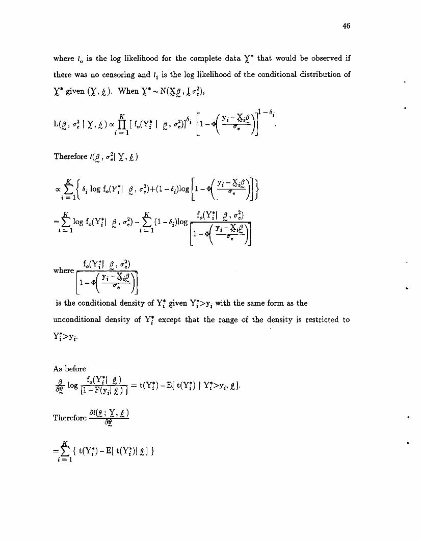
Recall that the likelihood function for the observed data (y, £) can be expressed as
where 10
is the log likelihood for the complete data Y* that would be observed if
there was no censoring and 11 is the log likelihood of the conditional distribution of
Y* given (y, £).
When Y* ,.., N(~e ' 10";),
Therefore I(e ' 0";1 Y, £)
is the conditional density of Yi given Yi>ci with the same form as the
unconditional density of Yi except that the range of the density is restricted to

26
I
As before
o fo(Yil f) - (Y*) E[ (Y*) I Y* ]of log [1 _ F(cil f ) ] - t i - t i i >Ci' f 0
Th £0/(0 ; Y, 0 )
ere ore "'" "'" "'"00"'"
K=2: {t(yn- E[ t(ynl f] }i=l
K- 2: (1- 0i){ t(Yi) - E[ t(Yi) I Yi>ci' f] }i=l
K=2: {E[ t(Yi) I y=y, f., f] -E[ t(Ynl f] }
i =1 "'"
the difference between the conditional and unconditional expectations of the
complete-data sufficient statistics and when fb. =f =E in (1.202) then E is also a
solution of the
10k 10h d 0 0/(0 ; Y, 0) 01 e 1 00 equatIon "'" oi '" "'" 0
•

27
1.2.2.4 EM Computations;General Linear Univariate Models with Fixed Right Censoring
EM Computations are summarized in this section. In the E step, the
conditional expected values of the 'complete-data' sufficient statistic are computed
from the observed data and current estimates of the parameters, while in the M
step, new estimates of the unknown parameters are computed using the conditional
expected values of the 'complete-data' sufficient statistics in the maximum
likelihood equations.
In the r-th iteration, the estimation step computes the conditional expected
values of the complete-data sufficient statistics given the observed data y and the
estimated values of the parameters from the (r - 1)-st iteration. Not all of the Y*
are observed so the E step will estimate the complete-data sufficient statistics that
involve Y*.'"
A set of complete-data sufficient statistics for this problem is
X'Y* and y*'y*.f"oJ ""J "..."...
The expected values of the complete-data sufficient statistics may be denoted,
t (r)=x, E[Y* I Y 6 {3(r -1) er(r _1)2] and,.."" 1 "... f/'IoJ ,..",.' N' N 'e
When 6i=0 expectations involving the i-th element of the complete-data sufficient
statistics can be computed as:
E[Y'!' I Y·=c· 6.=0 {3(r-l) (r_l)2]J J J' J '", ' ere

28
=E[Y! IY!>c. /3(r-1) (r_1)2]I I I' .... ,Ue
c.-X ./3(r-1)where z(r -1) I .... I ....
I (r -1)Ue
and
E[y!2 I y.=y. c.=0 a(r -1) (r _1)2]I I I' I ' ~ , Ue
Both of these expectations appear in Aitkin (1981).
M~:
The r-th iteration of the M step obtains ~ (r) and u~r)2 as solution to equation
1.2.3. For the complete-data problem the maximum likelihood estimates are:
e=(~'~) -1 ~'Y*
and
..
..

29
Initial values of maxImum likelihood estimates are obtained by treating the
censored data as if they were uncensored. Convenient initial estimates are:
e(O)=(~'~) -1 ~'Y
and
u(0)2=.l.(y _ Xp(O»)'(y _ XP(O»).e K "'J "'J"", ,...,,...,,....,
In the r-th iteration maximum likelihood estimates which maximize the likelihood
function using the expected values of the complete-data sufficient statistics
obtained from the previous iteration of the E step are:
and
u(r)2=.l.[t (r) _ 2p(r -1)' t (r)+p(r -1)'X'xp(r -1)].e K 2 N N 1 N N NN

30
1.2.3 Mixed Models with Noninformative Right Censoringor Fixed Left Censoring
Consider a random sample of K individuals with ni observations for the i-thK
subject such that n= I: ni. The n observations are assumed to be a sample from ai=l
normal population with common parameters f3, D, and O'~. The General Linear"" ""
Mixed Model is
(1.2.4)
where
Xi is an ni x 1 vector of failure values which mayor may not be observed,
~i is an ni x p known constant matrix of rank r::; p,
f3 is a p x 1 vector of unknown constant 'fixed' population parameters,""~i is an ni x q known matrix corresponding to the random effects,
2i is a q x 1 vector of unknown individual parameters,
~ i is an ni x 1 vector of unobservable random errors ,
2i ,.., N(Q , R) independent of ~ i"" N(Q, 1nt~)'
:g is a positive-definite symmetric q x q covariance matrix of
random effects,2 i'
and O'~ is an unknown within-subject variance component.
Therefore Xi,.., N(~i~' ~ i)' each with marginal density
..
x exp [-k- (Y~-X'f3)' (E.)-l(Y~-X'f3)]~ ~I ~I~ ~Z ~I ~I~
and log likelihood of the complete data subvector Xi
lo(~ , ~ i I Xi)=log fo(Xi I ~,~ i)

31
=- ~i log(211")-~logl~il-~ [(ri-!ie)' (~i)-l(ri-!i~)]
where ~ i=~ iI:?~ i+! nl"~
is the positive-definite symmetric covariance matrix of Xi.Note that X* denotes the complete data vector in the absence of censoring.
Similarly let Qi-Hi2 +~ i'X i+!i,
where
Qi is an ni x 1 vector of censoring values which mayor may not be observed,
tli is an ni x Ph known constant matrix of rank rh ~ Ph,
2 is a Ph x 1 vector of unknown constant 'fixed' population parameters,
~i is an ni x qh known matrix corresponding to the random effects,
'X i is a qh x 1 vector of unknown individual parameters,
£ i is an ni x 1 vector of unobservable random errors,
'X i ...... N(Q, y) independent of £ i ...... N(Q,! nl"~)'
y is a positive-definite symmetric qh x qh covariance matrix of
random effects, 'X i'
and O'~ is an unknown within-subject variance component.
Therefore Qi...... N(tli2 , I i)
with densityni 1
* [1]2--g (C· I Q r .)= - I r·1 2o '" 2 '" , '" 2 211" '" Z
and log likelihood
10 (2, I i I Qi)=log go(Qi I 2, I i)
x exp [-~ (C'!' - H'Q)' (r.) -l(C'!' - H·Q )J4, N I N Z""""" ......,Z N Z !"'oJ z..;;;;.

Define:
32
where r ;=J ;VJ ~+I n.O'~f!'oJ. I'"V."'" ,..,.". f'IW I 'I;.
is the positive-definite symmetric covariance matrix of Qi.
y .. =min(Y!· C!·)I) I)' I)
{, ..=c:B(y ..= Y! .)I) I) I)
where c:B is the Boolean function (Helms 1988) and let ~ i denote the vector of
indicator variables for non-right censoring in the i-th individual, where right
censoring occurs when the log censoring time Cij is less than the log survival time
Yij'
Pettitt (1985) assumes that censoring is noninformative, i.e. that
1. Xi and Qi and independent and
2. Parameters of the distribution of Xi are functionally independent of the
parameters of the distribution of Qiand defines the likelihood used to obtain maximum likelihood estimates of /3, D,
'" '"
and O'~ to be
L(~ , ~, O'~ I X)= II Li(~ , ~, O'~ IXi)i = 1
where
and e denotes the set of mIssmg or right censored observations in XiAlternatively, after partitioning Xi into an observed data vector (X i) and a
missing data vector (¥i) (Carriquiry 1985), the likelihood function for the i-th
individual can be written in more compact notation as

33
Pettitt (1985) solved this problem usmg the EM Algorithm. Using his
approach it is necessary to estimate the random effects (2 i) in the E step. As a
result the complete-data sufficient statistics involve functions of r i and 2i and
expected values of the complete-data sufficient statistics are computed given {3, D,- -and IT~ but not 2i'
and consequently the r i are not conditionally independent.
Some of the complete-data sufficient statistics involve functions of y!. Given_l
e' .Q, IT~ the expectations of yij and YijYik are
(1.2.5)
and
where the denominator of (1.2.5) is the likelihood of the observed data.
Consequently, using Pettitt's approach, in order to obtain the expected values
34
of the complete-data sufficient statistics which are functions of r i it is often
necessary to carry out high-dimensional integrations. This is computationally
infeasible for many real-data problems.
A mixed model procedure for the analysis of multivariate normal survival data
using a Bayesian approach was developed by Carriquiry (1985) and Carriquiry et
al. (1987). They described how to estimate fixed effects and variance components
for a random intercept model when records were left censored at time c, a
predetermined fixed constant. Unlike Pettitt (1985) they estimated the random
effects as well as fixed effects. Given a random sample of K individuals with nj
Kobservations for the i'th individual such that n= L nj, the n observations are
j =1
assumed to be a sample from a normal distribution with common parameters /3 , D,..... .....
and O'~.
Stacking the ri matrices defined in (1.2.4), let
Y* = ~e + ~Q + ~,
where
Y* is an n x 1 vector of failure values which mayor may not be observed,
~ is an n x p known constant matrix of rank r:5 p,
/3 is a p x 1 vector of unknown constant 'fixed' population parameters,.....
~ is an n x Kq known block-diagonal design matrix corresponding to
the random effects,
Q is a Kq x 1 vector of unknown individual parameters,
~ is an n x 1 vector of unobservable random errors,
Q- N(Q, ~O'~) independent of ~ - N(Q, ! O'~),
~ is a positive-definite symmetric Kq x Kq covariance matrix,
and O'~ and O'~ are the unknown between- and within-subject variance components.
Therefore

35
where
~ = ~ ~~/cT~ +1ncT~
is the positive-definite symmetric covariance matrix of y.
For a given individual
y:t'=x .,I3+B. d· +e., i=1, ... ,K,'" 1 '" z'" '" z '" z '" 1
Carriquiry et al. (1987) suggest conditioning on both the fixed and random effects
so that
and the elements of (Y* Ie, g) are conditionally independent, eliminating the
need to compute multi-dimensional integrals.
The likelihood function can be simplified by partitioning Y into a vector of n l
uncensored observations and n2 censored observations,
Y*= [~n'
The likelihood of the conditional distribution of O~ 1 Ie, g) is:
while, for censored observations,
where
and
/)(Zl) is the probability of the I-th observation being left censored at c.
(1.2.6)

36
Thereforen
Pr(Y2n+1<c'''.'Y2n<cle,2,1T~)= II ~(zl), 1 ' l=nl+1
(1.2.7)
which is the joint probability of all observations in Y2 being left censored. The
product of (1.2.6) and (1.2.7) gives the likelihood function for the whole sample
(Carriquiry 1985, Carriquiryet al. 1987):
- [ 1 J~l- 211"IT; x (1.2.8)
Prior Distributions:
Unlike the mixed model approach where e is assumed fixed, the Bayesian
approach assumes that all parameters are random variables. Harville (1974, 1976,
1977) shows that restricted maximum likelihood estimation of variance components
is equivalent to Bayesian procedures with flat priors for e and the components of
IT~ using all the data. Suitable prior distributions for this problem are:
III (f3)ex: constant,-II2(2 I IT~) = N Kq(Q, ~IT~), and
II3(IT~, IT;) ex: constant.
This leads to the joint prior distribution
II(e ' 2, IT~, IT;) ex: III (e) . II2(2 I IT~) . II3( IT~, IT;)
Posterior Distribution:
(1.2.9)
The joint distribution of t, i, e, 2, IT~, and IT~ is equal to the product of the
37
conditional likelihood in (1.2.8) and the joint prior distribution in (1.2.9), i.e.
p(r, .e, edL (T~, (T~)=f(r ,.e IedL (T~, (T~) x II(e, Q, (T~, (T~) .
Using Bayes Theorem
p(.B , d, (T~, (T~ I Y, 6 )f"tJ "V f"tJ f"tJ
p(y, .e , e'Q, (T~, (T~)
p(Y, 6 , .B, Q, (T~, (T~)_ ,.. f/IItJ N
- p(Y,.e )
Since p(r,.e ) does not depend on any of the parameters, maximizing p(e, Q, (T~,
(T~ I Y,.e ) is equivalent to maximizing p(Y, .e, e, Q, (T~, (T~) with respect to e, Q,2 2(Td' or (Te'
Therefore the posterior distribution of e, Q, (T~, and (T~ IS
p(Y, .e , e'Q, (T~, (T~)
p(Y, .e)

38
(1.2.10)
It is usually not practical to perform the integrations needed to obtain
parameter estimates from (1.2.10) directly. Instead Carriquiry (1985) and
Carriquiry et al. (1987) developed an iterative approach using the Newton
Raphson algorithm to obtain estimates of fixed and random effects assuming
variances were known and then used these to estimate variance components. This
involved estimating the posterior modes or maximum a posteriori values of /3 and.....
2 of the joint posterior distribution in equation 1.2.10 using a procedure that is
referred to as "maximum a posteriori" estimation (Beck and Arnold 1977) which
can be viewed as a Bayesian extension of maximum likelihood estimation.
Posterior mode estimators are equivalent to maximum likelihood estimates for
parameters with flat priors (Laird and Ware 1982), but in this case we do not have
flat priors for the random effects.
Newton-Raphson algorithm:
Let L(/3 , d )=log p(/3, d, O'~, O'~ I Y, 0). The Newton-Raphson algorithm is used to""'J ,..." !"'oJ ,..." ,..." ,..."
obtain estimates of /3 and d where..... .....
+a/3 a/3 ',... ,...
ad a/3',... ,...
a/3 ad',... ,...
ad ad ',... ,...

xL({3, d)
'" '"8{3
8L(£, 2)82
39
For large samples, this requires the inversion of very large matrices of the order of
the number of subjects in order to obtain estimates of fixed and random effects.

40.
1.3 Statement of the problem and outline
The mixed model procedures described in Section 1.2.3 are summarized in
Table 1.3.1. The use of the EM algorithm is often preferable to gradient methods
(e.g., Newton-Raphson algorithm, Method of Scoring) when maximum likelihood
solutions are more easily obtained for the likelihood of the complete data
conditional on the observed data than for the likelihood of the observed data alone.
The likelihood of the complete data for the General Linear Mixed Model has a
much simpler form than the likelihood corresponding to the General Linear Mixed
Model with censored data. Using the EM algorithm, computations involved in
obtaining parameter estimates in the M step are straightforward. However, using
Pettitt's (1985) approach, computations in the E-step involving estimation of the
random effects and censored data can involve high-dimensional integrations when
censoring occurs.
This was not a problem for Carriquiry et al. (1987) because they used an
extension of maximum likelihood estimation known as maximum a posteriori
estimation. However, using this approach in conjunction with the Newton-Raphson
algorithm other complications arose because parameter estimates had to be
obtained using the likelihood of the observed data. Although they eliminated the
difficulty of having to perform high-dimensional integrations this was offset by the
fact that their method required the inversion of very large matrices, of the order of
the number of subjects, in order to obtain estimates of fixed and random effects.
For example, it would be necessary to invert a 41 x 41 matrix to estimate the
fixed and random effects in the example from Wei, Lin, and Weissfeld (1989)
described in Section 1.1. In this example, there were only 36 patients. If there had
been ten times as many patients, the dimension of the matrix would be 365 x 365.

41
Similarly, for 1000 patients, it would be necessary to invert a 1005 x 1005 matrix.
However, in the M-step of the EM algorithm the dimensions of the matrices
required to estimate fixed and random effects would always be 5 x 5 and 1 x 1,
respectively, for each subject regardless how many subjects there were.
Carriquiry, Gianola, and Fernando's (1987) method was also restricted to
random intercept models. In fact, if they had attempted to fit a model with a
random intercept and a random slope, the dimension of the matrices they would
have to invert would be almost double the dimensions for the random intercept
model.
The approach taken in this dissertation IS to use maxImum a posteriori
estimation instead of maximum likelihood estimation in order to avoid the problem
of having to compute high-dimensional integrals and to use the EM algorithm
instead of the Newton-Raphson algorithm. This approach takes full advantage of
the simple computational form of the likelihood for the complete data and avoids
having to invert large matrices.
Unlike Pettitt's (1985) approach, the EM algorithm for noninformative right
censoring proposed in Section 3.1 uses maximum a posteriori estimation to obtain
parameter estimates of the random effects in the M-step, eliminating the need to
compute multi-dimensional integrations in the E-step. This is because
expectations involving the responses for the i-th individual are conditionally
independent given estimates of both fixed and random effects.
This approach is also not restricted to study designs with fixed or
noninformative random censonng. The approach developed in Section 3.1 for
noninformative random censoring mechanisms will be extended to informative
censoring in Section 3.2.

TABLE 1.3.1SUMMARY OF MIXED MODEL PROCEDURES
42
PETTITT CARRIQUIRY et al. PROPOSEDPARAMETER ESTIMATION (1985) (1987) METHOD
Maximum Likelihood Estimation X
Maximum a Posteriori Estimation X X
COMPUTATIONAL ALGORITHM
EM Algorithm X X
Newton-Raphson Algorithm X
TYPE OF CENSORING
Fixed Censoring X X
Noninformative Random Censoring X X
Informative Censoring X
LIMITATIONS
High-Dimensional Integrations X
Inversion of Large Matrices X
Restricted to RandomIntercept Models X

TABLE 1.3.2
DIMENSIONS OF MATRICES THAT MUSTBE INVERTED IN ORDER TO ESTIMATEFIXED AND RANDOM EFFECTS
43
Fixed Random Pettitt (1985) and Proposed MethodEffects Effects Carriquiry et al. 1 Fixed Random
(#) (#) (1987) Effects Effects
5 36 41 x 41 5 x 5 1 x 15 360 365 x 365 5 x 5 1 x 15 1000 1005 x 1005 5 x 5 1 x 1
1. Carriquiryet al. (1987) estimate fixed and random effects simultaneously.

44
ll. GENERAL LINEAR UNIVABlATE MODELSWITH RANDOM CENSORING
The Cox and Oakes (1984) method assumes that the censormg values are
predetermined constants (ci) that are known to the investigator in advance. In
practice the ci usually are not known in advance and cannot be treated as fixed
constants. In this chapter the Cox and Oakes (1984) method is extended to
random noninformative right censoring in Section 2.1 and further extended to
informative censoring in Section 2.2.
2.1 General Linear Univariate Models with Noninformative Right Censoring
In Section 2.1.1 the EM algorithm is derived for the general linear univariate
model with noninformative right censoring. Corresponding EM Computations are
described in Section 2.1.2.
2.1.1 General Linear Univariate Models with Noninformative Right Censoring;Derivation of the EM Algorithm
The method of Cox and Oakes (1984) described in Section 1.2.2.3 can easily be
extended to noninformative right censoring. In the expectation step,
E[ t(Yi) IYi=Yi' ci' f J=
ciE[ t(Yi) I Yi=Yi, ci=l, f ]+(1- ci)E[ t(Yi) I Yi=Yi' ci=O, f]
..

45
with corresponding density function
!o(Y* I Y*>y)=!o(Y* I Y=y, 6=0)
fo(Y*=y*, Y=y, 6=0)fo( Y=y, 6=0)
fo(Y*=y*, C*=y)00Jfo(Y*, C*) dY*y
The last step follows from an argument analogous to the one in Section 1.1.
If y* and C* are independent,
fo(Y* I Y*>y) 00
gC*(y) Jfo(Y*) dY*y
Therefore
Recall that the likelihood function for the observed data ex, §.) can be expressed as
46
where 10
is the log likelihood for the complete data Y* that would be observed if
there was no censoring and 11 is the log likelihood of the conditional distribution of
Y* given (Y, ~). When Y* "" N(~e ' ! u;),
Therefore I(e ' u~1 Y, ~ )
where
is the conditional density of Yi given Yi>Yi with the same form as the
unconditional density of Yi except that the range of the density is restricted to
Yi>Yi·
As before
o I fo(Yil f) - (Y*) E[ (Y*) I y* ]of og [1- F(yil f) ] - t i - t i i >Yi' f .
Th £01(0; Y, a)
ere ore '" '" '"00'"
K= L: { t(Yi) -E[ t(Yi)1 f] }
i = 1

47
K= L {E[ t(Yi) I Y=y , §. , f] - E[ t(Vi) If] }i=l ""
the difference between the conditional and unconditional expectations of the
complete-data sufficient statistics and when fI=f =l in (1.2.2) then l is also a
solution of the
10k l"h d . 8l( (J ; V, 8) 01 e 1 00 equatIOn "" G(J"" "" "" 0
""

48
2.1.2 General Linear Univariate Models with Noninfonnative Right Censoring;
EM Computations
EM Computations are summarized in this section. In the E step, the
conditional expected values of the 'complete-data' sufficient statistic are computed
from the observed data and current estimates of the parameters, while in the M
step, new estimates of the unknown parameters are computed using the conditional
expected values of the 'complete-data' sufficient statistics in the maximum
likelihood equations.
In the r-th iteration, the estimation step computes the conditional expected
values of the complete-data sufficient statistics given the observed data y and the
estimated values of the parameters from the (r -l)-st iteration. Not all of the Y*
are observed so the E step will estimate the complete-data sufficient statistics that
involve Y*.N
A set of complete-data sufficient statistics for this problem is
X'Y* and y*'Y*.f"tJ 1"tJ 1"tJ 1"tJ
The expected values of the complete-data sufficient statistics may be denoted,
t (r)=x, E[Y* I Y 0 /3(r -1) (7'(r _1)2] and,...",1 1"tJ ,...", ,.."" , ,..", , '""'" 'e
t (r)=E[Y*'y* I Y 0 /3(r -1) (7'(r _1)2].2 1"tJ 1"tJ ........ ' """" 1"tJ 'e
When 0i=O expectations involving the i-th element of the complete-data sufficient
statistics can be computed as:
E[Y'!' I y.=y. 0.=0 /3(r-1) (r_1)2]l l l' l 'N ' (7'e
..
..
•

49
=E[Y'!' I Y'!'>y. j3(r-1) (r_1)2]a a a'_ ,(7e
y._X.j3(r-1)where z(r -1) a ..... a.....
a (r-1)(7e
and
E[y,!,21Y.=y. 0.=0 j3(r-1) (r_1)2]
a a a' a '..... ' (7e
M~:
The r-th iteration of the M step obtains j3 (r) and (7~r)2 as the solution to-equation 1.2.3. For the complete-data problem the maximum likelihood estimates
are:
jj =(X'X) -1 X'Y·f'OW ~ N f"t.J f'O<.I
and

50
Initial values of maxImum likelihood estimates are obtained by treating the
censored data as if they were uncensored. Convenient initial estimates are:
e(O)=(~'~) -1 ~'Y
and
q(0)2=~(y _ X.a(O»)'(y _ X.a(O»)e E. N NN N N,oy
In the r-th iteration maximum likelihood estimates which maximize the likelihood
function using the expected values of the complete-data sufficient statistics
obtained from the previous iteration of the E step are:
and
q(r)2=..!.[t (r) _ 2.a(r -1)' t (r)+.a(r -I)'X'x.a(r -1)].e K 2 _ _1 _ _ __
•

51
2.2 General Linear Univariate Models with Informative Right Censoring
In Section 2.2.1 the EM algorithm is derived for the general linear univariate
model with informative right censormg. Corresponding EM Computations are
described in Section 2.2.2.
2.2.1 General Linear Univariate Models with Informative Right Censoring;Derivation of the EM Algorithm
Consider a random sample of K individuals with one observation per subject from a
normal population with common parameters I' G, and n. The General LinearN N N
Univariate Model is
w*=[Y*~ =[ ~N C* 0.... ....
where
Vj* is a 2n x 1 vector of failure and censoring values which mayor may not
be observed,
~=[ ~ ~] is a 2n x2p known constant matrix of rank 2r S; 2p,
z=[ ;] is a 2p x 1 vector of nnknown constant 'fixed' popnlation parameters,
£ =[~] is a 2n x 1 vector of nnobservable random errors,

52
consists of the unknown within-subject
variance components, where
Q 01n=
Define: 81i=G.B(Yi=Yi), 82i=G.B(Ci=Ci),
and W to be the observed values of W*,- -where G.B is the Boolean function (Helms 1988).
The joint bivariate normal distribution of the complete-data vector,
Vj*.... N( ~Z' Q 01 )
with densityK
fo(Vj* IZ' n)= [2~] K IQ 1-"2 x exp [- t- (Vj* - ~Z)' (Q -1 01) (Vj* - ~1)]
and log likelihood
=-K log(211")-~ logl Q I-~ [(Vj*-~Z)' (Q -1 0 1) (Vj*-~l)]
is a member of the exponential class of distributions. The density has the regular
exponential-family form
fo(Vj*1 f!. )=b(Vj*) exp [ f!.' t(Vj*) ] / a(f!.) and •

53
=t(W*) - E[ t(W*) If]·
where f ={e, u;, 2, u;, p} denotes the parameter vector that is restricted to a
(p+1)-dimensional convex set! such that fo(W*1 f) defines a density for all f III
! and
a(f)=Jb(W*) exp [ f' t(W*)] dW*w*
where w* is the sample space of W*.""
For a right censored sample (W, ~) the function
Q(ft, f )=E[/o(f1 I W*) I W, ~, f]
=E[ ~t(W*) -log a(ft) I W, ~,f]+log b(W*)
=E[ f~t(W*) I W, ~,f] -log a(ft)+log b(W*)·
For a concave function 10 , Q is maximized with respect to f1 when
o aQ(f1' f) E[ t(W*) I W 8 ()] _ alog a(ft)aft "" "" , "" , "" af1
=E[ t(W*) I W, ~, f] - E[ t(W*) I f1]
or E[ t(W*) I W, ~,f]=E[ t(W*) I f1]·
The corresponding E and M steps are:
E-step: Compute t(r)(W*)=E[ t(W*) I VI, ~, f(r -1)]
M-step: Obtain f(r)as the solution to E[ t(\'y*) I f(r)]=t(r)(\'y*). (2.2.1)

54
With bivariate right censoring, there are three cases to be considered:
(1) 61i=62i=1, i.e., both Yi and Ci are known,
(2) 61i=1 and 62i=0 which implies that Ci>Yi=Yi
and (3) 61i=0 and 62i=1 which implies that Yi>Ci=C i.
It is assumed that at least one of the Y i or Ci is observed. If both are missing (i.e.,
61i=62i=0), this observation is assumed to be ignorably missing.
In the expectation step,
E[ t(W'f) I W·=w· 6· BJ=z z z' "'z' '"
6li62iE[ t(Wnl Wi=wi' 6li=1, 62i=1, .eJ
+(1-6li)62iE[ t(Wi) I Wi=wi, 61i=0, 62i=1, .eJ
+61i(1- 62i)E[ t(Wi) IWi=wi' 61i=1, 62i=0, .e J
=61i62iE[ t(Wi)1 Wi=wi' .e J
+(1- 61i)62iE[ t(Wn IYi>Yi, Ci=Yi, .e J
+61i(1 - 62i)E[ t(Wi) I Yi=Yi' Ci>Yi' .e J
=61i62it(Wi)
+(1- 61i)62iE[ t(Wi) I Yi>Yi' Ci=Yi' .e J
+61i(1- 62i)E[ t(Wi) I Yi=Yi' Ci>Yi' .e J
with corresponding density functions
•

fo(Y*=y*, Y=y, °1=0, °2=1)fo( Y=y, 01 =0, 02=1)
00
gC*(y) Jfo(Y*1 C*=y) dY*y
fo(Y*=y*, C*=y)00Jfo(Y*, C*) dY*y
55
00Jfo(Y*1 C*=y) dY*y
fo(Y*1 C*=y)1- 4>(Zy* Ic*)
where Zy* Ic*, i
Similarly,
fo(C*=c*, Y=y, °1=1, 02=0)
fo( Y=y, °1=.1, °2=0)
00
fy*(y) Jgo(C*1 y*=y) dC*y
fo(y*=y, C*=c*)00Jfo(Y*, C*) dC*y
00Jgo(C*1 y*=y) dC*y
go(C*1 y*=y)1- 4>(zc* Iy*)
..where zc* IY*, i

Therefore
00
1- ~(Z;'IC" ;) I. t(Wi) f.(Yi I Ci=Yi, f) dYi
and
00
1-~(Z:'I y', ,) I. t(Wi) g.(C; IYi=Yi, f) dC;'
56
..
•

..
57
2.2.2 General Linear Univariate Models with Informative Right Censoring;
EM Computations
EM Computations are summarized in this section. In the E step, the
conditional expected values of the 'complete-data' sufficient statistic are computed
from the observed data and current estimates of the parameters, while in the M
step, new estimates of the unknown parameters are computed using the conditional
expected values of the 'complete-data' sufficient statistics in the maximum
likelihood equations.
In the r-th iteration, the estimation step computes the conditional expected
values of the complete-data sufficient statistics given the observed data Vj and the
estimated values of the parameters from the (r -1 )-st iteration. Not all of the Vj*
are observed so the E step will estimate the complete-data sufficient statistics that
involve W*.'"
A set of complete-data sufficient statistics for this problem is
The r-th iteration of the E-step consists of evaluating the expectations:
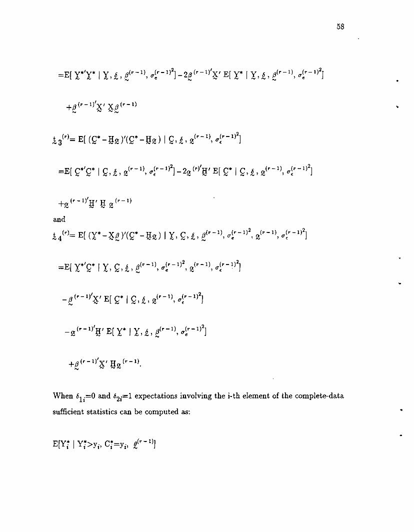
58
and
t (r)= E[ (Y*-X/3)'(C*-Ha) I Y C 6 /3(r-I) q(r_I)2 a(r-I) q(r-1)2]"",,4 "'V Nf'OV """ NI'oJ """',..,,,' """,' ""'" 'e '""" ,(
When 61i=O and 62i=1 expectations involving the i-th element of the complete-data
sufficient statistics can be computed as:
E[Y* I Y* C*- l1(r -1)]i i>Yi' i-Yi'!?'

.'
59
00 f (Y*I C*- (r -I»)=/ Y! 0 i i-Yi' f dY!t 1 ((r-I») t
Yi - ~ Zy. Ic·, i
where
(r -I)zY·1 c·, i
"
and
00 f (Y*I C*- (r -I»)=/ y!2 0 i i-Yi' f dY!t 1-~( (r-I).) I
Yi Zy·,c·, t
1 (r -I)
+ ue(r-I)(1_p(r-I)2)2 x [y+X,/.1(r-I)+ (r-I)ue (y._H.a(r-I»)]
t - t~ P (r - I) t _ t_U
f
( (r-I) )t/J zY·1 c·, i
x 1 ....( (r -I) )'- 'j<' zY·1 c·, i
Similarly, when 0li=l and 02i=O expectations involving the i-th element of the
complete-data sufficient statistics can be computed as:

E[C* IY*- C* lI(r -1)]i i-Yi' i>Yi' ~
00 (C*I Y*_ (r -1))=j C! go i i-Yi' R., dC!J 1 ((r-l)) J
Yi - cI) Zc· IY·, i
where
( (r-l) )t/J ZC·' Y·, i
1 cI)( (r-l) )- ZC·' Y·, i
60
..
(r -1)ZC·' Y·, i
and
00 (C*I Y*_ (r -1))=j C~2 go i i-Yi' R., dC!J 1 ((r-l)) J
Yi - cI) ZC· IY·, i
...
..
t/J(z~·1 ~., i)x 1 ((r - 1) )'
- cI) ZC· IY·, i

.'
.'
61
M~:
The r-th iteration of the M step obtains j3 (r), 0: (r), 0'~r)2, 0'~r)2, and p(r) as the"" ""
solution to equation 2.2.1. For the complete-data problem the maximum likelihood
estimates are:
U2=.l.(C* - H5 )'(C* - H5)(: K "'V "...,,,..., "oJ "...,,,...,'
and
P=K1 ~ (Y*-XP)'(C*-H5).l7e(j (:"..., "..., N N N ,...,
Initial values of maxImum likelihood estimates are obtained by treating the
censored data as if they were uncensored. Convenient initial estimates are:
0'(0)2=.l.(C _ Ho:(O»)'(C _ Ho:(O»)(: K"...,,,...,""'J "'oJ"""""" ,
and
p(O) K (~) (O)(Y - ~£(O»)'(g - tl2(O»).O'e O'f

62
In the r-th iteration maximum likelihood estimates which maximize the likelihood
function using the expected values of the complete-data sufficient statistics
obtained from the previous iteration of the E step are:
and
p(r) 1 t (r)
E., (r-l) (r-l) 4<1'e <1'(
..

"
.'
63
ill. MIXED MODELS WITH RANDOM CENSORING
In this chapter, the methods discussed in Chapter 2 for general linear
univariate models with random censoring are extended to mixed models with
noninformative censoring in discussed In Section 3.1 and extended further to
informative censoring in Section 3.2.
3.1 Mixed Models with Noninformative Right Censoring.
Likelihood functions for complete data are derived in Section 3.1.1, and theory
and applications of the EM algorithm to mixed models with random
noninformative right censoring are discussed in Sections 3.1.2 and 3.1.3.
3.1.1 Mixed Models with Noninformative Right Censoring; Likelihood Functions
If there is no censoring, the probability density function (pdf) of r * given f3""
and 2. IS:
f(Y*1 ~, 2., O"~)
K=II f(Yf I ~ , 2. i' O"~)i=l

64
K ni=II [_1_]2 x exp[-lr[(Y~-X'/3-B.d.)/((72In.)-I(Y~-X'/3-B.d.)] ]
2 2 " "'1 "'1", "'1"'1 e", I "'1 "'1", "'1"'1i = 1 1r(7e
_ [ 1 ]~- 21r(7~
x exp --21 [f. [(Y~-X'/3-B.d.)/((72In.)-I(Y~-X'/3-B'd')]].L-i ""'J 1 ""J 1""""", I"V 11"'\,1 1 e ""'J I ~ I """J '"""" """" I f"IoJ I
J = 1(3.1.1)
..
Suitable flat prior distributions for this problem are:
ITl(~) ex constant, and
IT2(Q, (7~) ex constant,
and a convenient prior for!! i is
This leads to the joint prior distributionK
IT(~, !!, 12, (7~) ex ITl(~) . II IT3 (!! i /12) . IT2(Q, (7~).i = 1
(3.1.2)
The joint p.d.f. of the distribution of Y*, /3 , d, D, and (7~ is equal to the product ofI'tW I"V """J N
the conditional density in (3.1.1) and the joint prior distribution in (3.1.2), i.e.
p(Y*, /3 , d, D, (7~)=f(Y* I /3 , d, D, (7~) x IT(/3, d, D, (7~) ."""" """" """" ,..., ""J ""oJ ,..., I"V """" f'OoJ ""'J
Using Bayes Theorem
p(/3 , d, D, (7~ I Y*)I"V fI'ItJ "'J """"
p(Y*, /3, d, D, (7~)_ ,...., """" ,..., f"IV
- p(r*)
p(Y*, /3 , d, D, O'~)"""" "J """" """"
"
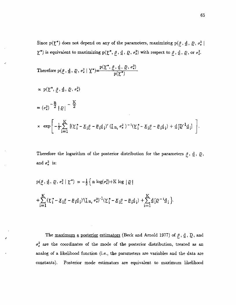
65
Since p(r*) does not depend on any of the parameters, maximizing p(e ' Q, Q, 0"; Iy*) is equivalent to maximizing p(Y*, /3, d, D, 0";) with respect to /3, d, D, or 0";.~ NNNN NNN
x exp [-~~ [(Y~-X'/3 -B.d.)' fIn. 0"2e )-1(Y~-X'/3 -B.d.) + d!D-1d.] ]."L..J -1 -1_ -1-1 u:. , -1 -1_ -1-1 -1--1i=1
Therefore the logarithm of the posterior distribution for the parameters /3, Q, Q,-and 0"; is:
p(e, Q, !2, 0"; I r*) oc -!{n log(O"~)+K log IQI
K K+"'(Y~-X'/3 -B.d.)'fI n . 0"2)-1(Y~_X'/3 -B.d.) +"'d!D- 1d.}.
L..J - 1 -1_ - 1- 1 u:. I e - 1 - 1_ -1- 1 L..J - 1- - 1i=1 i=1
The maximum ~ posterior estimators (Beck and Arnold 1977) of /3 , Q, :Q, and-0"; are the coordinates of the mode of the posterior distribution, treated as an
analog of a likelihood function (i.e., the parameters are variables and the data are
constants). Posterior mode estimators are equivalent to maximum likelihood

66
estimates for parameters with flat priors (Laird and Ware 1982), but in this case
we do not have flat priors for the random effects.
An equivalent derivation using a frequentist approach is given in Fairclough
and Helms (1984) for an artificial General Mixed Model which treats the
unobserved 2/s as missing data, thus facilitating the use of the EM algorithm.
The model is defined as:
The log of the likelihood function can then be written as:
= -!{(n+Kq) log(211')+n log(O'~)+K log 1121
Therefore the posterior distribution of the parameters e, 2, :Q, and 0'; given Y*,
assuming flat priors for fixed effects and variance components and normal priors for
random effects is proportional to the likelihood of e' :Q, and 0'; given Y* and 2 .
Fairclough and Helms (1984) showed that the maximum likelihood estimates of the
parameters f3, d " D, and 0'; are:""J ~ 1 I"V
"
..

."
[K Jl K ~~ = "x!x. " x! (y. - B.d .),'" L...i '" 1 '" 1 L...i '" 1 '" 1 '" 1'" 1
i=1 i=1
mand if 12= L TgQ g then
g=1
~ .lJ t (~-IG ~ -IG ) ]-1 [ ~d~' D~ -IG D~ -1 d~ ]Z; = K\. < race Q '" g 12 '" h >gh <i~ '" i '" '" g '" '" i >g .
67

68
3.1.2 Mixed Models with Noninfonnative Right Censoring;
Derivation of the EM Algorithm
The EM Algorithm (Dempster et al. 1977) can be used to compute maximum
a posteriori estimates of e, 2, !2, and IT~. The distribution of the complete-data
vector,
with density
fo(Y* Ie, 2, ! nlT~)
_[1 ]~- 21l"0'~
x exp [_1 ~ (y! - X ./3 - B ·d .)' a 0'2) -l(y! - X·/3 - B ·d .)]2 ~ _I _ 1_ _ 1_ 1 n e _I _ 1_ _ 1_ 1
i = 1
is a member of the exponential class of distributions. The density has the regular
exponential-family form
fo(Y*1 f )=b(Y*) exp ( f' t(Y*) ] / a(f)
where f ={e, 2, IL IT~} denotes the parameter vector that is restricted to a (p+1)
dimensional convex set ~. Applications of the EM Algorithm to densities from
Regular Exponential Families were discussed in Section 1.2.2.1. The behavior of
the EM Algorithm was previously discussed in Section 1.2.2.2 for the General
Univariate Model. The proof is similar for General Linear Mixed Models except
that f ={e ' 2, 12, O';} instead of {e, O';} and bij=G.B(Yij=Yij) instead of G.B(Yi=Yi).
In addition, the posterior distribution function contains prior information about 2.
For mixed models, the function
the conditional expectation of the logarithm of the posterior distribution function of
•
»

69
Y* given the observed data (Y, .e), where Dij=G.B(Yij= Yij) and Y and.e are
assumed to be fixed and known. Q has two arguments; ft is an argument of the
full likelihood Lo while ft is the parameter of the conditional distribution of Y*
given (r, .e) which is used in computations involving the conditional expectation.
The EM algorithm obtains a value !t* that maximizes f(¥*; ft ).
For this problem the logarithm of the posterior distribution function of ft 1 is
Therefore p(ft I y, .e )=log fo(Y* I ft) -log m(Y* I ¥, .e , ftl)+ log 11"(21 I ~ 1)
=lo(ft, Y*) - ll(ft, Y* I Y, .e)+ log 11"(21 1 ~ 1)
where
Therefore p(ft)=E[ lo(ftl Y*)+log 11"(2 11~1) I ¥,.e, ft] -E[ ll(ftl Y*) I ¥,.e, ft]
=Q(ftl' ft) - R(ftl' ft)
where R(ft, ft )=E[ ll(ftl Y* ) I ¥,.e, ft]·
Consequently,
p(ft) - p(ft )=[Q(ft, ft) - Q{ft , ft)] - [R(ft, ft) - R(ft, ft )].
Using Lemma 1 from Dempster et al. (1977), for any pair (ft, ft) in ~ X ~,
R(ft, ft) ::5 R(ft, ft)· This follows because the expected value of a concave density
function is maximized at the true value of the parameter. Because ft is chosen in

70
the M step to maximize Q(ft, ft) for a previously given value of ft, Q(ft, ft) ~ Q(ft,
ft). Therefore p(ft) - p(ft) ~ 0, so each iteration of the EM algorithm cannot
decrease the posterior distribution function. Note that when the maximum a
posteriori estimator of ft is obtained, the maximum a posteriori estimator, I must
satisfy the self-consistency condition Q(ft, I) $ Q(l, F,), and it is therefore
impossible to increase the value of the posterior distribution function at subsequent
iterations. Note that concavity of Po with respect to the parameters of interest
(e, 2, :Q, and O'~) does not necessarily imply concavity of p.
The method of Cox and Oakes (1984)
noninformative right censoring in mixed models.
exponential class of distributions,
foCY*1 ft )=b(Y*) exp [ !!.' t(Y*) ] / a(ft)·
can easily be extended to
When y* is a member of the.....
For mixed models, Po(ftl Y, t )=log fo(Y, tift) + log 11'(2 I ~) and
oP;~ft) t(Y*) - o~ log a(ft )+o~ log 11'(2 /1J)..... ..... .....
=t(Y*) - E[ t(Y*) I ft]+a~ log 11'(2 I ~)......
For a right censored sample 0::, t) the function
Q(ft, ft )=E[lo(ft I Y*)+log 11'(2 111J I) I Y, t, ft]
=E[ ~ t(Y*) -log a(ft) I Y, ~ , ft ]+log b(Y*)+log 11'(21 11J 1)
=E[ ~t(Y*) I y, ~, ft] -log a(ft)+log b(Y*)+log 11'(21 11Jl)'
For a concave function Po, Q is maximized with respect to ft when
..
..

or
=E[ t(Y*) IY, ~,! l-E[ t(y*) I!11+afllog lI"(Q 1 I th)
E[ t(Y*) I Y, ~ , ! ]=E[ t(Y*) I !J.] - afllog lI"(Q 1 I th)· (3.1.3)
71
The corresponding E and M steps are:
E-step: Compute t (Y*)=E[ t(Y*) I Y, ~ ; !]
M-step: Obtain!1 as the solution to E[ t(Y*) I !J.] - afllog lI"(Q 1 I :Q 1)=t (Y*)·
In the r-th iteration these correspond to:
E-step: Compute t(r)(Y*)=E[ t(Y*) I Y, ~ , !(r -1)]
M-step: Obtain ,e<r)as the solution to
E[ t(Y*) I !(r)] - a(Ja(r) log lI"(Q (r) I :Q(r»)=t(r)(y*).
""
By conditioning on both the fixed and random effects,
In the expectation step,
E[ t(Y!.) I Y..=y.. 6.. (J] =I) I} I}' I}' ""
6. .E[ t(Y!·)1 y ..=y .. 6··=1 (J]+(1-6 ..)E[ t(Y!.) I y ..=y .. 6··=0 ~.]I} I} I} I}' I} , "" I} I}. I} I}' I} '.-
=6· .E[ t(Y!·)1 Y!.=y .. (J ]+(1-6 ..)E[ t(Y!.) I y!.>y .. (J]I) I} I} I}' "" I} I} I} I}' ""
=6· .t(y. ·)+(1-6 ..)E[ t(Y!.) I Y!.>y ..· (J]I) I} I} I} I} I}' ""
with corresponding density function
(3.1.4)

72
fo(Y* I Y*>y)=fo(Y* I Y=y, 6=0)
fo(Y*=y*, Y=y, 6=0)fo( Y=y, 6=0)
fo(Y*=y*, C*=y)00Jfo(Y*' C*) dY*y
The last step follows from an argument analogous to the one in Section 1.1.
If Y* and C* are independent,
fo(Y* I Y*>y) 00
gC*(y) Jfo(Y*) dY*y
Therefore
Recall that the likelihood function for the observed data (Y, §.) can be expressed as
1(&I y, §. )=10 (&, Y*) - 11 (fl' Y* I y, §. )
where 10
is the log likelihood for the complete data Y* that would be observed if
there was no censoring and 11 is the log likelihood of the conditional distribution of
Y* given (Y, §.).
When (Yi' I e, !L)-N(~ie+~i!!i, 10"~),

73
Therefore p(£ ' Q, R, CT~I y, §. )
where [1-~ Yij -iij$. -llij !!;)]is the conditional density of Yij gIven Yij>Yij with the same form as the
unconditional density of Yij except that the range of the density is restricted to
Yij>Yij·

74
As before
Th £ap(o ; Y, 6 )
ere ore - - -ao-
K ni- '" '" (1-6 ..){ t(Y!.) -E[ t(Y!.) I y!.>y .. 0]+ Llog 1r(d·1 D) }L..J.L..J IJ IJ IJ IJ IJ' - ao . - I -i=1 J=1 -I
K=2:
i = 1
n·:t {E[ t(Yij) I Y=~ , §., f] - E[ t(ytj )/ f]+ a~ .log 1r(2 il R) }j = 1 -I
the difference between the conditional and unconditional expectations of the
complete-data sufficient statistics plus the partial derivative of the log prior
distribution for the random effects (2). When b=f =l in (3.1.3) then l is also a
solution of the
. 8p(0; Y, 6)equatIon - at - Q.-

75
3.1.3 Mixed Models with Noninfonnative Right Censoring; EM Computations
EM Computations are summarized in this section. In the E step, the
conditional expected values of the 'complete-data' sufficient statistic are computed
from the observed data and current estimates of the parameters, while in the M
step, new estimates of the unknown parameters are computed using the conditional
expected values of the 'complete-data' sufficient statistics in the maximum a
posteriori estimating equations.
In the r-th iteration, the estimation step computes the conditional expected
values of the complete-data sufficient statistics given the observed data y and the
estimated values of the parameters from the (r - 1)-st iteration. Not all of the Y*
are observed so the E step will estimate the complete-data sufficient statistics that
involve y*. Note that the random individual parameters !L are estimated in the M
step, not the E step. This is in contrast to the usual application of the EM
algorithm for situations where all of the r: are known and complete-data sufficient
statistics involving 2 i are estimated in the E step. By conditioning on both the
fixed and random effects
(ri Ie, 2i) -N(!ie+~i2i,ln/,'~)
and the (ri Ie, 2 i), i=l, 2, ... , N, are conditionally independent, eliminating the
need to compute multi-dimensional integrals.
A set of complete-data sufficient statistics for this problem is
{~iYni =1, n~iYni =If, and {y;'yni =If·

76
The expected values of the complete-data sufficient statistics may be denoted,
t Jr)=x,· E[ V'!' I y. 8. ,a(r-l) d (r-l) n(r-l) 0"(r-l)2].... It .... t .... t .... t' .... t'.... ' .... t '.... 'e
When 8ij=0, Yij>Yij=Cij and expectations involving the (i,j)-th element of the
complete-data sufficient statistics can be computed as:
E[ V'!'· I y ..= .. 8· .=0 Q(r-l) d (r-l) n(r-l) (r_l)2]t) t} Yt}' t} ,~ ' .... t '.... ,0"e
=E[ Y'!'., y'!'.>y.. Q(r-l) d (r-l) n(r-l) (r_l)2]t) t} t}' ~ ' .... t '.... 'O"e
,a(r-l) d (r-l) n(r-l)~ '"""a 'f"oJ ,
1- ct>(z~j-1»)
Y.. _[x ..,a(r-l)+B .. d (r-l)]( 1) t} .... t},... ,... t} ,... t andwhere z r.-t} (r-l) ,
. 0"e
E[ Y'!'7 I y ..=y .. 8 .-0 Q(r-l) d (r-l) n(r-l) 0"(r-l)2]t} t} t}' i}-' ~ ' .... t ',... 'e
=E[ Y'!'7 I y'!'.>y .. ,a(r-l), d (r-l) n(r-l) 0"(r-l)2]t} t} t}',... ,... t ',... , e
•

77
00
=J y'!'~ZJYij
M~:
The r-th iteration of the M step obtains e(rl, 2(r), :g(r), and 0'~r)2 as the
solution to equation 3.1.4. Initial values of maximum a posteriori estimates are
obtained using unweighted regression and by treating censored data as if they were
uncensored. Convenient initial estimates are:
0'(0)2 = 1[~ (y '!' _ X ./3(0)), (y'!' _ X ./3(0))]e n L....J,...",.,.,.,. ,..,.,.,.""" ,
i=1 '" '"
mand if /2= L: O's§ s then
s=1
In the r-th iteration maximum a posteriori estimates which maximize the posterior
distribution function using the expected values of the complete-data sufficient

statistics obtained from the previous iteration of the E step are computed:
mH!2= LTs §s then
s=l
78
•
x
(For details, see Fairclough and Helms 1984).
..

79
3.2 Mixed Models with Informative Right Censoring
Informative censonng is discussed in Section 3.2. Likelihood functions for
complete data are derived in Section 3.2.1, and theory and applications of the EM
algorithm to mixed models with random informative right censoring are discussed
in Sections 3.2.2 and 3.2.3.
3.2.1 Mixed Models with Informative Right Censoring; Likelihood Functions
Consider a random sample of K individuals with ni observations for the i-thK
subject such that n= L ni' The n observations are assumed to be a sample from ai = 1
normal population for which the corresponding the General Linear Mixed Model is
w*=[y*j =[ ~"'" C* 0"'" "'"
where
Vj* is a 2n x 1 vector of failure values and censoring values which mayor may
not
be observed,
A=[ ~"'" Q i ]is a 2n x 2p known constant matrix of rank 2r oS 2p,
z=[ ;] is a 2p x 1 vector of unknown constant 'fixed' population parameters,

random effects,~ ]is a 2n x 2q known matrix corresponding to the
!! = [ ~] is a 2Kq x 1 vector of unobservable individual parameters,
I(i ~] is a 2n x 1 vector of unobservable random errors,
2i"'" N(Q, g) independent of!(. i"'" N(Q, Q 01 n),
9 is a positive-definite symmetric 2q x 2q covariance matrix
of random effects, 2i' and
80
consists of the unknown within-subject
variance components,
...
where
n 01 n.="" "".
and W to be the observed values of W*,"" ""

..
81
where ~ is the Boolean function (Helms 1988).
If there is no censoring, the joint bivariate pdf normal of W* given "( and g IS:- - -f(W* I "( , g , n)
f"'oJ f'oJ t"oJ ,...,.
K= IT f(W: I "( , g i' Q). i=1 - -
K n· _!!=II[.l..J 'Inl 2 x exp [-A(W'1'-A."(-M.g')'(n- 1 @I n .)(W'1'-A."(-M.g.)]21r - .(, - 1 - ,_ -" - -, - 1 - ,_ - '_ '
i=1 -
x exp [_1 .f-. (W'1'-A.,,( -M.g.)'(n- 1 @I n .) (W'1'-A.,,( -M.g.)]. (3.2.1)2.L-J ""'J 1 f'J Z"""" "" Z......, 2......, "" I """" 1 f'oJ 'Z......, ,..., Z"""" Z,= 1
Suitable flat prior distributions for this problem are:
112( g) <X constant,
113 (0-;) <X constant,
114 ( aD <X constant,
IIs(p) <X constant,
and a convenient prior for g i is-116(2 i I g) = Nq(Q, g).
This leads to the joint prior distribution
..(3.2.2)
Let () =b, g, G,f'J f'oJ I"<J f"/oJ
p} denote the parameter vector that is restricted to a

82
(p+1)-dimensional convex set!. The joint p.d.f. of the distribution of Vj* and fl
is equal to the product of the conditional density in (3.2.1) and the joint prior
distribution in (3.2.2), i.e.
p(Vj*, fl )=f(Vj* I fl) x II(fl)·
Using Bayes Theorem
p(fl IVj*)p(Vj*, fl)
Jp(Vj*, fl) dfl().....
p(Vj*, fl)p(Vj*) .
Since p(Vj*) does not depend on any of the parameters, maximizing p(fll Vj*) is
equivalent to maximizing p(Vj*, fl) with respect to fl.
p(Vj*, fl)Therefore p(fll Vj*) p(Vj*) <X p(Vj*, fl )
Therefore the logarithm of the posterior distribution for the parameters -y, g, G,'" '" '"
2 2 d .U'e, U',., an pIS:
p(-y, g, G, U';, U'~, pi W*)f'OW ,..." flOW f"W
<X - ~ { n log Ig 1+K log I9I
..
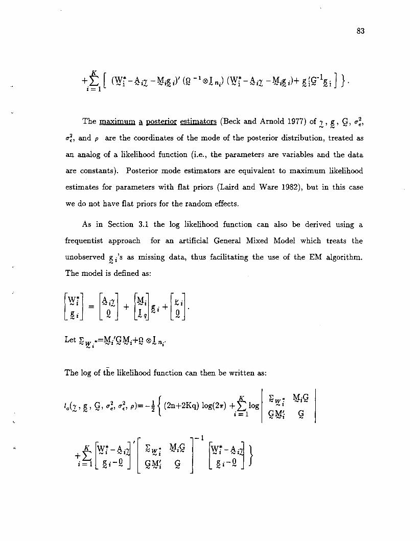
83
+.f-.. [ (W~ -A·'Y -M.g .)' (0 -1@I n.) (W~ -A.'Y -M·g .)+ g !G-1g. ] } ..L...J ~ 1 flOW I,."", f"tJ J"""", Z,..., """'.""'" 1 ,."", Z,."", ,."", %""", 'I ,."",1 ""oJ ,."",1J = 1
The maximum 2 posterior estimators (Beck and Arnold 1977) of '1 , g, g, 0';,- -O'~, and p are the coordinates of the mode of the posterior distribution, treated as
an analog of a likelihood function (i.e., the parameters are variables and the data
are constants). Posterior mode estimators are equivalent to maximum likelihood
estimates for parameters with flat priors (Laird and Ware 1982), but in this case
we do not have flat priors for the random effects.
As in Section 3.1 the log likelihood function can also be derived USIng a
frequentist approach for an artificial General Mixed Model which treats the
unobserved 2/s as missing data, thus facilitating the use of the EM algorithm.
The model is defined as:
Let ~w .*=¥/g¥i+Q @! n;,_,
The log of the likelihood function can then be written as:
GM~_ - J 9
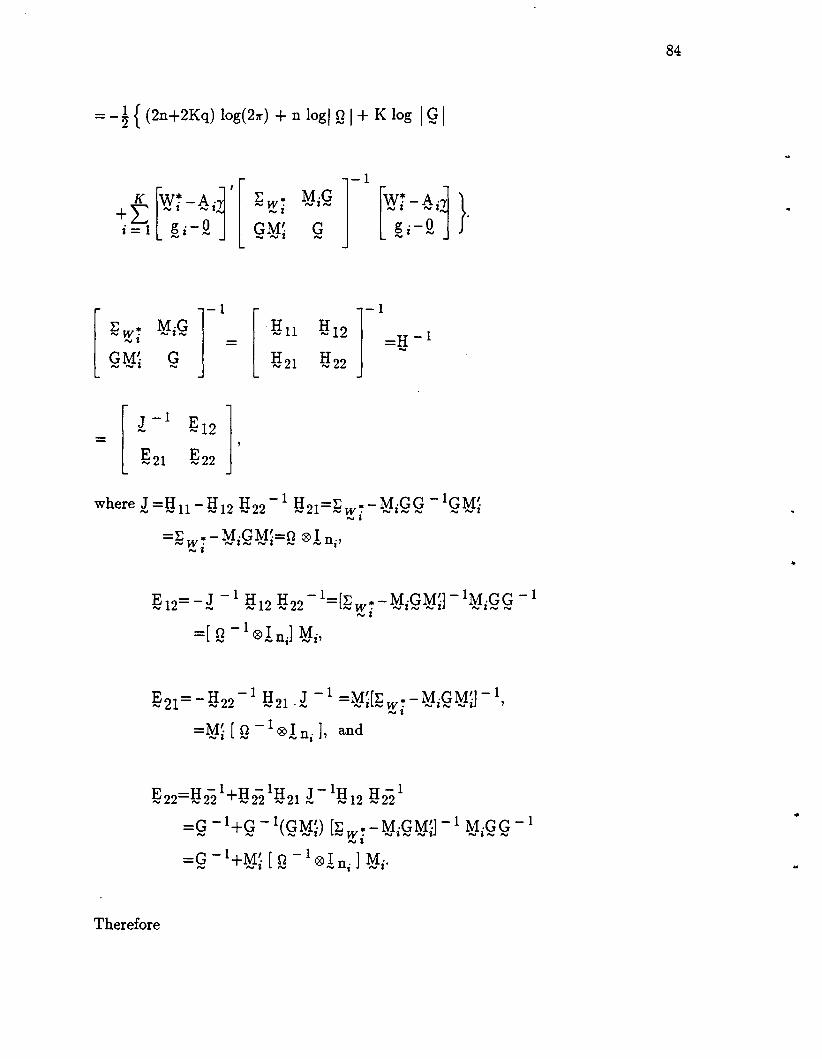
= -!{(2n+2Kq) log(211") + n logIQI+ K log I9 I
84
[
J-1
E ]- .... 12-
~21 ~22 '
where I =tlu - tl12 tl22 -1 tl21=~W~- ¥igg -19¥i_J
=E .-M·GM~=n®I n.,.."" w. ,.,., z......., ,.."., Z ,..." flOW .'_J
E 12=-J -1 H12 H22 - 1=[E *-M.GM~]-1M.GG-1......., #!'oJ ,.."",.."" .......,W. NZ",,,,,,,,Z ,..""z""",,..,,,,
_J
=[ Q - 1 ®! nJ ¥i'
E21=-H22-1 H21 J -1 =M~[E *-M.GM~]-1,,.."" ,.."" ,...,.""W '" Z I"llJ W. ""'" z"""", ,.."., Z
-J
=¥i [Q - 1 ®! ni], and
~22=tl221+tl221tl21I -1tl12 tl22 1
=G -1+G -1(GM~) [E • - M.GM~] -1 M.GG- 1/"OJ ,.."" ,..",.......,Z ,..".,w. ,..""1""",,,,,,,,1 ,..".,1"""",..""
_J
=G -1+MJ~ [ n - 1®In. ] MJ.,""'" ,..,.,,..,,,, ,.."" I "V
Therefore
•
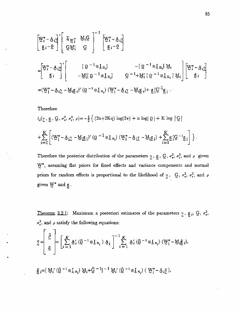
85
[ ~ -1 0 !nJ~ M~[ n - 1 0 1n oj
""'" Z ""'J ""'J I
Therefore
10 (2' ~, g, u;, u~, p)= -!{(2n+2Kq) log(21r) 0+ n logl ~ I+ K log I9 I
+~ [(W~ -A./ -M.g .)' (n -1 01 no) (W~ -A./ -M.g.) + ~g!G-lg.J }.L.J - 1 - 1_ - 1_ 1 - -. - 1 - 1_ - 1_ 1 L.J _ 1 - _ 1i=1 i=1
Therefore the posterior distribution of the parameters / , g, G, u;, u~, and p given- - -Vj*, assuming flat priors for fixed effects and variance components and normal
priors for random effects is proportional to the likelihood of /, g, u;, u~, and p-given W* and g .- -
Theorem~: Maximum a posteriori estimates of the parameters /, g i' G, u;,- - -u~, and p satisfy the following equations:
..
9=-

and
Proof:
= _1 00 [~ (W~ - A·, - M·g .)' (0 - 1@I n .) (W~ - A., - M·g .)]2 'V L...J '" 1 '" J", - J J - - I - 1 - J_ - J J,!.. i=l - -
= _1 [_ 2~ A·f (0 -1 @ I ) (W~ - A·'V - M.g .) ] .2 .L...J
1- J '" - nj - 1 - J,!.. - J_ J
J=
op(, , g, G, O'~, O'~, pi W*)Therefore '" - - 0, - 0 implies that
'"
86
..og·
_J
..

=_1 [-2M.' (n- 1 01 n .) (W~-A.'Y -M.g.)+2G-1g~J2 ""V I ""'J f!OV I ""'J 1 ~ 2"""" f!'oJ I,..", 1: ,..", fOY I
ap('Y, g, G, O"~, O"~, p I W*)Therefore - - - - 0 implies thatag·
-~
g~ .=[ M·' (n -1 0 1 .) M +G - 1] - 1 M.' (n -1 0 I .) ( W~ - A .~)._ ~ _ ~ _ _ n. _ Z _ _ Z _ _ n. _ 1 - z2
ap('Y, g, G, O"~, O"~, p I W*)f"V f'IV """" ""'J
an-=-! {tn n log IQ I-
K ni+ a8n ~ ~ (W'If.-A ..'Y -M·· g.)' n -1 (W'If·-A·.'Y -M·· g.) }
u .~ .~ - ~J - ZJ_ - ZJ _ ~ - - zJ - ZJ_ - ZJ _ Z- z=l J=l
= _!{2n Q - 1_ n diag(Q - 1)
K ni- 2n - 1~ ~ (W"f. - A ..'Y - M .. g . ) (W"f. - A ..'Y - M· . g.)' n - 1
- ~ ~ - ~J - ZJ"" - ZJ Z - ZJ "" ZJ"" - ZJ Z -i=lj=l - -
{
K ni ]+dia - n - 1~ ~ (W"f. - A '.'Y - M· . g . ) (W"f. - A ..'Y - M· . g.)' n - 1 }
- ~ ~ - ~J - ~J_ - ZJ _ Z - ZJ - ZJ"" - ZJ _ Z -i=l j=l
87
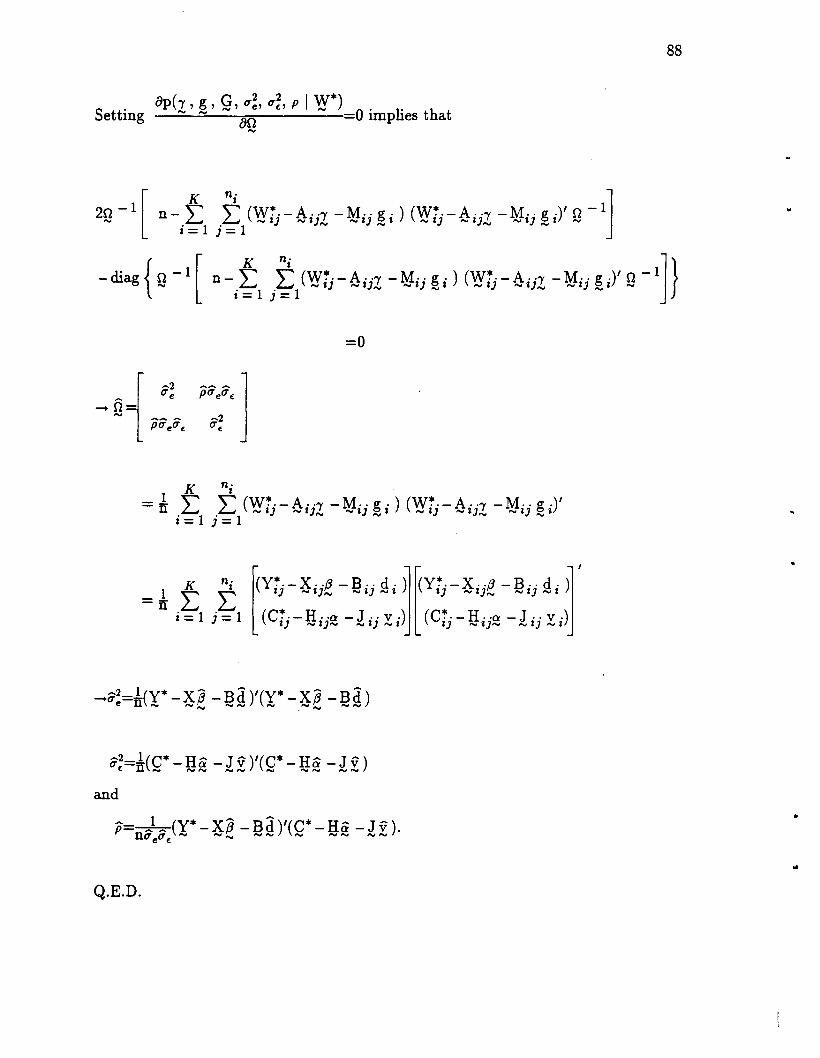
88
8p('Y, g, G, O"~, O"~, p I W*)Setting ........"" ao .... 0 implies that
....
[
K ni ]20 - 1 n - '"' '"' (W'!. - A ..'Y - M· . g . ) (W'!. - A "'Y - M· . g .)/ 0 - 1.... .L..J
1.L..J
1.... J} .... J}.... .... J} .... J .... J} .... J}.... .... J} .... J ....
J = } =
K ~ ]}n - '"' '"' (W'!. - A ..'Y - M· . g . ) (W'!. - A .''Y - M· . g .)/ 0 - 1L..J L..J .... J} .... J}.... .... J} .... J .... J} .... J}.... .... J} .... J ....i=1 i=1
=0
K ni= -n1 '"' '"' (W'!.-A ..'Y -M·· g.) (W'!.-A ..'Y -M·· g .)/.L..J .L..J .... J} .... J}.... .... J} .... J .... J} .... J}.... .... J} .... J
J=1 }=1
K ni
=ft L Li=1 i=1 t
y '! . - X ..{3 - B .. d . jty '! . - X ..{3 - B .. d . j/J} .... J}.... .... J} .... J J} .... J}.... .... J} .... J
(C'! .- H ··a - J .. v.) (C'!' . - H ··a - J .. v .)J} .... J}.... .... J} .... J J} .... J}.... .... J} .... J
_(j2e=-n1(y*-XP -Bd)/(Y*-XP -Bd)f!OtJ fiOtJ""J ""J""J f"V ,f!OtJ"'V NN
and
Q.E.D.
•
..
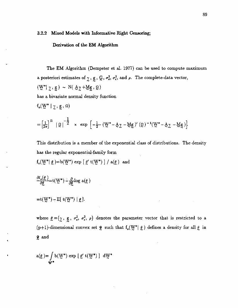
89
3.2.2 Mixed Models with Informative Right Censoring;
Derivation of the EM Algorithm
The EM Algorithm (Dempster et al. 1977) can be used to compute maximum
a posteriori estimates of 'Y , g , G, O'~, 0';, and p. The complete-data vector,'"" '"" '""
(\,Y*I 2: ' ~) '" N( ~ 2: +¥~ , 9)
has a bivariate normal density function
1=[2~Jn 191-2 x exp [-~(\,Y*-~2:-¥~)'(9)-1(\'y*_~Z -¥2)).
This distribution is a member of the exponential class of distributions. The density
has the regular exponential-family form
fo(\'y*/ fl )=b(\'y*) exp [ !l' t(\'y*) ] / a(fl) and
=t(\'y*) -:- E[ t(\'y*) I fl].
where fl ={2:' 2' O'~, 0';, p} denotes the parameter vector that is restricted to a
(p+1)-dimensional convex set ! such that fo(\'y* I fl) defines a density for all fl in
~ and'""
a(fl)= Jb(\'y*) exp [ !l' t(\'y*)] d\'y*W'*

90
where w* is the sample space of Vj*.
For a right censored sample (Vj, f) the function
Q(~, f )=E[lo(& IVj*)+log 1r(g 1 I 91) I Vj, f, f]-=E[fJt(Vj*)-loga(~) I Vj,f,f]+logb(Vj*)+log1l"(~11 91)
=E[ fJt(Vj*) I Vj, f, f] -log a(~)+log b(Vj*)+log 1l"(~ 1 I 91)·
For a concave function Po' Q is maximized with respect to ~ when
0= oQ(~, f) E[ t(W*) I W 6 0] _0 log a(fi) + -L log 1r(g I G )o~ - - ,- , - Ofl of I _ 1 - 1
or E[ t(Vj*) I Vj, f, f]=E[ t(Vj*) I~] - oil log 1l"(~ 1 I 91)·
The corresponding E and M steps are:
E-step: Compute t(r)(Vj*)=E[ t(Vj*) I Vj, f , fer -1)]
M-step: Obtain f(r)as the solution to
E[ t(W*) I oCr)] --O-log 1r(g (r) I G(r))=t(r)(w*).- - 00 (r) - - --
(3.2.3)
With bivariate right censoring, there are three cases to be considered:
(1) 6lij=c2ij=1, i.e., both Yij and Cij are known,
(2) 61ij=1 and 62ij=0 which implies that Cij>Yij=Y ij
and (3) 61ij=0 and 62ij=1 which implies that Yij>Cij=Cij .
It is assumed that at least one of the Yij or Cij is observed. If both are missing
(i.e., 6Iij=62ij=0), this observation is assumed to be ignorably missing.
..

In the expectati?n step,
E[ t(W:t:.) I W· ·=w·· 0·· (J]=IJ IJ IJ' -IJ' -
0lil2ijE[ t(Wij)l Wij=wij' 0lij=l, 02ij=1, f]
+(1- 0li)02ijE[ t(Wi'j) I Wij=wij' 0lij=O, 02ij=1, f]
+c5li/1- 02ij)E[ t(Wij) , Wij=wij' 0lij=l, 02ij=0, f]
=°1..°2..E[ t(W:t:.), W:t: ·=w··, (J ]IJ IJ IJ IJ IJ-
+(1-°1..)°2 E[ t(W:t:.) I y:t:.>y .. C:t:·=y·· (J]IJ ij IJ IJ IJ' IJ IJ' -
+°1..(1 - 02 )E[ t(W:t:.) I y:t: .=y.. C:t: .>y.. (J]IJ ij IJ IJ IJ' IJ IJ' -
=c51ijc52ijt(Wij)
+(1-°1..)°2 E[ t(W:t:.) I y:t:.>y .. C:t:·=y·· (J]IJ ij IJ IJ IJ' IJ IJ' -
+c51ij(1- 02ij)E[ t(Wi'j) I Yij=Yij, Cij>Yij' f]
with corresponding density functions
91
fo(Y*=y*, Y=y, °1=0, °2=1)
fo( Y=y, °1=0, 02=1)
00
gC*(y) / fo(Y*' C*=y) dY*y
fo(Y*=y*, C*=y)00
/ fo(Y*, C*) dY*y
00
/ fo(Y*' C*=y) dY*y
fo(Y*' C*=y)
1- ~(zY*1c*)

where Zy. Ic·, ij
and
y .. -[X ..{3 +B·· d +/'Y·[y .. - (H"Q +J .. v.)]]IJ "" IJ"" "" IJ "" 1 (fc. IJ "" IJ"" "" IJ "" 1
1(fy.(1- p2)2
92
fo(C*=c*, Y=y, 61=1, 62=0)fo( Y=y, 61=1, 62=0)
60
fy*(y) Jgo(C·1 y*=y) dC*y
fo(Y*=y, C*=c*)00Jfo(Y·, C*) de*y
00Jgo(C·' y*=y) dC*y
go(C·' Y*=y)1- ~(zc.1 y.)
where zc· IY·, ij
Therefore
[(fc· ]Y· .- H··Q +J .. v +n-=-[y .. - (X ..{3 +B .. d .)
IJ ""IJ"" ""IJ ""I r u y • IJ ""'J"" ""IJ ""I1
(fc.(1- p2)2
00
1 - ~(Zy: Ic', ;;) !.t(Wij ) fo(Yij I CirY;j' f ) dYij'J,
..

and
E[ t(Wij) IYij=Yijl Cij>Yijl f]
00
1- c)(ZC: I y* 1 ij) y/.t(Wij ) go(Cij IYij=Yijl f) dCij'lJ
93

94
3.2.3 Mixed Models with Informative Right Censoring; EM Computations
EM Computations are summarized in this section. In the E step, the
conditional expected values of the 'complete-data' sufficient statistic are computed
from the observed data and current estimates of the parameters, while in the M
step, new estimates of the unknown parameters are computed using the conditional
expected values of the 'complete-data' sufficient statistics in the maximum a
posteriori estimating equations.
E s.t!m:
In the r-th iteration, the estimation step computes the conditional expected
values of the complete-data sufficient statistics given the observed data Vj and the
estimated values of the parameters from the (r -l)-st iteration. Not all of the Vj*
are observed so the E step will estimate the complete-data sufficient statistics that
involve W*.'"
A set of complete-data sufficient statistics for this problem is
..
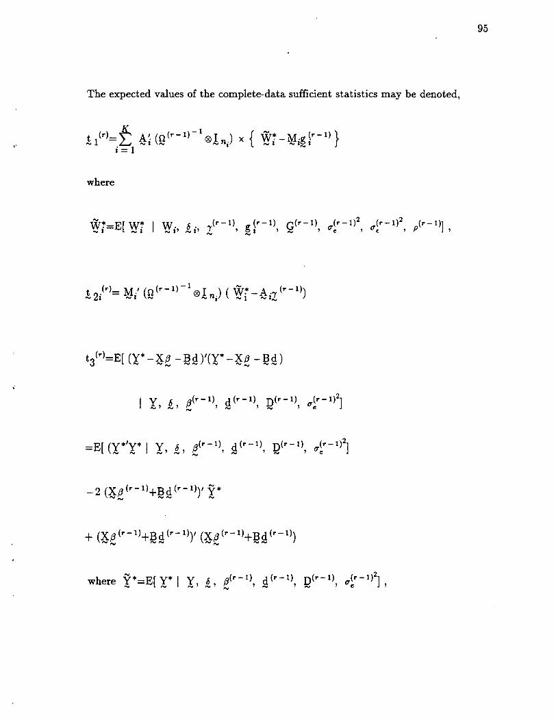
The expected values of the complete-data sufficient statistics may be denoted,
where
95
t (r)=E[ (Y*-X[3 -Bd)'(Y*-X[3 -Bd)3 ,...., "'-,...., ,....,,...., ,...., ,....,,...., ,....,,....,
I Y C [3(r-l), d(r-l) n(r-l) (T(r-l)2]""",,' £' ,...., ,...., ',...., 'e
=E[ (y*'y* I Y 6 [3(r-l), d (r-l) n(r-l) (T(r-1)2],...., N "",',....,' flOW ,...., ',...., 'e
(r -1)]P ,

96
I Y c (r - 1) (r - 1) y(r - 1) (r - 1)2]"", z' 2 ,~ '"" ,u(
'"
where Q*=E[ (C* I Y 0 a(r-l) v(r-l) y(r-l)._ .-- ""J' f"tJ' ""'J 'f"tJ 'f'V ,
and
..I W 0 (r-l) g(r-l) a(r-l)
"" i' "" i' Z '"" ~ '"" ,
(r _1)2 p(r -1)](f ( ,
When 0lij=O and 02ij=1 expectations involving the i-th element of the complete
data sufficient statistics can be computed as:

00 f (y* I C* - 0(,.-1»)=1 Y!· 0 ij ij-Yij' - dY!·J) l-<I>(Z(,..-I)•..) J)
Yij Y IC , J)
where
97
(,. -1)ZY·IC·, ij
and
[
(,.-1) ]y .. _ X ...a(,.-I)+B ..d(,.-I)+ (,.-I)O"e [y .. _(H ..C/,.-I)+J ..V(,.-I))]
J) _ J)_ - J)_J P (,. -1) J) - Z)_ _ Z)_ ZO"e
00 f(Y*IC*- 0(,.-1»)= 1Y!~ 0 ij ij-Yij' - dY!·
Z) l-<I>( (,.-1) ..) Z)Yij Zy. IC·, J)

98
(r -I)+ (r-1}O'e (y .. _H ..a(r-1}_J "V(r-1})]p (r-1) J) _J)_ _J)_J
O'~
A.( (r-1) )'I' zY* Ic*, ij
x 1 &( (r - I) ) .-'f!' zY*lc*, ij
Similarly, when 61ij=1 and 62ij=O expectations involving the i-th element of the
complete-data sufficient statistics can be computed as:
00 (C*IY*- O(r-1})=j C'!'. go ij ij-Yij' - dC'!'.
J) 1-;"'( (r-1) ..) J)Yij 'f!' Zc* IY·, J)
A.( (r-1) )'I' ZC* IY·, ij
1 ~((r-1) )- ZC·'Y·, ij
where
(r -I)ZC·IY·, ij
and
E[Ci] IYij=Yij, Cij>Yij, !(r -I)]
,.

99
=7Yij
(C* I Y* -Y O(r -1»)C'~~ go ij ij- ij' '" dC'!'.
ZJ 1 ((r-l») ZJ-~ zc* IY*, ij
.'
[ H (r-l) J (r-l)x y. + "0' + ..vZJ .... zJ.... .... zJ.... Z
(r -1)+ (r-l)U( (y .. _x ..j3(r-l)_B ..d(r-l»)]
p (r-l) zJ .... zJ.... ....zJ....zUe
A.( (r-l) )'I' ZC*IY*, ij
x 1 A'..( (r - 1) ) •- 'f! ZC* IY*, ij
.'
M~:
The r-th iteration of the M step obtains 'Y (r) g (r) G (r) u(r)2 u(r)2 and p(r) as~ '1'OtoI ' f"W , e , (: ,
the solution to equation 3.2.3. Initial values of maximum a posteriori estimates are
obtained using unweighted regression and by treating censored data as if they were
uncensored. Convenient initial estimates are:

100
mand if 9= L Us § s then
s=l
In the r-th iteration maximum a posteriori estimates which maximize the posterior
distribution function using the expected values of the complete-data sufficient
statistics obtained from the previous iteration of the E step are computed:
[ K ]-1-y(r)= ~A./(O(r-I)-lI8lI )A. t (r)"'" LJ "'" 1 "'" "'" nj "'" 1 "'" 1 ,
i = 1
g (r)=[ M.' (O(r-l)-lI8lI ) M+G(r-l)-l].-l t (r)~ I #'IV Z ~ N ni ""J I "'tJ N 2i '
K IG(r)=.l.. ~ g (r)g (r)"'" K.LJ "'" 1 "'" 1 ,
1=1
(r)2_1 t (r)u£ -IT 4 '
..

1 t (r)(r-l) (r-l) 5 '
nO'e O'~
mand if Q=I: T S § s then
s=1
101

102
IV. EXERCISE TOLERANCE TESTS OF PATIENTS WITHCHRONIC STABLE ANGINA
4.1 Introduction
Calcium channel blocking drugs have been found to be useful in the treatment
of patients with chronic stable angina. Nisoldipine, a dihydropyridine slow channel
calcium blocker is a potent coronary vasodilator and could be beneficial for patients
with angina. Lam et al. (1985) conducted a placebo-controlled, double-blind
crossover, dose-ranging study to assess the short-term efficacy of nisoldipine as an
antianginal drug in humans. Maximal treadmill exercise tests at 1, 3 and 8 hours
after ingestion of a single dose of a placebo or a 5, 10, or 20 mg. oral dose of
nisoldipine were used to assess the duration of its effects and the effective oral dose.
The efficacy of nisoldipine was assessed in terms of time to onset of angina
(denoted by Y*), the primary response of interest, and other response variables.
Because the greatest effects occurred 3 hours after oral ingestion, we shall examine
the 3-hour data.
The dataset described in Lam et al. (1985), reproduced in Appendix A, was
used to obtain parameter estimates assuming that no censoring occurred. Those
parameter estimates were used as parameter values in a program that generated
artificial data for 80 subjects. (The details are described in Section 4.3.) Fixed and
informative right censoring were induced artificially and resulting parameter
estimates are compared to those obtained without censoring in Section 4.4. Fixed
censoring occurs when time to onset of angina exceeds a predetermined value.
Informative right-censoring occurs when time to onset of angina exceeds maximal
..

103
exercise time (denoted by C*), the censoring variable. In this situation, patients
become exhausted and have to stop running on the treadmill before they get
angma. However because peak exercise duration time and time to onset of angina
are highly correlated, it is plausible that individuals are censored when they were
at unusually high risk of failure.
104
4.2 Description of the Experiment and Data
The study population consisted of 12 male or female patients with a mean age
of 58 years (range 46 to 66) who had a history of angina pectoris which had been
stable for at least three months. Prior to acceptance into the study, exercise
induced angina occurred during upright treadmill exercise tests in all of these
patients, with specified associated ECG changes. Three patients had a previous
myocardial infarction and one patient had prior coronary bypass surgery. Patients
were excluded from the study if they had a history of predominant rest angina or
ST segment elevation during an episode of chest pain, severe hypertension, valvular
heart disease, congestive heart failure, intraventricular conduction disturbances or
severe ventricular arrhythmias on the electrocardiogram at rest.
Patients were randomized to one of four treatment sequences and received a
different dose each visit. Prior to entering the study, each patient had had at least
two exercise tests and were familiar with the test environment. All cardiovascular
medications were stopped at least 48 hours before the study with the exception of
nitroglycerin, which was stopped at least eight hours before the exercise test.
Patients also refrained from smoking and drinking coffee o~ tea at least eight hours
before the exercise test. A single oral dose consisting of four tablets was given at
8:00 AM. The placebo dose consisted of four placebo tablets, the 5 mg. dose
consisted of one 5 mg. tablet of nisoldipine and 3 placebo tablets, the 10 mg. dose
consisted of two 5 mg. tablets of nisoldipine and two placebo tablets, and the 20
mg. dose consisted of four 5 mg. tablets of nisoldipine. Modified Naughton
treadmill exercise tests were performed at 9:00 AM, 11:00 AM and 4:00 PM.
Exercise tests were terminated due to severe angina or extreme fatigue. The series
of tests involved four study days per patient and were completed within 2 weeks for
each patient. There was a 48 to 72 hour washout period after each visit. Previous
•

105
data had indicated that a 48-hour washout period was sufficient to eliminate
carryover effects.

106
4.3 Computational Issues
Recall that the mixed model for Wi is given by
where
Wi is a 2ni x 1 vector of failure and censoring values which mayor may not
be observed,
..
[
X.A.= -I-I 0- ~. ] is a 2ni x 2p known constant matrix of rank 2r $ 2p,
-I
x~ ;] is a 2p x 1 vector of unknown constant 'fixed' population parameters,
[ B0 ]M.= -I -
-I 0 J.- _I
g.= [2~ is a 2q x_I V.
-I
is a 2ni x 2q known matrix corresponding to the
random effects,
1 vector of unobservable individual parameters,
~ i=[~ il is a 2ni x 1 vector of unobservable random errors,!d
~ i "'" N(Q, g) independent of ~ i "'" N(Q, g ~! n),
•

107
9 is a positive-definite symmetric 2q x 2q covariance matrix
of random effects, g i' andN
consists of the unknown within-subject
variance components.
The formulae given in Sections 3.1.3 and 3.2.3 were used to obtain parameter
estimates, with the exception of initial starting values. These were estimated
assuming noninformative censoring and using the EM algorithm to compute
maximum likelihood estimates of {3, D, and .O'~.. The same initial estimates of {3,N N N
:Q, and O'~ were used in the informative censoring program. It was assumed that
~ (O)=e (0), y(O)=:Q (0), 0'~0)2 =0'~0)2, cov(y(O), 12(0))=0.5, and p=0.5. These estimates
were then used to obtain initial estimates of the random effects.
Convergence was assumed to have occurred if the maximum relative change
(over all estimators) in one iteration was less than 0.001 for all of the structural
parameters. Using the values of the parameters at convergence, the observed log
posterior distribution functions assuming fixed or noninformative censoring and
informative censoring were:
p(e, 2, 12, O'~I y, §. )
and
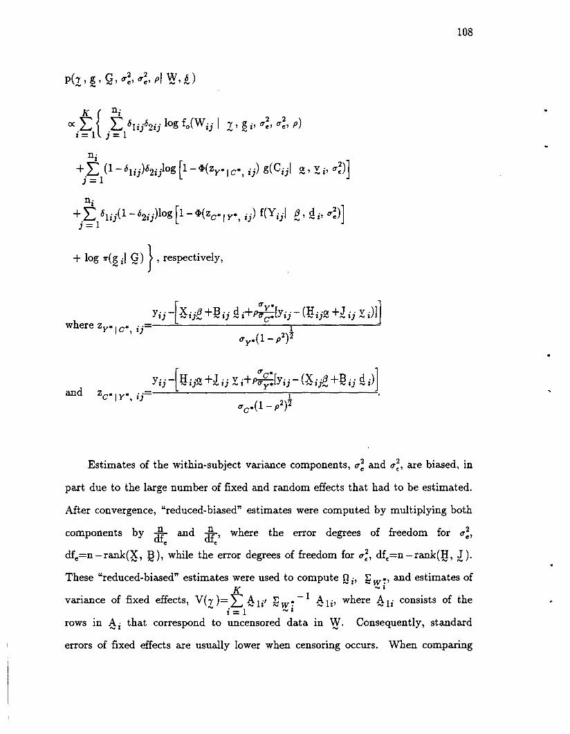
108
ni
+j~/lij(1-c52ij)log[1-41(ZO·IY.'ij) f(Yijl £' Qi' O'~)]
+ log r(~;1 m},respectively,
..
where Zy. 10·, ijY·· -[X ..,8 +B .. d+pO'Y·[y .. - (H ..cr +J .. v.)]]
J) - J)_ - J) - J 0'0. J) - J)_ - J) - J
1
O'y.(l- p2ri..
and ZO·I Y·, ij[
0'0· ]Y··- H··cr+J·· v +~[y .. _(X ..,8+B .. d.)J) _ J)_ _ J) _ J 0'y. J) - J)_ - J) - J
1
0'0.(1 - p2)2
Estimates of the within-subject variance components, O'~ and O'~, are biased, in
part due to the large number of fixed and random effects that had to be estimated.
After convergence, "reduced-biased" estimates were computed by multiplying both
components by dt and dt' where the error degrees of freedom for O'~,e (
dfe=n - rank(~, ~), while the error degrees of freedom for O'~, df(=n - rank(IJ, ~).
These "reduced-biased" estimates were used to compute Qi' ~ w,!" and estimates ofK _J
variance of fixed effects, V(Z)= L ~ Ii' ~ w'!' -1 ~ li' where ~ Ii consists of thei = 1 - J
rows in ~ i that correspond to uncensored data in V:!. Consequently, standard
errors of fixed effects are usually lower when censoring occurs. When comparing

109
approximate standard errors of fixed effects with and without censored data, it may
be preferable to use all the rows of ~i instead of using ~ Ii'
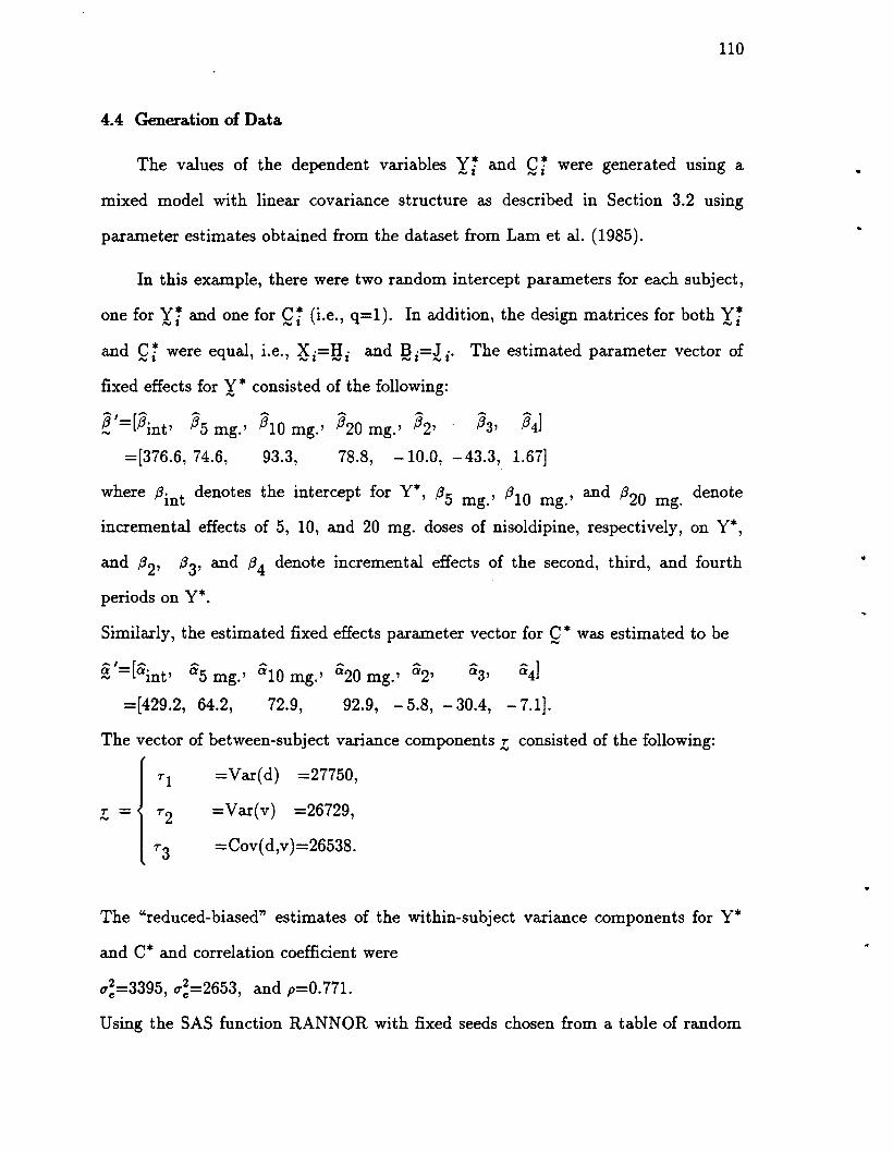
110
4.4 Generation of Data
The values of the dependent variables y; and Q; were generated usmg a
mixed model with linear covariance structure as described in Section 3.2 using
parameter estimates obtained from the dataset from Lam et al. (1985).
In this example, there were two random intercept parameters for each subject,
one for y; and one for Q; (i.e., q=l). In addition, the design matrices for both y;and Q; were equal, i.e., ~i=tli and :§i=li' The estimated parameter vector of
fixed effects for y * consisted of the following:
e'=[,8int' ,85 mg.' ,810 mg.' ,820 mg.' ,82' ,83' ,84]
=[376.6, 74.6, 93.3, 78.8, -10.0, - 43.3, 1.67]
where {3. t denotes the intercept for Y*, {35 ,{310 g' and {320 denotem mg. m . mg.
incremental effects of 5, 10, and 20 mg. doses of nisoldipine, respectively, on Y*,
and {32' {33' and (34 denote incremental effects of the second, third, and fourth
periods on Y*.
Similarly, the estimated fixed effects parameter vector for Q* was estimated to be
€'=[aint' a5 mg.' alO mg.' a20 mg.' a2' a3' a4]
=[429.2, 64.2, 72.9, 92.9, -5.8, -30.4, -7.1].
The vector of between-subject variance components z; consisted of the following:
Tl =Var(d) =27750,
T - T2 =Var(v) =26729,"'"
T3 =Cov(d,v)=26538.
The "reduced-biased" estimates of the within-subject variance components for Y*
and C* and correlation coefficient were
0-;=3395, 0-;=2653, and p=0.771.
Using the SAS function RANNOR with fixed seeds chosen from a table of random
..

111
digits, ~ i and ~ i were generated for eaeh subject. Because ~ i - NID(Q, g), data
can be generated by setting
1 1
~i=g2~9i and Wij=~ijZ+¥ij~i+Q2~ij'
1 1
where ~ gi and ~ ij are 2 x 1 NID(O, 1) random variables and ~? and Q2 are the
Cholesky square roots of 9 and Q. Data were generated for 80 subjects with up to
four visits per subject (Appendix B). One of four treatment sequences was
randomly assigned to each subject with equal probability using the SAS function
RANUNI. To ensure that some data were missing at random, .observations were
deleted with a 15% probability. This would reflect a situation in which, on
average, subjects failed to show up for their scheduled appointments 15% of the
time.
This data were analyzed with and without censormg. Right censormg was
induced by censoring either the time to onset of angina or the maximal exercise
time, whichever was greater if they exceeded the seventy-fifth percentiles." In this
dataset, the seventy-fifth percentiles were 540 seconds for time to onset of angina
and 556 seconds for MET. Ten percent (28) of the 273 observed angina times and
19% (53) of the 273 realized values of maximal exercise time were censored. Note
that computations that assume censoring is informative will make adjustments for
30% of the observations that have either censored angina or maximal exercise
times. If censoring is assumed to be fixed, maximal exercise time is irrelevant and
adjustments only need to be made for 10% of the censored angina times.
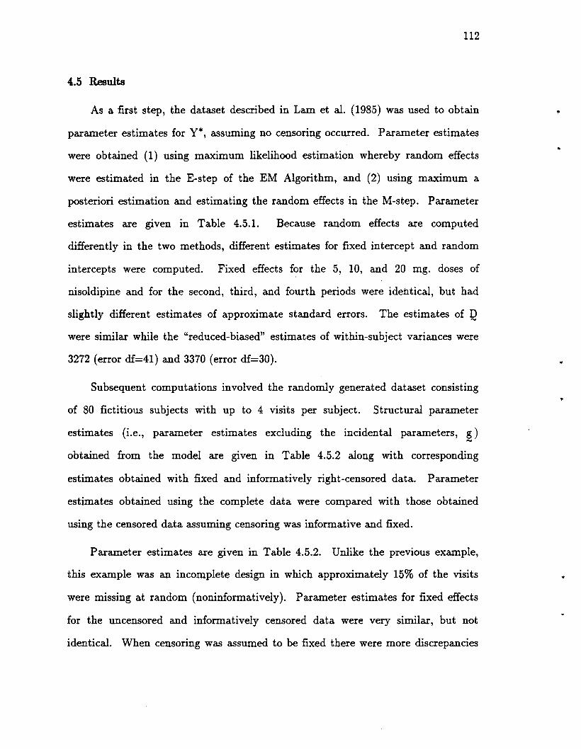
112
4.5 Results
As a first step, the dataset described in Lam et ale (1985) was used to obtain
parameter estimates for Y*, assuming no censoring occurred. Parameter estimates
were obtained (1) using maximum likelihood estimation whereby random effects
were estimated in the E-step of the EM Algorithm, and (2) using maximum a
posteriori estimation and estimating the random effects in the M-step. Parameter
estimates are given in Table 4.5.1. Because random effects are computed
differently in the two methods, different estimates for fixed intercept and random
intercepts were computed. Fixed effects for the 5, 10, and 20 mg. doses of
nisoldipine and for the second, third, and fourth periods were identical, but had
slightly different estimates of approximate standard errors. The estimates of Q
were similar while the "reduced-biased" estimates of within-subject variances were
3272 (error df-41) and 3370 (error df=30).
Subsequent computations involved the randomly generated dataset consisting
of 80 fictitious subjects with up to 4 visits per subject. Structural parameter
estimates (i.e., parameter estimates excluding the incidental parameters, g)....
obtained from the model are gIven in Table 4.5.2 along with corresponding
estimates obtained with fixed and informatively right-censored data. Parameter
estimates obtained using the complete data were compared with those obtained
using the censored data assuming censoring was informative and fixed.
Parameter estimates are given in Table 4.5.2. Unlike the previous example,
this example was an incomplete design in which approximately 15% of the visits
were missing at random (noninformatively). Parameter estimates for fixed effects
for the uncensored and informatively censored data were very similar, but not
identical. When censoring was assumed to be fixed there were more discrepancies
,.
..

..
113
between parameter estimates obtained for uncensored data and censored data.
This is not surprising because the correlation between Y* and C* was ignored.
The estimated variance components that were computed assuming fixed
censoring were somewhat smaller than those that were computed using uncensored
or informatively censored data. This resulted in somewhat larger estimates of
approximate asymptotic standard errors for fixed effects. Approximate asymptotic
standard errors of fixed effects parameters obtained using informatively censored
data were smaller than those obtained using the uncensored data.
Results in Tables 4.5.1 and 4.5.2 indicate that time to onset of angina and
peak exercise time were both prolonged by each dose of nisoldipine. In these data,
the 10 mg. dose was optimal for prolonging time to onset of angina while the 20
mg. dose was optimal for prolonging maximal exercise time. Period effects were
minimal in the original 12-patient dataset but appeared to be present in the larger
SO-patient dataset, most likely due in part to the larger sample size and
corresponding smaller standard errors.
Maximum a posteriori informative censonng estimates and maxImum
likelihood estimates and approximate asymptotic standard errors from Tables 4.5.2
and 4.5.3 are plotted in Figure 4.5.1, along with the population estimates (i.e, the
original parameter values, denoted by *, that were used to generate the larger
sample). The predicted response, Time to Angina (seconds), is plotted against
estimates of fixed effects parameters for incremental effects of the 5, 10, and 20 mg.
doses of nisoldipine and incremental effects of the second, third, and fourth test
days. Approximate 95% confidence intervals for incremental effects of the 5, 10,
and 20 mg. doses do not include zero. The largest incremental effect corresponded
to the 10 mg. dose where the predicted increase in time to onset of angina was 95.3

114
seconds using all the data, 83.5 seconds after deleting censored observations, and
91.0 seconds using the casewise deletion method. The overlap of the approximate
confidence intervals suggest that the treatment effects are not significantly different
from one another but do seem to be significantly different from the placebo.
Incremental effects due to the second and fourth test days do not appear to be
statistically significant at the a=0.05 level. However, patients appeared to perform
poorly on the third test day with predicted decreases in time to angina of about 60
seconds.
Maximum likelihood estimates in Table 4.5.3 were computed usmg mixed
model techniques for complete data after (1) deleting 10% of the 273 observations
with censored values of time to onset of angina and (2) "Casewise Deletion", where
patients were excluded from the analysis if any of their angina times were either
censored or missing. Casewise deletion resulted in the greatest loss of information
46 of the 80 patients (58%) were excluded from the analysis. As a result, one
would expect these confidence intervals to be the most inaccurate and to have the
largest standard errors.
The discrepancies between the confidence intervals appear to be particularly
evident for the 20 mg. dose. Using the casewise deletion method, the predicted
increase in time to onset of angina was only 31.2 seconds compared to 63.0 seconds
using the informatively censored angina times and 53.3 seconds using the mixed
model approach assuming that censored angina times were missing at random.
Note also that the confidence intervals for the casewise deletion method are wider
and would lead one to believe that the incremental effect of the 20 mg. was the
least effective dose.
...
..
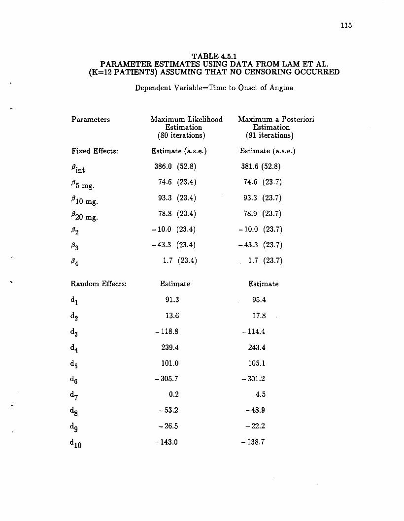
TABLE 4.5.1PARAMETER ESTIMATES USING DATA FROM LAM ET AL.
(K=12 PATIENTS) ASSUMING THAT NO CENSORING OCCURRED
Dependent Variable=Time to Onset of Angina
Parameters Maximum Likelihood Maximum a PosterioriEstimation Estimation
(80 iterations) (91 iterations)
Fixed Effects: Estimate (a.s.e.) Estimate (a.s.e.)
.8int 386.0 (52.8) 381.6 (52.8)
.85 mg. 74.6 (23.4) 74.6 (23.7)
.810 mg. 93.3 (23.4) 93.3 (23.7)
.820 mg. 78.8 (23.4) 78.9 (23.7)
.82 -10.0 (23.4) -10.0 (23.7)
.83 -43.3 (23.4) -43.3 (23.7)
.84 1.7 (23.4) 1.7 (23.7)
Random Effects: Estimate Estimate
d1 91.3 95.4
d2 13.6 17.8
d3 -118.8 -114.4
d4 239.4 243.4
dS 101.0 105.1
d6 -305.7 -301.2
d7 0.2 4.5
d8 -53.2 -48.9
d9 -26.5 -22.2
dlO -143.0 -138.7
115

Parameters Maximum LikelihoodEstimation
(80 iterations)
43.9
335.4
Maximum a PosterioriEstimation
(91 iterations)
48.1
339.2
116
Variance Components:
D 27754
3272
27545
3370
a.s.e. = approximate asymptotic standard error
..

117
TABLE 4.5.2MAXIMUM A POSTERIORI PARAMETER ESTIMATES
USING SIMULATED DATASET (K=80 PATIENTS)
Dependent Variables=Time to Onset of Angina,Maximal Exercise Time.
'"
Parameters Complete Data Informative Censoring Fixed Censoring·(83 iterations) (80 iterations) (52 iterations)
Fixed Effects: Estimate (a.s.e.) Estimate (a.s.e.) Estimate (a.s.e.)
.8int 382.2 (17.3) 383.5 (10.0) 386.8 (15.0)
.85 mg. 60.5 (11.5) 61.8 (10.5) 57.2 (12.0)
.810 mg. 94.3 (11.1) 95.3 (10.4) 96.5 (12.2)
.820 mg. 62.5 (10.7) 63.0 (9.3) 58.1 (11.3)
.82 -13.8 (11.2) -15.2 (10.0) -16.7 (12.1)
.83 -57.9 (11.3) -59.0 (10.2) -59.4 (12.1)
.84 -4.6 (10.9) -4.6 (9.5) -9.0 (11.6)
Qint 438.8 (15.6) 438.9 (8.9)'f
Q5 mg. 53.4 (9.8) 4;8.0 (9.2)
QlO mg. 59.2 (9.4) 55.9 (8.7)
Q20 mg. 74.7 (9.1) 70.5 (8.6)
Q2 -13.6 (9.5) -14.7 (8.7)
Q3 -38.6 (9.6) -38.4 (8.9)
Q4 -23.4 (9.2) -24.7 (8.3)
...
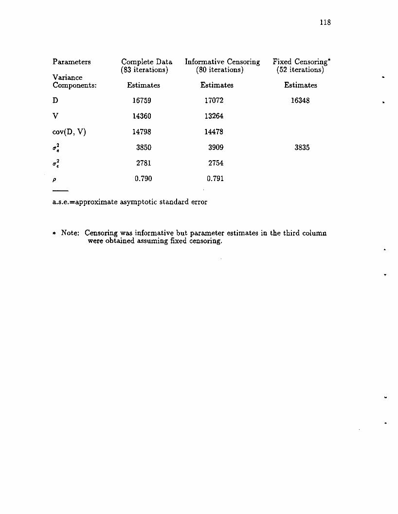
118
Parameters Complete Data Informative Censoring Fixed Censoring*(83 iterations) (80 iterations) (52 iterations)
VarianceComponents: Estimates Estimates Estimates
D 16759 17072 16348 ..
V 14360 13264
cov(D, V) 14798 14478
rr2 3850 3909 3835e
rr2 2781 2754(
p 0.790 0.791
a.s.e.=approximate asymptotic standard error
* Note: Censoring was informative but parameter estimates in the third columnwere obtained assuming fixed censoring.
..

TABLE 4.5.3MAXIMUM LIKELmOOD ESTIMATES
USING SIMULATED DATASET
Dependent Variable=Time to Onset of Angina
.:
Parameters Censored Observations Casewise DeletionDeleted (K=78) (K=34)(38 iterations) (91 iterations)
Fixed Effects: Estimate (a.s.e.) Estimate (a.s.e.)
.8int 383.2 (17.2) 368.0 (26.8)
.85 mg. 53.8 (11.9) 59.6 (16.5)
.810 mg. 83.5 (12.1) 91.0 (16.5)
.820 mg. 53.3 (11.1) 31.2 (15.0)
.82 -15.8 (11.9) -16.1 (16.5)
.83 -57.7 (12.0) -62.4 (16.5)
.84 -9.7 (11.4) -12.0 (15.0)
Variance Components:
119
D
0-2e
15549
3650
17551
3540
a.s.e. = approximate asymptotic standard error
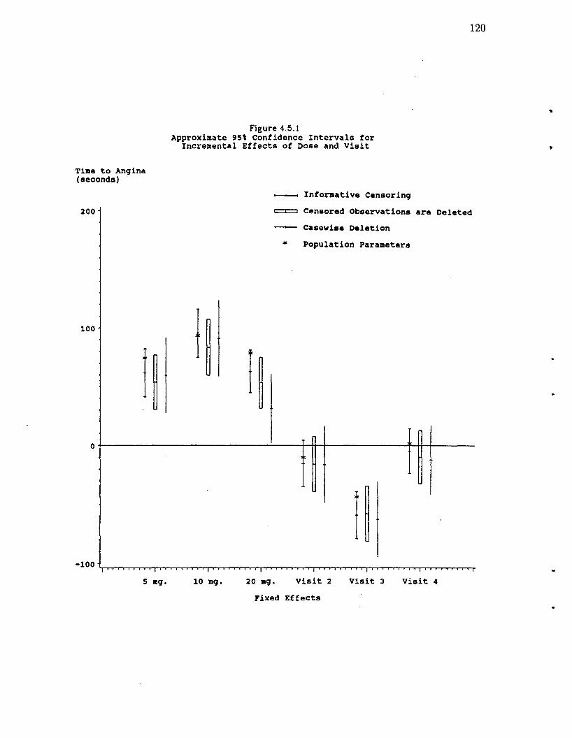
Time to Angina(seconds)
Figure 4.5.1Approximate 9St Confidence Intervals for
Incremental Effects of Dose and Visit
~ Informative Censoring
120
200
100
o
-100
~ Censored Observations are Deleted
- casewise Deletion
* PopUlation Parameters
!~f ~
I~
nI I
5 mg. 10 mg. 20 mg. Visit 2 Visit 3 Visit 4
Fixed Effects

121
4.6 Summary
Results from a demonstration of this method using the treadmill exercise data
from the cross-over study by Lam et al. (1985) and the simulated dataset generated
using this data were summarized in this chapter. In each example, the algorithm
was monotonic: the logarithm of the posterior distribution function increased
monotonically until the parameter estimates converged within the specified
tolerance. Estimates of fixed effects and variance components obtained after
censoring approximately 10 to 30% of the data were reasonably close to the original
complete-data estimates and were well within two standard errors of one another.
Parameter estimates for incremental effects of dose were somewhat higher
when right-censoring was taken into account than when censored observations were
deleted. This would always be the case if censored data had been analyzed as if
they were uncensored. The least accurate method was casewise deletion, where
58% of the patients were excluded from the analysis.

122
v. SUMMARY AND RECOMMENDATIONS FOR FUTURE RESEARCH
5.1 Summary
The purpose of this work was to simplify existing computational approaches
used to estimate parameters in general linear mixed models with fixed or
noninformative random censoring and to extend the use of these techniques to
include parameter estimation in mixed models with informative censoring. This
method is applicable to normal data from longitudinal studies where the effects of
serial correlation are negligible.
For this type of problem, the EM algorithm was preferable to gradient
methods (e.g., Newton-Raphson algorithm, Method of Scoring) because the
likelihood of the complete data for the General Linear Mixed Model has a much
simpler form than the likelihood corresponding to the General Linear Mixed Model
with censored data. The EM algorithm also does not require the inversion of large
matrices. Using the Newton-Raphson algorithm, this problem can become
overwhelming when the number of subjects is large and gets worse when there are
multiple random coefficients for each subject.
Using an extension of maximum likelihood estimation known as maximum J.k
posteriori estimation, computations involved in obtaining parameter estimates in
the M step of the EM algorithm are straightforward. Unlike the maXImum
likelihood approach, random effects are estimated in the M step instead of the E
step of the EM algorithm and do not require the computation of high-dimensional
to,
..

123
integrals.
In an example, parameter estimates obtained usmg informatively censored
data were generally quite similar to estimates obtained using complete data (i.e.,
data that were generated before being artificially censored). The extent of
agreement was usually greater if censoring was correctly assumed to be informative
than when it was assumed to be fixed. Parameter estimates obtained from the
complete data set using maximum likelihood estimation and maximum f!! posteriori
estimation were also quite similar with the exception of the within-subject variance
components.

124
5.2 Future Research
Procedures have been developed for maXImum Q posteriori estimation for a
General Linear Mixed Model for the analysis of censored normal or lognormal data,
whether or not the censoring is informative. These procedures have led to a great
reduction in computational complexities in comparison to previously available
methods for data with noninformative or fixed censoring mechanisms. Parameter
estimates obtained using informatively censored data were found to be similar to
estimates obtained using complete data. Simulation studies are needed to assess
large- and small-sample properties of the parameter estimates. Exact asymptotic
distributions of the parameter estimates under general regularity conditions also
need to be derived. This could include an evaluation of some approximate F
statistics and their small sample distributions.
"Reduced-biased" estimates of the within-subject varIance components were
proposed in this dissertation and used to compute approximate standard errors of
fixed effects. It would be useful to derive approximate asymptotic estimates of the
standard errors of random effects and variance components and to derive restricted
maximum likelihood or analogous "restricted maximum a posteriori" estimates of
variance components.
The methods developed In this dissertation are applicable to longitudinal
studies where the effects of serial correlation are negligible. These methods are
applicable when V(~ i) 1O'~. As an extension, one could attempt to model other
types of covariance structures that occur in studies of longer duration (e.g.,
irregularly-timed, inconsistently-timed longitudinal data with V(~ i) having AR(1)
covariance structures).
..
..

125
Zeger, Liang, and Albert (1988) describe how generalized estimating equations
can be used to analyze uncensored longitudinal data. They consider two
approaches: the first approach is the "subject-specific" approach where the
covariance structure is explicitly modeled, while in the second approach, the
"population-averaged" approach, the marginal expectation is the focus and the
covariance matrix is regarded as a nuisance. It may be possible to extend these
approaches so they can be used for parameter estimation in general linear mixed
models with censored data.

Appendix AAcute Effects of Nisoldipine on Chronic stable Angina
Treadmill Exercise Data (Lam et al. 1985)
Onset of CessationDose Anginal Pain of Exercise Reason for
SUbject Visit (mg) (seconds) (seconds) Discontinuation
1 1 10 540 6002 20 590 6603 0 480 510"4 5 505 530
2 1 0 395 4602 10 440 5403 5 480 5704 20 480 540
3 1 20 405 5252 5 345 3903 10 240 2854 0 260 310
4 1 5 675 6752 0 690 Fatigue3 20 660 Fatigue4 10 700 Fatigue
5 1 10 540 Fatigue2 20 585 Fatigue3 0 480 4804 5 550 570
.....t'"0)
• • .. • ,

~
Appendix AAcute Effects of Nisoldipine on Chronic stable Angina
Treadmill Exercise Data (Lam et al. 1985)
Onset of CessationDose Anginal Pain of Exercise Reason for
SUbject Visit (mg) (seconds) (seconds) Discontinuation
6 1 0 90 1202 10 110 1203 5 90 1204 20 190 210
7 1 5 450 5102 0 360 4203 20 450 5104 10 480 510
8 1 20 420 4502 5 370 4203 10 490 5304 0 240 330
9 1 0 335 3352 10 455 4803 5 420 4504 20 420 490
10 1 20 265 3602 5 290 3503 10 285 3354 0 310 370
.....~-J

Appendix AAcute Effects of Nisoldipine on Chronic stable Angina
Treadmill Exercise Data (Lam et ale 1985)
Onset of CessationDose Anginal Pain of Exercise Reason for
Subject Visit (mg) (seconds) (seconds) Discontinuation
11 1 5 540 6602 0 420 6303 20 360 6604 10 600 650
12 1 10 900 9002 20 780 7803 0 600 6604 5 840 840
~
~00
.. 4~

'1
Appendix BAcute Effects of Nisoldipine on Chronic stable Angina
Treadmill Exercise Data generated from Population Parameter Estimates
Onset of CessationDose Anginal Pain of Exercise Reason for
SUbject Visit (mg) (seconds) (seconds) Discontinuation
1 1 0 538 5562 10 572 555 Fatigue4 20 706 669 Fatigue
2 1 20 276 4022 5 383 4963 10 361 4884 0 283 355
3 1 20 345 4452 5 260 3543 10 402 4104 0 234 268
4 1 10 432 5152 20 303 4803 0 365 4734 5 433 462
5 1 20 264 3513 10 224 2734 0 167 179
6 1 20 421 4772 5 393 537
......~(0

Appendix BAcute Effects of Nisoldipine on Chronic stable Angina
Treadmill Exercise Data generated from Population Parameter Estimates
Onset of CessationDose Anginal Pain of Exercise Reason for
SUbject Visit (mg) (seconds) (seconds) Discontinuation
4 0 248 367
7 1 10 398 4203 0 288 4344 5 333 422
8 1 10 458 5272 20 547 562 Angina3 0 354 466
9 1 20 333 4982 5 294 4393 10 324 4314 0 227 342
10 1 0 437 4782 10 360 4683 5 346 430
11 1 20 350 4372 5 348 3723 10 310 3304 0 225 319
12 1 0 364 398I-'w0
• •
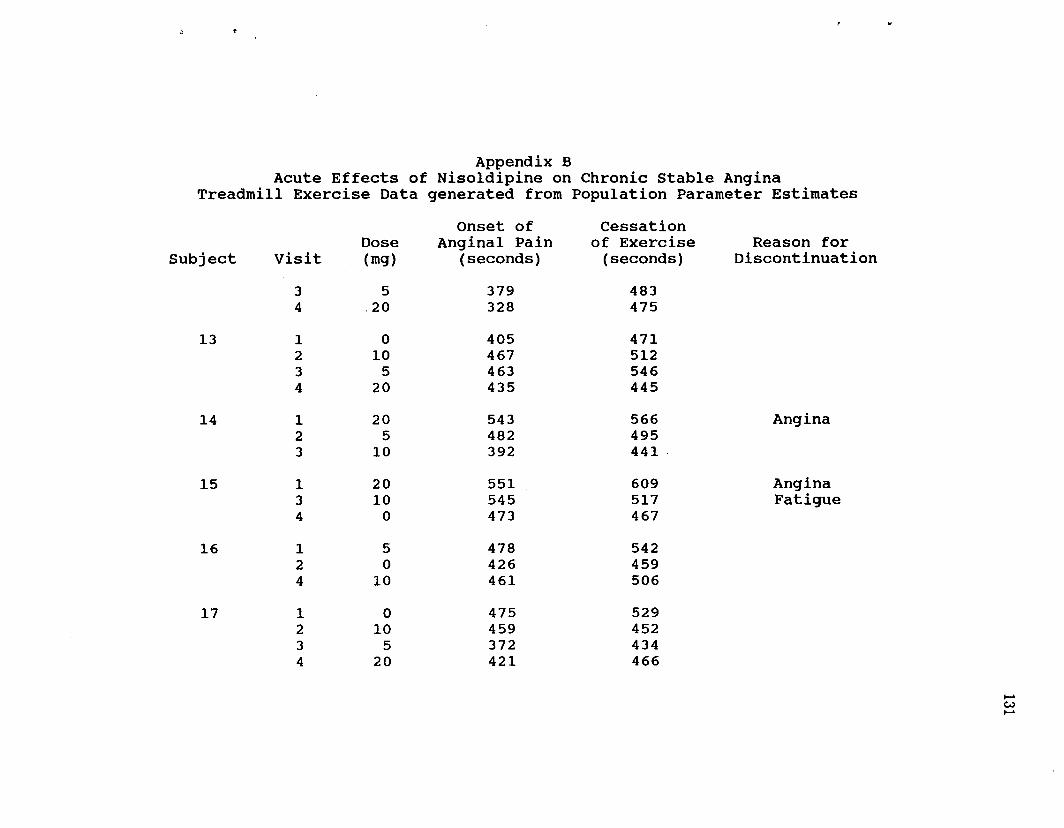
~
Appendix BAcute Effects of Nisoldipine on Chronic stable Angina
Treadmill Exercise Data generated from Population Parameter Estimates
Onset of CessationDose Anginal Pain of Exercise Reason for
SUbject Visit (mg) (seconds) (seconds) Discontinuation
3 5 379 4834 ,20 328 475
13 1 0 405 4712 10 467 5123 5 463 5464 20 435 445
14 1 20 543 566 Angina2 5 482 4953 10 392 441 '
15 1 20 551 609 Angina3 10 545 517 Fatigue4 0 473 467
16 1 5 478 5422 0 426 4594 10 461 506
17 1 0 475 5292 10 459 4523 5 372 4344 20 421 466
~
w~

Appendix BAcute Effects of Nisoldipine on Chronic stable Angina
Treadmill Exercise Data generated from Population Parameter Estimates
Onset of CessationDose Anginal Pain of Exercise Reason for
Subject Visit (mg) (seconds) (seconds) Discontinuation
18 1 20 555 549 Fatigue2 5 424 4484 0 451 413
19 1 0 375 3802 10 426 3573 5 440 3214 20 374 274
20 1 0 594 669 Angina2 10 627 632· Angina4 20 702 743 Angina
21 1 20 428 4913 10 475 4824 0 434 452
22 1 0 286 2702 10 441 3323 5 340 2964 20 442 436
23 1 0 449 4673 5 582 579 Fatigue4 20 507 445
to-'wtv
•

Appendix BAcute Effects of Nisoldipine on Chronic stable Angina
Treadmill Exercise Data generated from Population Parameter Estimates
Onset of cessationDose Anginal Pain of Exercise Reason for
Subject Visit (mg) (seconds) (seconds) Discontinuation
24 1 20 402 5002 5 470 564 Angina3 10 571 543 Fatigue4 0 367 448
25 2 0 229 3343 20 242 3544 10 332 394
26 1 10 549 509 Fatigue2 20 602 580 Fatigue3 0 376 4104 5 478 438
27 1 20 229 3362 5 95 2933 10 30 2314 0 31 150
28 1 5 152 2842 0 26 1124 10 179 179
29 1 20 491 534 -ww
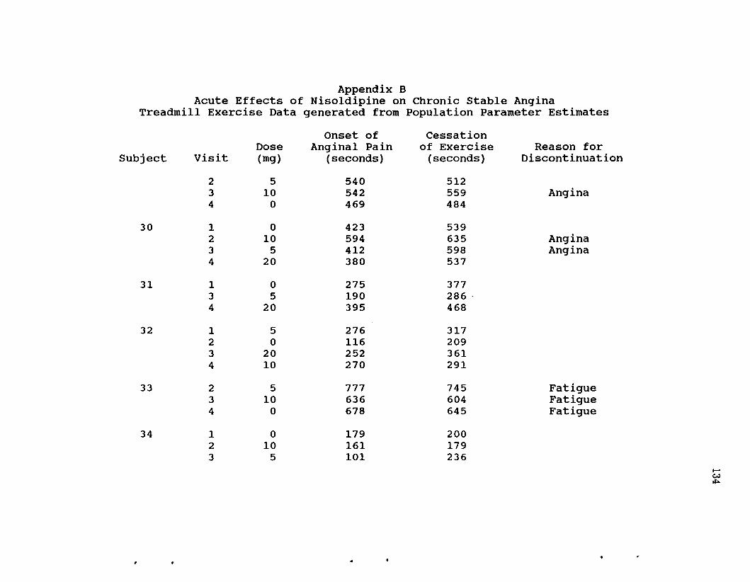
Appendix BAcute Effects of Nisoldipine on Chronic stable Angina
Treadmill Exercise Data generated from Population Parameter Estimates
Onset of CessationDose Anginal Pain of Exercise Reason for
SUbject Visit (mg) (seconds) (seconds) Discontinuation
2 5 540 5123 10 542 559 Angina4 0 469 484
30 1 0 423 5392 10 594 635 Angina3 5 412 598 Angina4 20 380 537
31 1 0 275 3773 5 190 286 .4 20 395 468
32 1 5 276 3172 0 116 2093 20 252 3614 10 270 291
33 2 5 777 745 Fatigue3 10 636 604 Fatigue4 0 678 645 Fatigue
34 1 0 179 2002 10 161 1793 5 101 236
......w~
• •
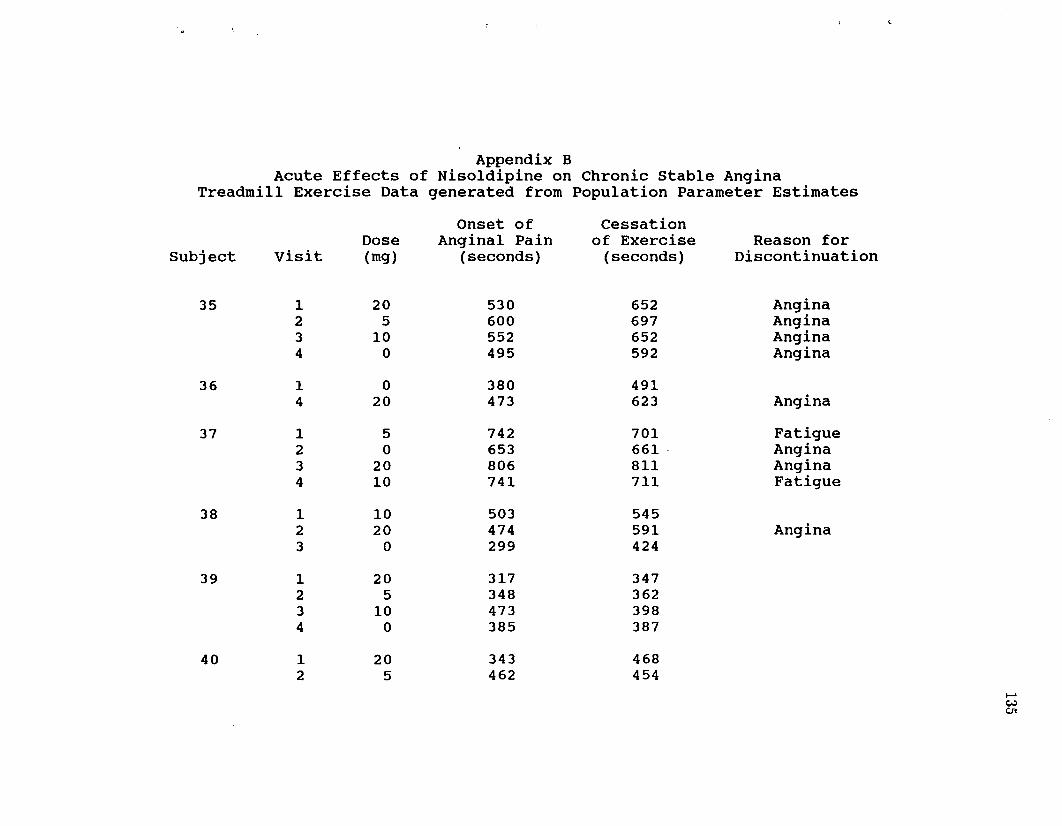
Appendix BAcute Effects of Nisoldipine on Chronic stable Angina
Treadmill Exercise Data generated from Population Parameter Estimates
Onset of CessationDose Anginal Pain of Exercise Reason for
SUbject Visit (mg) (seconds) (seconds) Discontinuation
35 1 20 530 652 Angina2 5 600 697 Angina3 10 552 652 Angina4 0 495 592 Angina
36 1 0 380 4914 20 473 623 Angina
37 1 5 742 701 Fatigue2 0 653 661 . Angina3 20 806 811 Angina4 10 741 711 Fatigue
38 1 10 503 5452 20 474 591 Angina3 0 299 424
39 1 20 317 3472 5 348 3623 10 473 3984 0 385 387
40 1 20 343 4682 5 462 454
.....CJ,)01

Appendix BAcute Effects of Nisoldipine on Chronic stable Angina
Treadmill Exercise Data generated from Population Parameter Estimates
Onset of CessationDose Anginal Pain of Exercise Reason for
subject Visit (mg) (seconds) (seconds) Discontinuation
3 10 468 4534 0 320 318
41 2 5 535 613 Angina3 10 414 5424 0 354 434
42 1 0 553 580 Angina2 10 549 533 Fatigue3 5 324 4644 20 518 609 . Angina
43 1 10 509 5442 20 405 490
44 2 10 575 473 Fatigue3 5 391 3864 20 614 624 Angina
45 1 20 457 595 Angina2 5 475 5293 10 542 655 Angina4 0 559 616 Angina
46 1 10 593 592 Fatigue......w0)
~

~
Appendix BAcute Effects of Nisoldipine on Chronic stable Angina
Treadmill Exercise Data generated from Population Parameter Estimates
Onset of CessationDose Anginal Pain of Exercise Reason for
Subject Visit (mg) (seconds) (seconds) Discontinuation
3 0 493 4464 5 617 600 Fatigue
47 1 10 462 4953 0 401 476
48 1 20 588 657 Angina2 5 664 678 Angina3 10 480 4894 0 664 685 Angina
49 1 10 312 3472 20 237 3153 0 104 1964 5 202 274
50 1 20 91 1872 5 45 443 10 150 1734 0 73 40
51 1 5 513 603 Angina2 0 466 5293 20 575 642 Angina
......~
-1

Appendix BAcute Effects of Nisoldipine on Chronic stable Angina
Treadmill Exercise Data generated from Population Parameter Estimates
Onset of CessationDose Anginal Pain of Exercise Reason for
SUbject Visit (mg) (seconds) (seconds) Discontinuation
52 1 10 544 515 Fatigue2 20 385 4913 0 323 428
53 1 20 548 5512 5 409 4214 0 436 408
54 1 20 438 5354 0 195 281
55 1 0 324 4042 10 542 539 Fatigue3 5 480 526
56 1 20 773 814 Angina2 5 623 744 Angina3 10 633 689 Angina4 0 591 644 Angina
57 1 20 301 4142 5 379 4513 10 272 3554 0 265 432
......w(Xl
• ..

Appendix BAcute Effects of Nisoldipine on Chronic stable Angina
Treadmill Exercise Data generated from Population Parameter Estimates
Onset of CessationDose Anginal Pain of Exercise Reason for
SUbject Visit (mg) (seconds) (seconds) Discontinuation
58 1 0 367 3992 10 518 612 Angina4 20 600 596 Fatigue
59 1 0 412 4912 10 483 5423 5 455 5084 20 428 462
60 1 20 326 4093 10 412 4604 0 341 474
61 1 20 268 3972 5 291 3943 10 349 4584 0 210 354
62 1 20 575 690 Angina2 5 678 782 Angina3 10 645 693 Angina4 0 553 608 Angina
63 1 20 503 5492 5 516 499
.....~<0

Appendix BAcute Effects of Nisoldipine on Chronic stable Angina
Treadmill Exercise Data generated from Population Parameter Estimates
Onset of CessationDose Anginal Pain of Exercise Reason for
Subject Visit (mg) (seconds) (seconds) Discontinuation
3 10 438 4224 0 421 403
64 1 20 431 5212 5 560 607 Angina3 10 414 4874 0 502 533
65 1 0 645 722 Angina2 10 691 726 Angina3 5 594 670 Angina4 20 617 707 Angina
66 1 5 252 3052 0 215 242
67 1 10 492 5372 20 488 4873 0 358 3894 5 494 462
68 1 20 546 672 Angina3 10 477 572 Angina4 0 520 578 Angina
.....tJ::..0
, • '.

Appendix BAcute Effects of Nisoldipine on Chronic stable Angina
Treadmill Exercise Data generated from population Parameter Estimates
Onset of CessationDose Anginal Pain of Exercise Reason for
SUbject Visit (mg) (seconds) (seconds) Discontinuation
69 1 5 532 4682 0 359 4154 10 621 554 Fatigue
70 1 5 593 636 Angina2 0 469 5533 20 507 618 Angina
71 1 0 550 541 Fatigue2 10 534 609 Angina3 5 495 5504 20 619 680 Angina
72 1 0 541 540 Fatigue2 10 650 602 Fatigue3 5· 548 547 Fatigue4 20 585 556 Fatigue
73 1 0 565 590 Angina2 10 540 5473 5 548 5564 20 506 513
74 1 10 395 4482 20 398 479
.....~.....

Appendix BAcute Effects of Nisoldipine on Chronic stable Angina
Treadmill Exercise Data generated from Population Parameter Estimates
Onset of CessationDose Anginal Pain of Exercise Reason for
SUbject Visit (mg) (seconds) (seconds) Discontinuation
3 0 203 3294 5 458 436
75 1 5 402 4242 0 297 3183 20 253 3794 10 415 428
76 1 0 309 3822 10 354 4043 5 178 334
77 1 10· 432 3552 20 434 4253 0 296 2874 5 392 412
78 1 0 374 3592 10 333 3523 5 41 1514 20 346 302
79 3 5 382 489
80 1 10 812 788 Fatigue~
~l'-j
*.. ·f
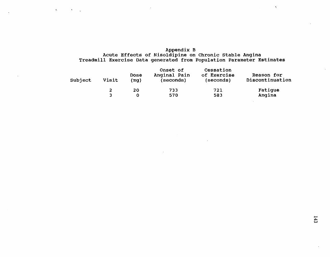
',-,c
Appendix BAcute Effects of Nisoldipine on Chronic stable Angina
Treadmill Exercise Data generated from Population Parameter Estimates
Onset of CessationDose Anginal Pain of Exercise Reason for
SUbject Visit (mg) (seconds) (seconds) Discontinuation
2 20 733 721 Fatigue3 0 570 583 Angina
~
>P0w

144
REFERENCES
Aitkin, M. (1981), "A Note on the Regression Analysis of Censored Data,"Technometrics, 23(2), 161-163.
Batchelor, J. R., and Hackett, M. (1970), "HL-A Matching in Treatment ofBurned Patients With Skin Allografts," The Lancet, 2, 581-583.
Beck, J. V., and Arnold, K. J. (1977), Parameter Estimation in En"ineering andScience, New York: Wiley.
Bissette, J., Carr, G., Koch, G. G., Adams, K. F., and Sheps, D. S. (1986),"Analysis of (Events/Time at Risk) Ratios From Two-Period CrossoverStudies," Proceedin"s of the Biopharmaceutical Section of the AmericanStatistical Association.
Breslow, N. (1974), "Covariance Analysis of Censored Survival Data," Biometrics,30, 89-99.
Carriquiry, A. L. (1985), "The Analysis of a Censored Multivariate NormalDistribution: Onset of Puberty in Mice," unpublished M.S. thesis, Universityof Illinois, Department of Animal Sciences.
Carriquiry, A. L., Gianola, D.,· and Fernando, R. 1. (1987), "Mixed-ModelAnalysis of a Censored Normal Distribution With Reference to AnimalBreeding," Biometrics, 43, 929-939.
Chaitman, B. R., Wagniart, P., Pasternac, A., Brevers , G., Scholl, J., Lam, J.,Methe, M., Ferguson, R., and Bourassa, M. G. (1984), "Improved ExerciseTolerance After Propranolol, Diltiazem, or Nifedipine in Angina Pectoris:Comparison at 1, 3, and 8 Hours and Correlation with Plasma DrugConcentration," The American Journal of Cardiology, 53(1), 1-9.
Chatterjee, S., and McLeish, D. L. (1986), "Fitting Linear Regression Models toCensored Data by Least Squares and Maximum Likelihood Methods,"Communications in Statistics :. Theory and Methods, 15(11), 3227-3243.
Cox, D. R., and Oakes, D. (1984), Analysis of Survival Data, New York: Chapmanand Hall.
Dempster, A. P., Laird, N. M., and Rubin, D. B. (1977), "Maximum LikelihoodFrom Incomplete Data via the EM Algorithm," Journal of the RoyalStatistical Society, B, 39, 1-38.
Elandt-Johnson, R. C., and Johnson, N. 1. (1980), Survival Models and DataAnalysis, New York: Wiley.
Fairclough, D. 1., and Helms, R. W. (1984), "Mixed Effects Model Analyses ofIncomplete Longitudinal Pulmonary Function Measurements in Children,"Institute of Statistics Mimeo Series No. 1470, University of North Carolina atChapel Hill.
•

145
Harville, D. A. (1974), "Bayesian Inference for Variance Components Using OnlyError Contrasts," Biometrika, 61, 383-385.
____ (1976), "Extension of the Gauss-Markov Theorem to Include theEstimation of Random Effects," The Annals of Statistics, 4(2), 384-395.
____ (1977), "Maximum Likelihood Approaches to Variance ComponentEstimation and to Related Problems," Journal of the American StatisticalAssociation, 72 (358), 320-338.
Helms, R. W. (1988), "Manipulating Statistical Hypotheses and Tests as BooleanFunctions," The American Statistician, 42, 253-256.
Kalbfleisch, J. D., and Prentice, R. L. (1980), The Statistical Analysis of FailureTime Data, New York: Wiley.
Kotz, S., and Johnson, N. L. (1983), Encyclopedia of Statistical Sciences (Vol. 4),New York: Wiley.
Laird, N. M., and Ware, J. H. (1982), "Random-Effects Models for LongitudinalData," Biometrics, 38, 963-974.
Lam, J., Chaitman, B. R., Crean, P., Blum, R., and Waters, D. D. (1985), "ADose-Ranging, Placebo-Controlled, Double-Blind Trial of Nisoldipine inEffort Angina: Duration and Extent of Antianginal Effects, "Journal of theAmerican College of Cardiology, 6(2), 447-452.
Lawless, J. F. (1982), Statistical Models and Methods for Lifetime Data, NewYork: Wiley.
Little, R. J. A., and Rubin, D. B. (1987), Statistical Analysis with Missing Data,N:ew York: Wiley.
McCarroll, K., and Helms, R. W. (1987), "An Evaluation of Some Approximate FStatistics and Their Small Sample Distributions for the Mixed Model WithLinear Covariance Structure," Institute of Statistics Mimeo Series No. 1838T,University of North Carolina at Chapel Hill.
Murray, S. C., and Helms, R. W. (1990), "Linear Models with Generalized AR(l)Covariance Structure for Irregularly-Timed Data," Institute of StatisticsMimeo Series No. 1876, University of North Carolina at Chapel Hill.
Naughton, J., and Haider, R. (1973), Methods of Exercise Testing. In: Naughton,J. P., Hellerstein, H. K., and Mohler, I. C., eds. Exercise Testing andExercise Training in Coronary~ Disease, New York: Academic Press,79-91.
Neyman, J., and Scott, E. L. (1948), "Consistent Estimates Based on PartiallyConsistent Observations," Econometrica 16(1), 1-32.
Pettitt, A. N. (1986), "Censored Observations, Repeated Measures and MixedEffects Models: An Approach Using the EM Algorithm and Normal Errors,"Biometrika 73(3), 635-643.

146
Sampford, M. R., and Taylor, J. (1959), "Censored Observations in RandomizedBlock Experiments," Journal of the R2W Statistical Society, B, 21, 214-237.
Schluchter, M. D. (1991), "Methods for the Analysis of Informatively CensoredLongitudinal Data," presented at the Symposium on Longitudinal DataAnalysis, Sponsored by the Biopharmaceutical Section of the AmericanStatistical Association, Fort Lauderdale, Florida.
Schmee, J., and Hahn, G. J. (1979), "A Simple Method for Regression AnalysisWith Censored Data," Technometrics, 21(4), 417-432.
Searle, S. R. (1982), Matrix Algebra Useful for Statistics, New York: Wiley.
Swan, A. V. (1969a), "Maximum Likelihood Estimation From Grouped andCensored Normal Data," Algorithm AS 16, Applied Statistics, 18, 110-114.
____ (1969b), "The Reciprocal of Mills's ratio," Algorithm AS 17, AppliedStatistics, 18, 115-116. .
____ (1977), "A Remark on AS 16," Applied Statistics, 26, 122.
Timm, N. H. (1970), "The Estimation of Variance-Covariance and CorrelationMatrices from Incomplete Data," Psychometrika, 35, 417-437.
Ware, J. H. (1985), "Linear Models for the Analysis of Longitudinal Studies," TheAmerican Statistician, 39(2), 95-101.
•
Wei, L. J., Lin, D. Y., and Weissfeld, L.Multivariate Incomplete Failure TimeDistributions," Journal of the American1065-1073.
(1989), "Regression Analysis ofData by Modeling Marginal
Statistical Association, 84(408),
Wolynetz, M. S. (1974),"Analysis of Type I Censored - Normally DistributedData," unpublished Ph.D. dissertation, University of Waterloo, Departmentof Statistics and Actuarial Science.
____ (1979a), "Maximum Likelihood Estimation From Confined and CensoredNormal Data," Algorithm AS 138, Applied Statistics, 28, 185-195.
____ (1979b), "Maximum Likelihood Estimation in a Linear Model FromConfined and Censored Normal Data," Algorithm AS 139, Applied Statistics,28, 195-206.
Wolynetz, M. S., and Binns, M. R. (1983), "Stayablilty of Dairy Cattle: Modelswith Censoring and Covariates," Journal of Dairy Science, 66, 935-942.
Wu, M. C., and Bailey, K. R. (1989), "Estimation and Comparison of Changes inthe Presence of Informative Right Censoring: Conditional Linear Model,"Biometrics, 45, 939-955.
____ (1989), "Analysing Changes in the Presence of Informative Right CensoringCaused by Death and Withdrawal," Statistics in Medicine, 7, 337-346.
147
Wu, M. C., and Carroll, R. J. (1988), "Estimation and Comparison of Changes inthe Presence of Informative Right Censoring by Modeling the CensoringProcess," Biometrics, 44, 175-188.
Zeger, S. L., Liang, K.-Y., and Albert, P. S. (1988), "Models for LongitudinalData: A Generalized Estimating Equation Approach," Biometrics, 44, 10491060.
Zellner, A. (1971), An Introduction to Bayesian Inference in Econometrics, NewYork: Wiley.
Top Related