


Languages
Pages
Legal

Very Preliminary and IncompletePlease do not quote
OLIGOPOLY, DISCLOSURE AND EARNINGS MANAGEMENT∗
by
Mark Bagnoliand
Susan G. Watts
Krannert Graduate School of ManagementPurdue University
West Lafayette, IN 47907
Current Draft: May 2007
∗ We thank Hsin–Tsai Liu for her invaluable research assistance and gratefully acknowledge the
financial support provided by the Krannert Graduate School of Management and Purdue Univer-
sity.
1. Introduction.
C. Michael Armstrong, former CEO of AT&T, has recently argued that accounting fraud
at Worldcom was the cause of AT&T’s perceived strategic failures, its inability to compete with
Worldcom and, in the end, the decision to break up the company. More specifically, Armstrong has
argued that Worldcom’s fraudulently reported revenues, margins and costs drove AT&T’s layoffs,
cost cutting and a very unprofitable price war that left the company unable to service its debt.
His view of the impact of Worldcom’s accounting on competitors is also held by former Sprint
CEO William Estry.1 Motivated by these arguments, we develop a model designed to enhance
our understanding of how firms can obtain a competitive advantage by biasing disclosures made
in their financial statements.
We employ an incomplete information Cournot duopoly model in which each firm knows its
own production costs but not its rival’s. Each firm also provides a disclosure through, for example,
its income statement. The firm’s rival can use the disclosure to update its beliefs about the
disclosing firm’s production costs prior to competing in the product market. Our model differs
from prior work on disclosure in incomplete information Cournot models because we assume that
firms can provide biased reports. However, if they do so, they incur a cost of misreporting.2 We
show that when the firms know each other’s cost of misreporting, there are no linear equilibria.
However, when these costs are also private information, there are linear equilibria in which the
firms bias their disclosures to gain a competitive advantage in the product market.
In particular, each firm’s disclosure is designed to imply that its production costs are lower
than they actually are. Further, because each firm uses all available information efficiently and
fully understands their rival’s incentives to bias its report, each adjusts its beliefs about its rival’s
production costs upward relative to the disclosure but, in equilibrium, still underestimates those
costs. Consequently, each firm cuts its production below the full–information level causing the
market price to rise and each firm’s product market profits to increase, providing just the incentive
needed for each firm to bias its disclosure. Said differently, in our model, each firm engages in
1 See, for example, the recent book by Martin [2004], the former head of public relations at AT&T, or thearticles by Searcy [2005], Blumenstein and Grant [2004] and McConnell et al [2002].
2 The literature in this area includes Fried [1984], Shapiro [1986], Gal–or [1988, 1996], Darrough [1993], Raith[1996] and Vives [2002]. See, also, the survey by Verrecchia [2001]. When the authors in this literature focuson disclosure, the assumption is that the firms’ disclosures are unbiased but that the firms can determine theamount of noise in the disclosure. Thus, if the firm wishes to disclose, it chooses not to add noise and if itwishes not to disclose, it chooses to add an infinite amount of noise.
1
earnings management that results in a downwardly biased estimate of its production cost.3 Our
analysis indicates that these effects are smaller when the firms compete in more profitable product
markets or when they use reasonably similar technologies. Interestingly, while the effects are
smaller in both cases, they differ in that firms engage in more (less) misreporting in the first
(second) situation. Finally, when firms have different costs of misreporting, the firm with the
lower costs introduces greater bias into its reports, produces more output than it would in the
full information outcome and earns greater product market profits. Thus, our analysis supports
Armstrong’s view of the competitive impact of Worldcom’s fraudulent accounting and suggests
that it may be worth examining similar competitive environments for similar activity.
By focusing on equilibrium incentives to bias reports, our analysis suggests new empirical im-
plications associated with the use of different earnings management techniques. First, as mentioned
in footnote 3, only some techniques can effectively bias inferences about the firm’s production costs.
Thus, our model predicts that the use of these techniques is positively correlated with standard
measures of profitability such as ROE. Further, we expect that firms that have similar production
technologies will be less likely to employ these types of earnings management techniques. Thus,
firms whose production is governed by physical or chemical processes or firms in mature industries
are less likely to engage in this type of earnings management than firms in service industries or
firms that have significantly larger portfolios of products. Finally, our analysis suggests that the
increased use of deferred prosecution agreements (DPAs) is likely to lead to unexpected conse-
quences. In particular, because such agreements dramatically increase the cost of misreporting,
the competitors of firms operating under DPAs are likely to respond by increasing the amount of
misreporting in order to gain/increase their competitive advantage in the product market.
The literature on the interaction between disclosures and product market competition was
extended and synthesized in Darrough [1993] and subsequently generalized in Raith [1996]. The
key difference between this literature and our model is that prior work required firms to make
unbiased disclosures—firms could only alter the amount of noise in their disclosure—whereas we
permit firms to bias their disclosures at a cost which leads to very different predictions. For
Cournot competitors with private information about production costs, Darrough and others have
3 Examples of this type of earnings management include fraudulent revenue recognition, aggressive cost cap-italization, inclusion of operating costs in restructuring costs, inappropriately low estimates of the allowancefor doubtful accounts or warranty expense, and certain types of “real” earnings management such as delayingexpenditures. Examples of earnings management techniques that would not lead to biased inferences aboutproduction costs include channel stuffing, delayed write–downs of assets, and the “timely” sale of assets.
2

shown that firms prefer to precommit to disclosing their private information without adding any
noise. Intuitively, adding noise results in the firm’s rival choosing to produce more than it would
if fully informed which lowers price and product market profits. If the disclosure decision is made
after the firms learn their production costs then, because they are required to disclose truthfully,
the standard unraveling story holds.4 Our results complement the prior literature by showing that
when firms are permitted to bias disclosures (even at a cost), they choose to do so and that this
decision is affected by and affects competition in the product market.5
The remainder of the paper is organized as follows. Section 2 contains a description of our
model of disclosure and product market competition and describes the equilibrium. In Section 3,
we focus on symmetric equilibria and analyze asymmetric equilibria in Section 4. We conclude in
Section 5.
2. The Model and Equilibrium.
We examine a two–stage game designed to capture the interaction between a firm’s disclosure,
earnings management and its competitive position in its product market. In the first stage, each
of two firms chooses a disclosure without knowing its rival’s choice and incurs a disclosure cost.
Each firm makes this disclosure knowing both its own disclosure and production costs. As a result,
the disclosure may provide information about the firm’s cost of production and may therefore be
of use to its rival when the two firms compete in their product market. In the second stage of the
game, the firms observe both disclosures from the first stage and compete in the product market
by choosing an amount of the homogeneous product to offer for sale without observing the output
choice of its rival. We simplify the analysis by assuming that each firm has constant marginal
costs of production and fixed costs are zero. Together, these imply that the firm’s average costs of
production equal its marginal costs.
More specifically, in the disclosure stage of our game, each firm chooses a disclosure which we
interpret as a disclosure about the firm’s average cost of production. Our objective is to capture
4 See Christensen and Feltham [2002] for a nice summary of this literature. Interestingly, in a recent paper,Arya, Frimor and Mittendorf [2007] have shown that if the firms compete in multiple markets, the unravelingresult may fail. In particular, they show that there can be a partial pooling equilibrium in which firm typesthat have high costs in one market and low costs in the other pool with firm types with low costs in the firstand high costs in the second.
5 The issue of whether the firms precommit to disclose does not arise substantively in our model because thefirms have the ability to select a disclosure that is independent of their private information. Thus, even if thefirms precommit to disclose, they have an available strategy that allows them to reveal none of their privateinformation.
3
the idea that a firm’s financial statement information (e.g., an income statement) can be used to
infer the firm’s reported marginal/average costs. Further, since firms can make reporting decisions
that either enhance or diminish reported earnings (both within the discretion afforded by GAAP
and/or through fraud), we do not require that the firm disclose truthfully. Instead, we assume
that if it does not disclose truthfully, it incurs a disclosure cost hi(si, ci), i = 1, 2 where si is
firm i’s disclosure and ci is its cost of production. To keep the analysis tractable, we assume
that hi(si, ci) = ki(si − ci) + (1/2)εi(si − ci)2 with εi > 0. Notice that with this specification,
firms that disclose truthfully incur no disclosure costs but firms that do not to disclose truthfully
incur two types of costs. The first type (represented by the second term) imposes a quadratic
cost of misreporting ci—if the firm misreports (si �= ci), it incurs a cost that is proportional to
the squared difference between its disclosure and its actual marginal cost of production.6 As a
result, it is symmetric in deviations from disclosing truthfully. The second type of disclosure cost
(represented by the first term) is not symmetric and depends on the sign of ki. Intuitively, if
ki > 0, then the firm’s disclosure costs increase when its disclosure exceeds its actual marginal
cost of production and may represent an added disadvantage from the market inferring that it is
less competitive. Similarly, if ki < 0, the firm’s disclosure costs increase when its disclosure is
smaller than its actual marginal costs and may represent an added disadvantage associated with a
(perceived) weakened position in bargaining with employees or in dealing with regulators (Watts
and Zimmerman [1986, 1990]).
In the second stage of the game, the two firms observe the first–stage disclosures (s1, s2) and
compete in the product market. We model the product market using a fairly standard incomplete
information, Cournot duopoly model where firms know their own cost of production but do not
know their rival’s costs.7 More specifically, we assume that the market demand for the homogeneous
product sold by the two firms is P = a−Q where Q = q1 + q2 and units of output are normalized
so that the slope coefficient of the demand function is 1. All information about market demand is
common knowledge.
An important component of our model is the information structure. We assume that firm i
6 Quadratic cost functions have become relatively common in the disclosure literature because they are partic-ularly tractable. See, for example, Crawford and Sobel [1982], Fischer and Stocken [2001] and Chakrabortyand Harbaugh [2007] who employ a quadratic cost function in their models of cheap talk as well as the modelsin Stocken and Verrecchia [2004], Fischer and Stocken [2004] and Guttman et al. [2006].
7 Prior work using a Cournot model with incomplete information about costs include Fried [1984], Shapiro[1986], Gal–or [1988, 1996], Darrough [1993] and Vives [2002]. See also the survey on disclosure by Verrecchia[2001].
4
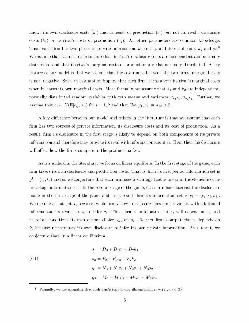
knows its own disclosure costs (ki) and its costs of production (ci) but not its rival’s disclosure
costs (kj) or its rival’s costs of production (cj). All other parameters are common knowledge.
Thus, each firm has two pieces of private information, ki and ci, and does not know kj and cj .8
We assume that each firm’s priors are that its rival’s disclosure costs are independent and normally
distributed and that its rival’s marginal costs of production are also normally distributed. A key
feature of our model is that we assume that the covariance between the two firms’ marginal costs
is non–negative. Such an assumption implies that each firm learns about its rival’s marginal costs
when it learns its own marginal costs. More formally, we assume that k1 and k2 are independent,
normally distributed random variables with zero means and variances σk1k1 , σk2k2 . Further, we
assume that ci ∼ N (E[ci], σii) for i = 1, 2 and that Cov[c1, c2] ≡ σ12 ≥ 0.
A key difference between our model and others in the literature is that we assume that each
firm has two sources of private information, its disclosure costs and its cost of production. As a
result, firm i’s disclosure in the first stage is likely to depend on both components of its private
information and therefore may provide its rival with information about ci. If so, then the disclosure
will affect how the firms compete in the product market.
As is standard in the literature, we focus on linear equilibria. In the first stage of the game, each
firm knows its own disclosure and production costs. That is, firm i’s first period information set is
y1i = (ci, ki) and so we conjecture that each firm uses a strategy that is linear in the elements of its
first stage information set. In the second stage of the game, each firm has observed the disclosures
made in the first stage of the game and, as a result, firm i’s information set is yi = (ci, si, sj).
We include si but not ki because, while firm i’s own disclosure does not provide it with additional
information, its rival uses si to infer ci. Thus, firm i anticipates that qj will depend on si and
therefore conditions its own output choice, qi, on si. Neither firm’s output choice depends on
ki because neither uses its own disclosure to infer its own private information. As a result, we
conjecture that, in a linear equilibrium,
s1 = D0 + D1c1 + D2k1
s2 = F0 + F1c2 + F2k2(C1)
q1 = N0 + N1c1 + N2s1 + N3s2
q2 = M0 + M1c2 + M2s1 + M3s2.
8 Formally, we are assuming that each firm’s type is two–dimensional, ti = (ki, ci) ∈ R2.
5
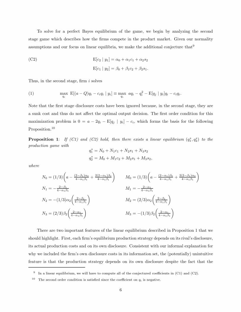
To solve for a perfect Bayes equilibrium of the game, we begin by analyzing the second
stage game which describes how the firms compete in the product market. Given our normality
assumptions and our focus on linear equilibria, we make the additional conjecture that9
E[c2 | y1] = α0 + α1c1 + α2s2(C2)
E[c1 | y2] = β0 + β1c2 + β2s1.
Thus, in the second stage, firm i solves
(1) maxqi
E[(a− Q)qi − ciqi | yi] ≡ maxqi
aqi − q2i − E[qj | yi]qi − ciqi.
Note that the first stage disclosure costs have been ignored because, in the second stage, they are
a sunk cost and thus do not affect the optimal output decision. The first order condition for this
maximization problem is 0 = a − 2qi − E[qj | yi] − ci, which forms the basis for the following
Proposition.10
Proposition 1: If (C1) and (C2) hold, then there exists a linear equilibrium (q∗1 , q∗2) to theproduction game with
q∗1 = N0 + N1c1 + N2s1 + N3s2
q∗2 = M0 + M1c2 + M2s1 + M3s2,
where
N0 = (1/3)(
a − (2−β1)α04−α1β1
+ 2(2−α1)β04−α1β1
)M0 = (1/3)
(a − (2−α1)β0
4−α1β1+ 2(2−β1)α0
4−α1β1
)
N1 = − 2−β14−α1β1
M1 = − 2−α14−α1β1
N2 = −(1/3)α2
(2−β1
4−α1β1
)M2 = (2/3)α2
(2−β1
4−α1β1
)
N3 = (2/3)β2
(2−α1
4−α1β1
)M3 = −(1/3)β2
(2−α1
4−α1β1
)
There are two important features of the linear equilibrium described in Proposition 1 that we
should highlight. First, each firm’s equilibrium production strategy depends on its rival’s disclosure,
its actual production costs and on its own disclosure. Consistent with our informal explanation for
why we included the firm’s own disclosure costs in its information set, the (potentially) unintuitive
feature is that the production strategy depends on its own disclosure despite the fact that the
9 In a linear equilibrium, we will have to compute all of the conjectured coefficients in (C1) and (C2).
10 The second order condition is satisfied since the coefficient on qi is negative.
6
firm knows its own cost of production and uses it rather than its own disclosure to estimate its
rival’s marginal cost of production. As we suggested above, the reason for this dependence is that
firm i knows that its rival is using i’s disclosure to make inferences about i’s production costs (see
equations (C2)) and thus i can infer that its rival’s production strategy will depend on si. Since
firm i’s production strategy depends on its inference about firm j’s production decision which firm
i knows depends on si, i’s production strategy “indirectly” depends on its disclosure because of
the information its rival can extract from that disclosure. Second, the parameters describing the
equilibrium production strategies (the M ’s and N ’s) depend on the coefficients in the conditional
expectations described by (C2). Intuitvely, both firms are using all of their private information
and their public disclosures from the disclosure stage of the game to infer as much as they possibly
can about their rival’s production costs.
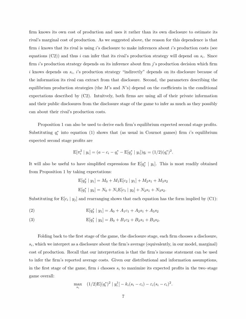
Proposition 1 can also be used to derive each firm’s equilibrium expected second stage profits.
Substituting q∗i into equation (1) shows that (as usual in Cournot games) firm i’s equilibrium
expected second stage profits are
E[π2i | yi] = (a − ci − q∗i − E[q∗j | yi])qi = (1/2)(q∗i )2.
It will also be useful to have simplified expressions for E[q∗j | yi]. This is most readily obtained
from Proposition 1 by taking expectations:
E[q∗2 | y1] = M0 + M1E[c2 | y1] + M2s1 + M3s2
E[q∗1 | y2] = N0 + N1E[c1 | y2] + N2s1 + N3s2.
Substituting for E[ci | yj ] and rearranging shows that each equation has the form implied by (C1):
E[q∗2 | y1] = A0 + A1c1 + A2s1 + A3s2(2)
E[q∗1 | y2] = B0 + B1c2 + B2s1 + B3s2.(3)
Folding back to the first stage of the game, the disclosure stage, each firm chooses a disclosure,
si, which we interpret as a disclosure about the firm’s average (equivalently, in our model, marginal)
cost of production. Recall that our interpretation is that the firm’s income statement can be used
to infer the firm’s reported average costs. Given our distributional and information assumptions,
in the first stage of the game, firm i chooses si to maximize its expected profits in the two–stage
game overall:
maxsi
(1/2)E[(q∗i )2 | y1i ]− ki(si − ci) − εi(si − ci)2.
7
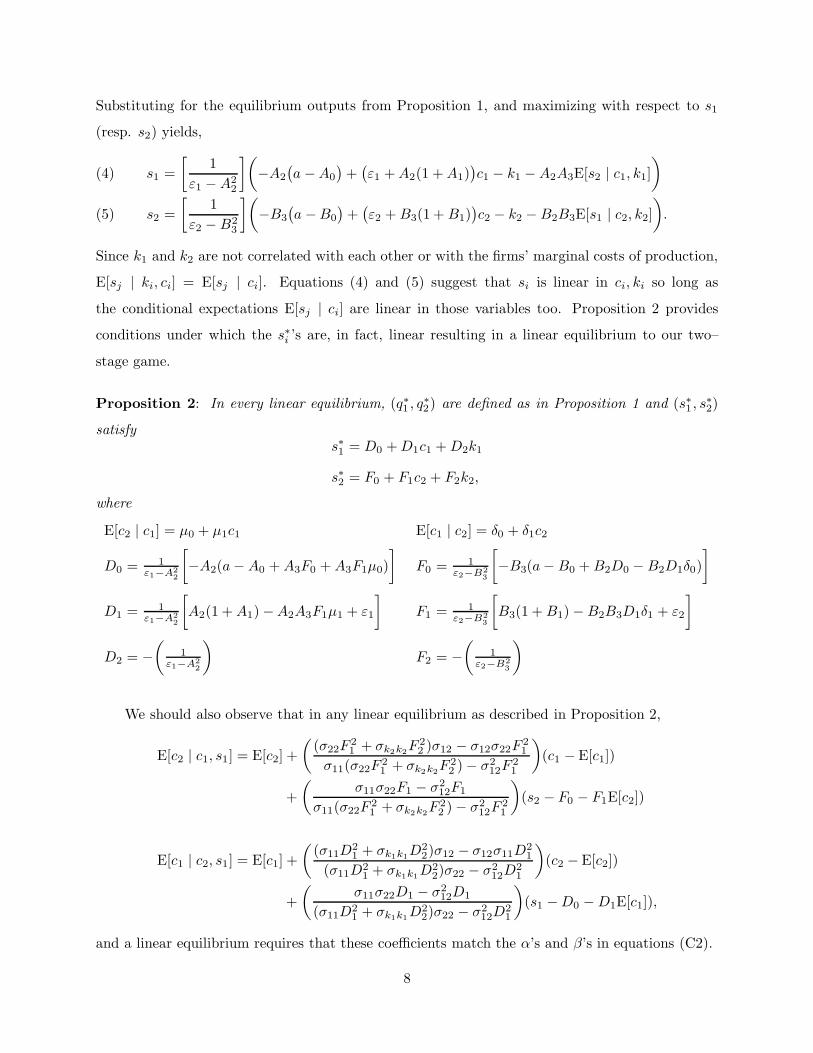
Substituting for the equilibrium outputs from Proposition 1, and maximizing with respect to s1
(resp. s2) yields,
s1 =[
1ε1 − A2
2
](−A2
(a −A0
)+
(ε1 + A2(1 + A1)
)c1 − k1 − A2A3E[s2 | c1, k1]
)(4)
s2 =[
1ε2 − B2
3
](−B3
(a −B0
)+
(ε2 + B3(1 + B1)
)c2 − k2 − B2B3E[s1 | c2, k2]
).(5)
Since k1 and k2 are not correlated with each other or with the firms’ marginal costs of production,
E[sj | ki, ci] = E[sj | ci]. Equations (4) and (5) suggest that si is linear in ci, ki so long as
the conditional expectations E[sj | ci] are linear in those variables too. Proposition 2 provides
conditions under which the s∗i ’s are, in fact, linear resulting in a linear equilibrium to our two–
stage game.
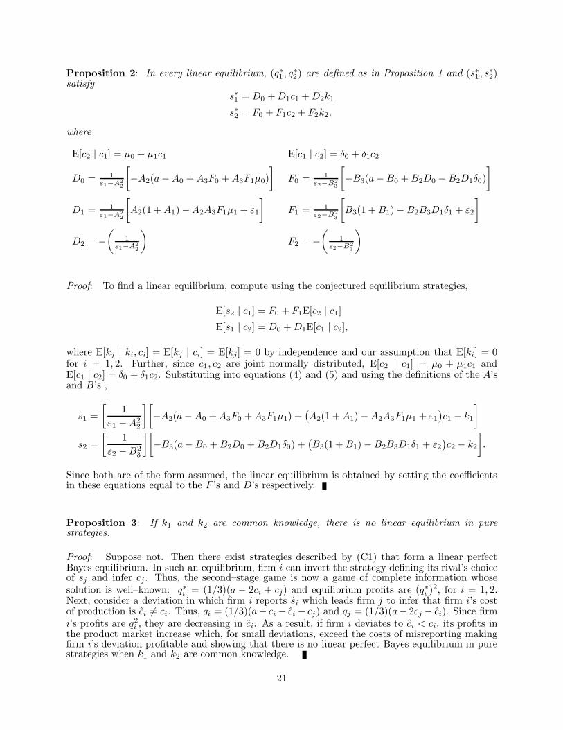
Proposition 2: In every linear equilibrium, (q∗1 , q∗2) are defined as in Proposition 1 and (s∗1 , s∗2)
satisfys∗1 = D0 + D1c1 + D2k1
s∗2 = F0 + F1c2 + F2k2,
where
E[c2 | c1] = μ0 + μ1c1 E[c1 | c2] = δ0 + δ1c2
D0 = 1ε1−A2
2
[−A2(a − A0 + A3F0 + A3F1μ0)
]F0 = 1
ε2−B23
[−B3(a − B0 + B2D0 − B2D1δ0)
]
D1 = 1ε1−A2
2
[A2(1 + A1) −A2A3F1μ1 + ε1
]F1 = 1
ε2−B23
[B3(1 + B1) − B2B3D1δ1 + ε2
]
D2 = −(
1ε1−A2
2
)F2 = −
(1
ε2−B23
)
We should also observe that in any linear equilibrium as described in Proposition 2,
E[c2 | c1, s1] = E[c2] +(
(σ22F21 + σk2k2F
22 )σ12 − σ12σ22F
21
σ11(σ22F21 + σk2k2F
22 ) − σ2
12F21
)(c1 − E[c1])
+(
σ11σ22F1 − σ212F1
σ11(σ22F21 + σk2k2F
22 ) − σ2
12F21
)(s2 − F0 − F1E[c2])
E[c1 | c2, s1] = E[c1] +(
(σ11D21 + σk1k1D
22)σ12 − σ12σ11D
21
(σ11D21 + σk1k1D
22)σ22 − σ2
12D21
)(c2 − E[c2])
+(
σ11σ22D1 − σ212D1
(σ11D21 + σk1k1D
22)σ22 − σ2
12D21
)(s1 −D0 − D1E[c1]),
and a linear equilibrium requires that these coefficients match the α’s and β’s in equations (C2).
8
Unfortunately, there is no general result on the existence of a perfect Bayes equilibrium in
this type of linear–normal model.11 Further, finding a linear equilibrium in closed form for our
model is very difficult because it requires solving a system of 24 non–linear equations for the
unknown coefficients. While numerical solutions can be obtained (and we do so below), in the next
subsection, we focus on symmetric equilibria and show that a linear equilibrium exists.
Before continuing, we should discuss the importance of our assumption that firm types are
two–dimensional. The easiest way to see the role of this assumption is to consider the effect of
assuming that both firms know the realizations of k1 and k2 (equivalently that σk1k1 = σk2,k2 = 0).
In this event, if the two firms adopt linear disclosure strategies, then each can invert their rival’s
strategy and infer their rival’s production costs from their rival’s disclosure. That is, if si is a
linear function of the only information that firm j does not know, ci, then firm j can infer the
realized value of ci from observing si. This turns the second–stage game into a game of complete
information since both firms now know their rival’s costs of production (and everything else is
common knowledge) and we are able to prove the following result:
Proposition 3: If k1 and k2 are common knowledge, there are no linear equilibrium in pure
strategies.
The key implication of assuming that k1 and k2 are common knowledge is that neither firm
can employ a linear disclosure strategy without revealing its actual production costs and, as a
result, there are no linear equilibria in pure strategies. To see why, note that each firm’s marginal
disclosure cost is approximately zero for small amounts of misreporting. Further, if firm i misleads
j into believing that i’s costs are lower than they actually are, it induces j to reduce its output
which allows firm i to increase its own output (in anticipation of j’s output choice). As a result,
product market profits are shifted from firm j to firm i. Thus, in any potential equilibrium in which
firm j believes that it can correctly infer firm i’s cost of production, firm i has incentives to mislead
thereby destroying the potential equilibrium. This analysis shows that our assumption that each
firm’s type is two–dimensional eliminates the possibility that each firm can infer its rival’s cost of
production from a linear disclosure strategy and, as a result, allows for the possibility of a linear
11 With minor modifications to our distributional assumptions however, the existence of a trembling handperfect Nash equilibrium ensures that there is a perfect Bayes equilibrium (see Fudenberg and Tirole [1993]).In particular, if each firm’s private information is drawn from a finite set (so that the set of types in our gameis finite), standard existence theorems ensure that there is a trembling hand perfect Nash equilibrium andtherefore a perfect Bayes equilibrium in the modified game.
9

equilibrium.12
3. Symmetric Equilibria.
In this subsection, we focus on symmetric equilibria and in the following subsection, we explore
the nature of asymmetric equilibria. In a symmetric equilibrium, both firms employ the same
strategies—the same map from their private information to their actions. Thus, the equilibrium
actions of the firms s1, s2 are determined by the same function of the firm’s private information
(c1, k1 and c2, k2 respectively) and the equilibrium production decisions q1, q2, are determined
by the same function of each firm’s information set (c1, s1, s2 and c2, s1, s2 respectively). That is,
symmetry requires that Di = Fi and αi = βi for i = 1, 2, 3; Ni = Mi for i = 1, 2, 3, 4 and μi = δi for
i = 1, 2. Further, we must assume that both firms are in the same “competitive position:” k1 and
k2 must be drawn from the same distribution, c1 and c2 must be drawn from the same distribution
and the firms must incur the same disclosure costs, ε1 = ε2 ≡ ε. Finally, without loss of generality,
we can simplify by assuming that all of the normally distributed random variables are standard
normal with zero means and variances equal to 1.13 Given this structure, we have
Proposition 4: If ε is not too small, there is a symmetric linear perfect Bayes equilibrium in pure
strategies.
Intuitively, if the cost of misreporting is sufficiently small we cannot support a linear equilib-
rium because each firm’s incentive to misreport is too great and thus cannot depend linearly on
the firm’s private information. However, if the cost of misreporting is not too small, then there is
a linear perfect Bayes equilibrium in which each firm provides a disclosure. The disclosure allows
the firm’s rival to update its beliefs about the disclosing firm’s production costs but does not allow
it to infer exactly what those costs are. The update does, however, affect how the rival competes
with the disclosing firm in the product market.
To better understand the properties of the disclosure and its effects on product market com-
petition, we will generally do numerical comparative static analysis because of the complexity of
the equations defining the symmetric equilibrium. Before that, however, we begin with an intuitive
result that does not require numerical techniques.
12 In that sense, the role of the second dimension of a firm’s type in our model is similar to the role of noisetraders in Kyle models of market making (see Kyle [1998] or Bagnoli, Viswanathan and Holden [2001]).
13 Equivalently, we can transform to standard normal random variables.
10
Proposition 5: As the cost of misreporting gets large,
(i) the amount of misreporting declines,
(ii) each firm’s estimate of its rival’s cost of production becomes more accurate and
(iii) each firm’s output approaches the output it would make in a full–informationenvironment.
Proposition 5 tells us that as the cost of misreporting gets large, the equilibrium in the
product market converges to the complete information solution. The reason is that as the cost of
misreporting gets large, the firms do less and less making their disclosures more informative. Thus,
the uncertainty about the rival’s cost dissipates and competition in the product market approaches
the outcome when the firms are fully informed of their rival’s cost of production. Interestingly, this
result does not require that firms precommit to a disclosure or be required to disclose truthfully.
Instead, as the cost of misreporting rises, firm behavior converges to the full information solution
where each truthfully discloses its private information about its production costs.
To get a clearer picture of how the equilibrium varies with respect to the cost of misreporting,
the correlation between the firm’s costs of production and the size of the product market, we turn
to numerical comparative static analyses. Since hi(si, ci) = ki(si−ci)+(1/2)εi(si−ci)2, a positive
(negative) ki produces marginal incentives for the firm to report si < ci (si > ci). Thus, we do all
numerical analyses below assuming that the realized values of k1 and k2 are zero. Given this, we
begin by analyzing the equilibrium described above in more detail and the effects of an increase in
the cost of misreporting, ε.
Result 1: In equilibrium, each firm’s reported cost of production is smaller than its actual cost
of production, each firm’s output is smaller than the full–information quantity and each firm’s
estimate of its rival’s costs is smaller than its rival’s actual cost of production.14
This result tells us that we should expect firms to bias their reported costs downward in
an attempt to convince their rival that their costs are lower than they actually are. If they are
successful, their rival will optimally reduce the amount it sells in the product market causing
the price to be higher and resulting in greater profits for the misreporting firm. Each firm, in
equilibrium, is successful because neither can perfectly extract its rival’s cost of production from
14 Further, combining Result 1 with Proposition 5 implies that when the cost of misreporting increases, allof these differences shrink with reported costs converging to actual costs, output choices converging to thefull–information quantities and each firm’s estimate of its rival’s costs converging to its rival’s actual costs.
11
its reported costs and while each understands the equilibrium and adjusts their expectation of
their rival’s cost taking into account the rival’s incentive to report lower costs, the adjustment is
only partial. Thus, in equilibrium, their expectation, conditional on everything they know, is still
smaller than the rival’s actual cost of production.
These results differ markedly from those in the prior literature (as described in Darrough [1993]
or the generalization in Raith [1996]). Darrough proves that if the firm’s disclosure is required to
be a noisy but unbiased reflection of the firm’s private information about its cost of production,
in equilibrium, both firms would precommit to minimize the noise in the disclosure.15 That is,
they report their private information without bias. Other models permit firms to choose whether
to disclose after learning their production costs but require that a firm choosing to disclose do so
truthfully. This literature, summarized in Christensen and Feltham [2002], shows that the standard
unraveling result applies—in equilibrium, every firm type discloses because if more than one type
is pooled together, the type with the lowest production costs can increase profits by disclosing its
costs and inducing its rivals to reduce the quantities that they offer for sale. In our model, the firms
are not required to disclose truthfully but, if they report with a bias, they incur a cost associated
with misreporting. Our analysis shows that when firms have the option to bias their disclosure
(even at a cost), they will do so and that the effects are only partially accounted for by its rival.16
Interestingly, our analysis also shows how the opportunity to misreport earnings impacts the
profits each firm earns in the product market. In particular, we have
Result 2: In equilibrium, misreporting allows both firms to earn greater profits in the product mar-
ket than they would if each had complete information about their rival’s cost of production. Further,
the profits the firms earn in the product market decline as the cost of misreporting increases.
Intuitively, the type of earnings management we examine allows each firm to bias their dis-
closures in order to affect its rival’s inference about the its cost of production. Result 1 indicates
that the firms use this ability to misreport costs as being lower than they actually are. Upon
15 Formally, if the firm’s private information is ψi, it is required to disclose ψi = ψi + νi where νi is a normallydistributed random variable with mean 0 and variance chosen by the disclosing firm. If the firm wishes todisclose its private information, it selects a variance of zero and if it wishes not to disclose, it selects a varianceof infinity. In neither case, can the disclosing firm intentionally bias its disclosure.
16 In this sense, our paper is in the spirit of Fisher and Verrecchia [2000] who extend disclosure models byassuming that the manager’s objective function is not known to the market and show that the manager optsto bias his/her earnings report and that the market cannot fully adjust its expectation of firm value for thebias because of its uncertainty about the manager’s objective function.
12

observing the disclosure, the rival updates its beliefs about the firm’s costs using the disclosure
and what it knows about the disclosing firm’s incentives to bias but still ends up estimating that
the firm’s costs are lower than they actually are. As a result, the rival infers that the firm will
be producing more than it actually does and responds by reducing the quantity that it chooses to
produce. Consequently, earnings management results in both firms selling less than they would
had they known their rival’s costs but the associated price increase (from selling less) results in
each firm earning greater profits than they would with complete information about its rival’s costs.
Further, Result 1 tells us that as the cost of misreporting rises, the magnitude of the bias in the
firms’ reports declines. Thus, since both firms’ profits in the product market are greater the greater
the equilibrium amount of earnings management, increases in the cost of misreporting lower the
equilibrium amount of earnings management and therefore lower the profits each firm earns in
the product market. Further, if the costs of misreporting are non–pecuniary or are incurred by
management rather than the firm, Result 2 implies that earnings management actually increases
the liquidation value of the firm.
The clearest empirical implications flow from associating changes in the cost of misreporting
with changes in reporting regulations. For example, Section 302 of the Sarbanes–Oxley Act of
2002 (SOX) requires, among other things, that CEOs and CFOs (or persons performing equivalent
functions) personally certify in each quarterly and annual report, including transition reports that,
“...he or she has reviewed the report; based on his or her knowledge, the report does not contain
any untrue statement of a material fact or omit to state a material fact necessary in order to make
the statements made, in light of the circumstances under which such statements were made, not
misleading with respect to the period covered by the report; based on his or her knowledge, the
financial statements, and other financial information included in the report, fairly present in all
material respects the financial condition, results of operations and cash flows of the issuer as of,
and for, the periods presented in the report....”17 Such certification increases the manager’s costs
of misreporting and would be represented by an increase in ε in our model. Thus, our model
(Proposition 5 and Result 1) suggests the not surprising result that the impact of Section 302 is
to reduce the amount of misreporting but also the more surprising results that: (i) each firm’s
estimates of their rival’s costs increase and become more accurate and (ii) each firm produces
17 See “Certification of Disclosure in Companies’ Quarterly and Annual Reports,” Securities and ExchangeCommission 17 CFR PARTS 228, 229, 232, 240, 249, 270 and 274 [RELEASE NOS. 33-8124, 34-46427, IC-25722; File No. S7-21-02] RIN 3235-AI54, http://www.sec.gov/rules/final/33-8124.htm.
13

additional output. Thus, to the extent that misreporting of the type we consider is important to
the economy, our analysis suggests that SOX, Section 302, should have expanded gross domestic
product but reduced taxable profits and tax revenues.
More importantly, our analysis suggests that only certain types of misreporting are effective
means by which a firm creates a competitive advantage in its product market. In particular,
aggressive cost capitalization, including operating costs in restructuring costs, or selling previously
written off inventory are all means of producing financial statements that lead the firm’s rival to
infer that the firm’s costs are lower than they actually are. Further, changes in certain estimates
can also produce the same result. For example, a firm that reduces the allowance for doubtful
accounts (to increase earnings rather than because of changes in its customers’ credit–worthiness)
increases reported revenue relative to operating expenses and thus leads its rival to infer that the
reporting firm’s costs are lower than they actually are. Another example is reducing warranty
expense estimates (without an associated change in the reliability of the product) that directly
lowers reported operating expenses and misleads the firm’s rival in a similar manner. Finally,
certain methods of “real” earnings management such as delaying expenditures have the same
effect. There are, however, a variety of “standard” earnings management techniques that would
not create a competitive advantage of the type we examine. For example, aggressive revenue
recognition or granting lenient credit terms (or, more aggressively, channel stuffing) all produce
greater earnings (assuming gross margins are positive) but do not affect a rival’s ability to use the
firm’s financial statements to infer its costs. Similarly, delays in writing down assets, over–reserving
for contingencies or “timely” selling of assets are all means of managing earnings that also do not
alter the rival’s ability to infer costs. Thus, assuming that firms generally face similar incentives
to engage in the second class of earnings management techniques, our analysis suggests that SOX
will reduce the use of the first class of earnings management techniques relative to the second. As
a result, our model predicts that the observed proportion of the first class of earnings management
techniques among SEC enforcement actions will be smaller post–SOX.
Having analyzed the impact of earnings management on competition in the product market,
we can expand our understanding of the incentives to manage earnings by examining how changes
in the product market affect each firm’s willingness to misreport costs.
Result 3: When the firms compete in more profitable product markets, the magnitude of mis-
reporting is greater but the bias in the rival’s estimate of a firm’s cost of production is smaller
14

which, in turn, results in a smaller gain in equilibrium product market profits relative to the full
information level of profit.
Intuitively, Result 3 shows how the competitive environment in a firm’s product market affects
its incentives to engage in the type of earnings management we analyze. In particular, firms that
compete in more profitable product markets (markets with larger demand intercepts) bias their
reported earnings more because the benefits from inducing a rival to reduce output are greater.
What may be less obvious is that the induced bias in the rival’s expectation of the firm’s cost is
smaller. The reason for this is that we are holding the cost of misreporting, ε, constant. As the
profitability of the product market increases, each firm reports ever smaller costs which increases
the cost of misreporting. Thus, as product market profitability increases, the increase in the amount
of misreporting is tempered by the increasing costs of misreporting which, in net, allows its rival
to better estimate the firm’s true cost of production. Since the estimate is better, the impact of
misreporting on the rival’s output choice declines and the equilibrium outcome converges to the
full information solution.
An immediate implication of Result 3 is that both reported (actual) earnings are positively
(negatively) correlated with the magnitude of misreporting (of the type we examine). As a result,
our analysis predicts that most measures of profitability (e.g., Return on Equity, Return on Invested
Capital, Return on Sales, etc.) should be positively correlated with the magnitude of misreporting
but negatively correlated after adjusting for the amount of misreporting. Alternatively, Result 3
implies that firms in highly profitable markets should be those firms that are more often engaged
in and/or engage in more misreporting than firms in less profitable markets.
Result 4: The more information a firm can extract about its rival’s cost from knowing its own
cost, the smaller is the magnitude of the misreporting, the smaller is the induced bias in the rival’s
estimate of the firm’s cost and the smaller is the deviation from the full information level of output.
The amount of information a firm can extract about its rival’s costs from knowing its own costs
is “measured” by the covariance between the costs, σ12. In particular, the greater the covariance,
the greater is the reduction in the firm’s remaining uncertainty about its rival’s cost after observing
its own costs. The reduction in this uncertainty reduces the effectiveness of misreporting by offering
a biased report and the result is that the product market equilibrium is closer to the full information
outcome than it would be had the firms’ costs been less highly correlated.
15
Result 4 suggests that firms with more similar technologies, such as those controlled by physical
or chemical processes, should be expected to be less likely to engage in misreporting and, if they do
so, to do so in smaller amounts than firms whose technologies are more likely to be very different
(e.g., service industries). We would also expect that firms in mature industries such as the auto or
steel industries would also be less likely to engage in (or to do relatively less) misreporting than
firms in industries with large portfolios of products. The latter are more likely to be in industries in
which rivals have a more difficult time inferring its production costs from information about their
own due to the large portfolio of products. One may potentially be able to test this empirically by
relating misreporting to the number of business segments in the firm.
In summary, Results 1, 2, 3 and 4 show the full effect of firms exercising the option to bias
their reported costs. Results 1 and 2 show how a firm’s decision to bias its disclosure impacts
the competition in its product market and Results 3 and 4 show the feedback effect—how the
competitive environment in the firm’s product market affects its incentives to manage earnings.
4. Asymmetric Equilibria.
The results in the previous subsection provide significant new insight into the relationship
between product market competition and misreporting designed to bias rival’s inferences about
the reporting firm’s cost of production. The one feature that cannot be explored when the focus
is on symmetric equilibria is the impact of differential costs of misreporting.
To do so, recall that in the prior analysis, we took εi to be the cost of misreporting and
implicitly treated it as either non–random or as the expected cost of misreporting.18 The advantage
of interpreting this as an expected cost is that there are now good reasons why firms would face
different expected costs of misreporting. Not only might firms differ in the likelihood that they
are examined for misreporting; it is also possible that firms are run by managers who differ in
their concern about the impact of being detected misreporting. This situation appears to apply
in the AT&T, Worldcom example cited in the introduction. To explore the effect of firms facing
different costs of misreporting, we turn to an examination of asymmetric equilibria. We again apply
numerical techniques because of the difficulties in solving the large system of non–linear equations
that describe the equilibrium in our model. The key difference is that we relax the assumption
18 If we assume that the cost of misreporting is uncorrelated with the firm’s private information, then becausethe firm’s payoffs are linear in that cost, we could take expectations with respect to it and simply replace therandom variable with its expectation in the expressions derived above.
16
that ε1 = ε2 by assuming, without loss of generality, that ε2 > ε1. And, as in the prior subsection,
we do all numerical analyses assuming that the realized values of k1 and k2 are zero.
Result 5: As ε2 rises relative to ε1:
(i) the amount of misreporting by the low cost misreporter increases while the amount ofmisreporting by the high cost misreporter declines,
(ii) the bias in the estimate of the low cost misreporter is greater but both converge tozero as ε2 rises
(iii) the low cost misreporter produces more output than the full information output whilethe high cost misreporter produces less and
(iv) the low cost misreporter earns greater product market profits than the high costmisreporter does and the difference increases as ε2 increases.
Result 5 describes how differences in the costs of misreporting affect competition. In particular,
the greater the difference in the firms’ costs of misreporting, the larger (smaller) is the amount done
by the low cost (high cost) misreporter. Thus, holding the lower cost of misreporting constant,
Result 5 suggests that increases in the higher cost firm’s costs motivates its rival to do more
misreporting. In fact, Result 5 says even more: If the low cost rises slower than the high cost, the
direct effect of the cost increase on the low cost misreporter (to reduce the amount of misreporting)
is overwhelmed by the indirect, competitive effect of the increase in its rival’s cost of misreporting.
Further, the lower cost of misreporting offers the firm a competitive advantage in the product
market which it exploits by selling more output than its rival and earning greater profits.
Result 5 also suggests some empirically testable implications. First, it may be reasonable to
assume that firms that were “forced” to replace upper management in the wake of a misreporting
scandal are likely to face a competitive response from the firm’s rivals which results in the rivals
engaging in more misreporting, increasing production and shifting profits away from the firm that
changed upper level management. Second, it suggests a potential risk from using deferred prosecu-
tion agreements in misreporting cases.19 Such agreements increase (potentially dramatically) the
firm’s cost of misreporting and our Result 5 suggests that such agreements will produce unwanted
competitive responses from the firm’s rivals. In particular, the agreements will motivate the firm’s
19 Recent examples of the use of such agreements regarding misreporting of the type we examine include theBristol–Myers Squibb case (www.usdoj.gov/usao/nj/press/files/pdffiles/deferredpros.pdf); the PNC Financialcase (http://www.usdoj.gov/opa/pr/2003/June/03 crm 329.htm); the Computer Associates case(http://www.sec.gov/litigation/litreleases/lr18891.htm); and the AOL case(http://www.usdoj.gov/opa/pr/2004/December/04 crm 790.htm).
17
rivals to increase the amount of misreporting they do.
5. Conclusion.
In the past few years C. Michael Armstrong, former CEO of AT&T, has argued that AT&T’s
perceived strategic failures, its inability to compete with Worldcom and the decision to break
the company up were the result of accounting fraud at Worldcom. He suggests that Worldcom’s
“...revenues were false, margins were false, their costs were false...” and that this resulted in
layoffs, cost cutting and finally, the decision to break up AT&Tin order to service its debt. Former
Sprint CEO William Esrey suggests that his company also struggled with its inability to match
Worldcom’s performance and noted that: “It never dawned on us the base of their pricing was
fraud.”20 Motivated by these arguments, in this paper, we develop a model that illustrates how
firms can obtain a competitive advantage by biasing disclosures in financial statements.
We examine an incomplete information Cournot duopoly model in which the firms know their
own production costs but not their rival’s. In our model, firms provide a disclosure (e.g., an income
statement) that its rival can use to update its beliefs about the disclosing firm’s production costs
prior to competing in the product market. Our model differs from the prior literature in that we
allow firms to provide biased reports but, if they do so, they incur a cost of misreporting.21 We
show that when these costs of misreporting are common knowledge, there are no linear equilibria to
our disclosure/competition model because the linear disclosure strategy can be inverted to correctly
infer the rival’s production costs.
However, when each firm is uncertain about their rival’s cost of misreporting and these costs
are not too small, there is a linear equilibrium in which the firms bias their disclosures in order
to gain a competitive advantage in the product market.22 In particular, they bias their reported
costs downward. Further, even though the firms use all available information efficiently, fully
understand each other’s incentives and adjust their beliefs about their rival’s costs upward, they
20 See, for example, the recent book by Martin [2004], the former head of public relations at AT&T, or thearticles by Searcy [2005], Blumenstein and Grant [2004] or McConnell et al [2002]. Esrey is quoted in Searcy[2005].
21 The prior literature on disclosure and Cournot competition with imperfect cost information assumes that thefirms are required to provide unbiased reports of their costs but can choose to add varying amounts of noise.The main result in this literature is that the firms choose to disclose without noise (Darrough [1993] or Raith[1996] among others).
22 This result is reminiscent of Fisher and Verrecchia [2000]. They show that the introduction of uncertaintyabout the manager’s objective function alters the standard results in the voluntary disclosure literature inthat the manager in their model biases his/her earnings report and that the market cannot fully adjust itsexpectation of firm value for the bias because of its uncertainty about the manager’s objective function.
18
still underestimate those costs. As a result, each cuts production relative to the full information
level and each earns greater product market profits. Interestingly, these effects are smaller in more
profitable product markets even though the magnitude of misreporting increases. They are also
smaller when the firms use more similar production technologies. Finally, we show that when firms
have different (expected) costs of misreporting, the bias in the low cost misreporter’s disclosure is
greater than its rival’s and it produces more output than the full information quantity.
By focusing on competitive motives to bias reports, our analysis suggests some new empirical
implications. To see why, note that aggressive cost capitalization, fraudulent revenue recognition,
inappropriate estimates of the allowance for doubtful accounts or warranty expense are all exam-
ples of (one class of) earnings management techniques that lead to underestimates of the firm’s
production costs whereas other standard earnings management techniques (the second class) such
as channel stuffing, delayed write–downs of assets or “timely” sales of assets do not lead to mis–
estimated production costs. Since incentives to use the second class of earnings management
techniques are likely to be independent of the incentives to employ the first class, our model pre-
dicts that regulatory increases in the cost of misreporting (e.g., Section 302 of the Sarbanes–Oxley
Act of 2002) will result in a change in the distribution of observed earnings management techniques
(as, for example, among SEC enforcement actions). In particular, we expect a reduction in the use
of the first class of earnings management techniques relative to the use of the second class. Second,
our analysis suggests that standard measures of profitability will be positively correlated with the
use of the first class of earnings management techniques. Third, firms with more similar technolo-
gies (e.g., those for whom production is governed by physical or chemical processes or those used in
mature industries) will be less likely to employ this type of earnings management than firms with
less similar technologies (e.g., service industries or firms that produce a large variety of different
products).
Finally, when we examine asymmetric equilibria in which one firm’s costs of misreporting are
greater, we find that the results support Armstrong’s assertions about the impact of Worldcom’s
accounting fraud on its competitors. Interestingly, the analysis also suggests that the more frequent
use of deferred prosecution agreements may lead to unexpected consequences—providing the firm’s
competitors with incentives to misreport so as to bias estimates of their production costs down.
19
6. Appendix.
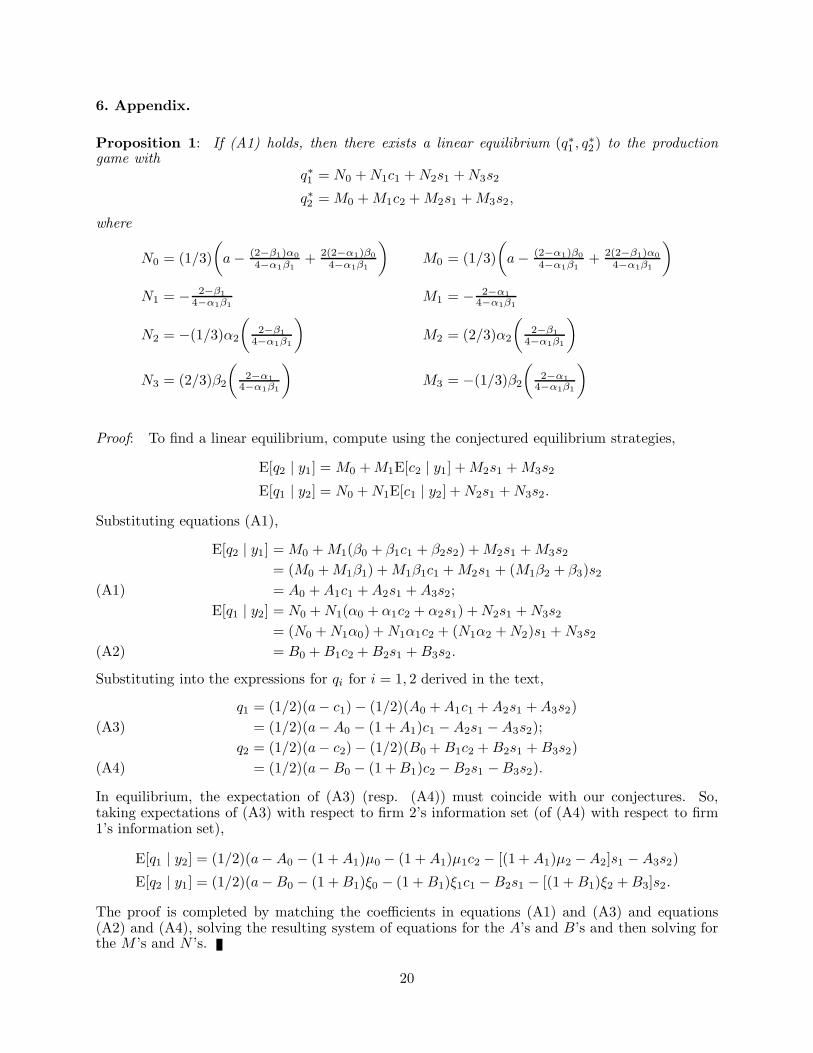
Proposition 1: If (A1) holds, then there exists a linear equilibrium (q∗1 , q∗2) to the productiongame with
q∗1 = N0 + N1c1 + N2s1 + N3s2
q∗2 = M0 + M1c2 + M2s1 + M3s2,
where
N0 = (1/3)(
a − (2−β1)α04−α1β1
+ 2(2−α1)β04−α1β1
)M0 = (1/3)
(a − (2−α1)β0
4−α1β1+ 2(2−β1)α0
4−α1β1
)
N1 = − 2−β14−α1β1
M1 = − 2−α14−α1β1
N2 = −(1/3)α2
(2−β1
4−α1β1
)M2 = (2/3)α2
(2−β1
4−α1β1
)
N3 = (2/3)β2
(2−α1
4−α1β1
)M3 = −(1/3)β2
(2−α1
4−α1β1
)
Proof: To find a linear equilibrium, compute using the conjectured equilibrium strategies,
E[q2 | y1] = M0 + M1E[c2 | y1] + M2s1 + M3s2
E[q1 | y2] = N0 + N1E[c1 | y2] + N2s1 + N3s2.
Substituting equations (A1),
E[q2 | y1] = M0 + M1(β0 + β1c1 + β2s2) + M2s1 + M3s2
= (M0 + M1β1) + M1β1c1 + M2s1 + (M1β2 + β3)s2
= A0 + A1c1 + A2s1 + A3s2;(A1)E[q1 | y2] = N0 + N1(α0 + α1c2 + α2s1) + N2s1 + N3s2
= (N0 + N1α0) + N1α1c2 + (N1α2 + N2)s1 + N3s2
= B0 + B1c2 + B2s1 + B3s2.(A2)
Substituting into the expressions for qi for i = 1, 2 derived in the text,
q1 = (1/2)(a− c1) − (1/2)(A0 + A1c1 + A2s1 + A3s2)= (1/2)(a− A0 − (1 + A1)c1 − A2s1 − A3s2);(A3)
q2 = (1/2)(a− c2) − (1/2)(B0 + B1c2 + B2s1 + B3s2)= (1/2)(a− B0 − (1 + B1)c2 −B2s1 −B3s2).(A4)
In equilibrium, the expectation of (A3) (resp. (A4)) must coincide with our conjectures. So,taking expectations of (A3) with respect to firm 2’s information set (of (A4) with respect to firm1’s information set),
E[q1 | y2] = (1/2)(a− A0 − (1 + A1)μ0 − (1 + A1)μ1c2 − [(1 + A1)μ2 −A2]s1 − A3s2)
E[q2 | y1] = (1/2)(a− B0 − (1 + B1)ξ0 − (1 + B1)ξ1c1 − B2s1 − [(1 + B1)ξ2 + B3]s2.
The proof is completed by matching the coefficients in equations (A1) and (A3) and equations(A2) and (A4), solving the resulting system of equations for the A’s and B’s and then solving forthe M ’s and N ’s.
20
Proposition 2: In every linear equilibrium, (q∗1 , q∗2) are defined as in Proposition 1 and (s∗1 , s∗2)
satisfys∗1 = D0 + D1c1 + D2k1
s∗2 = F0 + F1c2 + F2k2,
where
E[c2 | c1] = μ0 + μ1c1 E[c1 | c2] = δ0 + δ1c2
D0 = 1ε1−A2
2
[−A2(a − A0 + A3F0 + A3F1μ0)
]F0 = 1
ε2−B23
[−B3(a − B0 + B2D0 − B2D1δ0)
]
D1 = 1ε1−A2
2
[A2(1 + A1) −A2A3F1μ1 + ε1
]F1 = 1
ε2−B23
[B3(1 + B1) − B2B3D1δ1 + ε2
]
D2 = −(
1ε1−A2
2
)F2 = −
(1
ε2−B23
)
Proof: To find a linear equilibrium, compute using the conjectured equilibrium strategies,
E[s2 | c1] = F0 + F1E[c2 | c1]
E[s1 | c2] = D0 + D1E[c1 | c2],
where E[kj | ki, ci] = E[kj | ci] = E[kj] = 0 by independence and our assumption that E[ki] = 0for i = 1, 2. Further, since c1, c2 are joint normally distributed, E[c2 | c1] = μ0 + μ1c1 andE[c1 | c2] = δ0 + δ1c2. Substituting into equations (4) and (5) and using the definitions of the A’sand B’s ,
s1 =[
1ε1 −A2
2
][−A2(a − A0 + A3F0 + A3F1μ1) +
(A2(1 + A1) − A2A3F1μ1 + ε1
)c1 − k1
]
s2 =[
1ε2 −B2
3
][−B3(a − B0 + B2D0 + B2D1δ0) +
(B3(1 + B1) − B2B3D1δ1 + ε2
)c2 − k2
].
Since both are of the form assumed, the linear equilibrium is obtained by setting the coefficientsin these equations equal to the F ’s and D’s respectively.
Proposition 3: If k1 and k2 are common knowledge, there is no linear equilibrium in purestrategies.
Proof: Suppose not. Then there exist strategies described by (C1) that form a linear perfectBayes equilibrium. In such an equilibrium, firm i can invert the strategy defining its rival’s choiceof sj and infer cj . Thus, the second–stage game is now a game of complete information whosesolution is well–known: q∗i = (1/3)(a − 2ci + cj) and equilibrium profits are (q∗i )2, for i = 1, 2.Next, consider a deviation in which firm i reports si which leads firm j to infer that firm i’s costof production is ci �= ci. Thus, qi = (1/3)(a− ci − ci − cj) and qj = (1/3)(a− 2cj − ci). Since firmi’s profits are q2
i , they are decreasing in ci. As a result, if firm i deviates to ci < ci, its profits inthe product market increase which, for small deviations, exceed the costs of misreporting makingfirm i’s deviation profitable and showing that there is no linear perfect Bayes equilibrium in purestrategies when k1 and k2 are common knowledge.
21

Proposition 4: If ε is not too small, there is a symmetric linear perfect Bayes equilibrium in purestrategies.
Proof: In a symmetric equilibrium, Di = Fi and α1 = βi for i = 1, 2, 3; and Ni = Mi fori = 1, 2, 3, 4 and μi = δi for i = 1, 2. After matching coefficients, we have 12 non–linear equationsin 12 unknowns describing the coefficients of the firms’ strategies. By iterative substitution, oneobtains a a system of two equations in two unknowns, D1, D2 (resp. F1, F2). One equationis quadratic in D1 and has real roots when ε1(= ε2) is not too small. Solving for the roots andsubstituting into the other equation produces an 18th order polynomial in D2 with 87 sign changes.Thus, by Descartes’ Rule of Signs (see, for example, Levin [2002] and the references therein), thereis at least one real root and thus at least one symmetric linear equilibrium in pure strategies.
Proposition 5: As the cost of misreporting gets large, the amount of misreporting declines, eachfirm’s estimate of its rival’s cost of production becomes more accurate and each firm’s outputapproaches the output it would make in a full–information environment.
Proof: Suppose not, then in equilibrium, σi− ci > ξi > 0 for i = 1, 2 for all ε. Since E[πi | ki, ci] =E[(q∗i )2 | ki, ci] − hi(si, ci) and E[(q∗i )2] is bounded from above by the firm’s monopoly profits,[(a− ci)/2]2, if σi − ci > ξi > 0, then there is a ε large enough so that [(a− ci)/2]2 − hi(si, ci) < 0.Thus, if σi − ci > ξi > 0, there exists a large enough ε so that in the conjectured equilibrium, firmi’s expected profits are negative. Since firm i could deviate to si = ci and earn non-negative profits,such a deviation is profitable and we have shown that in every linear perfect Bayes equilibrium,σi − ci > ξi > 0 for all ε must be false. Given this, the difference si − ci must become arbitrarilysmall as ε gets large which implies that E[ci | cj , si, sj] − ci also becomes arbitrarily small asε becomes arbitrarily large. Finally, since q∗i is a linear function of ci and E[cj | ci, si, sj ] inequilibrium, it too converges to the complete information Cournot output as ε becomes arbitrarilylarge.
22
7. References.
Arya, A., H. Frimor and B. Mittendorf, 2007. “Aggregated Discretionary Disclosures in a Multi–Segment Firm,” working paper, The Ohio State University.
Bagnoli, M., S. Viswanathan and C. Holden, 2001. “On the Existence of Linear Equilibria inModels of Market Making,” Mathematical Finance, vol. 11 (1), 1–31.
Beneish, D., 2001. “Earnings Management: A Perspective,” Managerial Finance, vol. 27 (12),3–17.Blumenstein, R. and P. Grant, 2004. “On the Hook: Former Chief Tries to Redeem the Calls HeMade at AT&T— As He Retires, Armstrong Blames Industry Fraud for Breakup of Company —‘History Isn’t Always Right’,” Wall Street Journal, p. A1, May 26, 2004.
Chakraborty, A. and R. Harbaugh, 2007. “Comparative Cheap Talk,” Journal of Economic Theory,vol. 132 (1), 70–94.
Christensen, P., and G. Feltham, 2002. Economics of Accounting: Information in Markets,Springer, New York, NY.
Crawford, V. and J. Sobel, 1982. “Strategic Information Transmission,” Econometrica, vol. 50(6), 1431–1451.
Darrough, M., 1993. “Disclosure Policy and Competition: Cournot vs. Bertrand,” The AccountingReview, vol. 68 (3), 534–561.
Fischer, P. and P. Stocken, 2001. “Imperfect Information and Credible Communication,” Journalof Accounting Research, vol. 39 (1), 119–134.
Fischer, P. and P. Stocken, 2004. “Effect of Investor Speculation on Earnings Management,”Journal of Accounting Research, vol. 42 (5), 843–870.
Fried, D., 1984. “Incentives for Information Production and Disclosure in a Duopolistic Environ-ment,” Quarterly Journal of Economics, vol. 99 (2), 367–381.
Fudenberg, D. and J. Tirole, 1993. Game Theory, The MIT Press, Cambridge, Massachusetts.Gal–Or, E., 1988. “The Advantages of Imprecise Information,” Rand Journal of Economics, vol.19 (2), 266-275..
Gal–Or, E., 1986. “Information Transmission—Cournot and Bertrand Equilibria” Review of Eco-nomic Studies, vol. 53 (1), 85–92.
Guttman, I., O. Kadan and E. Kandel, 2006. “A Rational Expectations Theory of the Kink inAccounting Earnings,” The Accounting Review, vol. 81 (4), 811–848.
Healy, P., and K. Palepu, 2001. “Information Asymmetry, Corporate Disclosure and the CapitalMarkets: A Review of the Empirical Disclosure Literature,” Journal of Accounting & Economics,vol. 31 (1–3), 405–440.
Kyle, A., 1985. “Continuous Auctions and Insider Trading,” Econometrica, vol. 53 (6), 1315–1335.
Levin, S., 2002. “Descartes’ Rule of Signs — How Hard Can It Be?” Stanford University workingpaper.
Martin, D., 2004. Tough Calls: AT&Tand the Hard Lessons Learned from the Telecom Wars,AMACOM/American Management Association, New York, NY.
McConnell, B., J. Higgins, K. Kerschbaumer and P. Albiniak, 2002. “In the Loop,” Broadcastingand Cable Magazine, November 25, 2002.
Mulford, C. and E. Comiskey, 2002. The Financial Numbers Game, John Wiley and Sons, NewYork, NY.
Raith, M., 1996. “A General Model of Information Sharing in Oligopoly,” Journal of EconomicTheory, vol. 71 (2), 260–288.
23

Searcy, D., 2005. “Tracking the Numbers/Outside Audit: On Judgment Day, Assessing Ebbers’sImpact,” Wall Street Journal, p. C1, July 13, 2005.
Securities and Exchange Commission, 2002. Securities and Exchange Commission 17 CFR PARTS228, 229, 232, 240, 249, 270 and 274 [RELEASE NOS. 33-8124, 34-46427, IC-25722; File No. S7-21-02] RIN 3235-AI54, “Certification of Disclosure in Companies’ Quarterly and Annual Reports,”http://www.sec.gov/rules/final/33-8124.htm.
Shapiro, C., 1986. “Exchange of Information in Oligopoly,” Review of Economic Studies, vol. 53(3), 433–446.
Stocken, P. and R. Verrecchia, 2004. “Financial Reporting System Choice and Disclosure Manage-ment,” The Accounting Review, vol. 79 (4), 1181–1203.
Verrecchia, R., 2001. “Essays on Disclosure,” Journal of Accounting & Economics, vol. 32 (1–3),97–180.Vives, X., 2002. “Private Information, Strategic Behavior, and Efficiency in Cournot Markets,”Rand Journal of Economics, vol. 33 (3), 361–376.
Watts, R. and J. Zimmerman, 1986. Positive Accounting Theory, Prentice-Hall, London.
Watts, R. and J. Zimmerman 1990. “Positive Accounting Theory: A Ten Year Perspective,” TheAccounting Reviewvol. 65 (1), 131–156.
24
Top Related