


Languages
Pages
Legal

SUMMARY TABLES
Epicurus on Importance of Summaries Epicurus
01 Title Page
Chapter 1 INTRODUCTION AND BASIC CONCEPTS
02 Thermodynamics - Basic Concepts
03 Properties, Pressure Blaise Pascal
Chapter 2 ENERGY, ENERGY TRANSFER, AND GENERALENERGY ANALYSIS
04 Energy
05 Mechanical Energy, Energy Transfer
06 Heat and Work
07 The First Law of Thermodynamics James P. Joule vonMayer Epicurus
08 Energy Conversion Efficiences
Chapter 3 PROPERTIES OF PURE SUBSTANCES
09 Pure Substance, Phase, Phase Change Process, Property Diagrams
10 Property Tables
11 The Ideal-Gas Equation of State Robert Boyle JacquesCharles Joseph Louis Gay-Lussac
12 Compressibility Factor - A Measure of deviation from Ideal-gasBehavior
Chapter 4 ENERGY ANALYSIS OF CLOSED SYSTEMS
14 Moving Boundary Work
15 Polytropic Process
16 Energy Balance for Closed Systems
17 Specific Heats Joseph Black Joseph Black
17 Specific Heats - Solids and Liquids
Chapter 5 MASS AND ENERGY ANALYSIS OF CONTROLVOLUMES
18 Conservation of Mass
19 Flow Work
Energy Balance of Steady Flow
20 Steady-Flow Devices: Nozzles and Diffusers; Compressors, Turbines
Throttling Valves; Mixing Chambers; Heat Exchangers; Pipe Flow:Heaters, Condensors, Evaporators
21 Energy Analysis of Unsteady-Flow Systems
Chapter 6 THE SECOND LAW OF THERMODYNAMICS
22 Thermal Reservours, Heat Engines, Thermal Efficiency
24 Coefficient of Performance, Refrigerator, Heat Pump
23 The Second Law of Thermodynamics
25 The Carnot Cycle
Chapter 7 ENTROPY
26 Entropy
27 T-S Diagram
28 Gibbs Equation, Entropy Change
29 Reversible Steady-Flow Work
30 Isentropic Efficiences
31 Entropy Balance
Chapter 9 GAS POWER CYCLES
32 Gas Power Cycles - Basics
33 Reciprocating Engines - Overview

34 Otto Cycle
35 Diesel Cycle
36 Stirling and Ericsson Cycles
37 Brayton Cycle
Chapter 10 VAPOR AND COMBINED POWER CYCLES
38 Rankine Cycle
Chapter 11 REFRIGERATION CYCLES
39 Refrigeration Cycle

THERMODYNAMICSTHERMODYNAMICSTHERMODYNAMICSTHERMODYNAMICS
ME-321
Vladimir Soloviev

system
boundary
surroundings
THERMODYNAMICS All aspects of ENERGY and energy transformation (science of energy) Macro-thermodynamics (classical) matter is assumed to be continuum
Micro-thermodynamics (statistical) matter consists of discrete atoms
SYSTEM A region in space or a quantity of matter Open system (control volume) Closed system (control mass) Isolated system
PROPERTY Any characteristic of a system is called a property.
Intensive property mass-independent: { }T ,P, ,v,u,...ρ (lowercase letters)
Extensive property mass-dependent: { }m,V ,U ,E,... (upper case letters)
Specific property property per unit mass: { }v V m ,u U m ,e E m,...= = =
Independent properties { }T ,v ,{ }P,v ,{ }T,h ,…
STATE Set of all properties of the system defines a state { }T ,P,V ,m,u,e,v,s,h,...
EQUILIBRIUM Equilibrium is a state of balance. System can remain at equilibrium state indefinitely.
Thermodynamic equilibrium state: the system is in equilibrium regarding all possible changes of state; i.e. it maintains thermal, mechanical, phase, chemical etc. equilibria.
STATE POSTULATE The state of a simple compressible system is completely defined by two independent intensive properties PROCESS Change of a system from one state to another (transformation).
process diagram
Quasi-equilibrium process a system is close to equilibrium at any moment of process
Steady-flow process no change with time
Unsteady-flow process transient
Uniform no change with location
Iso-… process particular property remains constant (isothermal process)
cycle
heat
work
property 1
property 2
state
1State
path
2State
=1 2
heat
work
mass
Kazimir Malevich
The Black Square, 1915

PROPERTIES EXTENSIVE intensive
Mass m [ ]kg
Temperature T [ ]K
Pressure P [ ]kPa
Density m
Vρ =
3
kg
m
2H O
SGρ
ρ=
specific gravity (relative density)
Volume V 3m
V 1v
m ρ= =
3m
kg
specific volume
s
gγ ρ= 3
N
m
specific weight
Internal Energy U [ ]kJ U
um
= kJ
kg
specific internal energy
Total Energy E [ ]kJ E
em
= kJ
kg
specific total energy
Enthalpy H U PV= + [ ]kJ h u Pv= + kJ
kg
(heat content, total heat,“to heat”)
Specific heats p
c kJ
kg K
⋅ at constant pressure
v
c kJ
kg K
⋅ at constant volume
Entropy S kJ
K
s kJ
kg K
⋅
Quality vapor
liquid vapor
mx
m m=
+
quality is defined only for
saturated liquid-vapor mixtures
Blaise Pascale
( 1623 1662 )−
Pascal's Law
Manometer
h
fluid of
density ρ
oP P ghρ= +
o atmP P=
gas
Paris Museum of Measures and Arts
( ) ( )oT K T C 273.15= +
( ) ( )oT R T F 459.67= +
( ) ( )o oT F 9 5 T C 32= ⋅ +
dPg
dzρ= −
Barometer
h
atmP ghρ=
0P 0=
atmPP
1 atm 101.3 kPa=
1 atm 14.7 psi=
( )1-20 in this equation the positive direction of z is upward
=dP
gdz
ρ
gage abs atmP P P= −abs
P
atmP
vac atm absP P P= −
atmP
absP
positive direction
of z is downward
o atmP P=
oP P ghρ= +
z
h
fluid of
density ρ
P
abs atm gageP P +P=
abs atm vacP P P= −

Conversion of [psi] to [Pa]
P F
A=
[ ]psi [ ]
2
lbf
in=
[ ] ( ) 2
2
ftlbm 32.174
s
in
⋅
=
[ ] ( ) ( ) ( )
( )
2
2 222
2 2
kg ft mlbm 0.45359 32.174 0.3048
lbm s ft
1 ft min 0.3048
144 in ft
⋅ ⋅
=
⋅ ⋅
( ) ( )
( )2 2
0.45359 32.174 m 1kg
1 s m0.3048
144
⋅ = ⋅
⋅
2 2
m 16894.7 kg
s m
= ⋅
[ ]2
16894.7 N
m
=
[ ]
2
mN kg
s
= ⋅
weight F = ⋅m g
[ ]6894.7 Pa= [ ]2
NPa
m
=

ENERGY Total Energy E [ ]kJ Specific total energy E
em
= kJ
kg
(2-1)
Total energy E is the sum of all forms of energy: thermal, mechanical,kinetic, potential, electric, nuclear, etc.
Thermodynamics deals only with the change in total energy, E∆ . Microscopic related to molecular structure. Sum of all microscopic forms is called internal energy U
Macroscopic with respect to some outside frame. Mechanical energy.
Internal energy U [ ]kJ Specific internal energy u U
m=
kJ
kg
(2-1)
Kinetic energy KE2
Vm
2= [ ]kJ Specific kinetic energy ke
2V
2=
kJ
kg
(2-2), (2-3)
Potential energy PE mgz= [ ]kJ Specific potential energy pe gz= kJ
kg
(2-4), (2-5)
Total energy E U KE PE= + + [ ]kJ Specific total energy e u ke pe= + + kJ
kg
(2-6), (2-7)
E 2
VU m mgz
2= + + [ ]kJ Specific total energy e
2V
u gz2
= + + kJ
kg
(2-6), (2-7)
Equation (2-6) in SI units:
Energy flow associated with a fluid flow
Mass of volume V m ρ= V [ ]kg
Mass flow rate m� c av
A Vρ ρ= =�V kg
s
(2-8)
Total energy flow rate E� me= � kJ
kWs
=
(2-9)
E me= [ ]kJ
( ) thermal energy heat
m
z elevation=
V
amount of mass flowing through
a cross section per unit time
p.54
dmdot above a symbol indicates time rate m=
dt�
⇒ [ ] [ ][ ] [ ] [ ]
[ ] [ ]
2 22
2 2
2
2
V m m Vm kg m kg g z m m mgz2 s s 2E kJ U kJ U kJ kJ
10001 kg m1000
kJ s
⋅ + ⋅ ⋅ +
= + = + ⋅
⋅ ⋅
2
2 2
m mJ N m kg m kg
s s= ⋅ = ⋅ ⋅ = ⋅
work force dist ⋅
system moving with the velocity V
( )
( )
sensible kinetic energy of molecules
latent phase energy, binding forces
chemical
nuclear
Chapter 2

MECHANICAL ENERGY OF FLUID FLOW is the form of energy which can be converted to mechanical work completely and directly by an ideal mechanical device. It consists of energy of flowing fluid (called flow work or flow energy), kinetic energy (KE) and potential energy (PE) .
Mechanical energy of flowing fluid: mech
E ρ
= + +2
P Vm m mgz
2 [ ]kJ
Power (rate of energy transfer) mech
E� ρ
= + +
�
2P V
m gz2
kJ
kWs
=
mech
EE
t
∆
∆=� (2-11)
mech
e = + +2
P Vgz
2ρ
kJ
kg
(2-10)
Mechanical energy change of
incompressible flow ( constρ = ): mech
E∆ ( )2 2
2 1 2 1
2 1
P P V Vm g z z
2ρ
− −= + + −
[ ]kJ
mechE∆ � ( )
2 2
2 1 2 1
2 1
P P V Vm g z z
2ρ
− −= + + −
�
kJkW
s
=
(2-13)
mech
e∆ ( )2 2
2 1 2 1
2 1
P P V V g z z
2ρ
− −= + + −
kJ
kg
(2-12)
ENERGY TRANSFER
Heat Transfer Q energy transfer due to temperature difference
Work Transfer W energy interaction not caused by a temperature Mass Flow m transfer of energy carried by moving mass
Work and Heat: 1. Work and heat are recognized at the boundary (boundary phenomena). 2. Systems possess energy, not work or heat. 3. Associated with a process, not with a state. 4. Path functions (depend on path of process), not point functions which depend on state. SIGN CONVENTION
� � �flow enegy KE PE
heat
electrical
work
Examples 2-4,2-5,2-6 Heating of a Potato in an Oven
1z
1V
2V
2P , ,mρ
1P , ,mρ
State 1
State 2
2z
heating element
air
heat
+
system
-
to the system
positive
from the system
negative

HEAT energy transfer between system and surroundings due to temperature difference
Modes of heat transfer conduction cond
Q� dT
kAdx
= −
convection conv
Q� ( )surface fluidhA T T= −
radiation rad
Q� ( )4 4
surface surroundingsA T Tεσ= −
Heat Q [ ]kJ
Heat transfer per unit mass q Q
m=
kJ
kg
(2-14)
Rate of heat transfer Q� Q
t∆=
kJkW
s
=
Total heat transferred during process Q ( )2
1
t
t
Q t dt= ∫ � 2
1
t
t
Qδ= ∫ (2-15)
Q Q t∆= � (2-16)
WORK if energy crossing the boundary of closed system is not heat then it must be work
Work = energy transfer associated with force acting through the distance ( )W F s= ⋅
Work W [ ]kJ
Work done per unit mass w W
m=
kJ
kg
(2-17)
Power (work done per unit time) W� W
t∆=
kJkW
s
=
Exact differential of a property dT
Temperature change during the process: State2
State1
dT∫ 2 1
T T= −
Inexact differentials Wδ , Qδ
Work done during the process: 2
1
Wδ∫ 12
W=
Total heat transferred during process
2
1
Qδ∫ 12
Q=
heat
addition
heat
rejection
1
2
1T
2T
2 1
Change in temperature
T=T -T is the same for any
process between the states
∆
dT
1
2
Wδ
W depends on pathδ
T
12 12work W or heat Q
transferred during process
between states 1 and 2
can be different for different
paths of the process
Wδ

Energy can be neither created nor destroyed during a process.
It can only change forms.
in
out
The net change in the total energy E of the system during a process
is equal to the difference between the total energy entering E and
the total energy leaving E the system during that process
∆
.
conservation of energy
for any system and
any kind of process
inE
outE
2 1 in outE E E E− = −
James P. Joule (1818-1889)
E∆
inE
outE
1E
2E
2-6 THE 1st LAW OF THERMODYNAMICS – CONSERVATION OF ENERGY PRINCIPLE
Change in Total Energy 2 1
E E E∆ = − [ ]kJ (2-32)
in out
E E E∆ = − [ ]kJ (2-35)
in out
E E E= −� � � [ ]kW (2-36) E
Et
∆
∆=�
E∆ ( )2 2
2 1
2 1 2 1
V Vm u u g z z
2
−= − + + −
(2-33)
E� ( )2 2
2 1
2 1 2 1
V Vm u u g z z
2
−= − + + −
�
EE
t
∆
∆=�
Stationary system E∆ [ ]2 1m u u= −
Open system (energy crossing the boundary can be in the forms of heat, Q, work, W, and mass):
in out
E E− ( ) ( )mass ,net ,innet ,in net ,out
in out out in mass ,in mass ,out
EQ W
Q Q W W E E= − − − + −������������ �����
(2-34)
Closed system (energy crossing the boundary is in the forms of heat, Q, and work, W, only):
E∆net ,in net ,out
Q W= − net ,in net ,out
Q W= Q Q t∆= �
dE
dtnet ,in net ,out
Q W= −� � net ,in net ,out
Q W=� � W W t∆= �
1st Law of Thermodynamics
net ,in net ,outQ W− ( )
2 2
2 1
2 1 2 2 1 1 2 1
V Vm u u v P v P g z z
2
−= − + − + + −
[ ]kJ
net ,in net ,outQ W−� � ( )
−= − + − + + −
�
2 2
2 1
2 1 2 2 1 1 2 1
V Vm u u v P v P g z z
2 [ ]kW
net ,in net ,outQ W− ( )
2 2
2 1
2 1 2 1
V Vm h h g z z
2
−= − + + −
[ ]kJ
net ,in net ,outQ W−� � ( )
2 2
2 1
2 1 2 1
V Vm h h g z z
2
−= − + + −
� [ ]kW (5-38)
1
2
net ,inQ
net ,outW ( )E 0∆ =Cycle
enthalpy
h u Pv≡ +
1 = 2
1z
1V
2V
State1
State2
2z
fixed mass m
steady flow
m
m

2-7 ENERGY CONVERSION EFFICIENCIES
(2-41)
Combustion efficiency combustion
Q Heat released during combustion
HV Heating Value of the fuel burnedη = = (2-42)
Lighting efficacy [ ]
[ ]η =
lighting
Amount of light output lumens
Electricity consumed W
MECHANICAL AND ELECTRICAL DEVICES
mech,out mech,in mech,loss mech,loss
mech
mech,in mech,in mech,in
E E E EMechanical energy output1
Mechanical energy input E E Eη
−= = = = −
Pump efficiency mech, fluid
pump
shaft,in
EMechanical energy increase of the fluid
Mechanical energy input W
∆η = =
�
�
sys
in out
dEE E
dt= −� � (2-36)
sys shaft ,in loss ,out loss ,out
pump
shaft ,in shaft ,in shaft ,in
E W W W1
W W W
∆η
−= = = −
� � � �
� � �
2 1
sys
P PE m∆
ρ
− =
� � ( )2 1
P P= −�V (2-13)
2 1
pump
shaft ,in
P Pm
W
ρη
−
=
�
�
( )2 1
shaft ,in
P P
W
−=�
�
V
Overall efficiency
pump-motor pump motorη η η= ⋅ efficiency of pump-motor combination (2-49)
m�m�
shaft ,inW�
1 2P P<
loss,outW�
1P
2P
1
2
shaft ,inW�
outE�
Desired outputPerfomance
Required input=

3 1-4 PROPERTIES OF PURE SUBSTANCES
Pure Substance fixed chemical composition
Phases solid, liquid, gas
Phase Change Process
Phase diagram T-v diagram P-v diagram
P-T diagram
Latent Heat of Melting (Freezing)
Latent Heat of Vaporization (Condensing) fg
Q mh= [ ]kJ
fgQ mh=� � [ ]kW
attraction viscosity=
molecules arranged in lattice small attraction, random motion
1 2 3 4 5
compressed
liquid
saturated
liquid
saturated
liquid - vapor
mixture
superheated
vapor
saturated
vapor
o
P 1 atm
T 10 C
=
=o
P 1 atm
T 100 C
=
=
o
P 1 atm
T 100 C
=
=
o
P 1 atm
T 100 C
=
=o
P 1 atm
T 200 C
=
=
satP = pressure
at which phase
is changed at
given temperature
p.116Table 3 - 1
T
Vv
m=
1
2 3 4
5
p.122Table 3 - 3
P const=
( )energy absorbed during evaporation
critical
pointsatP , kPa
o
satT , C
101.4
100
liquid-vapor
saturation
curve
satT = temperature
at which phase
is changed at
given pressure
( )energy absorbed during melting
T
Vv
m=
critical
point
superheated
vaporcompressed
liquid
saturated
liquid-vapor
mixture
saturated
liquid line
saturated
vapor line
P const=
satT
critical
point
T
Vv
m=
T const=
satP
critical
point
P
Vv
m=
VAPOR
critical point
P
T
sublimation
melting evaporation
SOLID
LIQUID
triple point

subscripts
3-5 PROPERTY TABLES H U PV= + [ ]kJ enthalpy
h u Pv= + [ ]kJ kg (specific) enthalpy
f saturated liquid f
v specific volume of saturated liquid f
h enthalpy of saturated liquid
g saturated vapor g
v specific volume of saturated vapor g
h enthalpy of saturated vapor
fg difference fg g f
v v v= − fg g f
h h h= − latent heat of vaporization
Saturated Liquid or Vapor Saturated liquid-vapor mixture
Superheated Vapor: Compressed Liquid:
P
satT
T
y
gy
x 0= x 1=x
fy y
y can be v, h, u, or s
f fgy y xy= +
=g
quality:
mx
m
f
fg
y yx
y
−=o
T 25 C=
satP 3.169kPa=
oT , C
Vv
m=
fv
gv
P 5 MPa=
satT
T
Vv
m=
f @Tv v≈
T
f @T
f @T
f @T
approximations:
v v ,
u u ,
h h
≈
≈
≈
P 10kPa 0.01MPa= =
satT
T
Vv
m=
gv
fv v
T
( )f @ T f @ T sat @ Th h v P P≈ + ⋅ −
moderate pressuresfor low or
=mass of vapor
total mass
- and TABLE A - 5 Pressure table

LINEAR INTERPOLATION
BI-LINEAR INTERPOLATION
( )1
1 2 1
2 1
T T y y y y
T T
−= + ⋅ −
−
linear
interpolation1
T
y
1y
2y
2T
T
y
( )1
1 2 1
2 1
y y T T T T
y y
−= + ⋅ −
−
1T
T
2T
1y
2y
If property y is given:
If T is given:
( )
( )
11 11 12 11
2 1
12 21 22 21
2 1
T Ty y y y
T T
T Ty y y y
T T
−= + ⋅ −
−
−= + ⋅ −
−
( )11 2 1
2 1
P Py y y y
P P
−= + ⋅ −
−
( )
( )
111 1 2 1
12 11
212 1 2 1
22 21
y yt T T T
y y
y yt T T T
y y
−= + ⋅ −
−
−= + ⋅ −
−
( )11 2 1
2 1
P PT t t t
P P
−= + ⋅ −
−
If P and T are given: If P and property y are given:
bi - linear
interpolation
1 2T T T< <
1T
2T
P < <2
P1P
11y
12y
22y
21y

3-6 IDEAL GAS is a gas obeying the Ideal-Gas Equation of State
Boyle (1662) , Mariotte 1
P ~V
Charles, Gay-Lussac (1802) 1
P mRTV
= Ideal-Gas Equation of State
Ideal gas equation of state PV mRT= R uR M=
3kJ kPa m
kg K kg K
⋅=
⋅ ⋅ gas constant (Tables 1,2)
Pv RT= u
R 8.314=
3kJ kPa m
kmol K kmol K
⋅=
⋅ ⋅ universal gas constant
Clapeyron-Mendeleev u
mPV R T
M= M
kg
kmol
molar mass (Table 1)
u
PV NR T= N m
M= [ ]kmol mole* number
u
Pv R T= v V
N=
3m
kmol
molar specific volume
u U
N=
kJ
kmol
internal energy
h H
N=
kJ
kmol
enthalpy
Closed System Constant Volume
m const= 1 1 2 2
1 2
PV PV
T T= V const=
1 2
1 2
P P
T T=
Water vapor as an ideal gas Ideal Gas Tables **
A-17 Air A-18 Nitrogen N2 A-19 Oxygen O2
A-20 Carbon Dioxide CO2 A-21 Carbon Monoxide CO
A-22 Hydrogen H2 A-23 Water vapor H2O
12
( ) ( )For ideal gas, u T and h T depend on temperature only,
therefore, Tables A 17-25 are the temperature tables
∗∗
Properties per unit mole:
[ ] , KT is the absolute temperature
[ ] , kPaP is the absolute pressure
( )molecular weight
1
2
T
v
2P
1P
table ideal
table
Percentage of error
v v100
v
in assuming steam
to be an ideal gas
−×
, oT C
3,v m kg
[ ] ( )23Mole is a unit of measurement for amount of substance; 1 mol = 6.022 10 molecules Avagadro number∗ ⋅
( )
Edme Mariotte
1620 1684−( )
Robert Boyle
1627 1691− ( )
Jacques Charles
1746 1823− ( )
Joseph Gay-Lussac
1778 1850− ( )
B.P.E.Clapeyron
1799 1864− ( )
Dmitri Mendeleev
1834 1907−( )
Amadeo Avogadro
1776 1856−

3-7 COMPRESSIBILITY FACTOR – deviation from ideal-gas
Ideal Gas =i .g .
Pv1
RT For ideal gas ⇒
i .g .
RTv
P=
Compressibility factor Pv
ZRT
= For real gas ⇒ i .g .
RTv Z Z v
P= = ⋅ (3-19)
Reduced properties [ ]
[ ]R
cr
T KT
T K= reduced temperature (3-20)
R
cr
PP
P= reduced pressure
R
cr
cr
vv
TR
P
= pseudo-reduced specific volume (3-21)
Principle ( )R RZ T ,P is the same for all gases
of
corresponding Table A-15, p.932
states ( )R RZ v ,P is the same for all gases
Figure 3-49 Comparison of Z factors Table A-15 Generalized compressibility chart
Example 3-11 Find specific volume of R-134a at P 1.0 MPa= and oT 50 C 273.15K= = (superheated vapor)
Table A-1 cr
P 4.059 MPa= , cr
T 374.2 K= , R 0.08149= kJ
kg K
⋅
Table A-13 exact
v 0.021796= Exact value
Ideal gas ( )( )
( )i .g .
0.08149 323RTv 0.026333
P 1000= = = Error: 20.8 %
Z-factor ( )
( )R
cr
273.15TT 0.863
T 374.2= = = ,
( )
( )R
cr
1PP 0.246
P 4.059= = =
A 15−
⇒ Z 0.85≈
( )( )i .g .v Z v 0.85 0.026333 0.02238305= ⋅ = = Error: 2.7 %

4-1 PdV WORK – MOVING BOUNDARY WORK
Wδ F dS= ⋅ ( )
dV
P A dS= ⋅ ⋅
����
PdV= differential boundary work (4-1)
Boundary work done during the process Work done during a cycle
W δ= ∫2
1
W [ ]kJ
W
2
1
PdV= ∫ (4-2)
Direction of boundary work
Constant pressure process
Boundary work
in the 1st Law
force acting on
the moving boundary
Work is the energy transfer
between system and surroundings
during the process
Work out is used for something outside:
rotate the shaft, overcome friction, etc.
3 3
2
kNkPa m m kN m kJ
m
⋅ = ⋅ = ⋅ =
P
V
1V
2V
expansion
W 0<
−
1
2
P
V
2V
1V
compression
P
V
W 0<
−
1V
2V
21
expansion
( )2 1W P V V 0= ⋅ − >
sign will be adjusted
automatically
W 0>
+
1
2
P F PA=
A
pressure at the
inner surface
of the boundary
P
V
W 0<
−
2V
1V
2 1
compression
( )2 1W P V V 0= ⋅ − <
( )= = ⋅ −∫2
2 1
1
W PdV P V Vin
Wout
W
boundary
assume the only work
is the PdV work W
W 0>
out
dV 0>
work by system
, −net in boundary
Q W
( )
total boundary work is equal to the area
under the path (depends on path) 4-3
P
V
W
1V
2V
1
2
difference between the work done by the system
and the work done on the system
P
V
−1 2
netW 0>
P
V
−1 2
netW 0<
W 0<
work on system
dV 0<
in
dV AdS=
dS

4-1 BOUNDARY WORK FOR POLYTROPIC PROCESS OF GASES closed system, m=const
n
PV C=
n n
1 1 2 2PV PV=
n 1≠ n
PV C= polytropic process W
2
1
PdV= ∫2
n
1
C V dV−
= ∫
( )1 n 1 n
2 1
1CV CV
1 n
− −= −
− ⇐
W 2 2 1 1
PV PV
1 n
−=
−
PV mRT= 1 1 2 2
1 2
PV PV
T T=
2
1
T
T
11
n2
1
P
P
−
=
n 1
1
2
V
V
−
=
1 1 1
PV mRT=
2 2 2
PV mRT= W ( )2 1
mRT T
1 n= −
−
n 1= PV C= process W
2
1
CdV
V= ∫
2
1
VC ln
V=
W 2
1 1
1
VPV ln
V=
2
2 2
1
VPV ln
V= = 1
2 2
2
PPV ln
P
For ideal gas: PV mRT C= = ⇒ T const= (isothermal process)
W = 2
1
VmRT ln
V = 1
2
PmRT ln
P
1 1 2 2PV PV=
n 0= =P C isobaric process (constant pressure process)
W ( ) ( )2 1 2 1P V V P m v v= ⋅ − = ⋅ ⋅ −
n 0 P const isobaric
n 1 T const isothermal ideal gas
n k s const isentropic
n v const isochoric
= ⇒ =
= ⇒ =
= ⇒ =
= ∞ ⇒ =
n,C are constants
P
V
W
1V
2V
1
2
1 1PV C=
2 2P V C=
CP
V=
( )4.9
( )4.10
( )4.7
n n
1 1 2 2C P V P V= =
P
V
W
1V 2
V
1
2
n
1 1PV C=
n
2 2P V C=
n
CP
V=
ideal gas
( )4.6
P
V
W
1V
2V
1 2
P const=
lnP
lnV
lnP n lnV C= − ⋅ +

ENERGY BALANCE FOR CLOSED SYSTEMS (m=const) , (Not a flowing fluid, no flow work)
Energy can cross the boundary of a closed system only in the form of heat or work
1st Law of Thermodynamics
net ,in net ,outQ W E∆− = [ ]kJ (4-17) Q Q t∆= �
net ,in net ,out
Q W E∆− =� � � [ ]kW W W t∆= �
net ,in net ,out
Q W− ( )2 2
2 1
2 1 2 1
V VU U m mg z z
2
−= − + + −
net ,in net ,out
Q W− ( )2 2
2 1
2 1 2 1
V Vm u u g z z
2
−= − + + −
Stationary system: net ,in net ,out
Q W− 2 1
U U= − [ ]kJ
net ,in net ,out
Q W− ( )2 1m u u= − [ ]kJ
net ,in net ,out
q w− 2 1
u u= − kJ
kg
For a cycle: net ,in net ,out
Q W= [ ]kJ
net ,out net ,out
Q W=� � [ ]kW
Constant pressure process P const= Boundary work: boundary
W ( )2 1P V V= ⋅ −
( )boundary otherQ W W− +
2 1U U= −
( )2 1 otherQ P V V W− − −
2 1U U= −
other
Q W− ( )2 1
2 2 1 1
H H
U PV U PV= + − +����� �����
other
Q W− 2 1
H H= − (4-18)
other
Q W− ( )2 1m h h= ⋅ −
net,in in outQ Q Q= −
E∆
net,out out inW W W= −
=1 2
1u
2u
1
2
net ,outW
net ,inQ
KE PE 0∆ ∆= =
E 0∆ =
P 100=
2V
Q
bW
otherW
P 100=
1V
1z
1V
2V
m
1
State
2
State
2z
m
KE and PE
relative to some
reference frame
∆ ∆

4-3 SPECIFIC HEATS
Specific heat c energy required to raise the temperature
of a unit mass by one degree
v
c at constant volume
p
c at constant pressure
Energy balance of closed stationary system for process
1) without any work q 2 1
u u= −
2) with a boundary work at constant pressure, b
w , q 2 1 b
u u + w= − ( )
at constant pressure
2 1 2 1u u + P v v= − ⋅ −
�����
2 1
h h = −
Relationship between the transferred heat and the change of temperature Definition of specific heats
( )u T ,v , v const= ⇒ u u
du dT dvT v
∂ ∂= +
∂ ∂ q
uu T
T∆ ∆
∂= =
∂
v
v const
uc
T =
∂ =
∂
kJ
kg K
⋅
( )h T ,P , P const= ⇒ h h
dh dT dPT P
∂ ∂= +
∂ ∂ q
hh T
T∆ ∆
∂= =
∂
p
P const
hc
T =
∂ =
∂
kJ
kg K
⋅
IDEAL GAS Internal energy ( )u T is a function of T only (Joule’s experiment),
Pv RT= then h u Pv= +
Pv RT
=
=���
( ) +u T RT ⇒ ( )h T is a function of T only
v
duc
dT=
vdu c dT= ⇒ u∆
2 1u u= − ( )
2
v
1
c T dT= ∫ ( )v ,av 2 1 c T T≈ ⋅ − v
u c T= ⋅
p
dhc
dT=
pdh c dT= ⇒ h∆
2 1h h= − ( )
2
p
1
c T dT= ∫ ( )p ,av 2 1 c T T≈ ⋅ − p
h c T= ⋅
h ( )u Pv u T RT= + = + ⇒ dh
dT
duR
dT= +
p
c v
c R= + (4-29) p
v
ck
c= specific heat ratio (4-31)
p
c v u
c R= + (4-30) specific heats on a molar basis
kJ
kg K
⋅
for any process,
not only at constant
pressure or volume
Specific heat depends
on how the energy is
added to the system
Joseph Black
kJ
kg K
⋅
v pIdeal Gas c ,c
Table A-2 a,b,c
In Table A-17:
1v
2v
P const=v const=
T
oT 1+
T
v
P
1v
2v
1P P const=
v const=
T
oT 1+
2P
v
q − w = −2 1u u
≠
≠
2 1
2 1
P P
V V
( ) ( )p vc T ,c T in Table A-2b,c ( )av 1 2c at T T 2+
Tdu
v const=
u
dT
T P const=
h
v
du
dT
dh
dT
p
dh
dT

5-1 CONSERVATION OF MASS
CV
m∆ in out
m m= − [ ]kg (5-8) 2 1
m m− in out
m m= −
CV
m
t
∆
∆
in outm m= −� �
kg
s
(5-9) CVm
t
∂
∂CV
dVt
ρ∂
=∂ ∫
CV
dm
dt
in outm m= −∑ ∑� �
kg
s
(5-17)
CV CS
dV V ndA 0t
ρ ρ∂
+ ⋅ =∂ ∫ ∫
� �
mδ � m
t
∆
∆=
dV
t
ρ
∆
⋅=
cdA L
t
ρ
∆
⋅ ⋅=
n cV dAρ= (5-2), (5-3)
m�
cA
mδ= ∫ �
c
n c
A
V dAρ= ∫
c
n c
A
V dAρ= ∫
( )
c
avg
n c c
c A
V 5-4
1V dA A
Aρ
=
∫�������
avg cV Aρ=
Mass flow rate m� avg c
V Aρ= avg
c
VA
v=
V
v=�
Vρ= � kg
s
Volume flow rate V� avg c
V A= ⋅ vm= � m
ρ=�
3
m
s
Steady Flow (SF) ∂
= ⇒∂
CVm0
t
CVm const=
Incompressible Flow
in out
m m=∑ ∑� � (5-18)
in out
V V=∑ ∑� � (5-20)
Steady Flow Single Stream (SF SS) 1 2
m m m= =� � �
Incompressible Flow
1 1 1 2 2 2V A V Aρ ρ= (5-19)
1 1 2 2V A V A= (5-21)
c
c
Differential mass flow rate
through the differential area dA
of the inlet (exit) surface area A
( )
( )
c
c
Mass flow rate through the area A
of incompressible fluid =const
or for the case of uniform density =const over cross-section A
ρ
ρ
3m�
2m�
1m�
1 2 3m m m+ =� � �
2m�1m�1V
2V
1A 2A
Vm V
vρ= =
Vm V
vρ= =�
��
Change of mass within CV during the process
t = time interval∆
cA
inm
outm
inlets
control
volume
outlets
Mass balance
( )5.7
rate of
change
of mass
cA
cdA
Ln
V V n= ⋅� �
normal
velocity
differential volume
( )( )cdV dA L=
flow
velocityV�
n�
normal
vector
Conservation of mass
( )5-5
"Nothing comes
from nothing"
Parmenides 500BC
( )=constρ
( )=constρ

5-2 FLOW WORK – FLOW ENERGY
W F L= ⋅ ( )P A L= ⋅ ⋅ ( )P A L= ⋅ ⋅ P V= ⋅
W P V= ⋅ (5-23)
W P v m= ⋅ ⋅ Flow Work
w P v= ⋅
ENERGY TRANSPORT BY MASS Total energy of the flowing fluid
E
2mV
U PV mgz2
H
= + + +�������
e
2
h
V u Pv gz
2= + + +�������
(5-27)
e = + +2
V h gz
2 (5-27)
E
2V
m h gz2
= + +
(5-28)
E�
2V
m h gz2
= + +
� (5-29)
Energy Balance for Steady Flow Single Stream (SF SS) in a Pipe
flow work can be treated as
the energy of a flowing fluid
Total specific energy
of flowing fluid
Amount of energy transport by mass
Rate of energy transport by mass
Units for mechanical energy terms
W P v m= ⋅ ⋅� �
avg
mV
s
=� �pE mc T∆ ∆
cA
c
the rate of energy transport
by mass of flowing fluid
through the control volume
of uniform cross-section A
Internal Flow KE PE
Energy Energy+ + +
( )in out in out p avg c p p avg cE E E m h mh mc T V A c T c V A T∆ ∆ ρ ∆ ρ ∆= − = − = = =� � � � � �
equation is the same whether
the flow is to or out of the C.V.
work required to push the mass
into or out of the control volume
control volume
z
Vm, P, V
L
F PA=
A
Pm
control volume
[ ]2 2
2 2
2
2
V m mg z m
2 s s kJke + pe ,
kgm
s1000kJ
kg
+ ⋅
=

5-4 STEADY FLOW DEVICES
net ,in net ,out
Q W−� � ( )2 2
2 1
2 1 2 1
V V m h h g z z
2
−= ⋅ − + + ⋅ −�
Nozzle ( )1 2A A> Usually: Q 0=� , W 0=� , pe 0∆ = , ke 0∆ ≠
−
= − +2 2
2 1
2 1
V V0 h h
2
Diffuser ( )1 2A A<
Compressor (pump, fan) ( )1 2P P< Usually: Q 0=� , W 0≠� , pe 0∆ = , ke 0∆ =
W− � ( )2 1 m h h= −�
1 2w h h= −
W
w m
=�
�
Turbine ( )1 2P P> Usually: Q 0=� , W 0≠� , pe 0∆ = , ( )ke 0 but small∆ ≠
W− � ( )2 1 m h h= −� 1 2
w h h= −
increases velocity
at expence of pressure
increases pressure
by reduction of velocity
m�m�
W�
1 2P P<
Q� ( )if cooled
Compressor is used
to increase the
pressure of a fluid.
Requires power input.
Turbines convert energy
of flowing fluid into work.
Produce power output.
m�
m�
W�
1 2P P>
1V
2 1V V>1z 2z
( )
sat sat
Inlet: steam A-6
Outlet: sat. liq.-vapor mix. @ T and P
2 2 2
2 1
2 2
2
kJ
V V m 1 kg
2 1000s m
s
− ⋅
T
v
1P 4MPa=
2P 1MPa=
o
1T 500 C=
inlet
exit
1v .07=
o
2T 400 C=
2v .31=
1h 3435=
2h 3260=
steam
For steam turbine:
Ideal Gas
( )−
− ≈ − =2 2
1 2
p 2 1 2 1
V Vc T T h h
2
1 1 1P v RT=
2 2 2P v RT=
1 p 1h c T=
2 p 2h c T=
Energy balance for
steady state single flow
m�m�
1 2V << V
1 2P > P
m�m�
1 2V >> V
1 2P < P
T
v
1P 2000kPa=
2P 15kPa=
o
1T 500 C=
inlet
exit
1v
o
2T 54 C=
2v
T
v
2P 100kPa=
1P 90kPa=
o
2T C=
inlet
exit
o
1T 10 C=
air
1 1 2 2
1 2
V A V Am
v v= =�
1 1 2 2
1 2
V A V Am
v v= =�
1 1 2 2
1 2
V A V Am
v v= =�
1 v 1u c T=
2 v 2u c T=
1 2
often it is assumed
that V V 0≈�

5-5 ANALYSIS OF UNSTEADY-FLOW PROCESS
MASS BALANCE
CV
m∆ ( )2 1 CV m m= −
in out m m= −∑ ∑
ENERGY BALANCE
CV 2 1 2 2 1 1
E U U m u m u ∆ = − = − net ,in net ,out
Q W− ( )e e i i 2 2 1 1
out in
m h m h m u m u = − + −∑ ∑
SINGLE STREAM
2 1
m m− i e
m m= −
net ,in net ,out
Q W− ( )e e i i 2 2 1 1 m h m h m u m u = − + −
Example 5-12 Mass balance:
2 1
m m−0
CV
i e
m m= −0
⇒ 2 i
m m=
Energy balance:
in
Qout
W− e e
m h=i i 2 2 1 1
m h m u m u− + −( ) ⇒ 2 i
u h=
A-6 ⇒ i
kJh 3051.6
kg
=
⇒
2 i
kJu h 3051.6
kg
= =
A-5 ⇒ g @ P 1MPa 2
u 2583 u 3051.6 =
= < = ⇒ sup .vapor
A-6 ⇒ 2
o
@ P 1MPa and uT 456 C= =
2
3
2@ P 1MPa and u
mv 0.33
kg=
=
Find 2 2T ,m [ ]2 2
m V v 1.0 0.33 3 kg= = ≈
change in
the mass of
the system
final
state
initial
state
total mass
entering
the system
total mass
leaving
the system
The net mass transfer to the Control Volume during the process 1 2→
i e
e ,1 e ,2
e
Assumption of uniform-flow process:
properties at the inlets and outlets
h and h
are constant during the process:
h h averaged value h
2
+=
( )in other e e i i 2 2 1 1Q W m h m h m h m h − = − + −
Change in total energy:
( ) ( )= + = + − = + −other b other 2 1 2 2 1 1
If work includes the boundary work at constant pressure
W W W W P V V W P m v m v
iP 1MPa=
steam
W 0=
insulated
rigid tank
Q 0=
o
iT 300 C=
2P 1MPa=
1P 0=
3V 1 m=
outm
inm
Q
W
CVE∆
ih
eh
emim
Q
W
( )for ke pe 0∆ ∆= =
( )5-46
Charging of a
rigid tank by steam
inm
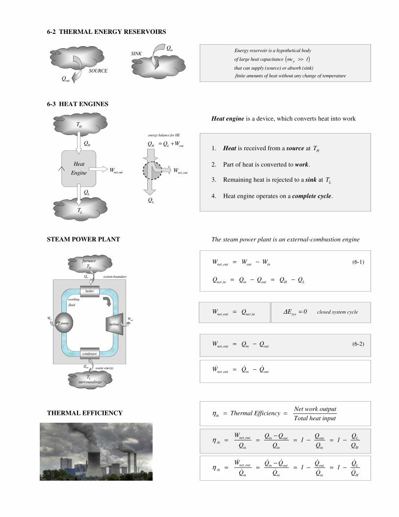
6-2 THERMAL ENERGY RESERVOIRS
6-3 HEAT ENGINES
Heat engine is a device, which converts heat into work
1. Heat is received from a source at H
T
2. Part of heat is converted to work. 3. Remaining heat is rejected to a sink at
LT
4. Heat engine operates on a complete cycle. STEAM POWER PLANT The steam power plant is an external-combustion engine
net ,out out inW W W= − (6-1)
net ,in in out H LQ Q Q Q Q= − = −
net ,out net ,inW Q =
sysE 0∆ = closed system cycle
net ,out in outW Q Q= − (6-2)
net ,out in out
W Q Q= −� ��
THERMAL EFFICIENCY th
Net work output Thermal Efficiency
Total heat inputη = =
net ,out
th
in
W
Qη = in out out L
in in H
Q Q Q Q 1 1
Q Q Q
−= = − = −
net ,out
th
in
W
Qη =
�
� in out out L
in in H
Q Q Q Q 1 1
Q Q Q
−= = − = −� � � �
� � �
outQ
SOURCE
SINKin
Q
( )p
Energy reservoir is a hypothetical body
of large heat capacitance mc 1
that can supply (source) or absorb (sink)
finite amounts of heat without any change of temperature
>>
turbine
boiler
condensor
pump
inQ
outW
outQ
inW
H
T
LT
furnace
surroundings
working
fluid
system boundary
waste energy
H L outQ Q W= +
LQ
net ,outW
L
T
H
T
Heat
Engine net,outW
HQ
LQ
energy balance for HE

THE SECOND LAW OF THERMODYNAMICS
Kelvin – Planck Statement: It is impossible for any device that operates on a cycle
to receive heat from a single reservoir and
produce a net amount of work
For heat engine to operate, the working fluid has
to exchange heat with heat sink as well with the heat source.
If L
Q 0= , then L th
H
Q1 1
Qη = − = , therefore, the 2nd Law claims that
no heat engine can be 100% efficient:
Clausius Statement: No device can operate on a cycle and produce effect
that is solely the heat transfer from
a lower-temperature body to a higher-temperature body
There are devices that can transfer heat
from lower-temperature reservoirs to higher-temperature reservoirs
but they have also to consume some energy Win
Equivalence of two statements:
If some device
violates one statement,
it also violates
the other statement,
and vice versa.
H
T
Heat
Engine net,outW
HQ
th < 1η
2) Attach heat engine to refrigerator 3) Violation of Clausius statement1) Assume that Kelvin-Planck statement is violated
L
T
H
T
H outQ =W
HQ
th
Heat
Engine
1η =
L
T
H
T
H LQ Q+
LQ
H inQ =W
HQ
th
Heat
Engine
1η =
Refrigerator
L
T
H
T
LQ
LQ
combine in a single device
Lord Kelvin
(1824-1907)
Max Planck
(1858-1947)
Rudolf Clausius
(1822-1888)
nd
Violation
of the 2 Law:
nd
Violation
of the 2 Law:
L
T
H
T
HQ
LQ

6-4 REFRIGERATOR Refrigerator transfers heat Objective: remove heat from a refrigeration space
from a low-temperature medium to a higher temperature medium
L L
R
Hin H L
L
Q Q 1COP = = =
QW Q Q1
Q
−−
L L
R
in H L H
L
Q Q 1COP = = =
W Q Q Q1
Q
−−
� �
� � � �
�
HEAT PUMP Heat pump transfers heat Objective: supply heat to a living space
from a low-temperature medium to a higher temperature medium
H H
HP
Lin H L
H
Q Q 1COP = = =
QW Q Q1
Q
−−
H H
HP
in H L L
H
Q Q 1COP = = =
W Q Q Q1
Q
−−
� �
� � � �
�
COEFFICIENT OF PERFORMANCE
6-5 PERPETUAL–MOTION MACHINES
PMM1 violates the 1st law of thermodynamics
PMM2 violates the 2nd law of thermodynamic
H L inQ Q W= +
LQ
inW
Q
LQ
inW
H L inQ Q W= +
compressor
condensor
evaporator
throttle
HQ
inW
LQ
HT
living space
LT
cold reservoir
Desired
Output
Vapor-compression
refrigeration
cycle
Desired outputCOP =
Required input
compressor
condensor
evaporator
throttle
HQ
inW
LQ
HT
LT
surroundings
refregerated space
working
fluid
refrigerant
=
Desired
Output
Vapor-compression
refrigeration
cycle
working
fluid
refrigerant
=
HEAT

Planck, p.86
§112. A process which can in no way be completely reversed is termed irreversible, all other processes reversible. That a process may be irreversible, it is not sufficient that it cannot be directly reversed. This is the case with many mechanical processes which are not irreversible (cf. 113). The full requirement is, that it be impossible, even with the assistance of all agents in nature, to restore everywhere the exact initial state when the process has once taken place. The propositions of the three preceding paragraphs, therefore, declare, that the generation of heat by friction, the expansion of a gas without the performance of external work and the absorption of external heat, the conduction of heat, etc., are irreversible processes. §115. Since there exists in nature no process entirely free from friction or heat-conduction, all processes which actually take place in nature, if the second law be correct, are in reality irreversible ; reversible processes form only an ideal limiting case. §116. The second fundamental principle of thermodynamics being, like the first, an empirical law, we can speak of its proof only in so far as its total purport may be deduced from a single self-evident proposition.
We, therefore, put forward the following proposition as being given directly by experience : It is impossible to construct an engine which will work in a complete cycle, and produce no effect except the raising of a weight and the cooling of a heat-reservoir. Such an engine could be used simultaneously as a motor and a refrigerator without any waste of energy or material, and would in any case be the most profitable engine ever made. It would, it is true, not be equivalent to perpetual motion, for it does not produce work from nothing, but from the heat, which it draws from the reservoir. It would not, therefore, like perpetual motion, contradict the principle of energy, but would, nevertheless, possess for man the essential advantage of perpetual motion, the supply of work without cost ; for the inexhaustible supply of heat in the earth, in the atmosphere, and in the sea, would, like the oxygen of the atmosphere, be at everybody's immediate disposal.

6-7 THE CARNOT CYCLE
6-8 CARNOT PRINCIPLES Efficiency of two Heat Engines operating between the same two reservoirs at L
T and H
T
C1
irreversible reversible η η<
C2 reversible 1 reversible 2
η η=
6-9 THE THERMODYNAMIC TEMPERATURE SCALE For reversible heat engine operating between L
T and H
T :
L L
H H
Q T
Q T= Kelvin Scale of Absolute Temperature
6-10 THE CARNOT HEAT ENGINE The efficiency of heat engine operating on a reversible Carnot cycle between L
T and H
T :
L L
C
H H
Q T 1 1
Q Tη = − = −
6-11 THE CARNOT HEAT PUMP Carnot Heat Pump: Carnot Refrigerator:
CHP
L L
H H
1 1COP
Q T1 1
Q T
= =
− −
CR
H H
L L
1 1COP
Q T1 1
Q T
= =
− −
H
H
Isothermal expansion
at T
heat Q is added
3
2
insulated
1
4
insulated
4
3
LQ
L
L
Isothermal compression
at T
heat Q is rejectedL
Adiabatic expansion
Q=0
Temperature dropped to TH
Adiabatic compression
Q=0
Temperature raised to T
The Carnot Cycle consists
of 4 reversible processes
IR
IR Rη η<
HT
LT
R1 R2
R1 R2η η=
(Refrigerator, Heat Pump)The Reversed Carnot Cycle
P
HT
V
net ,outW
1V
1
2
3
4
4V
2V
3V
LT
P
HT
V
net ,inW
1V
1
2
3
4
2V
4V
3V
LT
(Heat Engine)The Carnot Cycle
HQ
LQ
LT
HT
HQ
LQ
LT
HT
C
L H
is the highest possible efficiency
of the heat engine operating between
two reservoirs at T and T
η
gas
continues
to expand
gas
1V
2V
2V
3V
3V
4V
4V
1V
nd
Violation of Carnot Principles
yields violation of the
2 Law of Thermodynamics
Carnot
Efficiency
Reversible Processes
1
2
HQ
Q 0=Q 0= Q 0=Q 0=
the paths coinside•
at thermal equilibrium•
heat transfer is due to infinitely
small difference in temperature
•
1
2
Q1
2
-Q
-W W
Sadi Carnot (1822-1888)
Irreversible Processes
heat transfer is due to finite
difference in temperature
•
T 0∆ >
heat generation by friction•

INSTITUT NATIONAL DES SCIENCES APPLIQUEES, LYON

In statistical thermodynamics
entropy is treated as a measure
of molecular disorder
2nd
LAW OF THERMODYNAMICS – ramification
Q
0T
δ≤∫�
rev
Q0
T
δ =
∫�
7-1 ENTROPY Clausius: “I propose to name the quantity S the entropy of the system, after the Greek word τροπη [trope], the transformation”
dS rev
Q
T
δ =
definition of the differential of entropy
S∆ 2 1
S S= − 2
rev1
Q
T
δ =
∫ change of entropy during rev. process
S kJ
K
total entropy
S
sm
= kJ
kg K
⋅ specific entropy (entropy)
7-2 ENTROPY CHANGE AND ENTROPY GENERATION
Q
T
δ∫�
2
1
Q
T
δ= ∫
1
rev2
Q
T
δ +
∫
2
1
Q
T
δ= ∫
1
2
dS+ ∫ 0≤
2
1
Q
T
δ∫ 1 2
S S+ − 0≤
2 1
S S− 2
1
Q
T
δ≥ ∫
INCREASE OF ENTROPY PRINCIPLE
2 1
S S− 2
gen
1
Q S
T
δ= +∫
genS 0≥
isolated
S 0∆ > ( )isolated revS 0∆ =
Clausius Inequality
Carnot
Cycle
impossible
The Universe is Entropy (disorder)
an isolated of the Universe
system is increasing
⇒
gen
Entropy change S
can be negative,
but entropy generation
S cannot:
∆
( )
Entropy of irreversible
isolated system Q 0
is
during a process
=
increasing
entropy transfer with heat entropy generationentropy change
for all
cycles
for any
reversible
cycle
entropy is an extansive property:
1 2 3S S S S∆ ∆ ∆ ∆= + +
1S∆
2S∆
3S∆
T
reversible process
S
= ∫2
1
Q TdS
1S
2S
T
reversible process
dSS
Q TdSδ =
1S
2S
T
Kelvin-Planck Clausius
2 4
H L L H L
Carnot H L L L H1 3
Q Q Q Q TQ Q Q 1 0
T T T T T T Q T
δ δ δ = + = − = − =
∫ ∫ ∫�
HT
Q
LT
W
HT
Q
LT
Q
impossible
( )7-9 ( )7-11
( )7-7
( )7-10
( )7-4
Arbitrary process
Reversible1
2
lnS k p=

7-5 T-S DIAGRAM
Internally reversible process dS int rev
Q
T
δ =
( )7-4 ⇒ Qδ TdS= ( )7-14
Q 2
1
TdS= ∫ ( )7-15
q 2
1
Tds= ∫ ( )7-17
Isothermal Process
Q ( )0 2 1T S S= ⋅ − ( )7-18
q ( )0 2 1T s s= ⋅ − ( )7-19
7-4 Isentropic process ( S const= )
Example 7-6 Carnot Cycle
net ,inQ
net ,out W=
net ,out
W H L
Q Q= −
h-s diagram (Mollier diagram, p.345) is useful for analysis of steady-flow devices
T
S
Area Q=
1S
2S
1
2
Internally
reversible
process
Heat transfer during
the internally
reversible process
reversible adiabatic
isentropic process
�
isentropic process
is associated with
internally reversible
adiabatic process
w h∆=For adiabatic steady-flow devices:
nozzles, turbines, compressors, etc.
Richard Mollier (1863 1935)−
For internally
reversible process
T
S
Q 0=
1 2S S=
1
2
T
S
net ,out H LW Q Q= −
1 4S S=
2 3S S=
1 2
HT
4 3L
T
HQ
LQ
T
S
Q
1S
2S
1 2
isothermal
process is
internally
reversible0
T
q T s∆= For isothermal processes
h
s
s∆
1s
2s
1
2
h∆measure
of work
output
measure of the
irreversibilities
1h
2h

7-7 GIBBS EQUATIONS – THE Tds RELATIONS
W PdVδ = boundary work
Q Wδ δ− dU= Q TdSδ = for reversible process
⇓
TdS dU PdV= +
Tds du Pdv= +
ds 1 P
du dvT T
= +
Tds dh vdP= −
ds 1 v
dh dPT T
= −
ENTROPY CHANGE ISENTROPIC PROCESS, ∆S=0
7-8 LIQUIDS AND SOLIDS v p
c c c= = , dv 0= (incompressible substance)
ds 1
du T
=dT
c T
=
2 1
s s− 2
avg
1
T c ln
T=
2 1T T=
7-9 IDEAL GAS Pv RT= , v
du c dT= , p
dh c dT= Isentropic process
ds v
dT dv c R
T v= + 1st Gibbs Eq
ds p
dT dP c R
T P= − 2nd Gibbs Eq
Constant specific heats: v ,avgc , p,avg
c at 1 2
avg
T TT
2
+=
2 1
s s− 2 2
v ,avg
1 1
T v c ln R ln
T v= + ( )7-33
k 1
2 1
1 2
T v
T v
−
=
2 1
s s− 2 2
p ,avg
1 1
T P c ln R ln
T P= − ( )7-34
k 1
k2 2
1 1
T P
T P
−
=
k
2 1
1 2
P v
P v
=
2 1
s s− o o 2
2 1
1
P s s R ln
P= − − ( )7-39 o 0 2
2 1
1
Ps s R ln
P= +
( )T
o
p
0
dTs c T
T= ∫ , ( )
2
o o
2 1 p
1
dTs s c T
T− = ∫ 2 r 2
1 r1
P P
P P= 2 r 2
1 r1
v v
v v=
Start with closed system
energy balance
for reversible process
Gibbs equations do not depend
on the type of the process
(reversible and irreversible),
they are valid both for
closed and open systems (p.350),
because they include only properties
where, the temperature dependent part of entropy is defined by:
( )1 2 s s is an isothermal process :=Isentropic process
Isentropic process
( )1 2 s s=Isentropic process
( )−=
1 k kTP C
( )7 49− ( )7 50−
o
r r s ,P ,v
Table A-17
( )7-25st1 Gibbs Equation
( )7-26nd2 Gibbs Equation
= −p vR c c
=p
v
ck
c
= −v
Rk 1
c
Exact Analysis
Table A-2
Specific
heat ratio−
=k 1
Tv C
=k
Pv C
relative specific pressure and volume:
T
ss∆1
s2
s
1
2
1T
2T
1P
2P
v
1c R
k 1=
−
p
kc R
k 1=
−
=(polytropic process with n k )
T
s
1 2s s=
1
2
1T
2T
1P
2P
h u Pv
dh du Pdv vdP
= +
= + +
u h Pv
du dh Pdv vdP
= −
= − −
(1839-1903)
( )7-38

7-10 REVERSIBLE STEADY-FLOW WORK
rev revq w dh dke dpeδ δ− = + + Energy balance
revq Tds dh vdPδ = = − nd
2 Gibbs equation
rev
w vdP dke dpeδ = − − −
2
rev ,net ,out
1
w vdP ke pe∆ ∆= − − −∫ ( )7-51
= − ∫2
rev ,out
1
w vdP ( )7-52 turbine
= ∫2
rev ,in
1
w vdP compressor
rev ,out act ,outw w≥
rev ,in act ,inw w≤
7-11 Compression work for ideal gas (p.364)
( )
k 1
k1 2
comp ,in 2 1
1
kRT Pkw R T T 1
k 1 k 1 P
− = − = − − −
( )
n 1
n1 2
comp ,in 2 1
1
nRT Pnw R T T 1
n 1 n 1 P
− = − = − − −
2
comp,in
1
Pw RT ln
P=
Incompressible fluid ( v const= , 7-51) ⇒ ( )rev 2 1w v P P ke pe∆ ∆= − − − − ( )7-54
Bernoulli equation (steady flow of incompressible fluid through the simple pipe without friction)
( )2 2
2 1 2 1
2 1
P P V Vg z z 0
2ρ
− −+ + ⋅ − = ( )7-55
( )
Danila Bernoulov
1700 1782−
�
act act
rev rev
act rev act rev
rev act rev act
Tds
rev act act
gen
q w dh dke dpe
q w dh dke dpe
q q w w 0
w w q q
w w qds s 0
T T
δ δ
δ δ
δ δ δ δ
δ δ δ δ
δ δ δ
− = + +
− = + +
− − + =
− = −
−= − = ≥
pipe
inlet state
w 0=
outlet state
1 2
qδinlet state
wδ
outlet state
1 2
k
Isentropic process
Pv const=
Isothermal process
Pv const=
n
Polytropic process
Pv const=
−
=
1
kv cP
−
=
1
nv cP
1v cP
−=
P
v
1P
2P
( )isothermal n 1=
( )polytropic 1 n k< <
( )isentropic n k=
Flow through the pipe which involves no work interaction
Pv RT=Ideal gas
Reversible work output for
steady-flow and closed systems
( )for ke pe 0∆ ∆= =
Equations 7-57 a,b,c
outQ maximum
heat transfer
Q 0=
T const=
rev ,out act ,outw w≥
reversible
actual
turbine
compression
P
v1
v2
v
1
2
1P
2P
turbine
in derivation, we assume that both
processes are between the same states
turbine
compression
Steady-flow devices
deliver the most and
consume the least work
when the process is
reversible
≥rev ,net ,out act ,net ,out
w w
δ δ≥rev act
w w
Eq.7-9
minimum
heat transfercomp ,in
w
By cooling compressor, the requiered work input
can be minimized to achive the same pressure increase
temperature
is increased
P
v1
v2
v
1
2
1P
2P
rev ,outw
turbine

ISENTROPIC EFFICIENCIES η is a measure of the deviation of actual process from the corresponding isentropic process
Turbine
aT
s
wactual work
isentropic work wη = =
1 2aT
1 2s
h h
h hη −
=−
Compressor and pump
sC
a
wisentropic work
actual work wη = =
2s 1C
2a 1
h h
h hη −
=−
compressor
( )2 1
P2a 1
v P P
h hη
−=
− pump
Nozzle
= =2
2aN 2
2s
Vactual KE at exit
isentropic KE at exit Vη
2
2a1 2a
Vh h
2= +
1 2aN
1 2s
h h
h hη −
=−
h
s
1
1P
2P
isentropic
actual
1h
2ah
2sh
aw sw
h
s
1
2P
1P
isentropic
actual
1h
2ah
2sh
aw sw
h
s
1
1P
2P
isentropic
actual
1h
2ah
2sh
aw sw
s2
s2
s2
a2
a2
a2
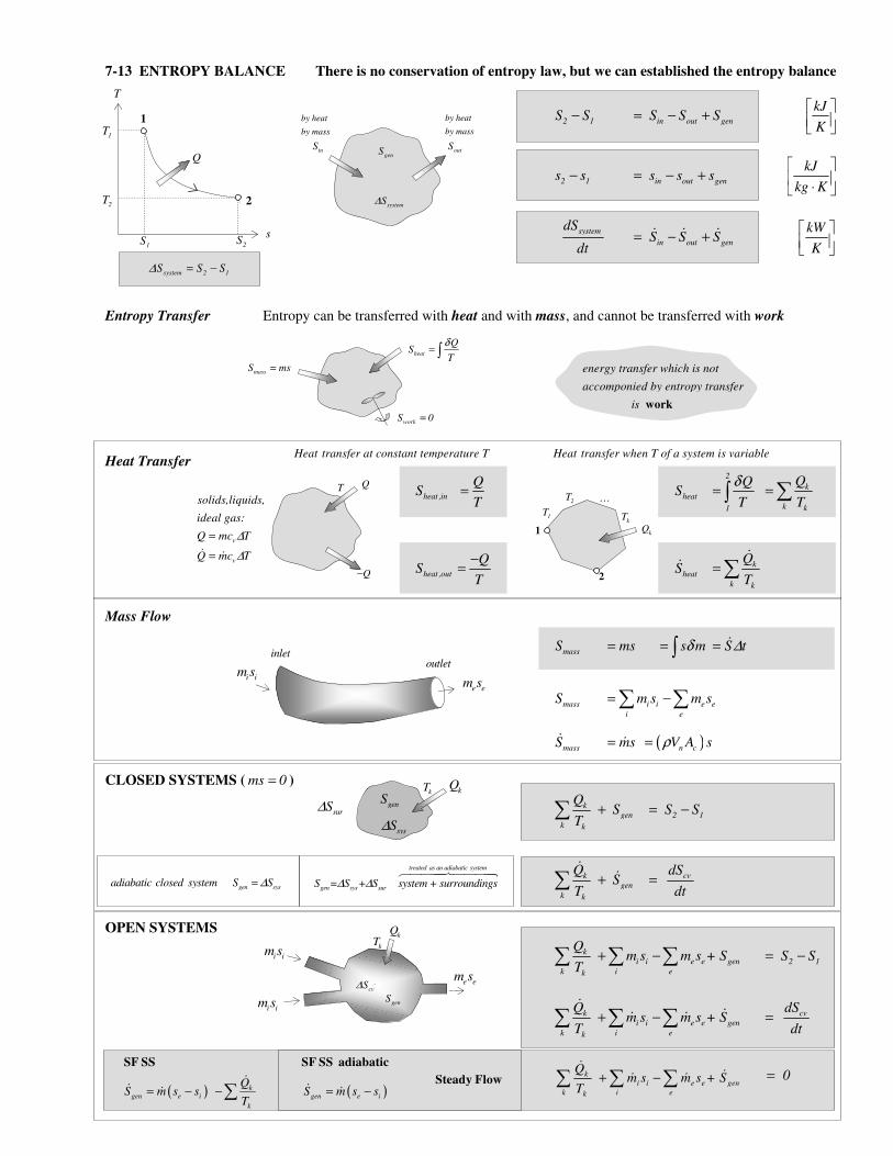
7-13 ENTROPY BALANCE There is no conservation of entropy law, but we can established the entropy balance
2 1
S S− in out gen
S S S= − + kJ
K
2 1
s s− in out gen
s s s= − + kJ
kg K
⋅
system
dS
dt
in out gen S S S= − +� � �
kW
K
Entropy Transfer Entropy can be transferred with heat and with mass, and cannot be transferred with work Heat Transfer
heat ,in
S Q
T=
heatS
2
1
Q
T
δ= ∫ k
k k
Q
T=∑
heat ,out
SQ
T
−=
heatS� k
k k
Q
T=∑
�
Mass Flow
mass
S ms= s mδ= ∫ S t∆= �
mass
S i i e e
i e
m s m s= −∑ ∑
mass
S� ms= � ( )n cV A sρ=
CLOSED SYSTEMS ( ms 0= )
k
gen
k k
Q S
T+∑
2 1 S S= −
k
gen
k k
Q S
T+∑
�� cv
dS
dt=
OPEN SYSTEMS
k
i i e e gen
k i ek
Q m s m s + S
T+ −∑ ∑ ∑
2 1 S S= −
k
i i e e gen
k i ek
Q m s m s + S
T+ −∑ ∑ ∑
��� � cv
dS
dt=
kQ
kT
inlet
i im s
outlet
e em s
v
v
solids,liquids,
ideal gas:
Q mc T
Q mc T
∆
∆
=
=� �
1T
2T �
energy transfer which is not
accomponied by entropy transfer
is work
workS 0=
heat
QS
T
δ= ∫
massS ms=
surS∆
genSin
S
systemS∆
outS
by heat
by mass
by heat
by mass
vm,c
( ) ( )k
gen e i gen e i
k
QS m s s S m s s
T= − − = −∑
SF SS SF SS adiabatic
�� �� �
T Q
Q−
genS
kQ
i im s
kQ
cvS∆
kT
e em s
genS
i im s
kT
sysS∆
treated as an adiabatic system
gen sys surS = S + S system + surroundings ∆ ∆
�����������
gen sysadiabatic closed system S S∆=
T
s
system 2 1S S S∆ = −
1S 2
S
1
2
1T
2T
Q
Heat transfer at constant temperature T Heat transfer when T of a system is variable
1
2
Steady Flowk
i i e e gen
k i ek
Q m s m s + S
T+ −∑ ∑ ∑
��� � 0=

9-1 GAS POWER CYCLES – BASICS Power cycles (heat engines) produce work from heat.
Thermal efficiency: net net
th
in in
W w
Q qη = = L
th Carnot
H
T 1
Tη η≤ = −
Ideal power cycle: ● all processes are internally reversible
● no friction
● quasi-equilibrium expansion and compression
● no heat loss between devices
● negligible change in KE and PE
Air-standard cycle: ● working fluid is air (ideal gas)
● all processes are internally reversible
● combustion process is modeled by heat transfer H
Q from reservoir at H
T
● exhaust process is modeled by heat transfer L
Q to reservoir at L
T
● cold air assumption: v
c 0.718= , p
c 1.005= kJ
kg K
⋅ , k 1.4= , R 0.287=
Ideal air-standard cycle (internally reversible) is not, in general, a Carnot cycle (totally reversible)
9-2 CARNOT CYCLE ( )H H 2 1Q T S S= − ( )H H 2 1
q T s s= −
( )L L 3 4Q T S S= − ( ) ( )L L 3 4 L 2 1
q T s s T s s= − = −
Kelvin scale
H L L L
Carnot
H H H
Q Q Q T1 1
Q Q Tη
−= = − = −
( )
( )L 2 1L L L
Carnot
H H H 2 1 H
T s sQ q T1 1 1 1
Q q T s s Tη
−= − = − = − = −
−
( ) ( ) ( )L
net ,out Carnot H H 2 1 H L 2 1
H
Tw q 1 T s s T T s s
Tη
= ⋅ = − ⋅ ⋅ − = − ⋅ −
9-4 RECIPROCATING ENGINE (piston-cylinder device)
HT
T
S
net ,in H L net ,outQ Q Q W= − =
1 4S S=
2 3S S=
1 2
HT
4 3L
T
HQ
HT
LQ
net ,outW
actual
cycle
ideal
cycle HT
LT
LQ
HQ
net ,outW
( )Spark ignition engines SI
Internal combustion engines
Displacement volumemax min
V V−
Compression ratio
BDC max max
TDC min min
V V vr
V V v= = =
Mean Effective Pressure
net net
max min max min
W wMEP
V V v v= =
− −
net net
minmaxmax
max
w wMEP
1vv 1v 1
rv
= =
−−
( )net net
minmax
min
min
w wMEP
v r 1vv 1
v
= =−
−
( )Compression ignition engines CI
TDS
top dead center
bore
BDS
bottom dead center
stroke
clearance
volume
displacement
volume
MEP
P
minVmaxV
V
( )net max minW MEP V V= ⋅ −
netW
mean
effective
pressure

RECIPROCATING ENGINES – OVERVIEW
SI spark-ignition engines (combustion is initiated by a spark plug) CI compression-ignition engines (combustion is self-ignited as a result of compression)
( )Spark ignition engines SI
TDS
top
dead
center
bore
BDS
bottom
dead
center
stroke
clearance
volume
displacement
volume
MEP
P
minVmaxV
V
( )net max minW MEP V V= ⋅ −
netW
mean
effective
pressure
Internal combustion engines
Reciprocating engine (piston-cylinder device)
Displacement volumemax min
V V−
Compression ratio BDC max max
TDC min min
V V vr
V V v= = =
Mean Effective Pressure net net
max min max min
W wMEP
V V v v= =
− −
net net
minmaxmax
max
w wMEP
1vv 1v 1
rv
= =
−−
( )net net
minmax
min
min
w wMEP
v r 1vv 1
v
= =−
−
( )Compression ignition engines CI

9-5 OTTO CYCLE – SPARK-IGNITION ENGINES
Actual 4-stroke spark-ignition engine Ideal Otto cycle (air-standard cycle)
( ) ( )in out out inq q w w u∆− − − =
cycle
0= ⇒ net ,out in out
w q q= −
:→2 3 ( )in 3 2 v 3 2q u u c T T= − = −
:→4 1 ( )out 4 1 v 4 1q u u c T T= − = −
k 1k 1
1 2 3 4
k 1
2 1 4 3
T v 1 v T
T v r v T
−−
−
= = = =
⇒ 3 4
2 1
T T
T T=
k
k2 1
1 2
P vr
P v
= =
th ,Otto
η net out 4 1
in in 3 2
w q T T 1 1
q q T T
−= = − = −
−
4
11
2 3
2
T1
TT 1
T T1
T
−
= −
−
k 1
1 2
2 1
T v 1 1
T v
−
= − = −
k 11
1r
−
= −
1 k
1 r−
= −
( )Energy balance Otto cycle is executed in a closed system :
isentropic
compression
heat
addition
v const=
isentropic
expansion
heat
rejection
v const=
P
V
1
2
4
3
′4
compression
ignition
expansion
exhaust
intake
( )2 3 4 1Isentropic processes 1-2 and 3-4 with v v and v v := = under cold air assumption
( )heat transfer at v const w 0= =
( )Thermal efficiency of the ideal Otto cycle :under cold air assumption
Nikolaus Otto
(1832-1891)
Beau de Rochas
(1815-1893)http : // www.keveney.com / Engines.html
thermal efficiency
of Otto cycle under
cold air assumption
T
1 2s s=s
1
2 4
3
inq
outq
2 3 maxv v v= =
1 4 minv v v= =
3 4s s=
isentropic
expansion
isentropic
compression
p
v
ck
c=
Typical
compression
ratios for
gasoline
engines
argon
helium
air
2CO
actual engines
thermal efficiency
of Otto cycle under
cold air assumption:
1 k1 rη −
= −
compression
ratio41
2 3
vvr
v v= =
P
2 3v v= 1 4v v=
V
1
2 4
3
inq
outq
isentropic
expansion
isentropic
compression
ignition
compression
11
2 2 3
4 4
′4 ′4
( )
expansion
power
ignition
exhaust intake
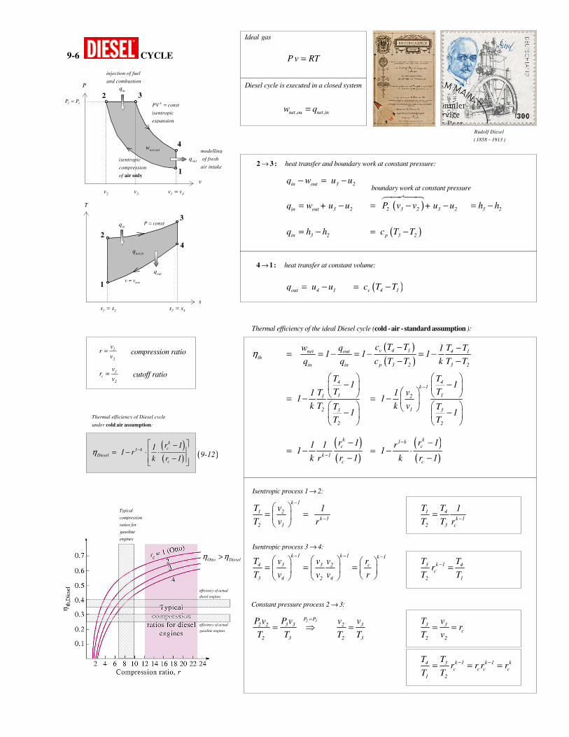
9-6 CYCLE
in out 3 2q w u u− = −
in out 3 2
q w + u u = − ( )2 3 2 3 2 P v v + u u= − −
�����
3 2
h h = −
= −in 3 2
q h h ( )p 3 2 c T T= −
= −out 4 1
q u u ( )= −v 4 1 c T T
th
η ( )
( )v 4 1net out 4 1
in in p 3 2 3 2
c T Tw q T T1 1 1 1
q q c T T k T T
− −= = − = − = −
− −
4
11
2 3
2
T1
TT1 1
k T T1
T
−
= −
−
4k 1
12
1 3
2
T1
Tv1 1
k v T1
T
−
−
= −
−
( )( )
k
c
k 1
c
r 11 1 1
k r 1r−
−= −
−
( )( )
k1 kc
c
r 1r 1
k r 1
− −= − ⋅
−
k 1
1 2
k 1
2 1
T v 1
T v r
−
−
= =
41
k 1
2 3 c
TT 1
T T r−
=
k 1 k 1 k 1
4 3 3 c2
3 4 2 4
T v v rv
T v v v r
− − −
= = =
k 13 4
c
2 1
T Tr
T T
−=
3 32 2
2 3
P vP v
T T=
2 3P P=
⇒ 32
2 3
vv
T T= 3 3
c
2 2
T vr
T v= =
k 1 k 1 k4 3
c c c c
1 2
T Tr r r r
T T
− −= = =
T
1 2s s=s
1
2
4
3
inq
outq
P const=
minv v=
3 4s s=
Diesel cycle is executed in a closed system
Thermal efficiency of the ideal Diesel cycle ( ):cold -air - standard assumption
compression ratio1
2
vr
v=
3
c
2
vr
v= cutoff ratio
( )( )
k
c1 k
Diesel
c
r 11 1 r
k r 1η −
− = − ⋅ ⋅
−
Thermal efficiency of Diesel cycle
under :cold air assumption
Typical
compression
ratios for
gasoline
engines
efficiency of actual
diesel engines
efficiency of actual
gasoline engines
Otto Dieselη η>
heat transfer and boundary work at constant pressure:→2 3 :
heat transfer at constant volume:→4 1:
( )9-12
Isentropic process 1 2:→
Ideal gas
boundary work at constant pressure
Isentropic process 3 4:→
P
2v 1 4v v=
v
1
2
4
3inq
outq
kPV const
isentropic
expansion
=
isentropic
compression
of air only
2 3P P=
injection of fuel
and combustion
3v
modelling
of fresh
air intake
net,outw
net,inq
net ,ou net ,inw q=
Rudolf Diesel
( 1858 1913 )−
Constant pressure process 2 3:→
P v RT=

STIRLING CYCLE https://www.stirlingengine.com/
ERICSSON CYCLE
External combustion engine
( )
Reverend Robert Stirling
1790 1878 −
( )
John Ericsson
1803 1889 −
External combustion engine
T
4vs
1
2
4
3
inqoutq
2v
P
4s 3sv
1 2
4 3
inq
outq
P=const
HT
1s
regeneratorP=const
2s
regenerator
LT
T
1 4v v=s
1
2
4
3
inq
outq
HT const=
2 3v v=
P
4s 3sv
1 2
4 3
inq
outq
v=const
HT
1s
regeneratorv=const
2s
regenerator
LT const=
LT
L
th
H
T 1
Tη = −
Carnot
Thermal efficiency of Stirling cycles
Ericsson
-9 7

9-8 BRAYTON CYCLE
( )in 3 2 p 3 2q h h c T T= − = − ( )comp,in 2 1 p 2 1
w h h c T T= − = −
( )out 4 1 p 4 1q h h c T T= − = − ( )turb,out 3 4 p 3 4w h h c T T= − = −
net ,out in outw q q= −
3 2 4 1h h h h= − − +
( )3 4 2 1h h h h= − − −
turb ,out comp ,inw w= −
k 1k 1k 1 kk
3 32 2 kP
1 1 4 4
P TT Pr
T P P T
−−−
= = = =
32P
1 4
PPr
P P= = pressure ratio
4 3
1 2
T T
T T=
B
η net ,out
in
w
q= out
in
q1
q= − 4 1
3 2
T T1
T T
−= −
−
4
1
1 1
23
2
2
TT 1
T T1 1
TTT 1
T
−
= − = −
−
B
η k 1
kP
11
r
−= −
P
2v4v
v
1
2
4
3inq
outq
P const=
1v
s const=s const=
Gas-Turbine Engines
Open Cycle Closed Cycle
For isentropic processes 1-2 and 3-4:
( )Thermal efficiency of Brayton cycle :under cold -air assumption
( )
George Brayton
1830 1892−
⇓
T
1 2s s=s
1
2
4
3
inq
outq
P const=
P const=
3 4s s=
maxT
minT
The Ideal Bryton Cycle:
Steady-Flow

10-2 RANKINE CYCLE
turbinepump
inq
outw
outq
inw
boiler
condensor
1
2
4
3
Vapor power cycles working fluid is alternately vaporized and condensed−
1 2 Pump:→in 2 1w h h= − ( )in 1 2 1w v P P= −
11 f @Pv v=11 f @Ph h=
2 3 Boiler:→in 3 2q h h= −
3 4 Turbine:→out 4 3w h h− = −
4 1 Condenser:→out 1 4q h h− = −
2 1 inh h w= +
( )
net ,outnet ,inwq
in out out inq q w w 0− − − =
����������
Energy balance for a single stream steady-flow devices:
incompressible fluid
Ideal Rankine sycle:
T
s
inw
1 2s s=
= =2 3P P const
1
2
4
3inq
outq
3 4s s=
outw
= =1 4P P const
net out 4 1
th
in in 3 2
w q h h 1 1
q q h hη
−= = − = −
−
1 BtuHeat rate
kWh=
[ ]Amount of heat supplied in Btu
to generate 1 kWh of electricity
( )1820 1872−
Energy balance for a cycle:
Coefficient of thermal
efficiency used in US
[ ]
[ ]th
3412 Btu kWh
Heat rate Btu kWhη =

11 REFRIGERATION CYCLES
L L
R
Hin H L
L
q q 1COP = = =
qw q q1
q
−−
H H
HP
Lin H L
H
q q 1COP = = =
qw q q1
q
−−
11-2 REVERSED CARNOT CYCLE
L
R,Carnot
H Hin
L L
q 1 1COP = = =
q Tw1 1
q T− −
H
HP,Carnot
L Lin
H H
q 1 1COP = = =
q Tw1 1
q T− −
11-3 IDEAL REFRIGERATION CYCLE
1 4L
R
net,in 2 1
h hqCOP = =
w h h
−
−
2 3H
HP
net,in 2 1
h hqCOP = =
w h h
−
−
Refrigeration heat transfer from a lower temperature region to a higher temperature region−
Vapor-compression refrigeration cycle working fluid (refrigerant) is
vaporised and condensed alternately and is compressed in the vapor phase
−
H L inQ Q W= +
LQ
inW
objective:
remove heat from a refrigeration space:
−Refrigerator
objective:
supply heat to a living space:
−Heat pump
T
s
inw
s3 4s s=
P const=
1
2
4
3
L inq q=
outq
1 2s s=
P const=
s4
4s
1 2 Compressor:→in 2 1w h h= −
2 3 Condenser:→ out 2 3q h h= −
3 4 Throttle:→ 3 4h h=
4 1 Evaporator:→in 1 4q h h= −
P
h
in 2 1w h h= −
3 4h h=
1
2
4
3
in 1 4q h h= −
out 2 3q h h= −
1h 2h
T
s
inw
3 4s s=
P const=
1
2
4
3
LQ
HQ
1 2s s=
P const=
( ) ( )in out out in e iq q w w h h− − − = −SF SS
1
2
4
3
compressor
condensor
evaporator
throttle
Hq
inw
Lq
HT
LT
working
fluid refrigerant=
Vapor-compression
refrigeration
cycle
4
Top Related