


Languages
Pages
Legal


Munich Personal RePEc Archive
Beliefs and (In)Stability in Normal-FormGames
Hyndman, Kyle and Terracol, Antoine and Vaksmann,
Jonathan
23 May 2013
Online at https://mpra.ub.uni-muenchen.de/47221/
MPRA Paper No. 47221, posted 27 May 2013 13:31 UTC

Beliefs and (In)Stability in Normal-Form Games
Kyle HyndmanMaastricht University, [email protected], http://www.personeel.unimaas.nl/k-hyndman
Antoine TerracolParis School of Economics & Centre d’Economie de la Sorbonne, Universite Paris 1 - Pantheon Sorbonne, CNRS,
[email protected] Corresponding author
Jonathan VaksmannGAINS-TEPP, Universite du Maine & Centre d’Economie de la Sorbonne, Universite Paris 1 - Pantheon Sorbonne, CNRS,
In this paper, we use experimental data to study players’ stability in normal-form games where subjects
have to report beliefs and to choose actions. Subjects saw each of 12 games four times in a regular or
isomorphic form spread over two days without feedback. We document a high degree of stability within the
same (strategically equivalent) game, although time and changes in the presentation of the game do lead
to less stability. To look at stability across different games, we adopt the level−k theory, and show that
stability of both beliefs and actions is significantly lower. Finally, we estimate a structural model in which
players either apply a consistent level of reasoning across strategically different games, or reasoning levels
change from game to game. Our results show that approximately 30% of subjects apply a consistent level
of reasoning across the 12 games, but that they assign a low level of sophistication to their opponent. The
remaining 70% apply different levels of reasoning to different games.
Key words : Game theory, Beliefs, Stability, Level-k thinking, Experiment
JEL codes : C72, C91, D83
History : May 23, 2013
1. Introduction
When deciding on an action to take in normal-form games, players must form beliefs about the
action(s) that will be taken by their opponent(s). That is, they must have a theory of the mind of
their opponents. Several such theories have been proposed in the literature. In static, normal form
games, the benchmark is Nash reasoning, which assumes that players form beliefs and perfectly
best-respond to them. Moreover, in the equilibrium, beliefs and actions are self-reinforcing in the
sense that the observed action profile justifies the underlying beliefs (and vice-versa). However, in
many situations, behavior frequently deviates from the Nash benchmark. Because of this, other
approaches designed around boundedly rational or error prone decision makers have arisen. Notable
examples of those approaches are Quantal Response Equilibrium (McKelvey and Palfrey 1995);
Noisy Introspection (Goeree and Holt 2004); Level-k models (Nagel 1995, Stahl and Wilson 1994,
1

2 Hyndman, Terracol and Vaksmann: Beliefs and (In)Stability in Normal-Form Games
1995, Costa-Gomes et al. 2001) or Cognitive Hierarchy models (Camerer et al. 2004) in which
subjects vary according to their strategic reasoning or sophistication, with higher levels of reasoning
being represented as more iterations of best-response. There is a now extensive literature about
the ability of these models to rationalise observed behaviour in the lab; with Level-k and Cognitive
Hierarchy models appearing to be ahead in this horse race (see, e.g, Costa-Gomes and Crawford
2006, Costa-Gomes et al. 2009, Crawford et al. 2013).
Much less, however, is known about the stability of the belief formation process. Such a sta-
bility would be a very desirable feature as it would allow out of sample predictions and counter-
factual analysis. Lack of stability would mean that agents form beliefs and expectations in largely
unpredictable ways, thus rendering many economic policies less reliable due to the greater unpre-
dictability of behaviour. Several degrees of stability are worth looking at. The first, most basic, is
stability across identical situations. The second is stability across equivalent – but not identical
– strategic situations; and the last, most general and arguably most desirable, is stability across
different strategic situations. In this paper, we design an experiment that allows us to look at all
three degrees of stability, as well as the stability of subjects across time.
The experimental literature provides mixed evidence about the stability of strategic behaviour.
Coming out in favour of stability, Camerer et al. (2004) provide evidence that the distribution
of levels of reasoning is stable across games. Stahl and Wilson (1995) is an example of a paper,
like ours, that looks at stability of individual players’ level of reasoning across games and show
that many of their subjects possess a fair degree of stability. Their methodology, however, is likely
to overstate stability (Georganas et al. 2010). In contrast, several studies have shown much less
stability across games. Most recently, Georganas et al. (2010) show that stability of levels of
reasoning is moderate at best, and depends on the class of games being played. They also show
that one’s performance on quizzes designed to measure strategic reasoning and general intelligence
do not predict stability well.
These papers, however, have mostly used action data. In addition to the fact that actions may
not reflect underlying beliefs (Costa-Gomes and Weizsacker 2008), it has been argued (e.g. Manski
2002, 2004) that action data are, by themselves, insufficient to estimate decision rules, and that
information on beliefs is crucial. Our study uses both belief and action data, and thus allows for
a more direct investigation of the belief formation process. Moreover, these papers rely on specific
theories of the mind (mostly level-k), while we do so only for the third degree of stability.
Agranov et al. (2012) demonstrate that some players are unstable in the sense that they adjust
their strategy according to their beliefs about the level of strategic sophistication of their opponent.

Hyndman, Terracol and Vaksmann: Beliefs and (In)Stability in Normal-Form Games 3
This instability is triggered by changes in the information given to subjects about their opponent.
Similarly, Georganas et al. (2010) show that some players adjust their strategies when playing
against stronger opponents. In this paper, we investigate whether instability occurs without any
variation in the information about the opponent.
In our experiment, we chose 12 3× 3 normal-form games. For each game we had a “regular”
and “isomorphic” representation (obtained by adding or subtracting a constant and rearranging
the rows and/or columns). Subjects participated over two days, separated either by one day or
one week. On each day, they played 24 games, seeing each of the 12 games twice (though possibly
under a different frame). Subjects received no feedback until the end of the second day. Therefore,
over the two days, a given strategic structure is displayed four times to the subjects, either in its
regular or isomorphic versions. As the equilibrium structure of a given game is not affected by the
isomorphic transformation, these four instances represent a set of strategically equivalent games.
Therefore, we are able to study stability across several interesting dimensions. In particular,
we can compare stability both within and across sets of strategically equivalent games, and we
can also gain insights into whether the framing of the game or the time between instances of the
same game has an impact on stability. We also varied the characteristics of the games subjects
played; in particular, four games were dominance solvable games with one Nash equilibrium in
pure strategies, four games were not dominance solvable, but also had one Nash equilibrium in
pure strategies, and four games had two Nash equilibria in pure strategies. As stated above, one
other difference between our study and much of this literature is that we are interested in both the
stability of actions and the stability of underlying beliefs. Therefore, in our study, subjects chose an
action and stated beliefs about the likely action of their opponent. This allows us to investigate the
connections between action and belief stability and may also point to a source for the instability
in action choices that have been observed in the literature: namely, to changing beliefs.1
Our results indicate a fair degree of belief and action stabilities within the same game. For exam-
ple, across the four instances subjects saw each set of strategically equivalent games, nearly 50% of
the time subjects’ best-response to their beliefs was the same (modulo an isomorphic transforma-
tion in the relevant cases) and another 33% of the time it only changed once. Concerning action
stability, 38.6% of the time, subjects’ actions never changed (modulo isomorphic transformation)
across all four instances of the same game and another 36.9% of the time the action only changed
once. Moreover, stability in actions is positively and significantly related to stability in beliefs. We
1 Although not central to our study, our experimental design also allows us to test the robustness of Costa-Gomesand Weizsacker (2008) who showed that subjects’ actions and beliefs are inconsistent with each other.

4 Hyndman, Terracol and Vaksmann: Beliefs and (In)Stability in Normal-Form Games
also find that when one’s action changed from one instance to the next instance of the same game,
the best-response to her beliefs also changed in a consistent manner. Finally, our results show that
changing the frame of the game or separating two instances of the same game across different days
increases belief instability by about 10% from the baseline level of variation in beliefs.
The above results concern stability within strategically equivalent games (i.e., the first two
degrees of stability). However, we also examine stability across strategically different games. In
order to make comparisons, we need a framework for classifying the decisions of subjects in different
games. For our analysis we organize behaviour according to the level−k theory and look at stability
in this sense. The level−k model is particularly appealing because it allows us to classify subjects’
actions in different games as equivalent if the actions apply the same depth of strategic reasoning.
Our results suggest much less stability with many subjects choosing different levels of reasoning
across different games. However, we do document a positive relationship between stability within
equivalent games and stability across different games. That is, subjects who are more stable within
equivalent games are also more stable across different games. Beyond this, we find that subjects
who report beliefs closer to the centre of the simplex (i.e., uniform or level−1 beliefs) also possess
a higher degree of stability across different games, though at a very low level of sophistication.2
Our descriptive results suggest that there are at least two different types of subjects: those
who are stable across different games and those who are not. To gain more insight into this, we
estimate a so-called “mover–stayer” model. In our model, stayers have beliefs which do not change
across different games (in the level−k sense), while movers choose one of several possible beliefs for
each set of four equivalent games. We find that almost 28.5% of our subjects are stayers. Among
these subjects, 99% choose approximately level−1 beliefs (slightly biased towards level−2). The
remaining 71.5% of our subjects are movers. Nearly 50% of the time, movers choose a level−2 belief;
20% of the time they state a level−1 belief and another 20% of the time they state a level−3 belief.
We also note that the estimated rationality parameter is substantially and significantly higher for
stayers, consistent with our earlier finding that subjects who state level−1 beliefs are more stable.
Given the estimates, we are able to compute the posterior probability that a subject is either a
mover or a stayer. It turns out that our classification is very precise with the posterior probability
being either 0 or 1 that the subject is a mover for the vast majority subjects. With this classification,
we show that stayers’ behaviour is significantly more stable than movers. Finally, we show that
while most stayers are women, movers are significantly more likely to be men.
2 While risk aversion may play a role, we do not think that it leads to biased beliefs since subjects best-respond touniform beliefs at about the same rate as they do to more extreme beliefs. We discuss this in Appendix C.

Hyndman, Terracol and Vaksmann: Beliefs and (In)Stability in Normal-Form Games 5
The rest of the paper proceeds as follows. In Section 2 we provide the details of our experimental
design. In Section 3 we provide some descriptive results on belief and action stability, while Section
4 takes a deeper look at the stability of both actions and beliefs and relates stability to other
performance measures. Section 5 describes our mover-stayer model and provides the results. Finally,
in Section 6 we provide some concluding remarks.
2. Experimental Design2.1. Games
Our purpose in this experiment was to look at the stability of both beliefs and actions over time.
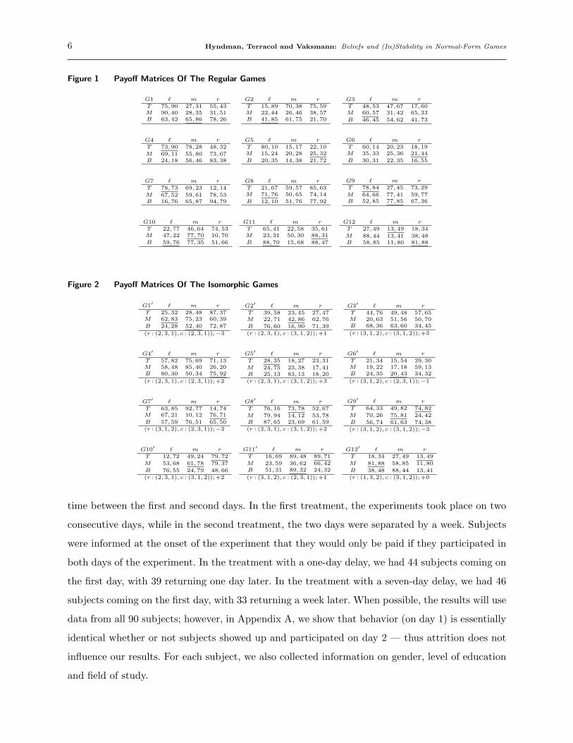
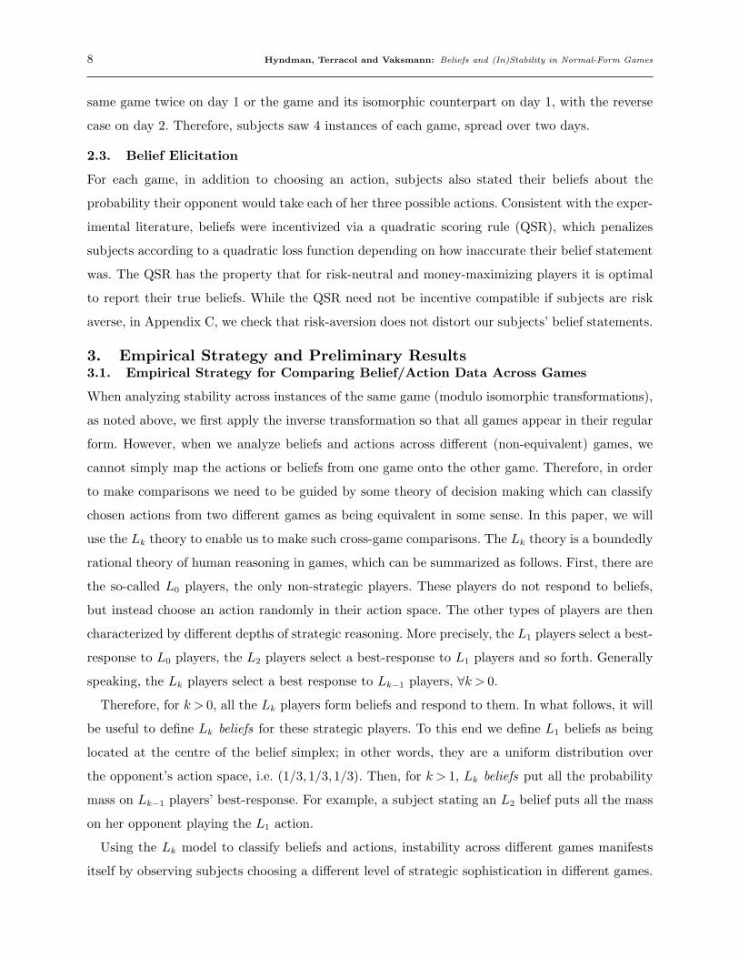
In order to do this, we designed the 12 games shown in Figure 1. These games were chosen with
the following properties: four of them had a unique Nash equilibrium that was in pure strategies
(games G1 to G4), four of them had a unique Nash equilibrium that could be arrived at through
the iterated deletion of dominated strategies (games G5 to G8) and four of them had two pure
strategy Nash equilibria (games G9 to G12). Because we were interested in whether behaviour is
sensitive to the frame, we also created 12 isomorphic games by interchanging rows and/or columns
and adding or subtracting a constant to the payoffs (cf. Figure 2). Note also that none of the games
have any mixed strategy Nash equilibria.3
In Figures 1 and 2 we underline the outcomes corresponding to Nash equilibria, and below
each payoff matrix in Figure 2 we describe how the game was transformed based on its regular
counterpart. For example, in game G1′, r : (2,3,1) indicates that row player’s first, second and third
actions appear in G1 as the second, third and first actions respectively. The notation, c : (2,3,1), is
analogous for column players. Finally, the −3 indicates that all payoffs were reduced by 3 points in
game G1′ relative to game G1. Unless otherwise noted, in our subsequent data analysis, to facilitate
the comparison of actions and beliefs between the regular and transformed games, we first apply
the inverse transformations so that all games appear in their regular form (i.e., as in Figure 1).
2.2. Procedures
Our experiments were run at the Parisian Lab for Experimental Economics (LEEP). Our subjects
were recruited among a broad pool of students from the University of Paris 1. The experiment
had two treatments. For both treatments, the experiment took place over two days, with identical
procedures on each day. The only distinguishing factor between the treatments was the length of
3 In contrast, many of the games in Costa-Gomes and Weizsacker (2008) had, in addition to the unique pure strategyequilibrium, two mixed strategy Nash equilibria. Although an analysis of their data did not find any evidence thatsubjects played any of the mixed strategy equilibria, we wanted our games to be as “clean” as possible and, therefore,made every effort to ensure that there were no mixed strategy equilibria.
6 Hyndman, Terracol and Vaksmann: Beliefs and (In)Stability in Normal-Form Games
Figure 1 Payoff Matrices Of The Regular Games
G1 ℓ m r
T 75,90 27,31 55,43M 90,40 28,35 31,51B 63,42 65,86 78,26
G2 ℓ m r
T 15,89 70,38 75,59M 22,44 26,46 38,57B 41,85 61,75 21,70
G3 ℓ m r
T 48,53 47,67 17,60M 60,57 31,42 65,33
B 46,45 54,62 41,73
G4 ℓ m r
T 73,90 78,28 48,32
M 69,11 55,80 73,67B 24,18 56,46 83,38
G5 ℓ m r
T 80,10 15,17 22,10M 15,24 20,28 25,32
B 20,35 14,38 21,72
G6 ℓ m r
T 60,14 20,23 18,19M 35,33 25,36 21,44
B 30,31 22,35 16,55
G7 ℓ m r
T 78,73 69,23 12,14
M 67,52 59,61 78,53B 16,76 65,87 94,79
G8 ℓ m r
T 21,67 59,57 85,63M 71,76 50,65 74,14
B 12,10 51,76 77,92
G9 ℓ m r
T 78,84 27,45 73,29
M 64,66 77,41 59,77B 52,85 77,85 67,36
G10 ℓ m r
T 22,77 46,64 74,53M 47,22 77,70 10,70
B 59,76 77,35 51,66
G11 ℓ m r
T 65,41 22,58 35,61M 23,31 50,30 88,31
B 88,70 15,68 88,47
G12 ℓ m r
T 27,49 13,49 18,34
M 88,44 13,41 38,48B 58,85 11,80 81,88
Figure 2 Payoff Matrices Of The Isomorphic Games
G1′ ℓ m r
T 25,32 28,48 87,37M 62,83 75,23 60,39
B 24,28 52,40 72,87
(r : (2,3,1), c : (2,3,1));−3
G2′ ℓ m r
T 39,58 23,45 27,47M 22,71 42,86 62,76
B 76,60 16,90 71,39(r : (2,3,1), c : (3,1,2));+1
G3′ ℓ m r
T 44,76 49,48 57,65M 20,63 51,56 50,70B 68,36 63,60 34,45
(r : (3,1,2), c : (3,1,2));+3
G4′ ℓ m r
T 57,82 75,69 71,13M 58,48 85,40 26,20B 80,30 50,34 75,92
(r : (2,3,1), c : (2,3,1));+2
G5′ ℓ m r
T 28,35 18,27 23,31
M 24,75 23,38 17,41B 25,13 83,13 18,20(r : (2,3,1), c : (3,1,2));+3
G6′ ℓ m r
T 21,34 15,54 29,30M 19,22 17,18 59,13B 24,35 20,43 34,32
(r : (3,1,2), c : (2,3,1));−1
G7′ ℓ m r
T 63,85 92,77 14,74M 67,21 10,12 76,71
B 57,59 76,51 65,50(r : (3,1,2), c : (2,3,1));−2
G8′ ℓ m r
T 76,16 73,78 52,67
M 79,94 14,12 53,78B 87,65 23,69 61,59(r : (2,3,1), c : (3,1,2));+2
G9′ ℓ m r
T 64,33 49,82 74,82
M 70,26 75,81 24,42
B 56,74 61,63 74,38(r : (3,1,2), c : (3,1,2));−3
G10′ ℓ m r
T 12,72 49,24 79,72
M 53,68 61,78 79,37
B 76,55 24,79 48,66(r : (2,3,1), c : (3,1,2));+2
G11′ ℓ m r
T 16,69 89,48 89,71
M 23,59 36,62 66,42B 51,31 89,32 24,32
(r : (3,1,2), c : (2,3,1));+1
G12′ ℓ m r
T 18,34 27,49 13,49
M 81,88 58,85 11,80
B 38,48 88,44 13,41(r : (1,3,2), c : (3,1,2));+0
time between the first and second days. In the first treatment, the experiments took place on two
consecutive days, while in the second treatment, the two days were separated by a week. Subjects
were informed at the onset of the experiment that they would only be paid if they participated in
both days of the experiment. In the treatment with a one-day delay, we had 44 subjects coming on
the first day, with 39 returning one day later. In the treatment with a seven-day delay, we had 46
subjects coming on the first day, with 33 returning a week later. When possible, the results will use
data from all 90 subjects; however, in Appendix A, we show that behavior (on day 1) is essentially
identical whether or not subjects showed up and participated on day 2 — thus attrition does not
influence our results. For each subject, we also collected information on gender, level of education
and field of study.

Hyndman, Terracol and Vaksmann: Beliefs and (In)Stability in Normal-Form Games 7
On each day, subjects played the games as given in Table 1 (though the order in which the games
were played differs from the presentation in the table).4 Subjects were given the role of either a
row player or a column player and kept that role for the entire experiment. For each game that
subjects played, they were randomly matched with another subject of the opposite role. In each
game, subjects had to complete two tasks: they had to state beliefs about the likely action that
their opponent would play; and to choose an action.
Table 1 Properties of Games
(a) Day 1
Game # Occ DS?Row Player Column Player
L1 L2 Nash L1 L2 Nash
G1 × 2 N B M B ℓ m m
G2 × 1 N T B B ℓ ℓ ℓ
G2′ × 1 N B M M m m m
G3 × 2 N M B M m ℓ ℓ
G4 × 1 N T T T m ℓ ℓ
G4′ × 1 N B B B ℓ r r
G5 × 2 Y T M M r m r
G6 × 1 Y T M M r m r
G6′ × 1 Y M B B m ℓ m
G7 × 2 Y M T M ℓ m ℓ
G8 × 1 Y M T M m ℓ ℓ
G8′ × 1 Y T B T r m m
G9 × 2 N M T T,B ℓ r ℓ, r
G10 × 1 N B T M,B r ℓ ℓ,m
G10′ × 1 N M B M,T ℓ m m,r
G11 × 2 N B M M,B m ℓ ℓ, r
G12 × 1 N B M T,B ℓ r m, r
G12′ × 1 N M B T,M m ℓ ℓ, r
(b) Day 2
Game # Occ DS?Row Player Column Player
L1 L2 Nash L1 L2 Nash
G1 × 1 N B M B ℓ m m
G1′ × 1 N M T M r ℓ ℓ
G2′ × 2 N B M M m m m
G3 × 1 N M B M m ℓ ℓ
G3′ × 1 N B T B r m m
G4′ × 2 N B B B ℓ r r
G5 × 1 Y T M M r m r
G5′ × 1 Y B T T ℓ r ℓ
G6′ × 2 Y M B B m ℓ m
G7 × 1 Y M T M ℓ m ℓ
G7′ × 1 Y B M M r ℓ r
G8′ × 2 Y T B T r m m
G9 × 1 N M T T,B ℓ r ℓ, r
G9′ × 1 N B M M,T m ℓ m,r
G10′ × 2 N M B M,T ℓ m m,r
G11 × 1 N T B M,B ℓ r ℓ, r
G11′ × 1 N T B T,B ℓ r m, r
G12′ × 2 N M B T,M m ℓ ℓ, r
# Occ: Number of times subjects saw the game on a given day.DS?: Is the game dominance solvable (Y) or not (N)?
After subjects made all of their choices on both days, they were paid according to their total game
payoffs and earnings from their belief statements. Earnings were denoted in experimental currency
units and were converted to Euros at the end to the rate of e0.75 for every 100 experimental units.
On average, subjects who came on both days earned e19.80.
Because we wanted to create as true as possible a series of one-shot games, and to mitigate
any learning effects, subjects did not receive any feedback regarding the action chosen by their
opponent or their payoffs for either actions of beliefs until the end of the experiment on the second
day. Appendix B checks for any hint of learning in our data and finds none. As can be seen in
Table 1, for each of the 12 sets of strategically equivalent games, subjects either saw the exact
4 More precisely, we randomized the presentation of games within a day with the only constraint being that theremust be at least three periods between instances of the same game.
8 Hyndman, Terracol and Vaksmann: Beliefs and (In)Stability in Normal-Form Games
same game twice on day 1 or the game and its isomorphic counterpart on day 1, with the reverse
case on day 2. Therefore, subjects saw 4 instances of each game, spread over two days.
2.3. Belief Elicitation
For each game, in addition to choosing an action, subjects also stated their beliefs about the
probability their opponent would take each of her three possible actions. Consistent with the exper-
imental literature, beliefs were incentivized via a quadratic scoring rule (QSR), which penalizes
subjects according to a quadratic loss function depending on how inaccurate their belief statement
was. The QSR has the property that for risk-neutral and money-maximizing players it is optimal
to report their true beliefs. While the QSR need not be incentive compatible if subjects are risk
averse, in Appendix C, we check that risk-aversion does not distort our subjects’ belief statements.
3. Empirical Strategy and Preliminary Results3.1. Empirical Strategy for Comparing Belief/Action Data Across Games
When analyzing stability across instances of the same game (modulo isomorphic transformations),
as noted above, we first apply the inverse transformation so that all games appear in their regular
form. However, when we analyze beliefs and actions across different (non-equivalent) games, we
cannot simply map the actions or beliefs from one game onto the other game. Therefore, in order
to make comparisons we need to be guided by some theory of decision making which can classify
chosen actions from two different games as being equivalent in some sense. In this paper, we will
use the Lk theory to enable us to make such cross-game comparisons. The Lk theory is a boundedly
rational theory of human reasoning in games, which can be summarized as follows. First, there are
the so-called L0 players, the only non-strategic players. These players do not respond to beliefs,
but instead choose an action randomly in their action space. The other types of players are then
characterized by different depths of strategic reasoning. More precisely, the L1 players select a best-
response to L0 players, the L2 players select a best-response to L1 players and so forth. Generally
speaking, the Lk players select a best response to Lk−1 players, ∀k > 0.
Therefore, for k > 0, all the Lk players form beliefs and respond to them. In what follows, it will
be useful to define Lk beliefs for these strategic players. To this end we define L1 beliefs as being
located at the centre of the belief simplex; in other words, they are a uniform distribution over
the opponent’s action space, i.e. (1/3,1/3,1/3). Then, for k > 1, Lk beliefs put all the probability
mass on Lk−1 players’ best-response. For example, a subject stating an L2 belief puts all the mass
on her opponent playing the L1 action.
Using the Lk model to classify beliefs and actions, instability across different games manifests
itself by observing subjects choosing a different level of strategic sophistication in different games.

Hyndman, Terracol and Vaksmann: Beliefs and (In)Stability in Normal-Form Games 9
3.2. Beliefs and Best-Response Behaviour
3.2.1. Typology of Beliefs. Table 2(a) shows the mean and standard deviation of beliefs
according to their original labels (i.e., in the form exactly as presented to the subjects). From
this, it would seem that subjects are not sensitive to labels when stating their beliefs: none of
the average beliefs are significantly different from 33 1/3. On the other hand, Table 2(b) shows
the mean and standard deviation of beliefs towards the opponent’s L1, L2, and “other” action,
respectively denoted bL1, bL2
and bOA in the table (for games/roles where the opponent’s L1 and
L2 actions differ). It indicates that beliefs are biased towards the opponent’s L1 action, and away
from the “other” action.5 The average belief towards the L1 action is significantly higher than 33
1/3, while the belief towards the “other” action is significantly lower than 33 1/3.
Table 2 Summary statistics
(a) Raw Data
Variable Mean Std. Dev. Std. Err.b1 33.232 26.827 0.717b2 33.034 24.646 0.489b3 33.735 25.675 0.728N 3836
(b) Organized by Lk Theory
Variable Mean Std. Dev. Std. Err.bL1
44.155 26.546 0.980bL2
32.398 24.262 0.793bOA 23.447 22.031 0.863N 3512
Standard errors clustered at the individual level.
Figure 3 shows the density of beliefs in the Lk simplex using the reflection method described
in Haruvy (2002). The white dot indicates L1 beliefs; while the gray dot indicates the location of
the maximum estimated density, which is located at (33,35,32). The figure shows that the largest
mode is, by far, at L1 beliefs. A secondary mode can be found at L2 beliefs. Lower modes also
appear at (.5, .5,0), L3 beliefs and (0,0,1). Outside these archetypal beliefs, most of the mass of
the distribution can be found around the segment joining L1 and L2 beliefs, explaining the higher
mean of beliefs towards the opponent’s L1 action.
We also find that the belief toward the opponent’s Nash action (in the set of games with a single
Nash equilibrium) is somewhat high at 39.8%. However, we do not think that players actually use
Nash equilibrium when stating their beliefs. Indeed, in our games the Nash action is always either
the L1 or the L2 action with roughly equal probabilities. If players had the Nash model in mind,
then their beliefs towards the Lk action should be higher when it coincides with the Nash action. To
test this prediction, we run OLS regressions clustered at the individual level of the beliefs towards
5 Note that the “other action” is rarely a Nash action, and when it is, it is one of two Nash equilibrium actions inthe multiple equilibria games.

10 Hyndman, Terracol and Vaksmann: Beliefs and (In)Stability in Normal-Form Games
Figure 3 Lk beliefs
0 20 40 60 80 100
020
40
60
80
100
Beliefs for L1 action
Belie
fs for
L2 a
ction
4e−05
4e−05
4e−05
4e−05 6e−05
6e−05
6e−05
8e−05
8e−05
1e−04
1e−04
1e−04
1e−04
0.00012
0.00012
0.00014
0.00014
0.00016
0.00018
2e−04
2e−04
0.00022
0.00024
0.00026
0.00026
0.00028
0.00028
3e−04
3e−04
3e−04
0.00032
0.00034
0.00036
0.00038
4e−04
0.00042
0.0
0044
5e−04
0.00052
0.00054
0.00056 0.00062 0.0
0064
7e−04
0.0
0072
8e−04
9e−04 ● ●
Belief t
oward
s th
e L1 a
ctio
nBelief towards the L2 actionD
ensity
Table 3 Frequency of Action Choices Organized by Level k Theory
Action Frequency Std. Dev. NL1|notL2 0.524 0.500 3512L2|notL1 0.356 0.474 3512L1 andL2 0.784 0.412 324
Other Action 0.129 0.356 3836
the L1 action on a dummy for coincidence between L1 and Nash.6 The associated coefficient is
0.068 with a p−value of 0.962. A similar regression for L2 beliefs leads to a coefficient of 2.175 and
a corresponding p−value of 0.1. We thus conclude that players do not use the Nash model when
forming their beliefs, or do so in a very marginal way.
3.2.2. Typology of Actions. In Table 3, we show the frequency with which the L1, L2 and
other actions were chosen overall in our experiment. Observe that the L1 action is chosen 52.4% of
the time, with the L2 action being chosen only 35.6% of the time. Taking the subject average as
the unit of independent observation, a paired t−test easily rejects the null hypothesis that these
frequencies are equal (p≪ 0.01). Thus it seems that most subjects choose the L1 action, with fewer
subjects choosing the L2 action and a small frequency of choices which are neither L1 nor L2.
3.2.3. Best-Response Behaviour. The overall rate of best-response is 62.6%, which is com-
parable to the best-response rate reported in Danz et al. (2012), but higher than those reported by
Costa-Gomes and Weizsacker (2008). Note also that unlike Costa-Gomes and Weizsacker (2008),
6 We restrict our sample to games with a unique equilibrium and for which the opponent’s L1 and L2 actions differ.

Hyndman, Terracol and Vaksmann: Beliefs and (In)Stability in Normal-Form Games 11
there are fairly pronounced differences in the best-response rate depending on where a subject’s
beliefs lie in the simplex. Figure 4(a) shows the results of a bivariate non-parametric regression of
the probability to give a best-response on the beliefs towards the opponent’s L1 and L2 actions.
First, it shows that when beliefs lie in a corner of the simplex, subjects exhibit a higher tendency
to best-respond to them, with an estimated best-response rate ranging from 0.7 to 0.85. Second,
subjects are also more likely to best-respond to beliefs that are near the L1 beliefs. Finally, the
lowest best-response rate is attained close to (0.60,0.05,0.35) beliefs.
Figure 4 Best-response behaviour
(a) Non-Parametric Regression
Belief L1
0 20 40 60 80 100
Belie
f L2
0
20
40
60
80
100
Pre
dic
ted p
robability
0.5
0.6
0.7
0.8
(b) Fixed-Effects Regression
Variable Coefficient (Std. Err.)1(bL1
≥ 0.85) 0.273† (0.155)1(bL2
≥ 0.85) 1.163∗∗ (0.242)1(bOA ≥ 0.85) 0.941∗∗ (0.256)1(d(b, bu)≤ 0.075) 0.422∗∗ (0.123)
N 3512Log-likelihood -1854.51χ2(86) 250.986
Significance levels : † : 10% ∗ : 5% ∗∗ : 1%
To see this more parametrically, in Figure 4(b) we report the results of a conditional fixed-effects
logistic regression of “choosing a best-response” on dummies for having beliefs near the corners of
the simplex (i.e., when the belief to the L1 action, the L2 action or another action exceeds 0.85)
and “being close to the uniform L1 beliefs” (bu) with a full set of game, day and period dummies.7
Just as shown in Figure 4(a), having strong beliefs increases the rate of best-response.
3.3. A First Look at Belief and Action Stability
We now turn our attention to both belief and action stabilities. If subjects have a consistent and
stable theory of the mind of their opponents, then they should report similar beliefs and choose
equivalent actions in different instances of the same game. To get an initial feel for the beliefs
7 We define closeness to L1 beliefs based on the Euclidean distance to L1 beliefs, taking value 1 if the beliefs arecontained in a ball of radius 0.075 centred on L1 beliefs.

12 Hyndman, Terracol and Vaksmann: Beliefs and (In)Stability in Normal-Form Games
data, Figure 5 displays, in its lower panel, the histogram of current beliefs and, in its upper panel,
the histograms of the beliefs in the next instance of a strategically equivalent game conditional on
current beliefs lying in the corresponding interval.8 Note that this figure captures our first degrees
of stability: within identical or strategically equivalent strategic games.
Figure 5 Belief stability
010
20
30
40
50
60
70
80
90
100
Belie
f in
next in
sta
nce
.1 .3 .5 .1 .3 .5 .1 .3 .5 .1 .3 .5 .1 .3 .5 .1 .3 .5 .1 .3 .5 .1 .3 .5 .1 .3 .5 .1 .3 .5
0.0
5.1
.15
.2F
raction
[0,10) [10,20) [20,30) [30,40) [40,50) [50,60) [60,70) [70,80) [80,90) [90,100]Belief in current instance
It is clear from Figure 5 that stated beliefs are fairly stable across instances of the same game.
With the exception of the interval [70,80) (which accounts for only 3% of statements), the modal
belief interval in the next instance is equal to the same interval in which the belief the current
belief lies (shown in a darker shade).
The same pattern can be found for actions. Table 4 shows, for each type of action in the current
instance of a game (rows of Table 4), the distribution of actions in the next instance of the same
game. As with beliefs, the modal action in the next instance is equal to the action chosen in the
current instance. The overall frequency of identical actions being chosen in consecutive instances
8 In this figure we pool the beliefs towards each of the opponent’s three possible actions.

Hyndman, Terracol and Vaksmann: Beliefs and (In)Stability in Normal-Form Games 13
is 0.662, well above random behavior. Table 4 also reveals a clear hierarchy among actions, with
L1 being the most stable, followed by L2. The “other” action is the least stable, which may reveal
that some of these were errors corrected in the next instance of the same game.
Table 4 Action stability
Action in the next instanceL1 action L2 action Other action Total
L1 action 0.729 0.209 0.062 1L2 action 0.306 0.621 0.069 1Other action 0.273 0.258 0.469 1
3.3.1. An Index of Belief Stability in Terms of Best-Response. A rough, but useful
way to study the stability of beliefs is to look at the differences between the four best-response sets
implied by subjects’ belief statements in the four instances of each game.9
Let bsg denote the elicited beliefs of a subject playing the sth instance of game g, and denote
by BRg(bsg) the best-response set for these beliefs (recall that we converted all games back to
their original frame, so that belief statements are comparable across all four instances of a game).
We can distinguish between four different levels of stability across four instances of each game.10
Specifically, dropping the game subscript, g, for simplicity:
(i) For all s, t ∈ {1,2,3,4} BR(bs) = BR(bt). This is the most stable case in which a subject’s
belief statements imply identical best-response sets across all four instances of the game. This
is given an index value of 4.
(ii) There exists a unique instance, s, such that BR(bs) 6=BR(bt), while for all t, t′ 6= s, BR(bt) =
BR(bt′
). In this case, a subject’s statements imply identical best-response sets in 3 out of the
4 instances of the game. This is given an index value of 3.
(iii) For each instance s, there is a unique instance t 6= s such that BR(bs) =BR(bt). That is, over
all four instances, there are two different best-response sets, each set occurring twice. This is
given an index value of 2.
(iv) There exists a unique pair (s, t) such that BR(bs) =BR(bt) and for any other pair of instances
(t′, t′′) 6= (s, t), BR(bt′
) 6= BR(bt′′
). That is, the subject’s best-response sets coincided in two
instances, and differed in every other instance. This is given an index value of 1.
9 Therefore, results presented here (and subsequently when we look at action stability) excludes those subjects whoonly participated on the first day. However, in Appendix A we show that there are no significant differences inbehavior between subjects who participated on both days and those who only participated on the first day.
10 Because the best-response set need not be a singleton, it is possible that the best-response sets differ across all fourinstances; however, this was never observed in our data.

14 Hyndman, Terracol and Vaksmann: Beliefs and (In)Stability in Normal-Form Games
Table 5 Distribution of the beliefs stability index against random beliefs
Game classindex DSG MEQ nDSG Overall
Actual Random (U) Actual Random (U) Actual Random (U) Actual Random (U)1 3.93 9.91 2.08 12.05 2.43 10.81 2.80 10.922 17.14 16.33 12.50 21.27 16.67 20.81 15.42 19.473 36.43 36.71 28.47 38.79 33.68 41.76 32.83 39.094 42.50 37.05 56.94 27.89 47.22 26.62 48.95 30.52
Table 5 presents the distribution of the stability index separately for each class of games, as well
as pooling across classes. For each class, the first column displays the observed distribution of the
index, while the second shows the distribution that would be observed if players chose their beliefs
randomly.11 Overall, subjects have the highest value of our index in half of the games, and err more
than once in only about 18% of the games, which indicates fairly high belief stability within the
same game. The highest value of the index is markedly more prevalent in the actual data compared
to random belief statements, although less so for the set of dominance solvable games.
We next run a series of χ2 tests of the empirical distribution of the index against the random
statements distribution. The tests are run separately for each game and role so that the observations
are independent within each test. The observed distribution of the index is significantly different
from the random statements distribution for 19 (resp. 17) out of the 24 comparisons at the 10%
(resp. 5%) level of significance.12 It is also clear from Table 5 that different game classes lead to
different degrees of stability. To test this more formally, we define “excess stability” as the difference
between the actual value of the index and the expected value under random statements.13 We then
run paired t−tests at the individual level (N = 72) using the individual average excess stability for
each game class. MEQ games have the highest excess stability (0.571) followed by nDSG games
(0.424) and finally DSG games (0.178). The paired t−tests reveal that differences between all three
pairs of game classes are significant at the 5% level. Thus subjects have significantly more stable
beliefs in MEQ games and beliefs are least stable in DSG games.
11 This distribution was obtained by drawing uniform random beliefs over the simplex for 20000 players (10000rows and 10000 columns) for 4 occurrences in each set of strategically equivalent games, and by calculating thecorresponding index.
12 We fail to reject at the 10% level of significance in games 2, 3, 6 and 8 (row players) and game 6 (column players),while at the 5% level we also fail to reject the null hypothesis for games 6 (column) and 9 (row).
13 More precisely, our measure of excess stability for a given set of strategically equivalent games played by a givenindividual is the difference between the observed index and the expected index under random statements for thecorresponding game×role.

Hyndman, Terracol and Vaksmann: Beliefs and (In)Stability in Normal-Form Games 15
3.3.2. An Index of Action Stability. Just as with beliefs, we can construct an index of
action stability. The principle of this new index is the same. Specifically, we quantify how many
times, across all four instances of the same game, a subject’s actions coincided (recall that we
converted all games back to their original frame, so that action choices are comparable across all
four instances). Let xsg denote the action chosen by a subject in the sth instance of game g. There
are four different levels of stability. Specifically, dropping the game subscript, g, for simplicity:
(i) ∀s, t ∈ {1,2,3,4}, xs = xt. This is the most stable case in which a subjects chooses the same
action in all four instances. This is given an index value of 4.
(ii) There exists a unique instance, s, such that for all t 6= s, xs 6= xt, while for all t, t′ 6= s, xt = xt′ .
In this case, a subject takes the same action in three of four instances. This is given an index
value of 3.
(iii) For each instance s, there exists a unique instance t 6= s such that xt = xs. That is, over all
four instances, a subject chose two different actions and each action was played twice. This is
given an index value of 2.
(iv) There exists a unique pair (s, t) such that xs = xt and for any other pair of instances (t, t′′) 6=
(s, t), xt 6= xt′ . This is the least stable case in which a subject chose all three actions, by
necessity repeating the same action twice. This is given an index value of 1.
The distribution of the action stability index separated by class of games is given in Table 6.14
Table 6 Distribution of the action stability index
Game classindex DSG MEQ nDSG Overall Random1 11.07 4.86 10.42 8.76 44.42 17.14 13.19 17.01 15.77 22.23 36.43 36.46 37.85 36.92 29.64 35.36 45.49 34.72 38.55 3.7
As can be seen, the actual distribution of the index shows substantially more stable behavior than
implied by randomness. The χ2 tests of equality of the empirical and random uniform distribution
of the index give p≤ 0.001 in all 24 comparisons. Again, we can also test whether action stability
differs by game class. Paired t−tests at the individual level reveal that MEQ games are significantly
more stable than both DSG (p≪ 0.01) and nDSG (p≪ 0.01) games, but that DSG and nDSG
games do not differ along the stability dimension (p= 0.85).
14 The distribution of the actions stability index under randomness is identical across classes as it does not dependon the payoffs of the game.

16 Hyndman, Terracol and Vaksmann: Beliefs and (In)Stability in Normal-Form Games
3.3.3. The Relationship Between Belief and Action Stability. To assess if stability in
beliefs is related to stability in actions, we run a fixed-effects regression of stability in actions on
stability in beliefs, controlling for a full set of game dummies and clustering the standard errors
at the individual level. The estimated coefficient is 0.212, with a p−value < 0.001. Running the
same fixed effects regression but using our measure of excess stability as an explanatory variable
leads to a coefficient of 0.11 with a p−value of 0.011. Our two measures are thus positively and
significantly related: higher belief stability is associated with a higher action stability.
4. A Deeper Look at Stability4.1. A Deeper Look at Belief Stability
In this section, we focus on the determinants of belief stability, and on the relation between stability
within instances of the same game and stability across different games. To do so, we compute the
Euclidean distance in ❘3 between belief statements. When studying the stability within the same
game, we take the distance between belief statements in two consecutive instances of the same
game. When studying stability across different games, we compute the distance between belief
statements in two consecutive periods in the experiment, which correspond to different games. In
the latter case, the coordinates are defined in the Lk simplex. Both distances are normalized so
that the maximum distance attainable from a given belief is given a value of 1.
The average normalized distance between belief statements in two consecutive instances of the
same game is 0.276. The first quartile is 0.097, the median is 0.208, and the third quartile is 0.378.
Thus, 50% of distances between beliefs are below a fifth of the maximal distance that could be
observed, i.e. moving to a (different) vertex of the simplex. Random belief statements over the
simplex would lead to an expected distance of 0.456. A t−test at the individual level reveals that
the observed distance between beliefs in instances of the same game is significantly lower than
what would have happened under randomness (t=−15.34, p≪ 0.01).
We now explore how time and framing affects the distance between stated beliefs. Table 7(a)
shows the results of paired t−tests for the equality of normalized distance in beliefs for consecutive
instances in the same game. The first cell of Table 7(a) states that the normalized distance in
beliefs to equivalent actions when the consecutive instances are played with a 1 day delay is 0.274,
while it is 0.242 when the instances are played on the same day. The corresponding p−value is
0.006. All tests are performed using individual means as the unit of observation. As can be seen
from Table 7(a), time has a statistically significant impact on the distance between consecutive
belief statements, although its quantitative effect is rather small, with a one week delay adding
less than 15% to the average distance compared to games played on the same day.

Hyndman, Terracol and Vaksmann: Beliefs and (In)Stability in Normal-Form Games 17
Table 7 Belief Stability: The Effects of Time and Framing
(a) The Effect of Time
Time delay t= 1 t= 7 t.d.≥ 1∆= t 0.274 0.307 0.292∆= 0 0.242 0.268 0.256
p−values 0.006 0.001 0.000N 33 39 72
(b) The Effect of Framing (i.e., isomorphic transformation)
Isomorphic ∆= 0 ∆= 1 ∆= 7 ∆≥ 1 OverallNo 0.242 0.256 0.301 0.280 0.254Yes 0.270 0.285 0.311 0.299 0.281
p−values 0.041 0.405 0.624 0.331 0.024N 72 33 39 72 72
Table 7(b) shows the results of paired t−tests for the difference in normalized distance for
consecutive instances of the same game between pairs that are isomorphic transformations and
pairs that are identical. We run the tests on the subsample of subjects that were present on both
days of the experiment. The entry in the first row gives the average distance in consecutive beliefs
when the instances have identical frames, while the second row gives the distance in beliefs when
the instances are isomorphic transformations; the third row give the p−value of the test. ∆ refers
to the number of days between the two consecutive instances.
While isomorphic transformations have a statistically significant impact when instances are
played on the same day, its impact fade when instances are played on different days. The difference
in average distances is also rather small (around 10% of the mean distance).
Table 8 presents the results of an OLS regression of normalized Euclidean distance between
belief statements to equivalent actions in consecutive instances of the same game on a dummy
for isomorphic transformation, dummies for time between statements (and their interactions), as
well as dummies for game class. Standard errors are clustered at the individual level. Isomorphic
transformation has a small significant impact on the distance, as well as having a 7-day delay
between plays. Consistent with our previous results, but surprising nonetheless is the fact that
DSG games appear to be the least stable.
We now investigate stability of Lk beliefs, and its relation to within game stability. The average
normalized distance in the Lk simplex between belief statements in consecutive games with different
strategic structures is 0.374. As was the case for within game stability, this is significantly smaller
than the distance implied by random statements (t = −5.33, p≪ 0.01). Note also that a paired
t−test at the individual level reveals the mean distance between stated beliefs in consecutive
instances of the same game are significantly smaller than the mean distance in consecutive games
with different strategic structures (0.276 vs 0.374; p≪ 0.01). Thus, subjects tend to cluster their
beliefs more when facing the same game than when facing a strategically different game.
Figure 6(a) shows the scatterplot of average distance between consecutive games with different
strategic structures against average distance in consecutive instances of the same game, individuals

18 Hyndman, Terracol and Vaksmann: Beliefs and (In)Stability in Normal-Form Games
Table 8 Belief stability within sets of strategically equivalent games
Variable Coefficient (Std. Err.)Isomorphic change 0.026∗ (0.012)∆day=1 0.020 (0.022)∆day=7 0.047∗ (0.023)Isomorphic change×∆day=1 -0.019 (0.032)Isomorphic change×∆day=7 -0.005 (0.025)MEQ -0.026∗ (0.012)nDSG -0.040∗∗ (0.011)Intercept 0.271∗∗ (0.014)
N 2774R2 0.011F (7,89) 4.042Significance levels : † : 10% ∗ : 5% ∗∗ : 1%
that are closer to the centre of the simplex are shown using a darker shading. Individuals who tend
to report beliefs close to the centre of the simplex also tend to have relatively stable beliefs, both
within and between sets of strategically equivalent games; and the relation between both stabilities
is strong. As the average distance to the centre increases, both kind of stabilities decrease, and the
relation between the two gets noisier.
Figure 6 Within and between stability
(a) Scatter Plot
●
●●
●
●●
●
●
●
●
●
●
●
●
●
●
●
●●
●
●
●
●
●
●
●
●
●
●●
●
●
●
●
●
●
●
●
●
●
●
●
●
●
●
●
●
●
●
●●●
●
●
●
●
●●
● ●
●
●●●
●
●
●
●
●
●
●
●
●
●
●
●
●
●
●
●
●
●
●
●
●
●
●
●
●
●
0.0 0.1 0.2 0.3 0.4 0.5 0.6
0.0
0.1
0.2
0.3
0.4
0.5
0.6
0.7
Average distance between consecutive instances
Avera
ge d
ista
nce b
etw
een c
onsecutive g
am
es
Min. Med. Max.
Aver. dist. to centre of simplex
(b) Regression Estimates
Variable Coefficient (Std. Err.)Av. dist. cons. inst. 0.348∗∗ (0.102)Av. dist. centre 0.531∗∗ (0.043)Intercept 0.056∗∗ (0.020)
N 90R2 0.847F (2,87) 199.308Significance levels : † : 10% ∗ : 5% ∗∗ : 1%
Figure 6(b) displays the results from an OLS regression of the average distance between consec-
utive games with different strategic structures on average distance between consecutive instances

Hyndman, Terracol and Vaksmann: Beliefs and (In)Stability in Normal-Form Games 19
of the same game and average distance to the centre of the simplex. Both coefficients are positive
and significant, confirming the insight from Figure 6(a).
To investigate further the within-game clustering of beliefs, we compute the overall centroid of
beliefs for each individual, as well as for each individual in each set of 12 games. We then compute
the Euclidean distance between each belief statement and the overall centroid; and between each
belief statement and the corresponding individual centroid in the set of strategically equivalent
games. We then compute the mean of the distance to the overall centroid, as well as the mean of the
distance to the centroid in the set of identical games. The individual-level average of the normalized
distance to the overall centroid is 0.399; and the mean normalized distance to the centroid in the
set of strategically equivalent games is 0.186. A paired t−test at the individual level (N=90) rejects
the null of equality of the two mean distances at the 1% level (t= 16.04; p≪ 0.01).
A multivariate ANOVA on the coordinates of the stated beliefs in the Lk simplex also reveals
that the within-individual variance in a set of strategically equivalent games is smaller than the
individual-level variance in the coordinates (F = 3.39; p≪ 0.01).
The results presented point to the fact that beliefs are fairly stable across different instances of
the same game, although time and isomorphic transformations have a small but significant impact
of belief stability. Moreover, subjects tend to report beliefs that are clustered by sets of strategically
equivalent games, with the distance between different games being higher than distances between
two instances of the same game. This suggests a model in which individuals pick a focal belief for
a given game and make belief statements as trembles around their beliefs. Subjects then may or
may not move to other focal beliefs in a different game. In Section 5 we estimate such a model.
4.2. A Deeper Look At Action Stability
Although actions possess a fair bit of stability within strategically equivalent games, we now seek
to understand whether there are any underlying causes for instability from one instance to the
next. To this end, in Table 9 we report the results of a fixed-effects (conditional) logit regression
where the dependent variable takes value 1 if the subject’s action changes from one instance to the
next. Game fixed effects were included in the estimation, but are not reported in the table.
As can be seen, the biggest determinant of whether a subject changes her action from one instance
to the next is a corresponding change in her best-response. This result lends further support to
our earlier claim that stability in beliefs and actions are closely related. We also see that subjects
who chose a best-response to their beliefs in the last instance are significantly less likely to change
their action in the current instance, and that subjects are somewhat less likely to change actions
in later instances. Whether the game was presented as an isomorphic transformation from the

20 Hyndman, Terracol and Vaksmann: Beliefs and (In)Stability in Normal-Form Games
Table 9 Why Do Actions Change Across Instances?
Variable Coefficient (Std. Err.)1(Chose a Best-response) -0.689∗∗ (0.092)1(∆Best-response) 0.785∗∗ (0.099)instance -0.112∗ (0.056)Isomorphic Change 0.077 (0.089)1(∆Day = 1) 0.089 (0.147)1(∆Day = 7) 0.119 (0.125)
N 2762LL -1369.12χ2(17) 182.49
Significance levels : † : 10% ∗ : 5% ∗∗ : 1%
previous instance or the delay from one instance to the next do not seem to have any impact on
the likelihood that subjects will change actions. All of these results seem to suggest that, for each
game, subjects are searching for the appropriate “model” of behaviour and that once they have
found it, their action choices become more stable.
As for beliefs, we can look at whether actions are stable across different games. Table 10 shows,
for each type of action in the current game, the distribution of actions in the next game that
subjects saw in the actual experiment (which was always strategically different). Comparing with
Table 4, we find that actions are substantially less stable across different games than within sets of
strategically equivalent games. The overall proportion of actions followed by an action of the same
type is 0.495, which is greater that what would have happened under randomness, but below the
0.662 found for consecutive instances of equivalent games. The L1 action is found to be the most
stable. In contrast, L2 and “other” Lk actions appear much more unstable as the modal following
action is not at the same level.
Table 10 Stability across games
Action in the next gameL1 action L2 action Other action Total
L1 action 0.607 0.305 0.088 1L2 action 0.452 0.419 0.129 1Other action 0.376 0.397 0.227 1
4.3. Stability, Accuracy and Best-Response
Do more stable beliefs lead to more predictive power of the opponents’ action? We construct a
variable which takes a value of 1 if the best-response set implied by the stated beliefs contains the
best-response to the opponent’s action and zero otherwise; and another which takes a value of 1 if

Hyndman, Terracol and Vaksmann: Beliefs and (In)Stability in Normal-Form Games 21
the action taken by the player is a best-response to the opponent’s action. We compute the average
of these variables over the 4 plays of each of our 12 games and regress these averages on dummies
for our stability index, clustering the standard errors at the individual level. Table 11 reports the
results and indicates that higher degrees of stability are associated with higher accuracy of stated
beliefs, with the lowest degree of stability being associated to a 33.3% — essentially a random
belief statement. The same pattern holds for accuracy of actions, except that the lowest stability
index is associated with a rate of correct actions below that of random choice. With actions, we
also have monotonicity: with higher stability being associated with higher predictive power.
Table 11 Accuracy and stability
Correct Best-response Correct actionVariable Coefficient (Std. Err.) Coefficient (Std. Err.)Index=2 0.182∗∗ (0.046) 0.143∗ (0.055)Index=3 0.149∗∗ (0.046) 0.183∗∗ (0.053)Index=4 0.232∗∗ (0.047) 0.255∗∗ (0.052)Intercept 0.333∗∗ (0.042) 0.281∗∗ (0.051)
N 856 856R2 0.024 0.032F (3,71) 10.35 10.858Significance levels : † : 10% ∗ : 5% ∗∗ : 1%
We now turn to the question of the link between stability and best-response behaviour. We run a
fixed-effects regression with clustered standard errors of the average propensity to best-respond in
each game on our indices of belief and action stability. We control for a full set of game dummies.
The results are displayed in Table 12 and show that the rate of best-response is increasing in both
action and belief stability. All in all, the links between stability, best-response and accuracy suggest
that stability is related to, if not intelligence, at least a greater focus on the tasks to be performed.
Table 12 Best-response vs indices
Variable Coefficient (Std. Err.)Actions stability index 0.097∗∗ (0.011)Beliefs stability index 0.041∗∗ (0.014)Intercept 0.226∗∗ (0.053)
N 856R2 0.163F (13,71) 12.15Significance levels : † : 10% ∗ : 5% ∗∗ : 1%

22 Hyndman, Terracol and Vaksmann: Beliefs and (In)Stability in Normal-Form Games
5. A Mover-Stayer Model
The descriptive analysis of Section 4.1 highlighted some stylized facts about belief stability within
and between sets of similar games. First, beliefs tend to be clustered within similar games, but less
so overall. Second, stability within sets of similar games and stability between sets of similar games
seemed to be positively correlated. In this section we construct and estimate a more structural
model to capture these features. We assume belief statements are really trembles around underlying
true beliefs (Costa-Gomes and Weizsacker 2008) and in which underlying beliefs may vary between
strategically different games. The degree to which subjects “tremble” when stating beliefs is allowed
to vary with their tendency to switch underlying beliefs between strategically different games.
5.1. Model and Results
Each individual i is a stayer (s) with probability ps, or a mover (m) with probability 1−ps. Stayers’
underlying beliefs are stable from game to game (i.e. they remain on the same level of thinking
regardless of the strategic structure of the game). Each stayer’s beliefs is one among Q possible
beliefs in the 2-simplex ∆2. Movers, on the other hand, choose one of the Q possible beliefs for each
set of identical games, and keep the same beliefs for every instance h ∈ Gg in this set, where, Gg
denotes the set of all games that are strategically equivalent to game g. Movers may change their
underlying beliefs between strategically different games. Stayers choose their beliefs according to
the probability distribution (p1s, . . . , pQs), while movers choose theirs according to the probability
distribution (p1m, . . . , pQm); where pqt stands for the probability that a type t player choose the qth
belief; pqt ≥ 0 and∑Q
q=1 pqt = 1, ∀q, t, q ∈ {1, . . . ,Q}, t ∈ {m,s}. Each actual belief statement is a
tremble around the underlying belief.
The density ditqj of player i’s belief statement in game g when she has the underlying qth belief
and her type is t∈ {m,s} is constructed as in Costa-Gomes and Weizsacker (2008):
ditqh =exp
(
λtνg(
big, bq))
∫
s∈∆2 exp (λtν (s, bq))ds, (1)
where big ≡ (big,1, big,2, b
ig,3) ∈∆2 is the belief statement player i reports in game g for each of her
three actions, bq is the qth belief. The term νg(
big, bq)
is the expected payoff obtained from the
quadratic scoring rule when true beliefs are bq and the belief statement is big. λt is a parameter to
be estimated, which captures players’ sensitivity to payoff differences. Specifically, when λt tends
to 0, type-t players choose their belief reports randomly on the simplex. Conversely, when λt tends
to ∞, underlying beliefs are stated without any noise.

Hyndman, Terracol and Vaksmann: Beliefs and (In)Stability in Normal-Form Games 23
The likelihood for the set of belief statements of individual i is thus:
li = ps∑
q
pqs∏
h
disqh +(1− ps)∏
g
∑
q
pqm∏
h∈Gg
dimqh. (2)
We set Q= 4, and set 3 of the 4 beliefs to be at the vertices of the Lk simplex: b2 ≡ (1,0,0); b3 ≡
(0,1,0) and b4 ≡ (0,0,1). The first type of belief, b1 ≡ (µ1, µ2, µ3 = 1−µ1 −µ2) is to be estimated
from the data.
We maximise the log-likelihood of our sample using the Nelder-Mead algorithm. We then run
one iteration of Newton-Raphson to get the variance-covariance matrix of the estimates using
the observed information matrix method. Final standard errors are obtained through the Delta
method. Results are displayed in Table 13.
Table 13 Mover-Stayer model
Description Parameter Estimate (Std. Err.)Fraction of stayers ps 0.285∗∗ (0.048)Movers, frac. interior p1m 0.197∗∗ (0.039)Movers, frac. L2 beliefs p2m 0.488∗∗ (0.031)Movers, frac. L3 beliefs p3m 0.217∗∗ (0.021)Movers, frac. other beliefs p4m 0.098∗∗ (0.006)Stayers, frac. interior p1s 0.989∗∗ (0.019)Stayers, frac. L2 beliefs p2s 0.000 (0.006)Stayers, frac. L3 beliefs p3s 0.001 (0.019)Stayers, frac. other beliefs p4s 0.000 (0.000)
Estimated interior beliefsµ1 0.426∗∗ (0.004)µ2 0.320∗∗ (0.004)µ3 0.253∗∗ (0.003)
Rationality parametersλm 0.263∗∗ (0.012)λs 2.243∗∗ (0.096)N 3512 (90 individuals)Log-likelihood -12238.921
Significance levels : † : 10% ∗ : 5% ∗∗ : 1%
About 28.5% of the individuals are stayers, and they overwhelmingly (99% of them) choose to
stay at the beliefs located inside of the Lk simplex, which we estimate to be at (0.426,0.320,0.253),
which is very close to the centre of the simplex (i.e., the L1 belief). Movers, on the other hand
hold beliefs that are more evenly distributed among the 4 types, with the L2 belief having the
highest (48%) probability to be chosen, followed by the L3 belief and inner belief (20% each) and
finally the last vertex of the simplex (10%). The overall distribution of underlying belief statements
implied by these estimates give the inner belief a lead with 42% of the statements, followed by the
L2 belief with 35%, then the L3 type with 16%, and lastly the last vertex with 7%. These figures

24 Hyndman, Terracol and Vaksmann: Beliefs and (In)Stability in Normal-Form Games
are consistent with the estimated densities given in Figure 3. Indeed, even though the estimated
densities seemed to give a larger difference between L1 and L2 beliefs, the fact that stayers (who
tend to have their beliefs located in the centre of the simplex) have a higher precision parameter
leads to a higher spike in the density than for the other beliefs, which are mainly chosen by movers
who have a much lower value of λ.
Note that given that stayers report very nearly L1 beliefs and the fact that the Quadratic
Scoring Rule favors uniform reports for risk-averse people, one might be tempted to argue that
stayers are risk averse. However, we argue against this interpretation in Appendix C. A risk averse
subject would state beliefs closer to the centre than her true belief. Assuming that she best-
responded to her true belief and not to her stated belief, this would create an inconsistency between
chosen actions and stated beliefs; that is, a risk averse subject should have a lower rate of best-
response. We find no support for this in our data. Instead stayers appear more simply to have quite
conservative/unsophisticated beliefs, but generally have the same rate of best-response.
5.2. Movers and Stayers
Using Bayes’ theorem and the estimated parameters of the mover-stayer model, one can compute
the posterior probabilities that a subject belongs to a given type of players. Namely, denoting by
(bit)t=1,...,48 the vector of subject i’s stated beliefs across the 48 games played; the probability that
i is a stayer given his observed statements can be written as:15
Pr(
stayer |(bit)t=1,...,48
)
=ps
∑
qpqs
∏
gdisqg
li. (3)
The distribution of the posterior probabilities of being a stayer is heavily concentrated around
0 and 1, as shown by Figure 7.
Using these posterior probabilities, we can assign each individual to either the mover or stayer
type. More precisely, we define the dummy variable:
stayeri := I(Pr(stayer |(bit)t=1,...,48)>0.5)
Based on this rule, our set of 90 subjects is composed of 27 stayers (30%) and 63 (70%) movers.
Figure 8 shows the density of stated beliefs in the Lk simplex separating by movers (above) and
stayers (below), which confirms that stayers have their beliefs concentrated on L1 beliefs; while
movers’ beliefs are more scattered, with highest mass at the L2 vertex, followed by the centre
15 For those subjects who did not come back on Day 2, and who consequently played 24 games, we use the vector(bit)t=1,...,24.

Hyndman, Terracol and Vaksmann: Beliefs and (In)Stability in Normal-Form Games 25
Figure 7 Posterior probabilities
020
40
60
80
Perc
ent
0 .2 .4 .6 .8 1Pr(Stayer|(b
it)t=1...48)
and the other vertices of the simplex. The empirical distribution of stayers’ and movers’ beliefs
is consistent with the estimation results of Table 13. Table 14 summarizes the relation between
assigned type/posterior probabilities and several measures of stability. Columns 2 and 3 show the
difference in the stability metric between movers and stayers and the corresponding p-value for
a t-test of equality. Columns 4 and 5 show the estimated coefficient of an OLS regression of the
metric on the posterior probability; and the p-value for the test that the coefficient is 0 (we used
robust standard errors). All tests confirm the higher stability of stated beliefs for those classified
as stayers by our model.
Table 14 Stability measures
By type By Pr (stayer)
Metric ∆ p-value β p-valueAv. dist. in successive instances of the same game -.145 < 10−3 -.148 < 10−3
Av. dist. in successive games from different sets of games -.186 < 10−3 -.188 < 10−3
Av. dist. to the centroid of the set of the same games -.100 < 10−3 -.101 < 10−3
Av. dist. to the overall centroid -.252 < 10−3 -.255 < 10−3
How do stayers fare relative to movers? Table 15 keeps the same structure as Table 14, but
shows results for several measures of performance: actions and beliefs (QSR) payoffs; rate of correct
best-response (i.e. the proportion of times their best-response set contained the best-response to
the actual opponent’s action), rate of correct actions (i.e. the proportion of times their action was
a best-response to the actual opponent’s action) and rate of best-response. While stayers do not
earn significantly more than movers in the action task, they do fare better than movers on the
belief task. Movers and stayers have the same rate of best-response, although stayers’ beliefs and
actions are significantly less often a result of a correct model of the mind of the opponents.

26 Hyndman, Terracol and Vaksmann: Beliefs and (In)Stability in Normal-Form Games
Figure 8 Movers’ and stayers’ beliefs
(a) Movers
0 20 40 60 80 100
02
04
06
08
01
00
Beliefs for L1 action
Be
liefs
fo
r L
2 a
ctio
n
6e−05
6e−05
6e−05
6e−05
8e−05
8e−05
8e−05
1e−04
1e−04
0.00012
0.00012
0.00014
0.00014
0.00014
0.00014
0.00014
0.00016
0.00016
0.00018
0.00018
2e−04
2e−04
0.00022
0.00022
0.00024
0.00024
0.00026
0.00028
0.00028
3e−04
3e−04
3e−04 0.00032
0.0
0032
0.00032
0.00032
0.00034
0.00034
0.0
0034
0.0
0036
0.00038
4e−04
4e−04
4e−04
0.0
0042
0.00042
5e−
04
0.00056
0.00064
●
Belief t
oward
s th
e L1 a
ctio
nBelief towards the L2 actionD
ensity
(b) Stayers
0 20 40 60 80 100
02
04
06
08
01
00
Beliefs for L1 action
Be
liefs
fo
r L
2 a
ctio
n
5e−05
5e−05
1e−04
0.00015
2e−04
0.00025
3e−04 0.00035 4e−04
0.00045
5e−04
0.00055
6e−04
0.00065 7e−04
0.00075
8e−
04
9e−04
0.00095
0.001
0.0
0105
0.0011
0.00115
0.0
0125
0.0014 0.0018 ●
Belief t
oward
s th
e L1 a
ctio
nBelief towards the L2 action
Density
Table 15 Performance
By type By Pr (stayer)
Metric ∆ p-value β p-valueAverage action payoff 1.21 0.181 1.290 0.161Average QSR payoff .560 < 10−3 .567 < 10−3
Rate of correct BR -0.085 0.0015 -0.087 0.001Rate of correct actions -0.066 0.017 -0.067 0.016Rate of best-response -0.027 0.3936 -0.026 0.412
Finally, stayers are also disproportionately females. While 70% of movers are male, they make up
only 33% of stayers. A two-sample t-test reveals that the difference is highly significant (t= 3.39;

Hyndman, Terracol and Vaksmann: Beliefs and (In)Stability in Normal-Form Games 27
p= 0.001). We could not find any significant differences between movers and stayers in terms of
year of study (t=−0.8256; p= 0.413) or row/column role (χ2 = 0.305; p= 0.581), nor does there
seem to be any session effects regarding the probability to be a stayer (χ2 = 0.662; p= 0.985).
6. Conclusion
Stability of the belief formation process is a very desirable feature as it would allow economists
and policymakers to predict how individuals would form expectations in different settings. More-
over, stability is a fundamental assumption, both when setting up theoretical models of strategic
thinking and when analyzing subjects’ behaviour in experiments. Therefore any evidence that fails
to substantiate this assumption reveal a caveat in the theory and/or a bias in experimental mea-
surements. In this paper, we used experimental data on beliefs to explore the extent with which
individuals might be classified as stable. In our experiment, subjects saw four instances for each
of our 12 normal-form games, spread over two different days (separated in time by one day or one
week) and in two different frames. To further limit the possibilities for learning, subjects did not
receive any feedback until the end of the second day. Our design also allowed us to look at three
progressively more demanding forms of stability: stability within the same game, stability within
the same game but framed differently and stability across different games.
Our experimental findings show that stability — especially across different games — is not what
one might hope for. Specifically, while stability within instances of the same game is fairly strong,
it is much weaker across different games. In any given situation the level−k model accurately
describes behaviour, but for different games different levels of reasoning rationalise behaviour.
Second, beliefs and actions become more unstable as the time between instances increases and when
framed differently. Third, our results showed that belief and action stability are positively related,
and that when one’s action changes, it is likely due to a change in underlying beliefs. Finally, we
also found the counter-intuitive result that dominance solvable games we the least stable, while
games with multiple Nash equilibria were most stable.
Motivated by these results, we estimated a so-called mover-stayer model of behaviour. In this
model, for each set of similar games, subjects are assumed to choose particular beliefs (in the level-k
sense) and select a noisy best-response to these beliefs for all four instances in the corresponding
set of similar games. The difference is that stayers are stable in the sense that they use the same
level of reasoning across all 12 sets of similar games, while movers may state beliefs consistent
with different levels of reasoning in different sets of similar games. Our estimates show a bimodal
distribution of subjects according in which approximately 28% of the subjects are stayers, while

28 Hyndman, Terracol and Vaksmann: Beliefs and (In)Stability in Normal-Form Games
the remaining 72% are movers. We find some notable differences between these two groups. First,
stayers have a very low level of strategic reasoning, stating beliefs very close to the centre of the
belief simplex, while movers often state beliefs consistent with higher levels of reasoning. At the
same time, stayers appear to state their beliefs very precisely, whereas movers are more prone to
error, and the difference is quantitatively very large. Finally, there are interesting gender differences
with most of the subjects classified as stayers being women and a large majority of subjects classified
as movers being men.
Overall, our findings suggest that level-k models are best viewed as an as if description of how
people make choices, but is less reliable to provide a unifying framework of people’s guesses of
other’s behaviour across a diversified range of games.
Acknowledgments
Kyle Hyndman would like to thank Southern Methodist University, where he began working on this project,
for financial support. Antoine Terracol and Jonathan Vaksmann would like to thank the scientific council of
the Universite du Maine and Paris School of Economics for financial and logistical support. Maxim Frolov is
also acknowledged for technical assistance. We also gratefully acknowledge the valuable comments received
by Colin Camerer and Andrew Schotter, participants at the Workshop on the Formation and Elicitation of
Beliefs in Experiments (Berlin) as well as the 2012 International Economic Science Association Conference.
Appendix
A. Attrition in Participation During The Experiment
In our experiment, we had 90 subjects participate on the first day of the experiment. 72 of these subjects
returned back for the second day (either the next day or one week later, depending on the treatment), while
18 did not return for the second day. As noted in the text, attrition was a slightly bigger problem in the
one-week separation treatment.
Most of the results in our paper include all 90 participants, but results involving stability indexes require
that we remove those who only came on the first day. One can thus wonder whether the results are sensitive
to attrition. That is, are the results different if we exclude those subjects who only participated on day 1?
Table A.1 shows the averages and the p−values of tests comparing partial (i.e. day 1 only) and full (i.e., days
1 & 2) participants for various measures of individual characteristics, beliefs, actions, stability and payoff.
All of the tests use only the data collected on day 1 in order to ensure comparability with respect to potential
effects of learning and experience. We compute the individual mean of the variable over the first day and
keep only one observation per individual. None of the differences are significant at the 5% level, although we
do find a small difference in beliefs towards the L1 action, but only at the 10% level.

Hyndman, Terracol and Vaksmann: Beliefs and (In)Stability in Normal-Form Games 29
Table A.1 Summary Statistics: Partial vs. Full Participants
ParticipationVariable Day 1 Only Days 1 & 2 t−test rank sumFraction of column players 0.61 0.45 0.251 0.249Fraction of males 0.56 0.60 0.751 0.749Belief on first action 33.33 33.54 0.914 0.936Belief on second action 31.94 31.93 0.995 0.739Belief on third action 34.72 34.52 0.911 0.589Belief on L1 action 39.57 43.67 0.086 0.075Belief on L2 action 34.30 32.15 0.290 0.238Belief on L3 action 26.13 24.18 0.378 0.234Frequency of best-response 0.62 0.60 0.683 0.561Frequency of L1 action 0.50 0.51 0.859 0.903Frequency of L2 action 0.35 0.36 0.924 0.824Normalised distance (next instance) 0.31 0.26 0.159 0.197Normalised distance (next game) 0.39 0.38 0.820 0.600Action consistency 0.64 0.65 0.817 0.693Average payoff 55.7 55.2 0.695 0.713
In Table A.2 we provide the results of our mover-stayer model on the restricted sample of full participants
only. Comparing the results with those of Table 13, we see only very minor differences. When we restrict
the sample to full participants only, the fraction of stayers is marginally higher. Among movers, the fraction
using the interior belief is a bit lower, while the fraction stating a Level 2 belief is somewhat higher. For
stayers, the fraction stating each type of belief is virtually unchanged, as are the estimated interior belief
and the rationality parameters. From this we conclude that attrition in our experimental sample over the
two days of the experiment does not bias our results in any meaningful way.
B. Learning
Our experiment was designed to minimize the learning opportunities for subjects: similar games were not
played consecutively and subjects were not given any feedback before the end of the second day. In this
section we test for any hint that learning nevertheless took place. We run a series of fixed effects regressions
of several measures on a given instance in a set of similar games, time, and when appropriate, a set of game
dummies. The results are summarised in Table B.1 which shows the coefficient and estimated standard error
in parentheses. None of regressions lead to a significant effect of instance and/or time, and we conclude that
no significant learning took place.
C. Risk aversion
A natural concern is whether our results are driven by risk aversion. It is well known that the Quadratic
Scoring Rule leads risk-averse subjects to state beliefs that are closer to the L1 belief(
13, 13, 13
)
than their
true beliefs. Extremely risk-averse individuals would always report the L1 belief, and would be classified as
stayers by our model. It is thus important to check whether our results are plagued by risk aversion. Although
Trautmann and van de Kuilen (2011) find very little differences between the Quadratic Scoring Rule and

30 Hyndman, Terracol and Vaksmann: Beliefs and (In)Stability in Normal-Form Games
Table A.2 Mover-Stayer model (sample of full participants only)
Description Parameter Estimate (Std. Err.)Fraction of Stayers ps 0.302∗∗ (0.056)Movers, frac. interior p1m 0.173∗∗ (0.042)Movers, frac. L2 belief p2m 0.523∗∗ (0.034)Movers, frac. L3 belief p3m 0.211∗∗ (0.022)Movers, frac. other belief p4m 0.092∗∗ (0.006)Stayers, frac. interior p1s 0.997∗∗ (0.010)Stayers, frac. L2 belief p2s 0.000 (0.009)Stayers, frac. L3 belief p3s 0.001 (0.003)Stayers, frac. other belief p4s 0.000 (0.000)
Estimated interior beliefµ1 0.432∗∗ (0.005)µ2 0.320∗∗ (0.004)µ3 0.248∗∗ (0.004)
Rationality parametersλm 0.266∗∗ (0.013)λs 2.238∗∗ (0.122)N 3136 (72 individuals)Log-likelihood -10839.779
Significance levels : † : 10% ∗ : 5% ∗∗ : 1%
Table B.1 Learning
Dependent Variable Instance Time game fixed effectsGiving a best-response -.042 (.087) .010 (.007) YesDistance between instances of similar games -.006 (.005) YesDistance between strategically different games -.0002 (.0005) NoDistance to centre -.0005 (.0006) .012 (.01) YesPayoff .011 (.069) -.097 (.812) YesSignificance levels : † : 10% ∗ : 5% ∗∗ : 1%
rules such as the Lottery Rule that are not affected by risk aversion, we check in this section whether risk
aversion is likely to be a problem in our data.
Because risk-averse individuals would report beliefs that are closer to the centre than their actual beliefs,
we would expect that the rate of best-response would steadily decrease as the stated beliefs come closer to
the centre of the simplex.
Figure C.1 shows the scatterplot of the individual rate of best-response against the average distance of
stated beliefs to the centre of the simplex; together with the results of a locally quadratic regression and the
corresponding 95% confidence interval. There is no sign of a steady deterioration of best-response behaviour
as subjects state beliefs that are on average closer to the centre. Indeed, the regression line is essentially flat
for most (90%) of the less extreme average stated beliefs. In addition to this nonparametric analysis, we run
more parametric checks of the stability of best-response behaviour. To do so, we split our 90 subjects in K
groups of roughly equal size according to the quantiles of the average distance to the centre of the simplex.
We then run an OLS regression with robust standard errors of the individual rate of best-response on the
full set of group dummies and an intercept. We finally test the joint significance of the coefficients of the

Hyndman, Terracol and Vaksmann: Beliefs and (In)Stability in Normal-Form Games 31
Figure C.1 Rate of best-response vs. distance to centre
.2.4
.6.8
1R
ate
of best−
response
0 .2 .4 .6 .8Average distance to centre of the simplex
dummies. Failing to reject the null that all coefficients are zero indicates that the rate of best-response does
not vary with average distance to the centre. Table C.1 reports the results of those F tests for K = 1 . . .10
and shows that we fail to detect differences in the rate of best-response between as much as 10 different
subsamples ordered according to their average distance to the centre. In addition, a simple OLS regression
of individual rate of best-response on average distance to the centre gives an estimated coefficient of 0.17
with a p-value of 0.114.
Table C.1 Testing for risk aversion
K F-stat p-value K F-stat p-value2 0.899 0.346 6 0.933 0.4643 0.792 0.456 7 1.719 0.1274 0.481 0.696 8 1.255 0.2835 0.571 0.684 9 0.633 0.748
10 1.705 0.101
Finally, subjects classified as stayers by our model do not exhibit a lower rate of best-response than movers.
Indeed an OLS regression of individual rate of best-response on stayer status gives an estimated coefficient
of -.027, with a p-value of 0.391, far from statistical significance.
We thus conclude that our results are unlikely to have arisen because of risk aversion.
D. Instructions (translated from French)
The following instructions were given to subjects on the first day. On the second day, subjects were told that
the instructions were exactly analogous and copies of the original (Day 1) instructions remained available for
them if they needed some refreshments. In the copy below, the two days were consecutive. The instructions
for our treatment with a one-week delay between the two days are represented in [].
Thank you for participating in this experimental session. During this session, upon the choices you make,
you may be able to earn a significant amount of money which will be paid you in private at the end of the

32 Hyndman, Terracol and Vaksmann: Beliefs and (In)Stability in Normal-Form Games
experiment. Your identity and those of the other participants will never be disclosed.
This session contains two parts. The first one takes place today and the second one tomorrow [in seven
days] at the same time. The instructions for the second part of the session will be provided tomorrow [in
seven days]. The gains you will make make during the whole session will be labelled in ECUs (Experimental
Currency Units). You will be paid tomorrow [in seven days] according to the gains you would have made
in both parts of the session. More precisely, the total amount you will earn in ECUs will be converted into
Euros at the following rate.
100 ECUs = 0.70 Euros
During this session, you will not be allowed to communicate with other participants. If you have any
questions, please raise the hand and the experimenter will publicly answer.
This first part of the session contains 24 repetitions. Your payoff for this part corresponds to the sum of
the payoffs you earn during these 24 repetitions.
Your decision at each period
At the beginning of each period, you will be randomly matched with another participant. Each participant
has three alternatives: a, b or c. You will be paid according to your own decisions and the ones of your
partners. These payoffs are indicated in the tables that will appear on your screen at the beginning of each
period.
Examplea b c
a 75,90 27,31 55,43b 90,40 28,35 31,51c 63,42 65,86 78,26
In this table, the first figure in each cell represents your payoff, the second one refers to your partner’s one
for the current period. For example, if you choose action b and if your partner choose action a, you will get
90, while your partner will get 40. To make the reading of these payoffs even easier, your own payoffs will
appear in red on your screen while those of your successive partners will appear in blue.
Your prediction at each period
Prior to choosing a decision at each period, you will be given the opportunity to earn additional money by
predicting the decision your pair partner will take at the current period. Thus, at the beginning of each
period, you will be asked the following three questions:
• On a scale from 0 to 100, how likely do you think your pair partner will take decision a?
• On a scale from 0 to 100, how likely do you think your pair partner will take decision b?
• On a scale from 0 to 100, how likely do you think your pair partner will take decision c?
For each question you have to key in a number inferior or equal to 0. The sum of these three numbers has
to equal 100.
For example, suppose that you think that there is 40% chance that your pair partner will take decision a,
a 35% chance that your pair partner will take decision b and a 25% chance that your pair partner will take

Hyndman, Terracol and Vaksmann: Beliefs and (In)Stability in Normal-Form Games 33
decision c. In this case, you will key in 40 in the upper box on the screen and respectively 35 and 25 in the
two other boxes. At the end of each period, we will look at the decision actually made by your pair partner
and compare his decision to your prediction. We will then pay you for your predictions as follows: Suppose
the above example: you entered 40% for decision a, 35% for decision b and 25% for decision c. Suppose now
that your pair partner actually chooses b. In this case, your payoff for your predictions will be:
10− 5(1− 0.35)2 − 5(0.40)2 − 5(0.25)2.
In other words, you will be given a fixed amount of 10 points (in ECUs) from which we will subtract an
amount which depends on how inaccurate your predictions was. To do this, when we find out what decision
your pair partner has made we will take the number you assigned to that decision, in this example 35%
(or 0.35) on b, subtract it from 100% (or 1), square it and multiply by 5. Next, we will take the numbers
assigned to the decisions not made by your pair partner, in this case the 40% (or 0.40) you assigned to a
and the 25% (or 0.25) you assigned to c, square them and multiply by 5. These three squared numbers will
then be subtracted from the 10 ECUs we initially gave you to determine the final payoff associated to your
predictions for the current round. Your payoff will be then converted into Euros at the same conversion
factor as given above.
Note that since your prediction is made before you know what your partner has actually chosen, the best
thing you can do to maximize the expected size of your prediction payoff is to simply state your true beliefs
about what you think your pair partner will do. Any other prediction will decrease the amount you can
expect to earn as a prediction payoff.
Note also that you can not lose points from making predictions, you can only earn more points. The worst
you can do is predicting that your pair partner will take one particular decision with 100% certainty but it
turns out that your partner actually takes a different decision. In this case, you will earn 0 point. Similarly,
the best you can do is to guess correctly and assign 100% to that decision which turns out to be the actual
decision chosen. Here, you will keep the whole 10 points amount that was given to you at the beginning of
the current round.
In each round this payoff associated to your prediction will be in addition of what you will make with
your decisions. Your payoffs in ECUs for today’s part will simply be the sum of all payoffs you will make
throughout the 24 periods of this part of the session. However, you will not receive any information about
your partners’ decisions until the end of the whole experiment tomorrow [in seven days].
E. Screenshots

34 Hyndman, Terracol and Vaksmann: Beliefs and (In)Stability in Normal-Form Games
Figure E.1 Prediction screen
Figure E.2 Decision screen
References
Agranov, Marina, Elizabeth Potamites, Andrew Schotter, Chloe Tergiman. 2012. Beliefs and endogenous
cognitive levels: An experimental study. Games and Economic Behavior 75(2) 449–463.
Camerer, Colin, Teck-Hua Ho, Juin-Kuan Chong. 2004. A cognitive hierarchy model of games. Quarterly
Journal of Economics 119(3) 861–898.
Costa-Gomes, Miguel A., Vincent P. Crawford. 2006. Cognition and behavior in two-person guessing games:
An experimental study. American Economic Review 96(5) 1737–1768.

Hyndman, Terracol and Vaksmann: Beliefs and (In)Stability in Normal-Form Games 35
Costa-Gomes, Miguel A., Vincent P. Crawford, Bruno Broseta. 2001. Cognition and behavior in normal-form
games: An experimental study. Econometrica 69(5) 1193–1235.
Costa-Gomes, Miguel A., Vincent P. Crawford, Nagore Iriberri. 2009. Comparing models of strategic thinking
in van huyck, battalio, and beil’s coordination games. Journal of the European Economic Association
7(2-3) 365376.
Costa-Gomes, Miguel A., Georg Weizsacker. 2008. Stated beliefs and play in normal-form games. Review of
Economic Studies 75(3) 729–762.
Crawford, Vincent P., Miguel A. Costa-Gomes, Nagore Iriberri. 2013. Structural models of nonequilibrium
strategic thinking: Theory, evidence, and applications. Journal of Economic Literature 51(1) 5–62.
Danz, David, Dietmar Fehr, Dorothea Kubler. 2012. Information and beliefs in a repeated normal-form
game. Experimental Economics 15(4) 622–640.
Georganas, Sotiris, Paul J. Healy, Roberto A. Weber. 2010. On the persistence of strategic sophistication.
Goeree, Jacob K., Charles A. Holt. 2004. A model of noisy introspection. Games and Economic Behavior
46(2) 365–382.
Haruvy, Ernan. 2002. Identification and testing of modes in beliefs. Journal of Mathematical Psychology
46(1) 88–109.
Manski, Charles F. 2002. Identification of decision rules in experiments on simple games of proposal and
response. European Economic Review 46(4-5) 880–891.
Manski, Charles F. 2004. Measuring expectations. Econometrica 72(5) 1329–1376.
McKelvey, Richard D., Thomas R. Palfrey. 1995. Quantal response equilibria for normal form games. Games
and Economic Behavior 10(1) 6–38.
Nagel, Rosemarie. 1995. Unraveling in guessing games: An experimental study. American Economic Review
85(5) 1313–26.
Stahl, Dale O., Paul W. Wilson. 1994. Experimental evidence on players’ models of other players. Journal
of Economic Behavior & Organization 25(3) 309–327.
Stahl, Dale O., Paul W. Wilson. 1995. On players’ models of other players: Theory and experimental evidence.
Games and Economic Behavior 10(1) 218–254.
Trautmann, S.T., G. van de Kuilen. 2011. Belief elicitation: A horse race among truth serums. Discussion
Paper 2011-117, Tilburg University, Center for Economic Research.
Top Related