


Languages
Pages
Legal

FEDERAL RESERVE BANK OF SAN FRANCISCO
WORKING PAPER SERIES
Beggar thy Neighbor? The In-State, Out-of-State, and Aggregate Effects of R&D Tax Credits
Daniel J. Wilson Federal Reserve Bank of San Francisco
August 2007
Working Paper 2005-08 http://www.frbsf.org/publications/economics/papers/2005/wp05-08k.pdf
The views in this paper are solely the responsibility of the authors and should not be interpreted as reflecting the views of the Federal Reserve Bank of San Francisco or the Board of Governors of the Federal Reserve System. This paper was produced under the auspices for the Center for the Study of Innovation and Productivity within the Economic Research Department of the Federal Reserve Bank of San Francisco.
Beggar thy Neighbor? The In-State, Out-of-State,
and Aggregate E¤ects of R&D Tax Credits1
Daniel J. Wilson
(Federal Reserve Bank of San Francisco)
First Draft: April 2005
This Draft: August 2007
1I thank Geo¤MacDonald, Jaclyn Hodges, and Ann Lucas for superb research assistance.
The paper has bene�tted from comments from Daron Acemoglu, Jim Besson, Nick Bloom,
Robert Chirinko, Diego Comin, Bronwyn Hall, Andrew Haughwaut, John Van Reenen, Fiona
Sigalla, John Williams, and two anonymous referees. The views expressed in the paper are
solely those of the author and are not necessarily those of the Federal Reserve Bank of San
Francisco nor the Federal Reserve System.
Abstract
The proliferation of R&D tax incentives among U.S. states in recent decades raises two
important questions: (1) Are these tax incentives e¤ective in achieving their stated
objective, to increase R&D spending within the state? (2) To the extent the incentives
do increase R&D within the state, how much of this increase is due to drawing R&D
away from other states? In short, this paper answers (1) �yes� and (2) �nearly
all,�with the implication that the net national e¤ect of R&D tax incentives on R&D
spending is near zero. The paper addresses these questions by exploiting the cross-
sectional and time-series variation in R&D tax credits, and in turn the user cost of R&D,
among U.S. states from 1981-2004 to estimate an augmented version of the standard
R&D factor demand model. I estimate an in-state user cost elasticity (UCE) around
�2:5 (in the long-run), consistent with previous studies of the R&D cost elasticity.
However, the R&D elasticity with respect to costs in neighboring states, which has not
previously been investigated, is estimated to be around +2:7, suggesting a zero-sum
game among states and raising concerns about the e¢ ciency of state R&D credits from
the standpoint of national social welfare.
[Keywords: R&D Tax Credits, R&D Price Elasticity; JEL Codes: H25, H23,
O18, O38]
1 Introduction
Over the past two decades, R&D tax credits o¤ered by U.S. states have become wide-
spread and increasingly generous. This phenomenon is illustrated in Figure 1, which
plots from 1981 to 2006 both the number of states o¤ering R&D tax credits and the
average e¤ective credit rate among those states.1 Minnesota led the way, enacting an
R&D tax credit in 1982, one year after the introduction of the federal R&D tax credit.
As of 2006, 32 states provided a tax credit on general, company-funded R&D, and
the average e¤ective credit rate has grown approximately four-fold over this period to
equal roughly half the value of the federal e¤ective credit rate.2 In fact, in a number
of states, the state tax credit is considerably more generous than the federal credit.
The proliferation of state R&D tax credits raises two important questions. First,
are these tax incentives e¤ective in achieving their stated objective, to increase private
R&D spending within the state? Second, to the extent the incentives do increase R&D
within the state, how much of this increase is due to drawing R&D away from other
states?
There has been surprisingly little empirical research on either of these ques-
tions. Most previous work on R&D tax incentives has investigated the e¤ectiveness
of the federal R&D tax credit. Studies in this area generally follow the approach
of estimating the elasticity of R&D with respect to its price (user cost), exploiting
panel data variation across �rms3, industries4, or countries5. These studies, and their
general �nding of a statistically signi�cant R&D cost elasticity at or above unity, are
frequently cited in debates over the e¢ cacy of state R&D tax credits.
It is not at all clear, however, that inferences based on existing �rm-, industry-,
or country-level data, which report only nationwide R&D expenditures for the unit of
observation, can be extended to the state level. R&D may be mobile across states so
that the cost of R&D in other states can a¤ect how much R&D is performed in any one
state. Thus, the true aggregate R&D elasticity with respect to the cost of R&D (and
R&D tax credits), for a given state, is actually the di¤erence between (the absolute
1The e¤ect credit rate corresponds to the keit term de�ned in Section 2.2The statutory rate for the U.S. federal R&D tax credit is 20%. However, the credit itself is
considered taxable income, and therefore the e¤ective credit rate is 20%(1-0.35) = 13%, using 0.35 as
the corporate income tax rate.3See Hall [1993a]; Swenson [1992]; Berger [1993]; and McCutchen [1993].4See Baily and Lawrence [1995] and Mamuneas and Nadiri [1996].5See Bloom, Gri¢ th, and Van Reenen [2002].
1
value of) the elasticity with respect to the cost of doing R&D within the state and the
elasticity with respect to the cost of doing R&D outside of the state. As I argue in
more detail later in the paper, inferences based on the estimates from previous studies
regarding the R&D cost elasticity that is relevant for analyzing state R&D tax credits
are likely to be incorrect. The estimated elasticities from previous studies, which do
not address R&Dmobility and external user costs, will at best provide only the internal
(in-state) cost elasticity and at worse provide biased (away from zero) estimates of that
elasticity.
This paper addresses the two questions posed above by estimating an augmented
version of the standard R&D factor demand model using the within/di¤erence-in-
di¤erence (DID) estimator with state-level panel data from 1981-2004. This estimator
allows for state and year �xed e¤ects. The elasticities of private R&D with respect to its
user costs (both in-state and out-of-state) are identi�ed o¤ of the variation in the user
cost of R&D across states and across time. An appealing aspect of using state-level
information for this identi�cation is that state-level variation in the user cost of R&D is
driven entirely by variation in R&D tax credits and corporate income tax rates, both
of which are arguably exogenous to �rms�contemporaneous R&D decisions.6 This
approach of using tax code changes as natural experiments has been fruitly employed
in the investment literature (see, e.g., Cummins, Hassett, and Hubbard 1994).
To facilitate comparisons to previous studies of the R&D cost elasticity, I �rst
estimate an R&D cost elasticity omitting out-of-state R&D costs (though these costs
may be picked up, to some extent, in the year e¤ects). The estimated elasticity is
negative, above unity in absolute value, and statistically signi�cant �a �nding similar
to those found in previous studies based on �rm, industry, or country data. Adding the
external R&D cost �measured as a weighted average of R&D user costs in neighboring
states (weighting by spatial proximity) � to the regressions, I �nd the external-cost
elasticity is positive and statistically signi�cant, raising concerns about whether having
state R&D tax credits on top of federal credits is socially desirable (irrespective of the
issue of the socially optimal federal credit rate). Moreover, the aggregate R&D cost
6The statement that cross-state variation is driven entirely by variation in R&D tax credits and
corporate income taxes assumes that the opportunity cost of funds (the pre-tax expected rate of
return) and the depreciation rate of R&D capital do not vary across states. The former should be
true since capital markets are national (if not international). The latter should be true as long as the
technological nature of the R&D capital (and hence the rate at which it obsolesces) does not di¤er
systematically across states.
2
elasticity, which is the di¤erence between the internal-cost elasticity (in absolute value)
and the external-cost elasticity, is far smaller than previously thought. In fact, the
point estimate I obtain for the aggregate elasticity is near zero in most speci�cations and
is statistically insigni�cant in all speci�cations. Thus, returning to the two questions
posed at the beginning of the paper, I �nd that state R&D tax credits are indeed
e¤ective at increasing R&D within the state. However, nearly all of the resulting
increases appear to come at the expense of reduced R&D spending in other states.
This last result contrasts sharply with previous studies which suggest that the
aggregate R&D cost elasticity is at or above unity. The results in this paper suggest
that previous results should be interpreted with caution. Because the external R&D
cost previously has been omitted from these types of regressions, the estimated coe¢ -
cient on the own R&D cost should be interpreted as an estimate of the internal-cost
elasticity, not the aggregate-cost elasticity. Moreover, this internal-cost elasticity esti-
mate may be biased due to the omitted variable, though my results suggest this bias
is small. By explicitly measuring the external user cost and including it in the R&D
factor demand regression, I am able to estimate both the internal- and external-cost
elasticities, and therefore obtain the aggregate-cost elasticity.
The contributions of this paper relative to the existing literature are �vefold.
The �rst contribution is to provide identi�cation of the in-state R&D cost elasticity,
which has not previously been estimated. Previous research generally has focused on
federal R&D tax incentives and their impact at the �rm or country level, the results of
which are not necessarily generalizable to the state level. What research has been done
at the state level has typically focused on just one or two states (e.g., Hall and Wosinka
[1999a], which focused on California, and Pa¤ [2004] which focused on California and
Massachusetts).7 The reason state level data on the user cost of R&D has not previ-
ously been utilized appears to be due to the fact that the necessary data ingredients
are not collected in a single source but rather must be obtained on a state-by-state
and year-by-year basis �a very time-consuming process.8 This paper is the �rst to
7Somewhat of an exception is Wu (2003), who analyzes the e¤ect of state R&D tax credits and other
�scal policies on (in-state) R&D spending for a set of 13 states from 1979 to 1995. Including a dummy
variable indicating whether or not a state has an R&D tax credit, Wu �nds that the presence of a credit
is positively associated with state R&D spending. This dummy variable approach, however, unlike
the approach undertaken in this paper based on an R&D factor demand equation and measurement
of R&D user costs, can assess only qualitatively the impact of R&D tax credits.8This point was made in Hall and Wosinka (1999b): �Given the variability of incentives across
3
construct a comprehensive state-level panel data set on after-tax R&D prices and the
ingredients therein.
Second, this paper additionally considers the impact of out-of-state, or �ex-
ternal,�R&D costs on the level of in-state R&D spending, an issue with important
implications for optimal public policy and, indeed, one that is central to the current
legal debate about the constitutionality of state business tax incentives.9 If reductions
in the cost of doing R&D out-of-state have a negative e¤ect on a state�s R&D, then it
raises the question of whether state R&D tax credits result in wasteful tax competition
among states, competition that could be avoided if tax credits were o¤ered only at
the federal level.10 In fact, recent federal court decisions in the U.S. have declared
that a state or local tax instrument may be unconstitutional if it treats in-state and
out-of-state economic activity di¤erently and if it can be shown empirically that the
instrument adversely a¤ects economic activity in other states (see Cuno v. Daimler-
Chrysler [2004] and the Supreme Court decisions cited therein). At the time of this
writing, the U.S. Supreme Court is deliberating on Cuno v. DaimlerChrysler, which
relates to an Ohio investment tax credit which was struck down by a lower court on
grounds that it may have a negative e¤ect on economic activity in other states, thereby
violating the Commerce Clause of the U.S. Constitution. Analyses such as that done
here could therefore be critical to informing this debate.11
states both in magnitude and design, one possible mode of analysis would be a comparative study
that examined R&D spending at the individual state level as a function of changes in the relevant tax
legislation. Such a study could be of considerable interest (and would be similar in spirit to studies
of the e¤ects of infrastructure generally on economic growth), but would be time-consuming due to
the necessity of collecting the relevant data, which does not come conveniently in one dataset. In
particular, collecting the individual tax legislation histories for 50 (or even 35) states is a daunting
task. Policy-makers may wish to consider such a project.�9Bloom and Gri¢ th (2001) also look at the e¤ects of external user costs (measured there as the R&D
user cost of the external country in which the own country does the most foreign direct investment),
but they are unable to estimate these e¤ects with any reasonable degree of precision.10There is a rich literature on the theory side on the issue of tax competition over mobile capi-
tal, dating back to Tiebout�s (1956) model of e¢ cient tax competition. Many subsequent models,
beginning with Oates (1972), yield wasteful tax competition (e.g., Wilson (1986, 1991) and Zodrow
and Mieskowski (1986)). Yet other models, particularly so-called �Leviathan�models, have the im-
plication that interjurisdictional tax competition can be welfare-enhancing by reducing government
excess.11See Stark and Wilson (2006) for a discussion of the importance of economic analyses to the
jurisprudence of Cuno and related cases.
4
Third, by simultaneously estimating the in-state and out-of-state R&D cost
elasticity, this paper is able to provide estimates of the net, or �aggregate,�cost elas-
ticity, which is relevant for the evaluation of national R&D policy. The result obtained
in this paper of a near-zero aggregate response of R&D to state tax credits (due to the
o¤setting e¤ects of in-state and out-of-state credits) suggests that aggregate (national)
social welfare could be increased by shifting R&D subsidization entirely away from the
states and toward the federal government.
A fourth contribution is the empirical integration of both federal and state R&D
tax credits. Despite the fact that state-level R&D tax credits have come to account for
a substantial share of the total �scal subsidization of R&D in the U.S., with over half
of all states having credits and many states having e¤ective credit rates that are similar
to or greater than those o¤ered by the federal government, state tax credits generally
have been ignored in the �rm- and country-level studies to date. As shown in Section
3 below, state and federal credit rates, along with state and federal corporate tax rates,
interact (in rather complicated ways) to determine the true user cost of R&D faced by
a representative �rm conducting R&D within a given state.
Lastly, the paper provides estimates of the e¤ect of federal funding of indus-
trial R&D on private funding of industrial R&D. Whether public R&D complements
or substitutes for private R&D is an important unresolved issue in the literature on
R&D policy (see David, Hall, and Toole 2000 for a review of the con�icting economet-
ric evidence on this issue). With the exception of Mamuneas and Nadiri [1996], most
previous studies of the R&D cost elasticity have not controlled for this potentially com-
plementary or substitutable input into �rms�production functions. Like Mamuneas
and Nadiri, I �nd that federal funding does in fact have a signi�cant e¤ect on private
funding, with federal funding crowding out private funding.
Given that the results in this paper imply that the location of R&D activity is
at least partly dependent on the relative levels of R&D subsidization among states, the
paper is closely related to previous research investigating the e¤ect of taxes on business
decisions regarding location of physical investment and/or employment. These studies
focus typically either within a country12 or across countries13 (see Buss [2001] for a
survey of this literature). In general, these papers have found that the overall level of
12See, e.g., Carlton (1983); Papke (1987, 1991); Plesko and Tannenwald (2001); and Beaulieu,
McKenzie, and Wen (2004).13See, e.g., Wheeler and Mody (1992), Devereau and Gri¢ th (1998), and Grubert and Mutti (2000).
5
corporate taxes in a jurisdiction has a signi�cant e¤ect on either the level of investment
or the number of business establishments in that location.14 Unfortunately, while these
studies provide evidence on the e¤ect of a tax change on the levels of economic activity
in the changing jurisdiction, they do not provide guidance on how much of the e¤ect is
due to increased activity from existing in-state �rms and residents versus activity that
has relocated from other jurisdictions in response to the tax change.
The paper is organized as follows. In Section 2, I brie�y describe the measure-
ment of the user cost of R&D at the state-level (this measurement is described in full
detail in Appendix A) and I illustrate the tremendous variation in this user cost across
states and across time. I also discuss the other data used in the analysis. In Section
3, I discuss the empirical model that I estimate and the econometric issues that arise.
The results, including various robustness checks, are presented in Section 4. Section
5 concludes with a discussion of the policy implications of these results.
2 R&D User Costs Across States and Time
2.1 How R&D tax credits work
2.1.1 Federal Tax Credit
The U.S. Economic Recovery Tax Act of 1981 introduced an R&D tax credit equal to
25% of quali�ed research and development expenses over a base level, de�ned by a �rm�s
current sales multiplied by its average R&D-sales ratio over the previous three years.15
The U.S. Internal Revenue Code (IRC) de�nes quali�ed research and development as
the salaries and wages, intermediate/materials expenses, and rental costs of certain
property and equipment16 incurred in performing research �undertaken to discover
14An exception is Plesko and Tannenwald (2001) who �nd state and local taxes have a negligible
e¤ect on business location decisions.15In addition, the allowable credit was capped at twice the base. In the data construction of the
R&D user cost for a representative �rm (described below), I assume this cap is non-binding. This
assumption appears reasonable given that of the Compustat sample of �rms analyzed in Hall (1993a),
generally less than 10% reached this cap in any given year (between 1981 and 1991).16The de�nition of quali�ed R&D expenses in the current (as of 2005) Internal Revenue code, section
41, is:
�(i) any wages paid or incurred to an employee for quali�ed services performed by such employee,
(ii) any amount paid or incurred for supplies used in the conduct of quali�ed research, and (iii) under
regulations prescribed by the Secretary [of Treasury], any amount paid or incurred to another person
6
information�that is �technological in nature�for a new or improved business purpose.17
The IRC de�nition of quali�ed R&D di¤er only slightly from the de�nition of R&D
from the NSF. The NSF additionally includes depreciation and amortization charges
on R&D property and equipment. Accounting depreciation and amortization charges
are a negligible share of total R&D expenses.18
2.1.2 State Tax Credits
Companies pay corporate income taxes to states based on an apportionment of their to-
tal federal taxable income.19 The apportionment formulas di¤er to some extent across
states. Some states use a formula based on a equally weighted average of property,
payroll, and sales; some states double-weight sales in this average; and some states use
a single-factor (sales) formula. In some states, companies may take a credit against
their state taxable income equal to a percentage of their quali�ed R&D expenditures
over some base amount. In 2004, 31 states provided some form of tax credit on
company-funded R&D.20 The value of the credit varies from state to state depending
on the credit rate, how the base amount is de�ned, and whether the credit itself may
be �recaptured�(in the sense that it is considered taxable income). States generally
use the federal de�nition of quali�ed research and development in their tax codes. As
such, state R&D tax credits generally are not targeted at particular technologies or
for the right to use computers in the conduct of quali�ed research.�
Prior to 2002, Clause (iii) referred not to �computers�but rather �personal property.�17The quali�cation that the research be �technological�in nature was actually not in the 1981 tax
code. It was added with the the Tax Reform Act of 1986 in an attempt to mitigate potential abuse
of the tax credit (a problem often referred to as �relabeling�).18In its report, Research and Development in Industry: 2001 (NSF [2005]), the NSF reports that
R&D property and equipment depreciation costs account for 3.6% of total industrial R&D.19There are �ve states (Nevada, South Dakota, Texas, Washington, and Wyoming) that have no
corporate income tax, though Texas does have a �Franchise�tax, which is quite similar to an income
tax. (A franchise tax is a tax on either apportioned federal taxable income plus compensation for
o¢ cers and directors or tangible assets.) Naturally, the four states with neither an income tax nor
a franchise tax have no R&D tax credit. Texas, though, enacted in 2001 a R&D tax credit against
franchise taxes.20A handful of other states (e.g., Arkansas and Colorado) o¤er narrowly-targetted tax credits for
spending in narrow types of R&D (e.g., approved university research projects) or narrow geographic
zones. These states often refer to these credits as �R&D tax credits.� However, in this paper, we use
this term to mean credits for general company-funded industrial R&D.
7
industries.21
In addition to (or instead of) R&D tax credits, a small number of states (seven
as of 1996 �see SSTI [1997]) o¤er exemptions on sales and use taxes for R&D spending
on plant and equipment. However, given that expenditures on buildings and machinery
are excluded from both the NSF and IRS de�nitions of R&D, these exemptions do not
a¤ect the user cost of NSF/IRS R&D.
2.2 Measurement of the R&D User Cost
Like most economic studies concerning R&D, this paper treats R&D as an input into
a �rm�s production function. The actual input is the services of R&D capital (knowl-
edge) formed by past and present R&D expenditures net of depreciation (obsolescence).
The price for this factor is the implicit rental rate, or user cost, after taxes. The Neo-
classical formula for the after-tax user cost of capital, derived in the seminal work of
Hall and Jorgenson [1967], can be adapted easily to apply to R&D capital services.
The user cost formula takes into account the real opportunity cost of funds, the eco-
nomic depreciation rate, the income tax rate, the present discounted value (PDV) of
tax depreciation allowances, and the e¤ective tax credit rate.22
Extending the standard Hall-Jorgenson formula to incorporate both state and
federal tax considerations yields the following formula for the user cost of R&D capital
(per dollar of investment):
�it =1� s
�keit + k
eft
�� zt
�� eit + �
eft
�1�
�� eit + �
eft
� [rt + �] ; (1)
where t indexes time.23 The subscript i indicates a state-level variable while the
21An exception is Oregon, whose R&D tax credit (of 5% over a 3-year moving average of previous
R&D) is available only for R&D in the �elds of �advanced computing, advanced materials, biotech-
nology, electronic device technology, environmental technology, or straw utilization.� Of course, these
�elds collectively comprise a very large share of R&D. Hence, in constructing Oregon�s R&D price, I
assume the R&D performed by the representative Oregon company is in one or more of these �elds.22With regards to R&D done by U.S. multinational corporations, there is an additional tax consid-
eration that I will not attempt to incorporate in the R&D user cost formula due to its complexity. As
Hines (1993) discussed in great detail, U.S. multinationals may receive tax bene�ts from performing
R&D directed at foreign sales to the extent that they have unused foreign tax credits. The omission
of this potential bene�t of R&D in the user cost data that I construct should not cause any bias in
my empirical results since access to this bene�t does not vary systematically across states.23Bloom, et al. (2002) similarly adapt the standard user cost of capital formula for measuring an
8
subscript f is used for federal-level variables. rt is the real interest rate and � is
the economic depreciation rate of the R&D capital. � eit and �eft denote the e¤ective
corporate income tax rates, while keit and keft denote the e¤ective R&D tax credit rates.
zt denotes the present discounted value (PDV) of tax depreciation allowances. s is
the share of R&D expenditures that quali�es for special tax treatment (i.e., what the
tax code calls �quali�ed�R&D). How each of these tax variables are measured and
the sources of the underlying data are discussed brie�y here, and in greater detail in
Appendix A.
In the United States, the e¤ective federal and state corporate tax rates generally
are lower than the statutory tax rates (� it and � ft) because the taxes a �rm pays to
states are deductible from its federal tax liability, and often vice-versa. This makes
� eft a function of �eit: �
eft = � ft (1� � eit); and � eit a function of � eft: � eit = � it
�1� �� eft
�,
where � is the fraction of federal taxes that are deductible from state taxable income.
The two equations can be solved in terms of the published statutory tax rates: � eft =�ft(1�� it)1���ft� it ; and �
eit = � it
h1���ft1���ft� it
i.
The present value of depreciation allowances, zt, captures the tax bene�t from
�rms being allowed to immediately expense quali�ed R&D expenditures, which has
been true in the U.S. since 1954. The immediate expensing implies zt = 1 for all t in
our sample.
The e¤ective rate of an R&D tax credit depends on whether the credit applies
to all quali�ed R&D expenditures or only those expenditures above a designated base
level, and, if the latter, how the base is de�ned. If the R&D tax credit is non-
incremental, i.e., it applies to all quali�ed R&D (as in New York, West Virginia, and
Hawaii), then the e¤ective credit rate is simply the statutory credit rate: keit = kit. In
the federal tax code and most states�tax codes, the R&D tax credit applies only to
incremental R&D above some base level. In some cases, the base is the product of sales
and the R&D-to-sales ratio averaged over some �xed past time period. In other cases,
the base is the product of current sales and a moving average of the R&D-to-sales ratio
over some number of recent years. As has been pointed out in numerous discussions
of R&D tax credits, this moving-average formula drastically reduces the value of the
credit, as current R&D spending serves to lower, one-for-one, the amount of R&D that
quali�es for the credit in future years. For this reason, the federal government and
R&D user cost. They construct R&D user costs for nine OECD countries, including the U.S. (though
their U.S. R&D user cost does not take account of state-level R&D tax credits).
9
states generally have moved away from the moving-average formula in favor of a �xed-
period (which, since 1991, has been 1984-88 in federal tax code and in most state tax
codes).
The e¤ective credit rate also may be reduced by recapturing provisions. Some
states in some years recapture �i.e., tax �part or all of the tax credit. The federal
R&D tax credit was not recaptured from 1981 to 1988; in 1989, 50% of the credit was
recaptured; since 1989, 100% of the credit has been recaptured. Recapture provi-
sions reduce a state�s e¤ective credit rate by !it� eitkeit (and the federal e¤ective rate by
!ft�eitk
eit), where !it is the share subject to recapture.
As described in detail in Appendix A, the speci�c details (credit rates, base
de�nitions, and recapture provisions) of the R&D tax credits for the 50 states plus
the District of Columbia over the period 1981-2004 were compiled from a variety of
sources. SSTI (1997) and Sigalla and Viard (1999) provided a useful starting point
with their summaries of the R&D tax credits available at particular points in time. The
principal sources of data, however, were state corporate tax forms obtained online. As
for state corporate tax rates, rates were collected primarily from four sources: State Tax
Handbook (various years), The Book of the States (various years), Signi�cant Features
of Fiscal Federalism (various years), and actual state tax forms.
Table 1 provides summary information regarding R&D user costs for the 32
states with R&D tax credits in place in 2006. For each of these states, the table shows
the year in which the state �rst introduced an R&D tax credit, the state�s statutory
credit rate (for the highest tier of R&D spending if the state has a multi-tiered credit),
its top marginal corporate income tax rate, the type of base used in calculating the
credit, the state�s e¤ective credit rate, and its marginal e¤ective tax rate (METR) on
R&D capital. The METR is the percentage di¤erence between the after-tax cost of
R&D (�) and the pre-tax cost of R&D (r+�). This concept sometimes is referred to as
the �tax wedge.�A negative METR indicates that the state and federal governments,
collectively, are subsidizing R&D spending �i.e., it is cheaper in that state to invest
in R&D than to invest in alternative tax-free assets with the same expected �nancial
return.
As is clear from the table, the variation in METR�s and user costs among states
is driven primarily by variation in the e¤ective credit rate. The amount of variation
in the user cost has risen steadily over the past two decades, since Minnesota became
the �rst state to enact a R&D tax credit in 1982, as more and more states enacted
10
these credits (and chose widely varying e¤ective credit rates). This rise can be seen
also in Figure 2, which shows the coe¢ cient of variation in the R&D user cost between
1981 and 2004.24 The large degree of cross-state variation towards the latter half of
the sample is what allows one to identify the in-state and out-of-state e¤ects of R&D
tax incentives.
In Appendix B, I provide time series plots for each state of the R&D user cost
(using top-tier credit rates), both in absolute terms and as a ratio to the average user
cost over all states. The R&D user cost in about half of the states follows a common
pattern, dictated by changes in federal R&D tax incentives. In general, these states
made little or no changes to their corporate tax rate and never enacted an R&D tax
credit. The other roughly half of states, however, have deviated substantially from
the federal pattern in terms of their R&D user cost.
2.3 R&D Data
State data on industrial (company-performed) R&D expenditures by source of funding
(company, federal, and other) from 1981-2004 are available from the National Science
Foundation (NSF) (Industrial Research and Development, various issues). These data
are biannual (odd years) from 1981-1996 and annual from 1997-2004. Due to disclosure
limitations, R&D spending for small states is often missing. The severity of this
problem varies from year to year as the sample size of the underlying survey varies,
but generally declines over time. Data is available for nearly all states by the end of
the sample.25
24The drop in 1995 is due in part to the temporary lapse in that year of the federal R&D tax credit,
which substantially raised the R&D user cost in all states. The federal credit was reinstated for 1996.
The 1995 drop was also partly due to New Hampshire�s permanent elimination of its R&D tax credit
in that year.25In order to be sure that the data underreporting is not systematically related to any of the analysis
variables, I have estimated results (1) based on a balanced panel of 11 large states from 1987-2004,
and (2) using a Heckman two-step estimator to allow for potential data-reporting/selection bias. The
results from each of these estimations were quite similar to those reported below.
11
3 Empirical Model
3.1 Static Model
In order to analyze the determination of private (i.e., company-funded) R&D conducted
within a state, and therefore the impact of R&D tax credits, I begin by modeling the
demand for R&D capital by a representative �rm in the economy.
Consider �rst the case where the �rm�s output in state i in year t is produced
via a production function with a constant elasticity of substitution ( ) between R&D
services (Rit) and other inputs. The �rst-order conditions for pro�t-maximization yield
a standard factor demand equation relating R&D services (Rit) to its ex-ante user cost
(�it) and output (Yit): Rit = �Yit�� it ,where � is the CES distribution parameter.
Notice the elasticity of substitution, , is also the elasticity of R&D with respect to
its user cost (in absolute value). This factor demand equation (in its log-linear form)
forms the theoretical basis for the empirical estimation of the R&D cost elasticity in
most previous studies in this area.
Now consider the case where the R&D capital input into the �rm�s state i pro-
duction function actually consists of two R&D inputs: internal (in-state) R&D services
(Rintit ) and external (out-of-state) R&D services (Rextit ). Notice that the potential con-
tribution of both an internal and external input is unique to R&D as a production
factor since, unlike labor and physical capital, R&D knowledge is not physically tied to
a single location. This generalization of the previous case modi�es the factor demand
equation to:
Rintit = �Yit��intit��� �
�extit��; (2)
where �intit is the internal (in-state) R&D user cost (the user cost faced by the �rm
if it conducts R&D within state i) and �extit is the external (out-of-state) R&D user
cost (the user cost faced by the �rm if it conducts R&D outside of state i). �� isthe elasticity of in-state R&D with respect to the internal R&D user cost, or simply
the �internal-cost elasticity.� � is the elasticity of in-state R&D with respect to the
external R&D user cost, or simply the �external-cost elasticity.�
The external-cost elasticity re�ects the degree of interstate mobility of R&D
activities. A �nding of � > 0 indicates that �rms, or at least their R&D funds, are
able to relocate to some extent in response to changes in relative user costs. The sum
of the external and internal R&D elasticities, �� �, is the �aggregate�or �net�R&Delasticity �the elasticity of R&D with respect to an equal-proportion change in all R&D
12
user costs. I contend that it is this aggregate elasticity that most previous studies
purport to estimate, though, as I argue below based on econometric considerations, it
is more likely that these studies are identifying the internal-cost elasticity.
The factor demand equation (2) can be straightforwardly estimated in its log-
linear form via least squares. However, there are several considerations one should take
into account prior to doing so. First, there are likely to be unobserved state-speci�c
factors that in�uence the R&D spending in a state. For example, the level of human
capital, the relative cost of labor, the quality of public infrastructure, environmental
and labor regulations, natural amenities, and the cost of land are all factors that are
�xed at the state level (at least over the sample period) and may in�uence where �rms
choose to locate their R&D activities and the intensity with which they conduct R&D
in a given location. If these state-speci�c factors are correlated with the user cost of
R&D or any other independent variable in the regression, the estimator of the model�s
parameters will be inconsistent unless one controls for these �xed e¤ects.
Similarly, state-level R&D will be a¤ected by aggregate, macroeconomic factors
such as aggregate demand, technological opportunities, patent policy, and federal tax
policy (though this factor also has state-speci�c e¤ects for which I control26). Since
state R&D tax policy may be in�uenced on a year-to-year basis by these aggregate,
year-speci�c factors, it is important to control for year e¤ects in addition to the state
e¤ects.
Another possible confounding factor in determining state private R&D is the
level of federal funding for industrial (company-performed) R&D in the state. If
federally-funded industrial R&D is complementary with company-funded industrial
R&D, then an increase in federal funding may induce more company funding. If, on
the other hand, the two types of R&D are substitutes, then increased federal funding
may crowd-out private R&D.
Incorporating the state �xed e¤ects, the year e¤ects, and federally-funded R&D,
and adding an i.i.d. error term, the log-linear R&D factor demand equation becomes:
log�Rintit
�= fi + ft � � log
��intit�+ � log
��extit
�+ � log (Yit) + � log (Gi;t�1) + �it: (3)
26Because of the deductibility of state taxes from federal taxable income, the e¤ective federal cor-
porate tax rate depends to some extent on the state corporate tax rate. Also, in some years, the
R&D credit taken by a �rm is considered taxable. Thus, in these years the e¤ective federal credit
rate depends on the e¤ective federal tax rate, which in turn depends on the state tax rate.
13
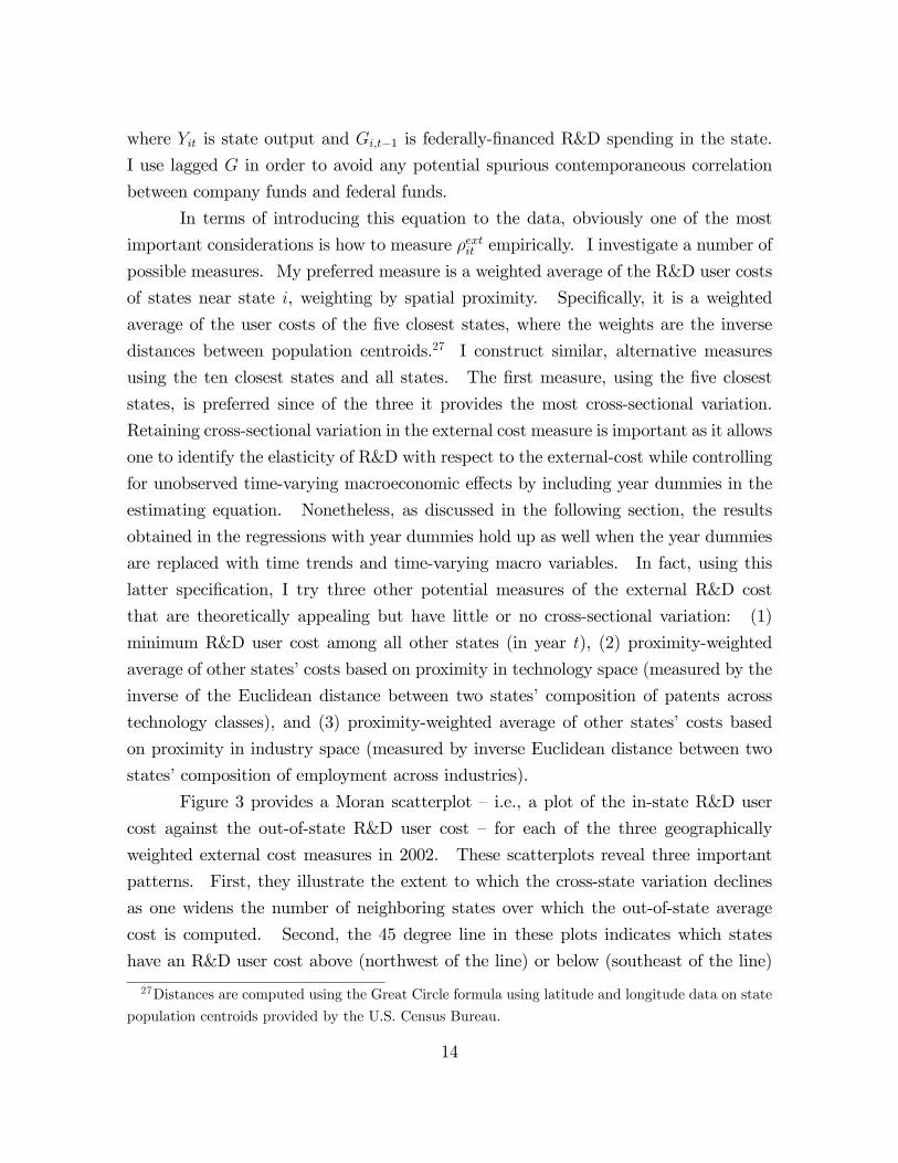
where Yit is state output and Gi;t�1 is federally-�nanced R&D spending in the state.
I use lagged G in order to avoid any potential spurious contemporaneous correlation
between company funds and federal funds.
In terms of introducing this equation to the data, obviously one of the most
important considerations is how to measure �extit empirically. I investigate a number of
possible measures. My preferred measure is a weighted average of the R&D user costs
of states near state i, weighting by spatial proximity. Speci�cally, it is a weighted
average of the user costs of the �ve closest states, where the weights are the inverse
distances between population centroids.27 I construct similar, alternative measures
using the ten closest states and all states. The �rst measure, using the �ve closest
states, is preferred since of the three it provides the most cross-sectional variation.
Retaining cross-sectional variation in the external cost measure is important as it allows
one to identify the elasticity of R&D with respect to the external-cost while controlling
for unobserved time-varying macroeconomic e¤ects by including year dummies in the
estimating equation. Nonetheless, as discussed in the following section, the results
obtained in the regressions with year dummies hold up as well when the year dummies
are replaced with time trends and time-varying macro variables. In fact, using this
latter speci�cation, I try three other potential measures of the external R&D cost
that are theoretically appealing but have little or no cross-sectional variation: (1)
minimum R&D user cost among all other states (in year t), (2) proximity-weighted
average of other states�costs based on proximity in technology space (measured by the
inverse of the Euclidean distance between two states�composition of patents across
technology classes), and (3) proximity-weighted average of other states� costs based
on proximity in industry space (measured by inverse Euclidean distance between two
states�composition of employment across industries).
Figure 3 provides a Moran scatterplot � i.e., a plot of the in-state R&D user
cost against the out-of-state R&D user cost � for each of the three geographically
weighted external cost measures in 2002. These scatterplots reveal three important
patterns. First, they illustrate the extent to which the cross-state variation declines
as one widens the number of neighboring states over which the out-of-state average
cost is computed. Second, the 45 degree line in these plots indicates which states
have an R&D user cost above (northwest of the line) or below (southeast of the line)
27Distances are computed using the Great Circle formula using latitude and longitude data on state
population centroids provided by the U.S. Census Bureau.
14
the average cost of their neighbors. For example, states like Hawaii, Rhode Island,
Georgia, New Jersey, and West Virginia have in-state R&D costs that are considerably
lower than the average cost of their neighboring states. The third and perhaps most
interesting pattern revealed in Figure 3 is that there is a clear positive correlation
between a state�s own R&D cost and the average cost of its near neighbors. This
pattern is revealed most clearly in the top-left panel, where the out-of-state cost is
the weighted average among the �ve closest states. Note, for instance, that all of
the mid-Atlantic states �Virginia, Maryland, D.C., Delaware, and Pennsylvania �are
found in the upper-right region of the plot, while Paci�c West and New England states
tend to be found in the lower-left region. The correlation coe¢ cient is 0:23 (p-value
= 0:10). Though further analysis, beyond the scope of this paper, would be required
to fully assess this relationship, the strong positive correlation is at least suggestive of
a strategic interaction between lawmakers in one state and lawmakers in nearby states
when it comes to choosing R&D tax incentives. Such a positively-sloping reaction
function is a necessary prerequisite for a so-called �race to the bottom�among states
that many policymakers have argued has been happening in recent years with regard
to R&D credits and other business tax incentives.
It should also be noted that, theoretically, the R&D input(s) into the production
function are R&D capital services, which are unobserved. There are two possible ways
to proxy for unobserved capital services. One can assume that the �ow of R&D capital
services in a year is proportional to either R&D investment in that year or the R&D
capital stock in that year. Given the inherent di¢ culty in measuring the depreciation
rate of the R&D stock and the fact that even-year data is missing prior to 1997, I opt to
use R&D investment instead, as is commonly done in the literature. As a robustness
check, though, I also report results below based on an R&D stock constructed using the
perpetual inventory method assuming a 15% depreciation rate and �lling in even-year
investment data via interpolation between adjacent years.
3.2 Dynamic Model
The above factor demand model assumes that there are no adjustment costs/frictions
associated with R&D capital. There is, however, ample evidence that �rms face high
adjustment costs relating to R&D (Bernstein and Nadiri [1986]; Hall, Griliches, and
Hausman [1986]; Hall and Hayashi [1988]; Himmelberg and Petersen [1990]; and Hall
[1993b]). Not only may there be substantial costs involved with large year-to-year15
changes in R&D spending for a given R&D facility, but there also may be substantial
costs associated with moving R&D activity from one state to another. Note that for a
�rm in one state to take advantage of another state�s reduction in the R&D user cost,
the �rm must not only conduct its R&D in the latter state but must also generate
income in that state, another potential cost of adjusting locations. All of these cost
imply that in each period �rms will only partially adjust R&D to their desired levels.
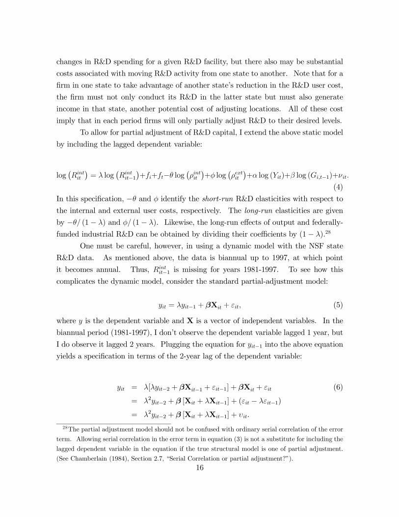
To allow for partial adjustment of R&D capital, I extend the above static model
by including the lagged dependent variable:
log�Rintit
�= � log
�Rintit�1
�+fi+ft�� log
��intit�+� log
��extit
�+� log (Yit)+� log (Gi;t�1)+�it:
(4)
In this speci�cation, �� and � identify the short-run R&D elasticities with respect tothe internal and external user costs, respectively. The long-run elasticities are given
by ��= (1� �) and �= (1� �). Likewise, the long-run e¤ects of output and federally-funded industrial R&D can be obtained by dividing their coe¢ cients by (1� �).28
One must be careful, however, in using a dynamic model with the NSF state
R&D data. As mentioned above, the data is biannual up to 1997, at which point
it becomes annual. Thus, Rintit�1 is missing for years 1981-1997. To see how this
complicates the dynamic model, consider the standard partial-adjustment model:
yit = �yit�1 + �Xit + "it; (5)
where y is the dependent variable and X is a vector of independent variables. In the
biannual period (1981-1997), I don�t observe the dependent variable lagged 1 year, but
I do observe it lagged 2 years. Plugging the equation for yit�1 into the above equation
yields a speci�cation in terms of the 2-year lag of the dependent variable:
yit = �[�yit�2 + �Xit�1 + "it�1] + �Xit + "it (6)
= �2yit�2 + � [Xit + �Xit�1] + ("it � �"it�1)= �2yit�2 + � [Xit + �Xit�1] + �it.
28The partial adjustment model should not be confused with ordinary serial correlation of the error
term. Allowing serial correlation in the error term in equation (3) is not a substitute for including the
lagged dependent variable in the equation if the true structural model is one of partial adjustment.
(See Chamberlain (1984), Section 2.7, �Serial Correlation or partial adjustment?�).
16
In our context, this equation would express current R&D as a function of R&D lagged
2 years, and current and lagged values of the independent variables. Since all of the
independent variables in X except G (which, like R, is biannual until 1997) are ob-
served annually, this equation can be estimated directly using a non-linear estimator.29
I perform such an estimation using non-linear least squares (NLLS) after imputing
missing G data based on adjacent years and obtain (and present below) results similar
to the results from the linear estimation I describe next. The results presented in
Section 4, however, will focus on the linear estimation as it does not rely on imputed
data (for G).
If Xit�1 is uncorrelated with Xit, one can obtain consistent estimates of � and
� using a linear estimator such as generalized least squares (GLS) and omitting the
unobserved Xit�1 variables. In this case, the proper model is yit = �2yit�2+�Xit+�it
for t � 1997 and yit = �yit�1 + �Xit + "it for t > 1997. These two equations can
be estimated simultaneously by simply pooling the biannual and annual samples but
allowing the coe¢ cient on the lagged dependent variable, � or �2, to vary across the
two periods (while constraining � to be equal over the entire sample). This is the
main estimation strategy employed in this paper.
Of course, if the lagged values of the independent variables have an e¤ect on
current R&D (independent of the e¤ect from the current values of the independent
variables), and the independent variables are autocorrelated, then the GLS within
estimator will be biased away from zero. However, since the e¤ects of lagged values
is likely to be swamped by the e¤ects of current values, this bias is likely to be small.
As shown in Section 4, this conjecture is supported by the fact that the � estimates
obtained via NLLS estimation of equation (6) match closely the GLS estimates of this
linear speci�cation.
3.3 Estimation Strategy
The identi�cation of can be obtained with the conventional di¤erence-in-di¤erences
(DID) estimator. In the present panel data context with state �xed e¤ects, the DID
estimator is equivalent to the within-groups (or simply �within�) estimator. Under the
29The error �it will be AR(1) within state and may be heteroskedastic. I therefore estimate
the above equation using a VC matrix that is heteroskedasticity-consistent (Hausman-White VC
estimator) and allows for �rst-order autocorrelation of errors within-state. It is assumed that both
Xit�1 and Xit are orthogonal to �it.
17
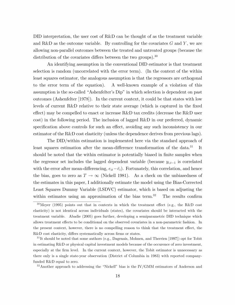
DID interpretation, the user cost of R&D can be thought of as the treatment variable
and R&D as the outcome variable. By controlling for the covariates G and Y , we are
allowing non-parallel outcomes between the treated and untreated groups (because the
distribution of the covariates di¤ers between the two groups).30
An identifying assumption in the conventional DID estimator is that treatment
selection is random (uncorrelated with the error term). (In the context of the within
least squares estimator, the analogous assumption is that the regressors are orthogonal
to the error term of the equation). A well-known example of a violation of this
assumption is the so-called �Ashenfelter�s Dip�in which selection is dependent on past
outcomes (Ashenfelter [1978]). In the current context, it could be that states with low
levels of current R&D relative to their state average (which is captured in the �xed
e¤ect) may be compelled to enact or increase R&D tax credits (decrease the R&D user
cost) in the following period. The inclusion of lagged R&D in our preferred, dynamic
speci�cation above controls for such an e¤ect, avoiding any such inconsistency in our
estimator of the R&D cost elasticity (unless the dependence derives from previous lags).
The DID/within estimation is implemented here via the standard approach of
least squares estimation after the mean-di¤erence transformation of the data.31 It
should be noted that the within estimator is potentially biased in �nite samples when
the regressor set includes the lagged dependent variable (because yi;t�1 is correlated
with the error after mean-di¤erencing, eit��ei). Fortunately, this correlation, and hencethe bias, goes to zero as T ! 1 (Nickell 1981). As a check on the unbiasedness of
the estimates in this paper, I additionally estimate the model using the Bias-Corrected
Least Squares Dummy Variable (LSDVC) estimator, which is based on adjusting the
within estimates using an approximation of the bias term.32 The results con�rm
30Meyer (1995) points out that in contexts in which the treatment e¤ect (e.g., the R&D cost
elasticity) is not identical across individuals (states), the covariates should be interacted with the
treatment variable. Abadie (2005) goes further, developing a semiparametric DID technique which
allows treatment e¤ects to be conditional on the observed covariates in a non-parametric fashion. In
the present context, however, there is no compelling reason to think that the treatment e¤ect, the
R&D cost elasticity, di¤ers systematically across �rms or states.31It should be noted that some authors (e.g., Dagenais, Mohnen, and Therrien [1997]) opt for Tobit
in estimating R&D or physical capital investment models because of the occurence of zero investment,
especially at the �rm level. In the current context, however, the Tobit estimator is unnecessary as
there only is a single state-year observation (District of Columbia in 1983) with reported company-
funded R&D equal to zero.32Another approach to addressing the �Nickell�bias is the IV/GMM estimators of Anderson and
18
that the original estimates are approximately unbiased (LSDVC results available upon
request).33
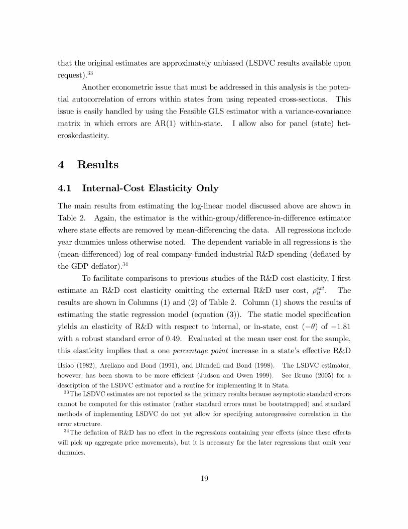
Another econometric issue that must be addressed in this analysis is the poten-
tial autocorrelation of errors within states from using repeated cross-sections. This
issue is easily handled by using the Feasible GLS estimator with a variance-covariance
matrix in which errors are AR(1) within-state. I allow also for panel (state) het-
eroskedasticity.
4 Results
4.1 Internal-Cost Elasticity Only
The main results from estimating the log-linear model discussed above are shown in
Table 2. Again, the estimator is the within-group/di¤erence-in-di¤erence estimator
where state e¤ects are removed by mean-di¤erencing the data. All regressions include
year dummies unless otherwise noted. The dependent variable in all regressions is the
(mean-di¤erenced) log of real company-funded industrial R&D spending (de�ated by
the GDP de�ator).34
To facilitate comparisons to previous studies of the R&D cost elasticity, I �rst
estimate an R&D cost elasticity omitting the external R&D user cost, �extit . The
results are shown in Columns (1) and (2) of Table 2. Column (1) shows the results of
estimating the static regression model (equation (3)). The static model speci�cation
yields an elasticity of R&D with respect to internal, or in-state, cost (��) of �1:81with a robust standard error of 0:49. Evaluated at the mean user cost for the sample,
this elasticity implies that a one percentage point increase in a state�s e¤ective R&D
Hsiao (1982), Arellano and Bond (1991), and Blundell and Bond (1998). The LSDVC estimator,
however, has been shown to be more e¢ cient (Judson and Owen 1999). See Bruno (2005) for a
description of the LSDVC estimator and a routine for implementing it in Stata.33The LSDVC estimates are not reported as the primary results because asymptotic standard errors
cannot be computed for this estimator (rather standard errors must be bootstrapped) and standard
methods of implementing LSDVC do not yet allow for specifying autoregressive correlation in the
error structure.34The de�ation of R&D has no e¤ect in the regressions containing year e¤ects (since these e¤ects
will pick up aggregate price movements), but it is necessary for the later regressions that omit year
dummies.
19
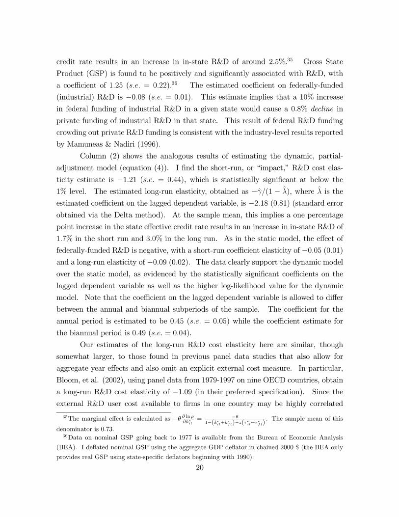
credit rate results in an increase in in-state R&D of around 2:5%.35 Gross State
Product (GSP) is found to be positively and signi�cantly associated with R&D, with
a coe¢ cient of 1:25 (s:e: = 0:22).36 The estimated coe¢ cient on federally-funded
(industrial) R&D is �0:08 (s:e: = 0:01). This estimate implies that a 10% increase
in federal funding of industrial R&D in a given state would cause a 0:8% decline in
private funding of industrial R&D in that state. This result of federal R&D funding
crowding out private R&D funding is consistent with the industry-level results reported
by Mamuneas & Nadiri (1996).
Column (2) shows the analogous results of estimating the dynamic, partial-
adjustment model (equation (4)). I �nd the short-run, or �impact,�R&D cost elas-
ticity estimate is �1:21 (s:e: = 0:44), which is statistically signi�cant at below the
1% level. The estimated long-run elasticity, obtained as � ̂=(1 � �̂), where �̂ is theestimated coe¢ cient on the lagged dependent variable, is �2:18 (0:81) (standard errorobtained via the Delta method). At the sample mean, this implies a one percentage
point increase in the state e¤ective credit rate results in an increase in in-state R&D of
1:7% in the short run and 3:0% in the long run. As in the static model, the e¤ect of
federally-funded R&D is negative, with a short-run coe¢ cient elasticity of �0:05 (0:01)and a long-run elasticity of �0:09 (0:02). The data clearly support the dynamic modelover the static model, as evidenced by the statistically signi�cant coe¢ cients on the
lagged dependent variable as well as the higher log-likelihood value for the dynamic
model. Note that the coe¢ cient on the lagged dependent variable is allowed to di¤er
between the annual and biannual subperiods of the sample. The coe¢ cient for the
annual period is estimated to be 0:45 (s:e: = 0:05) while the coe¢ cient estimate for
the biannual period is 0:49 (s:e: = 0:04).
Our estimates of the long-run R&D cost elasticity here are similar, though
somewhat larger, to those found in previous panel data studies that also allow for
aggregate year e¤ects and also omit an explicit external cost measure. In particular,
Bloom, et al. (2002), using panel data from 1979-1997 on nine OECD countries, obtain
a long-run R&D cost elasticity of �1:09 (in their preferred speci�cation). Since the
external R&D user cost available to �rms in one country may be highly correlated
35The marginal e¤ect is calculated as �� @ ln �@keit= ��
1�(keit+keft)�z(�eit+�eft). The sample mean of this
denominator is 0:73.36Data on nominal GSP going back to 1977 is available from the Bureau of Economic Analysis
(BEA). I de�ated nominal GSP using the aggregate GDP de�ator in chained 2000 $ (the BEA only
provides real GSP using state-speci�c de�ators beginning with 1990).
20
to that available to �rms in other countries, the e¤ect of the external R&D user cost
likely will be picked up to a large extent in their year e¤ects. Thus, I would argue
that the elasticity estimate from that study should be treated as an unbiased estimate
of the internal (domestic) R&D cost elasticity but may not necessarily be equal to the
aggregate R&D cost elasticity (though �rms are likely far less mobile across countries
than across states). As I show in the next subsection, explicitly accounting for external
R&D costs results in an aggregate R&D cost elasticity that is far smaller than the
internal R&D cost elasticity, at least at the level of U.S. states.
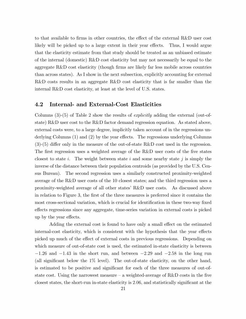
4.2 Internal- and External-Cost Elasticities
Columns (3)-(5) of Table 2 show the results of explicitly adding the external (out-of-
state) R&D user cost to the R&D factor demand regression equation. As stated above,
external costs were, to a large degree, implicitly taken account of in the regressions un-
derlying Columns (1) and (2) by the year e¤ects. The regressions underlying Columns
(3)-(5) di¤er only in the measure of the out-of-state R&D cost used in the regression.
The �rst regression uses a weighted average of the R&D user costs of the �ve states
closest to state i. The weight between state i and some nearby state j is simply the
inverse of the distance between their population centroids (as provided by the U.S. Cen-
sus Bureau). The second regression uses a similarly constructed proximity-weighted
average of the R&D user costs of the 10 closest states; and the third regression uses a
proximity-weighted average of all other states�R&D user costs. As discussed above
in relation to Figure 3, the �rst of the three measures is preferred since it contains the
most cross-sectional variation, which is crucial for identi�cation in these two-way �xed
e¤ects regressions since any aggregate, time-series variation in external costs is picked
up by the year e¤ects.
Adding the external cost is found to have only a small e¤ect on the estimated
internal-cost elasticity, which is consistent with the hypothesis that the year e¤ects
picked up much of the e¤ect of external costs in previous regressions. Depending on
which measure of out-of-state cost is used, the estimated in-state elasticity is between
�1:26 and �1:43 in the short run, and between �2:29 and �2:58 in the long run(all signi�cant below the 1% level). The out-of-state elasticity, on the other hand,
is estimated to be positive and signi�cant for each of the three measures of out-of-
state cost. Using the narrowest measure �a weighted-average of R&D costs in the �ve
closest states, the short-run in-state elasticity is 2:06, and statistically signi�cant at the21
5% level. The implied long-run in-state elasticity is 3:72. The implied aggregate-cost
elasticity �the sum of the in-state and out-of-state elasticities �is relatively small and
statistically insigni�cant.
As one broadens the measure of out-of-state cost by including more outside
states in the weighted average, which reduces cross-sectional variation, the out-of-state
elasticity estimate becomes increasingly imprecise. Nonetheless, even with the broader
out-of-state cost measures used in the regressions underlying columns (3) and (4), the
elasticity is found to be positive and signi�cant at below the 5% level, and in no case
is the aggregate-cost elasticity found to be signi�cantly di¤erent from zero.37
Table 3 provides estimates based on analogous regressions to those underlying
Columns (3)-(5) but replacing the year dummies with a year trend and GDP to capture
aggregate macroeconomic shocks to R&D spending.38 I also separately included log(rt+
�) even though this term is already part of log (�init ) and log (�outit ) to allow for possible
endogeneity of the real interest rate. (Note log(rt+�) is absorbed by the year e¤ects in
the previous regressions.) The estimated elasticities are qualitatively similar to those
in Table 2, but are estimated here with much greater precision. Similar to the Table 2
results, the internal-cost elasticity is around �1:5 (in the short run) while the external-cost elasticity is around +1:6. The long-run internal and external elasticities are
somewhat higher, at around �2:5 and +2:8, respectively. Both in the short run and
in the long run, the implied aggregate-cost elasticity is essentially zero (and precisely
estimated). The results are quite consistent across the three measures of external cost.
The estimated coe¢ cients on the other variables are virtually unchanged from
the previous, two-way �xed-e¤ects regressions. The elasticity of private R&D with
respect to federal R&D funding is precisely estimated at �0:06. The coe¢ cient on
GSP is just slightly higher, at about 0:7, than found in the previous regressions. In-
terestingly, I �nd that holding a state�s own gross product constant, the gross product
of the rest of the nation (i.e., GDP) has a negative and signi�cant e¤ect on state R&D
spending, with an elasticity around �0:9. This suggests that as with costs, what mat-ters for a state�s R&D demand is not the absolute size of its economy but rather its size
37This �nding of a near-zero aggregate-cost elasticity is consistent with Bloom and Gri¢ th (2001)
who perform related regressions using cross-country panel data and also �nd an aggregate R&D
elasticity that is insigni�cantly di¤erent from zero (though the elasticities are estimated with far less
precision than are those in this paper).38Unreported regressions including either a quadratic time trend or presidential-term dummies
yielded similar results.
22
relative to the rest of the nation. That is, it appears that R&D activity may relocate
out of state not just in response to favorable changes in out-of-state R&D costs, but
also in response to comparatively faster economic growth outside of the state.
4.3 Robustness Checks
In this subsection, I describe three checks on the robustness of the results described
above. The �rst check involves using alternative measures, unrelated to geographic dis-
tance, of the out-of-state R&D user cost. The second check veri�es that the estimates
in Tables 2 and 3 are not biased due to the omission of even-year data between 1981-
1997. I verify this by estimating the non-linear partial-adjustment model shown in
equation (6) via non-linear least squares (NLLS). The third robustness check consists
of replacing the �ow (investment) of R&D as the dependent variable with an imputed
measure of the stock of R&D. A number of additional exercises, not shown here, also
con�rm the robustness of these regressions (results available upon request). These
robustnesss checks include: including additional out-of-state factors (constructed as
above) such as out-of-state GDP and population, allowing for potential R&D data-
reporting/selection bias via a Heckman two-step estimator, and excluding Alaska and
Hawaii from the sample.
Table 4 shows the results of using yet three other possible measures of the out-
of-state R&D user cost in the one-way �xed e¤ects speci�cation. The �rst measure,
used in the regression underlying Column (1), is the best, i.e., lowest, R&D user cost
available in a given year (among all states). If relocation costs are independent of
distance (along geographical, technological, industrial, or any other dimension), then
the minimum-cost state will be the relevant alternative location considered by �rms
in other states when deciding where and how much R&D to conduct. Column (2) of
Table 4 shows the results from measuring the out-of-state cost as a technology-based
weighted average of other states�costs, where the weight between state i and each other
state is the inverse of the Euclidean distance between the two states�composition of
patents across technology classes39. This measure is appropriate if �rms focus dispro-
portionately on states with other �rms in similar technological �elds when considering
alternative R&D locations. The third external-cost measure (Column (3)) is analo-
gous but weights other states R&D costs according to the inverse Euclidean distance
39The annual number of patent grants in each state in each of 401 technology classes is provided by
the U.S. Patent and Trademark O¢ ce.
23
between state i�s and each other state�s composition of employment across industries.40
Though these alternative measures yield di¤erent estimates for the internal-
cost elasticity, compared with each other or with the elasticities from Table 3, they
all yield an aggregate-cost elasticity that is, again, very close to zero (and statistically
insigni�cant). The minimum-cost measure yields the lowest and least statistically
signi�cant estimates for the (short-run) internal- and external cost elasticities, at about
�0:67 and 0:78, respectively. The other technology and industry based measures yieldestimates very similar to those using the distance-based measures of external costs.
Using the technology-based measure results in short-run cost elasticities of �1:2 and1:4, respectively, for the internal- and external-cost elasticities. Recall that the cost
elasticities estimated using the distance-based measure (Table 3) were about �1:5 and1:6, respectively. The industry-based measure yields similar, though slightly smaller,
elasticities at about �1:1 and 1:3. As for the other explanatory variables, using thesealternative external-cost measures has very little e¤ect on their coe¢ cient estimates.
As discussed in Section 3.2 above, because of the biannual nature of the R&D
data before 1997, the log-linear speci�cation used thus far will provide consistent es-
timates only if the explanatory variables are independent of their (omitted) lagged
values. Here I assess whether this identi�cation assumption a¤ects the estimates in
any quantitatively important way by estimating the non-linear speci�cation discussed
earlier (equation (6)), which is robust to serial correlation in the explanatory variables.
This speci�cation allows one to use the even-year data available on the independent
variables even though even-year data on the dependent variable, R&D, is unobserved.41
Speci�cally, the estimating equation becomes:
log(Rintit ) = �2 log(Rintit�2) + fi + ft � � log(�intit )� �� log(�intit�1) + � log(�extit ) + �� log(�extit�1)+� log (Yit) + �� log (Yit�1) + � log (Gi;t�1) + �� log (Gi;t�2) + �it,
where f ; �; �g are impact coe¢ cients. The long-run e¤ects are found by dividing thecoe¢ cients by (1� �).40For each year, I compute employment shares for all states that have non-missing company R&D
data using the lowest common level of industry aggregation possible for this set of states. Therefore,
the level of aggregation is year-speci�c, but roughly-speaking, it matches the 3-digit SIC level. The
data comes from the BLS ES-202 database.41Even-year data is available for all explanatory variables except federally-funded R&D spending.
I impute even-year data for this variable by interpolating between adjacent years.
24
I estimate this equation via non-linear least squares (NLLS). Table 5 reports
the results from estimating the non-linear analogs to the three linear regressions of
primary concern from above, namely the regressions underlying Columns (2) and (3)
of Table 2 and Column 1 of Table 3. The �rst of these regressions includes federal
R&D, GSP, the internal R&D user cost, and twice-lagged company R&D. The second
includes these variables plus the external user cost (measured using the proximity-
weighted average of the �ve closest states). The third replaces year e¤ects with GDP
and a year trend.
The estimated R&D cost elasticities obtained from the non-linear model are
similar to those obtained via the linear model, though the standard errors are higher.
As with the linear model, the non-linear model yields an aggregate-cost elasticity that is
considerably smaller than that estimated by previous studies and statistically insignif-
icant from zero. Thus, the non-linear estimation con�rms the linear model�s results
that (1) the internal cost elasticity is negative and above unity (in absolute value),
(2) the external cost elasticity is positive and above unity, and (3) the aggregate-cost
elasticity is small and not signi�cantly di¤erent from zero.42
As a �nal robustness check, I experiment with using a measure of the R&D stock
rather than the R&D investment �ow for the dependent variable in the regressions. I
construct a measure of the R&D stock via a perpetual inventory of past investment
assuming a depreciation rate of 15%. I �rst �ll in missing years of R&D investment
data via interpolation between adjacent years with non-missing data. If a state is
missing more than 3 consecutive years of data, I drop these state-years from the sample
beginning in the �rst year of missing data.
There are three main drawbacks to using the R&D stock data instead of R&D
investment data (and hence why I use the investment data for the main results of the
paper). First, there is substantial uncertainty regarding the true depreciation rate.
Second, computing the stock entails using interpolated data. Third, the R&D stock
is very autocorrelated: In regressions based on the dynamic model using the stock,
the coe¢ cient on the (annual) lagged dependent variable generally is 0:75 or higher.
This autocorrelation makes it di¢ cult to accurately estimate the long-run e¤ect of a
given variable. With those caveats in mind, estimating the preferred speci�cation
42One di¤erence between the non-linear and linear results worth mentioning is that the coe¢ cient
on federally-funded R&D is closer to zero and insigni�cant in the non-linear regressions. This is likely
due to attenuation bias resulting from the imputation of even-year data for this variable.
25
(that in Column 1 of Table 3) using the (mean-di¤erenced log) R&D stock measure
as the dependent variable yields qualitatively similar results to those using R&D �ow.
The estimated short-run internal-cost elasticity is �0:24 (s:e: = 0:16) and the external-cost elasticity is 0:41 (0:17).43 The implied long-run elasticities are, respectively, �0:99(0:66) and 1:67 (0:71). The implied aggregate-cost elasticity is 0:17 (0:07) in the short-
run and 0:68 (0:31) in the long-run. In sum, using a measure of R&D stock instead
of the R&D �ow, the data still point toward a negative and signi�cant internal-cost
elasticity, a positive and signi�cant external-cost elasticity, and a small and insigni�cant
(though imprecisely estimated) aggregate-cost elasticity.
4.4 Comparison to previous studies
Table 6 summarizes the results of previous studies that estimate the R&D cost elastic-
ity. In the last row of the table, I include the estimated internal-cost elasticity from
this paper based on the speci�cations that do not explicitly include the external user
cost (though these speci�cations implicitly include the external user cost because they
include year e¤ects). Focusing on the more recent studies �in particular, those using
post-1981 data (i.e., after the introduction of the U.S. federal R&D tax credit) �one
can see that the internal-cost estimates in this paper are at the upper end of the range
of those found previously.
Hines (1993) performs a �rm-level panel data estimation over the 1984-89 pe-
riod, relying on the cross-�rm variation in the tax treatment of R&D for certain U.S.
multinational �rms. He estimates a short-run R&D cost elasticity of between �1:2and �1:6, and a long-run elasticity between �1:3 and �2:0. Hall (1993a) obtains sim-ilar estimates: a short-run elasticity of �0:84 to �1:5 and a long-run elasticity of �2:0to �2:7. Hall relies on cross-�rm variation in tax positions for publicly-traded �rms
between 1981 and 1991. Bloom, et al. (2002), in their preferred dynamic speci�ca-
tion, �nd a short-run elasticity of �0:14 and a long-run elasticity of �1:09 using across-country panel over the 1979-1997 period. None of these three studies control for
the potential e¤ect of federally-funded R&D on private R&D. Mamuneas and Nadiri
(1996) estimate a cost function containing the after-tax price of company-funded R&D,
prices of other inputs, and the stock of federally-funded R&D (both within-industry
and external to industry). They use data from 1956-88 for 12 manufacturing industries.
43The full set of results from this regression are available from the author upon request.
26
The variation in the R&D price in their study comes from the fact that industries have
di¤erent R&D input mixes and therefore di¤erent R&D economic depreciation rates.
They obtain industry-speci�c estimates of the (short-run) R&D price elasticity ranging
from �0:94 to �1. As in this paper, their estimates of cross-price elasticities suggestthat company-funded and federally-funded R&D are substitutes.
All of these previous studies ignore state-level R&D tax credits in their calcu-
lations of the overall R&D tax price, though this is less problematic for the studies
using earlier sample periods since state R&D tax credits became quantitatively more
important over time. The resulting mismeasurement of the true extent of R&D tax
incentives could lead to overestimation of the R&D spending response to R&D tax
credits.
It is illuminating also to compare the R&D cost elasticity estimates to esti-
mates in the literature of the user cost elasticity of physical capital. Interestingly,
recent econometric studies of the (long-run) physical user cost elasticity have obtained
estimates that are quite small, similar to the near-zero aggregate-cost elasticity esti-
mates obtained in this paper. Chirinko, et al. (1999) �nd an elasticity of �0:25. Theyalso show that the elasticity implied by results from Cummins, Hassett, and Hubbard
(1994) is �0:16, and that implied by Cummins and Hassett (1992) is �0:23 for equip-ment and �0:07 for structures. These results from the physical capital literature showthat the �nding in this paper of a small, near-zero aggregate R&D cost elasticity is not
implausible; in fact it is quite consistent with the �ndings regarding physical capital�s
cost elasticity.
5 Policy Implications and Conclusions
This paper o¤ers two important new �ndings to the literature. First, I �nd that the
R&D spending in a state is negatively impacted by R&D tax incentives in other states,
presumably as �rms shift R&D spending to the state or states with cheaper R&D user
costs. Second, the magnitude of this response (i.e., the elasticity) is nearly as large
as the response to an increase in a state�s own user cost. Each of these �ndings have
very important policy implications.
The �rst �nding indicates that a state�s R&D �scal policies impose an exter-
nality on R&D activity, and its associated bene�ts, in other states. Given recent U.S.
federal court rulings, this �nding raises interesting questions regarding the constitu-
27
tionality of state R&D tax credits (see Wilson [2005] for a discussion). Speci�cally,
in the recent case Cuno v. DaimlerChrysler, et al. (2004), the Sixth Circuit Court of
Appeals, citing a number of Supreme Court rulings, invalidated an Ohio investment
tax credit on the grounds that it violated what is known as the �dormant Commerce
Clause.� This dormant clause of the U.S. Constitution holds that only Congress has
the power to regulate interstate commerce and thus certain limits apply to a state�s
ability to adopt tax policies that a¤ect commerce in other states. The Supreme Court
has established that a tax violates this clause if it di¤erentially, or �discriminatorily,�
�tax[es] the products manufactured or the business operations in any other State�
(Boston Stock Exchange v. State Tax Commission [1977]). The Court has further
stated that the fact that a tax statute discriminates against operations in other states
via a tax credit instead of a tax is irrelevant (both legally and economically). In the
Cuno decision, the Sixth Circuit Court of Appeals stated that the determination of
whether a tax or credit is discriminatory should be decided �on the basis of �a sensitive,
case-by-case analysis of purposes and e¤ects,�...�into whether �the provision �will in its
practical operation work discrimination against interstate commerce,..., by providing
a direct commercial advantage to local business.�� (Cuno v. DaimlerChrysler, citing
Supreme Court decisions West Lynn Creamery v. Healy [1994] and Bacchus Imports
v. Dias [1984]). Similar cases currently are pending in a number of states. Thus,
analyses into the e¤ect of outside states�R&D tax credits into the R&D activity of a
given state, such as the analysis done in this paper, are critical to the issue of whether
state R&D tax credits are constitutional. The �ndings of this paper suggest that state
R&D tax credits may in fact be discriminatory both in statute and in practice.
The second major �nding of this paper �that the internal and external user
cost elasticities are of opposite signs and roughly equal magnitudes �suggests nearly
costless geographic mobility in R&D activity. It also implies that the aggregate R&D
cost elasticity �the R&D cost elasticity that is relevant for social welfare cost-bene�t
analyses of R&D tax credits � is actually quite small, suggesting that the setting of
R&D tax credits by states (as opposed to only the federal government) is nearly a
zero-sum game. For instance, if all states were to lower their R&D user costs, e.g., by
raising their tax credit rates, by the same percentage, aggregate private R&D in the
nation would rise very little, if at all.
What these �ndings imply regarding the e¤ectiveness of the U.S. federal R&D
tax credit depends on the degree of international mobility of R&D. In the current
28
era of globalization, it seems likely that large foreign and U.S. multinationals, which
are responsible for the bulk of U.S. R&D spending, may fairly easily reallocate R&D
activity to (from) the U.S. in response to favorable (unfavorable) changes in U.S. policy
viz-a-viz foreign policy. Thus, the degree of international R&D mobility remains an
important topic for future research.
6 References
References
[1] Abadie, Alberto. "Semiparametric Di¤erence-in-Di¤erences Estimators." Review
of Economic Studies 72, no. 1 (2005): 1-19.
[2] Anderson, T. W., and C. Hsiao. "Formulation and Estimation of Dynamic Models
Using Panel Data." Journal of Econometrics, 1982.
[3] Arellano, Manuel, and Stephen R. Bond. "Some Tests of Speci�cation for Panel
Data: Monte Carlo Evidence and Application to Employment Equations." Review
of Economic Studies, 1991.
[4] Ashenfelter, Orley. "Estimating the E¤ect of Training Programs on Earnings."
Review of Economics and Statistics 60 (1978): 47-57.
[5] Baily, Martin, and Robert Z. Lawrence. �Tax Incentives for R&D: What Do the
Data Tell Us?�Study commissioned by the Council on Research and Technology,
Washington, D.C.. September 1995.
[6] Beaulieu, Eugene, Kenneth J. McKenzie, and Jean-François Wen. "Do Taxes Mat-
ter for Firm Location? Evidence From Canadian Provinces." Mimeo, U. of Cal-
gary, 2004.
[7] Berger, Philip G. "Explicit and Implicit Tax E¤ects of the R & D Tax Credit."
Journal of Accounting Research 31, no. 2 (1993).
[8] Bernstein, Je¤rey L., andM. Ishaq Nadiri. "Financing and Investment in Plant and
Equipment and Research and Development"." Prices, Competition, and Equilib-
rium. Editors M. H. Pesaran and R. E. Quandt. Oxford: Philip Allan, 1986,233-48.
29
[9] Bloom, Nick, and Rachel Gri¢ th. "The Internationalisation of UK R&D." Fiscal
Studies 22, no. 3 (2001): 337-55.
[10] Bloom, Nick, Rachel Gri¢ th, and John Van Reenen. "Do R&D Tax Credits Work?
Evidence From a Panel of Countries 1979-97 ." Journal of Public Economics 85,
no. 1 (2002): 1-31.
[11] Blundell, Richard W., and Stephen R. Bond. "Initial Conditions and Moment
Restrictions in Dynamic Panel Data Models." Journal of Econometrics, 1998.
[12] The Book of the States. The Council of State Governments (Lexington, KY)
(Various Years).
[13] Bruno, Giovanni S. F. "Estimation and Inference in Dynamic Unbalanced Panel-
Data Models With a Small Number of Individuals." Stata Journal, 2005.
[14] Buss, Terry F. "The E¤ect of State Tax Incentives on Economic Growth and
Firm Location Decisions: An Overview of the Literature." Economic Development
Quarterly, 2001.
[15] Cameron, Gavin. "On the Measurement of Real R&D - Divisia Price Indices for
UK Business Enterprise R&D." Research Evaluation 6, no. 3 (1996): 215-19.
[16] Carlton, D. W. "Location and Employment Choices of New Firms: An Econo-
metric Model With Discrete and Continuous Endogenous Variables." Review of
Economics and Statistics, 1983.
[17] Chirinko, Robert S., Steven M. Fazzari, and Andrew P. Meyer. "How Responsive
Is Business Capital Formation to Its User Cost? An Exploration With Micro
Data." Journal of Public Economics 74 (1999): 53-80.
[18] Cummins, Jason G., and Kevin A. Hassett. "The E¤ects of Taxation on Invest-
ment: New Evidence From Firm Level Panel Data." National Tax Journal 45
(1992): 243-52.
[19] Cummins, Jason G., Kevin A. Hassett, and R. Glenn Hubbard. "A Reconsid-
eration of Investment Behavior Using Tax Reforms As Natural Experiments."
Brookings Papers on Economic Activity 2 (1994): 1-60.
30
[20] Cuno, et al. v. DaimlerChrysler, et al. No. 01-3960, U.S. 6th Circuit Court of
Appeals (2004).
[21] Dagenais, Marcel, Pierre Mohnen, and Pierre Therrien. "Do Canadian Firms Re-
spond to Fiscal Incentives to Research and Development?" CIRANO Working
Paper 97s-34 (1997).
[22] David, Paul A., Bronwyn H. Hall, and Andrew A. Toole. �Is public R&D a com-
plement or substitute for private R&D? A Review of the Econometric Evidence.�
Research Policy 29 (2000): 497-529.
[23] Devereux, Michael P., and Rachel Gri¢ th. "Taxes and the Location of Production:
Evidence From a Panel of U.S. Multinationals." Journal of Public Economics,
1998.
[24] Grubert, Harry, and John Mutti. "Do Taxes In�uence Where U.S. Corporations
Invest? " National Tax Journal, 2000.
[25] Hall, Bronwyn. "R&D Tax Policy During the 1980s: Success or Failure?" Tax
Policy and the Economy.Vol. 7. Cambridge and London: MIT Press, 1993a,1-35.
[26] Hall, Bronwyn. "Industrial Research During the 1980s: Did the Rate of Return
Fall?" Brookings Papers on Economic Activity, no. 2 (1993b): 289-343.
[27] Hall, Bronwyn, Zvi Griliches, and Jerry A. Hausman. "Patents and R and D: Is
There a Lag?" International Economic Review 27, no. 2 (1986): 265-83.
[28] Hall, Bronwyn, and Fumio Hayashi. "Research and Development As an Invest-
ment." NBER Working Paper, no. 2973 (1989).
[29] Hall, Bronwyn, and Marta Wosinka. "E¤ectiveness of the California R&D Tax
Credit."1999a.
[30] Hall, Bronwyn, and Marta Wosinka. "The California R&D Tax Credit: Descrip-
tion, History, and Economic Analysis."1999b.
[31] Hall, Robert E., and Dale W. Jorgenson. "Tax Policy and Investment Behavior."
American Economic Review 57 (1967): 391-414.
31
[32] Himmelberg, Charles P., and Bruce C. Peterson. "R&D and Internal Finance: A
Panel Study of Small Firms in High-Tech Industries." Review of Economics and
Statistics 76, no. 1 (1994): 38-51.
[33] Hines, James R. Jr. "On the Sensitivity of R&D to Delicate Tax Changes: The
Behavior of U.S. Multinationals in the 1980s." Studies in International Taxation.
Editors Alberto Giovanni, R. Glenn Hubbard, and Joel Slemrod. Chicago: Uni-
versity of Chicago Press, 1993,149-94.
[34] Jones, Charles I., and John C. Williams. "Too Much of a Good Thing? The
Economics of Investment in R&D." Journal of Economic Growth 5, no. 1 (2000):
65-85.
[35] Judson, R. A., and A. L. Owen. "Estimating Dynamic Panel Data Models: A
Guide for Macroeconomists." Economics Letters, 1999.
[36] Mamuneas, Theofanis P., and M. Ishaq Nadiri. "Public R&D Policies and Cost
Behavior of the US Manufacturing Industries." Journal of Public Economics 63,
no. 1 (1996): 57-81.
[37] McCutchen, William M. Jr. "Estimating the Impact of the R&D Tax Credit
on Strategic Groups in the Pharmaceutical Industry." Research Policy 22, no.
4 (1993).
[38] Meyer, Bruce D. "Natural and Quasi-Experiments in Economics." Journal of Busi-
ness and Economic Statistics 13, no. 2 (1995): 151-61.
[39] National Science Foundation, Division of Science Resources Statistics. �Research
and Development in Industry: 2001,�NSF 05-305, Project O¢ cer, Raymond M.
Wolfe (Arlington, VA 2005).
[40] Newman, Robert J., and Dennis H. Sullivan. "Econometric Analysis of Business
Tax Impacts on Industrial Location: What Do We Know, and How Do We Know
It?" Journal of Urban Economics 23 (1988): 215-34.
[41] Oates, Wallace A. Fiscal Federalism. New York, NY: Harcourt Brace. 1972.
[42] ÓhUallacháin, Brendán, and Mark A. Satterthwaite. "Sectoral Growth Patterns
at the Metropolitan Level: An Evaluation of Economic Development Incentives."
Journal of Urban Economics 31 (1992): 25-58.32
[43] Pa¤, Lolita A. "State-Level R&D Tax Credits: A Firm-Level Analysis." Topics in
Economic Analysis & Policy (forthcoming).
[44] Papke, Leslie E. "Subnational Taxation and Capital Mobility: Estimates of Tax-
Price Elasticities." National Tax Journal, 1987.
[45] Papke, Leslie E. "Interstate Business Tax Di¤erentials and New Firm Location:
Evidence From Panel Data." Journal of Public Economics, 1991.
[46] Plesko, George A., and Robert Tannenwald. "Measuring the Incentive E¤ects of
State Tax Policies Toward Capital Investment." FRB Boston Working Paper 01-4,
2001.
[47] Sigalla, Fiona, and Alan D. Viard. "Would a Research Tax Credit Be a Good
Investment for Texas?" Southwest Economy, Federal Reserve Bank of Dallas, no.
2 (1999): 1-7.
[48] Signi�cant Features of Fiscal Federalism, American Council on Intergovernmental
A¤airs (Orange Grove, NJ) (Various Years).
[49] State Science and Technology Institute (SSTI). "State Research and Development
Tax Incentives."1997.
[50] Stark, Kirk and Daniel J. Wilson �What Do We Know about the Interstate Eco-
nomic E¤ects of State Tax Incentives?,�Georgetown Journal of Law and Public
Policy IV (1), 2006.
[51] State Tax Handbook, Commerce Clearing House, Inc. (Chicago, IL) (Various
Years).
[52] Swenson, C. W. "Some Tests of the Incentive E¤ects of the Research and Experi-
mentation Tax Credit." Journal of Public Economics 49, no. 2 (1992): 203-18.
[53] Tiebout, Charles M. "A Pure Theory of Local Expenditures." Journal of Political
Economy, 1956.
[54] Wheeler, David, and Ashoka Mody. "International Investment Location Decisions:
The Case of U.S. Firms." Journal of International Economics, 1992.
33
[55] Wilson, John D. "A Theory of Interregional Tax Competition." Journal of Urban
Economics, 1986.
[56] Wilson, John D. "Theories of Tax Competition." National Tax Journal, 1999.
[57] Wilson, Daniel J. �Are State R&D Tax Credits Constitutional? An Economic
Perspective.� Federal Reserve Bank of San Francisco Economic Letter, 2005-11,
June 3, 2005.
[58] Wu, Yonghong. "The E¤ect of State R&D Tax Credits in Stimulating Private
R&D Expenditure: A Cross-State Empirical Analysis." Mimeo (2003).
34
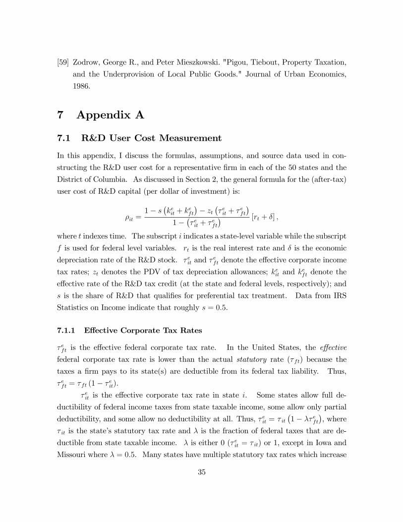
[59] Zodrow, George R., and Peter Mieszkowski. "Pigou, Tiebout, Property Taxation,
and the Underprovision of Local Public Goods." Journal of Urban Economics,
1986.
7 Appendix A
7.1 R&D User Cost Measurement
In this appendix, I discuss the formulas, assumptions, and source data used in con-
structing the R&D user cost for a representative �rm in each of the 50 states and the
District of Columbia. As discussed in Section 2, the general formula for the (after-tax)
user cost of R&D capital (per dollar of investment) is:
�it =1� s
�keit + k
eft
�� zt
�� eit + �
eft
�1�
�� eit + �
eft
� [rt + �] ;
where t indexes time. The subscript i indicates a state-level variable while the subscript
f is used for federal level variables. rt is the real interest rate and � is the economic
depreciation rate of the R&D stock. � eit and �eft denote the e¤ective corporate income
tax rates; zt denotes the PDV of tax depreciation allowances; keit and keft denote the
e¤ective rate of the R&D tax credit (at the state and federal levels, respectively); and
s is the share of R&D that quali�es for preferential tax treatment. Data from IRS
Statistics on Income indicate that roughly s = 0:5.
7.1.1 E¤ective Corporate Tax Rates
� eft is the e¤ective federal corporate tax rate. In the United States, the e¤ective
federal corporate tax rate is lower than the actual statutory rate (� ft) because the
taxes a �rm pays to its state(s) are deductible from its federal tax liability. Thus,
� eft = � ft (1� � eit).� eit is the e¤ective corporate tax rate in state i. Some states allow full de-
ductibility of federal income taxes from state taxable income, some allow only partial
deductibility, and some allow no deductibility at all. Thus, � eit = � it�1� �� eft
�, where
� it is the state�s statutory tax rate and � is the fraction of federal taxes that are de-
ductible from state taxable income. � is either 0 (� eit = � it) or 1, except in Iowa and
Missouri where � = 0:5. Many states have multiple statutory tax rates which increase
35
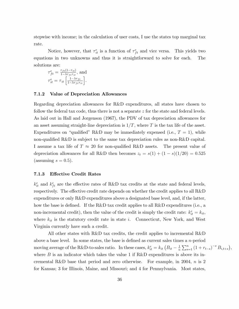
stepwise with income; in the calculation of user costs, I use the states top marginal tax
rate.
Notice, however, that � eit is a function of �eft and vice versa. This yields two
equations in two unknowns and thus it is straightforward to solve for each. The
solutions are:
� eft =�ft(1�� it)1���ft� it ; and
� eit = � it
h1���ft1���ft� it
i.
7.1.2 Value of Depreciation Allowances
Regarding depreciation allowances for R&D expenditures, all states have chosen to
follow the federal tax code, thus there is not a separate z for the state and federal levels.
As laid out in Hall and Jorgenson (1967), the PDV of tax depreciation allowances for
an asset assuming straight-line depreciation is 1=T , where T is the tax life of the asset.
Expenditures on �quali�ed�R&D may be immediately expensed (i.e., T = 1), while
non-quali�ed R&D is subject to the same tax depreciation rules as non-R&D capital.
I assume a tax life of T � 20 for non-quali�ed R&D assets. The present value of
depreciation allowances for all R&D then becomes zt = s(1) + (1 � s)(1=20) = 0:525(assuming s = 0:5).
7.1.3 E¤ective Credit Rates
keit and keft are the e¤ective rates of R&D tax credits at the state and federal levels,
respectively. The e¤ective credit rate depends on whether the credit applies to all R&D
expenditures or only R&D expenditures above a designated base level, and, if the latter,
how the base is de�ned. If the R&D tax credit applies to all R&D expenditures (i.e., a
non-incremental credit), then the value of the credit is simply the credit rate: keit = kit,
where kit is the statutory credit rate in state i. Connecticut, New York, and West
Virginia currently have such a credit.
All other states with R&D tax credits, the credit applies to incremental R&D
above a base level. In some states, the base is de�ned as current sales times a n-period
moving average of the R&D-to-sales ratio. In these cases, keit = kit�Bit � 1
n
Pns=1 (1 + rt�s)
�sBi;t+s�,
where B is an indicator which takes the value 1 if R&D expenditures is above its in-
cremental R&D base that period and zero otherwise. For example, in 2004, n is 2
for Kansas; 3 for Illinois, Maine, and Missouri; and 4 for Pennsylvania. Most states,
36
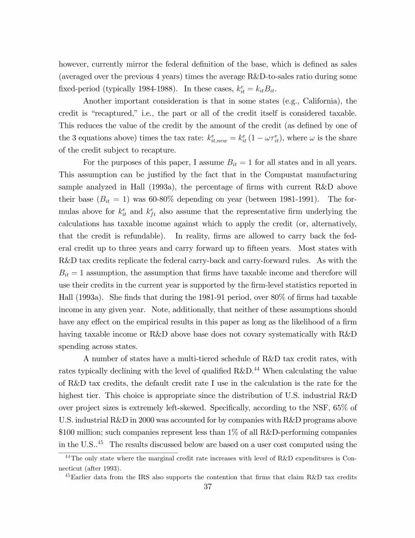
however, currently mirror the federal de�nition of the base, which is de�ned as sales
(averaged over the previous 4 years) times the average R&D-to-sales ratio during some
�xed-period (typically 1984-1988). In these cases, keit = kitBit.
Another important consideration is that in some states (e.g., California), the
credit is �recaptured,� i.e., the part or all of the credit itself is considered taxable.
This reduces the value of the credit by the amount of the credit (as de�ned by one of
the 3 equations above) times the tax rate: keit;new = keit (1� !� eit), where ! is the share
of the credit subject to recapture.
For the purposes of this paper, I assume Bit = 1 for all states and in all years.
This assumption can be justi�ed by the fact that in the Compustat manufacturing
sample analyzed in Hall (1993a), the percentage of �rms with current R&D above
their base (Bit = 1) was 60-80% depending on year (between 1981-1991). The for-
mulas above for keit and keft also assume that the representative �rm underlying the
calculations has taxable income against which to apply the credit (or, alternatively,
that the credit is refundable). In reality, �rms are allowed to carry back the fed-
eral credit up to three years and carry forward up to �fteen years. Most states with
R&D tax credits replicate the federal carry-back and carry-forward rules. As with the
Bit = 1 assumption, the assumption that �rms have taxable income and therefore will
use their credits in the current year is supported by the �rm-level statistics reported in
Hall (1993a). She �nds that during the 1981-91 period, over 80% of �rms had taxable
income in any given year. Note, additionally, that neither of these assumptions should
have any e¤ect on the empirical results in this paper as long as the likelihood of a �rm
having taxable income or R&D above base does not covary systematically with R&D
spending across states.
A number of states have a multi-tiered schedule of R&D tax credit rates, with
rates typically declining with the level of quali�ed R&D.44 When calculating the value
of R&D tax credits, the default credit rate I use in the calculation is the rate for the
highest tier. This choice is appropriate since the distribution of U.S. industrial R&D
over project sizes is extremely left-skewed. Speci�cally, according to the NSF, 65% of
U.S. industrial R&D in 2000 was accounted for by companies with R&D programs above
$100 million; such companies represent less than 1% of all R&D-performing companies
in the U.S..45 The results discussed below are based on a user cost computed using the44The only state where the marginal credit rate increases with level of R&D expenditures is Con-
necticut (after 1993).45Earlier data from the IRS also supports the contention that �rms that claim R&D tax credits
37
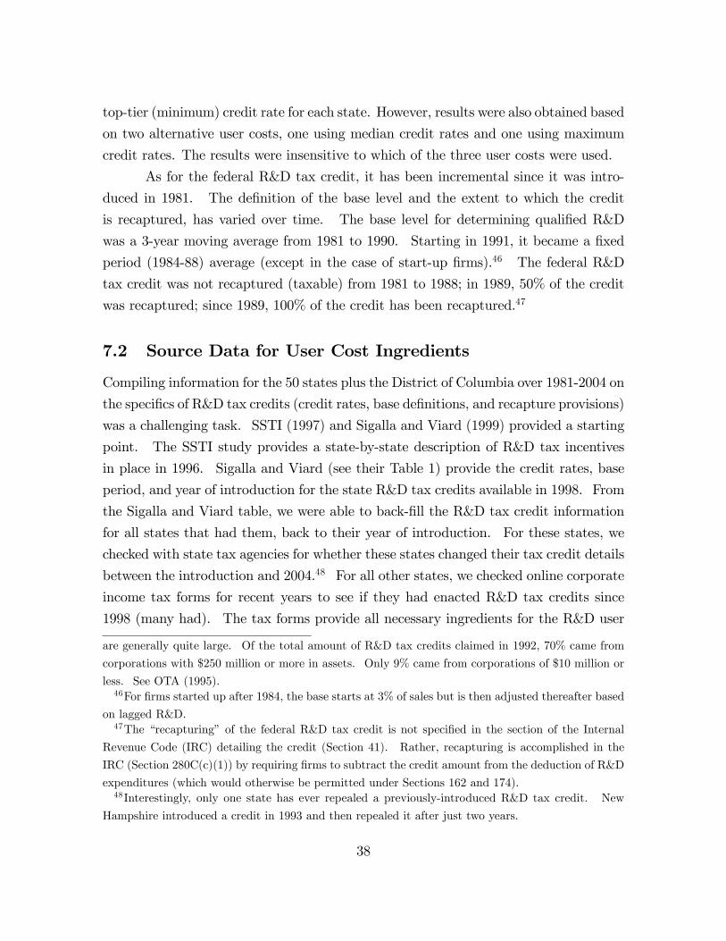
top-tier (minimum) credit rate for each state. However, results were also obtained based
on two alternative user costs, one using median credit rates and one using maximum
credit rates. The results were insensitive to which of the three user costs were used.
As for the federal R&D tax credit, it has been incremental since it was intro-
duced in 1981. The de�nition of the base level and the extent to which the credit
is recaptured, has varied over time. The base level for determining quali�ed R&D
was a 3-year moving average from 1981 to 1990. Starting in 1991, it became a �xed
period (1984-88) average (except in the case of start-up �rms).46 The federal R&D
tax credit was not recaptured (taxable) from 1981 to 1988; in 1989, 50% of the credit
was recaptured; since 1989, 100% of the credit has been recaptured.47
7.2 Source Data for User Cost Ingredients
Compiling information for the 50 states plus the District of Columbia over 1981-2004 on
the speci�cs of R&D tax credits (credit rates, base de�nitions, and recapture provisions)
was a challenging task. SSTI (1997) and Sigalla and Viard (1999) provided a starting
point. The SSTI study provides a state-by-state description of R&D tax incentives
in place in 1996. Sigalla and Viard (see their Table 1) provide the credit rates, base
period, and year of introduction for the state R&D tax credits available in 1998. From
the Sigalla and Viard table, we were able to back-�ll the R&D tax credit information
for all states that had them, back to their year of introduction. For these states, we
checked with state tax agencies for whether these states changed their tax credit details
between the introduction and 2004.48 For all other states, we checked online corporate
income tax forms for recent years to see if they had enacted R&D tax credits since
1998 (many had). The tax forms provide all necessary ingredients for the R&D user
are generally quite large. Of the total amount of R&D tax credits claimed in 1992, 70% came from
corporations with $250 million or more in assets. Only 9% came from corporations of $10 million or
less. See OTA (1995).46For �rms started up after 1984, the base starts at 3% of sales but is then adjusted thereafter based
on lagged R&D.47The �recapturing� of the federal R&D tax credit is not speci�ed in the section of the Internal
Revenue Code (IRC) detailing the credit (Section 41). Rather, recapturing is accomplished in the
IRC (Section 280C(c)(1)) by requiring �rms to subtract the credit amount from the deduction of R&D
expenditures (which would otherwise be permitted under Sections 162 and 174).48Interestingly, only one state has ever repealed a previously-introduced R&D tax credit. New
Hampshire introduced a credit in 1993 and then repealed it after just two years.
38
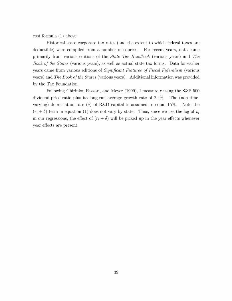
cost formula (1) above.
Historical state corporate tax rates (and the extent to which federal taxes are
deductible) were compiled from a number of sources. For recent years, data came
primarily from various editions of the State Tax Handbook (various years) and The
Book of the States (various years), as well as actual state tax forms. Data for earlier
years came from various editions of Signi�cant Features of Fiscal Federalism (various
years) andThe Book of the States (various years). Additional information was provided
by the Tax Foundation.
Following Chirinko, Fazzari, and Meyer (1999), I measure r using the S&P 500
dividend-price ratio plus its long-run average growth rate of 2.4%. The (non-time-
varying) depreciation rate (�) of R&D capital is assumed to equal 15%. Note the
(rt + �) term in equation (1) does not vary by state. Thus, since we use the log of �tin our regressions, the e¤ect of (rt + �) will be picked up in the year e¤ects whenever
year e¤ects are present.
39
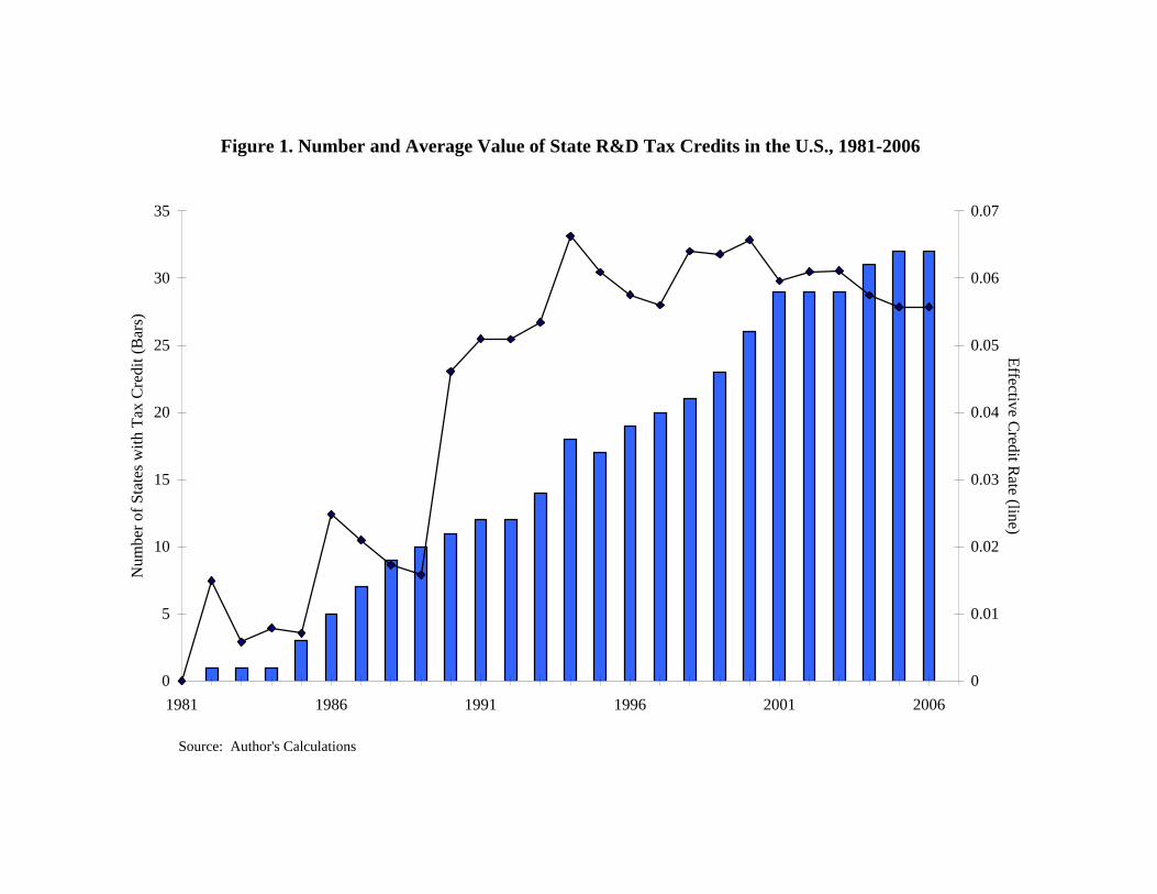
Figure 1. Number and Average Value of State R&D Tax Credits in the U.S., 1981-2006
0
5
10
15
20
25
30
35
1981 1986 1991 1996 2001 2006
Num
ber o
f Sta
tes w
ith T
ax C
redi
t (B
ars)
0
0.01
0.02
0.03
0.04
0.05
0.06
0.07
Effective Credit R
ate (line)
Source: Author's Calculations
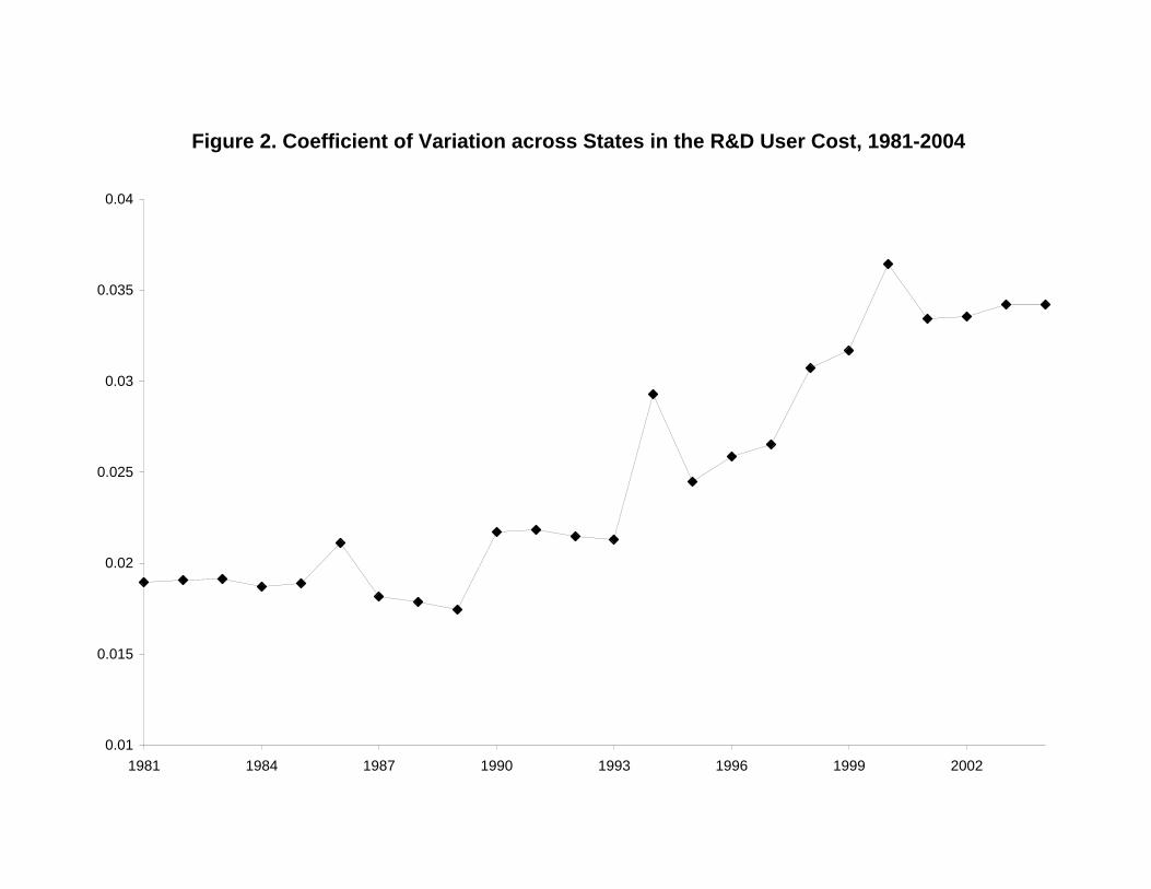
Figure 2. Coefficient of Variation across States in the R&D User Cost, 1981-2004
0.01
0.015
0.02
0.025
0.03
0.035
0.04
1981 1984 1987 1990 1993 1996 1999 2002
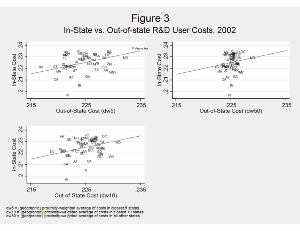
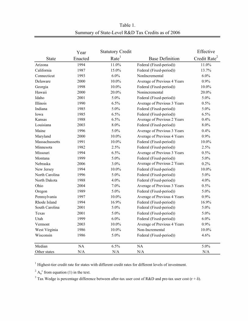
StateYear
EnactedStatutory Credit
Rate1 Base DefinitionEffective
Credit Rate2
Arizona 1994 11.0% Federal (Fixed-period)) 11.0%California 1987 15.0% Federal (Fixed-period)) 13.7%Connecticut 1993 6.0% NonIncremental 6.0%Delaware 2000 10.0% Average of Previous 4 Years 0.9%Georgia 1998 10.0% Federal (Fixed-period)) 10.0%Hawaii 2000 20.0% Nonincremental 20.0%Idaho 2001 5.0% Federal (Fixed-period)) 5.0%Illinois 1990 6.5% Average of Previous 3 Years 0.5%Indiana 1985 5.0% Federal (Fixed-period)) 5.0%Iowa 1985 6.5% Federal (Fixed-period)) 6.5%Kansas 1988 6.5% Average of Previous 2 Years 0.4%Louisiana 2003 8.0% Federal (Fixed-period)) 8.0%Maine 1996 5.0% Average of Previous 3 Years 0.4%Maryland 2000 10.0% Average of Previous 4 Years 0.9%Massachussetts 1991 10.0% Federal (Fixed-period)) 10.0%Minnesota 1982 2.5% Federal (Fixed-period)) 2.5%Missouri 1994 6.5% Average of Previous 3 Years 0.5%Montana 1999 5.0% Federal (Fixed-period)) 5.0%Nebraska 2006 3.0% Average of Previous 2 Years 0.2%New Jersey 1994 10.0% Federal (Fixed-period)) 10.0%North Carolina 1996 5.0% Federal (Fixed-period)) 5.0%North Dakota 1988 4.0% Federal (Fixed-period)) 4.0%Ohio 2004 7.0% Average of Previous 3 Years 0.5%Oregon 1989 5.0% Federal (Fixed-period)) 5.0%Pennsylvania 1997 10.0% Average of Previous 4 Years 0.9%Rhode Island 1994 16.9% Federal (Fixed-period)) 16.9%South Carolina 2001 5.0% Federal (Fixed-period)) 5.0%Texas 2001 5.0% Federal (Fixed-period)) 5.0%Utah 1999 6.0% Federal (Fixed-period)) 6.0%Vermont 2003 10.0% Average of Previous 4 Years 0.9%West Virginia 1986 10.0% Non-Incremental 10.0%Wisconsin 1986 5.0% Federal (Fixed-period)) 4.6%
Median NA 6.5% NA 5.0%Other states N/A N/A N/A N/A
Table 1.
3 Tax Wedge is percentage difference between after-tax user cost of R&D and pre-tax user cost (r + δ).
Summary of State-Level R&D Tax Credits as of 2006
2 Aitc from equation (1) in the text.
1 Highest-tier credit rate for states with different credit rates for different levels of investment.
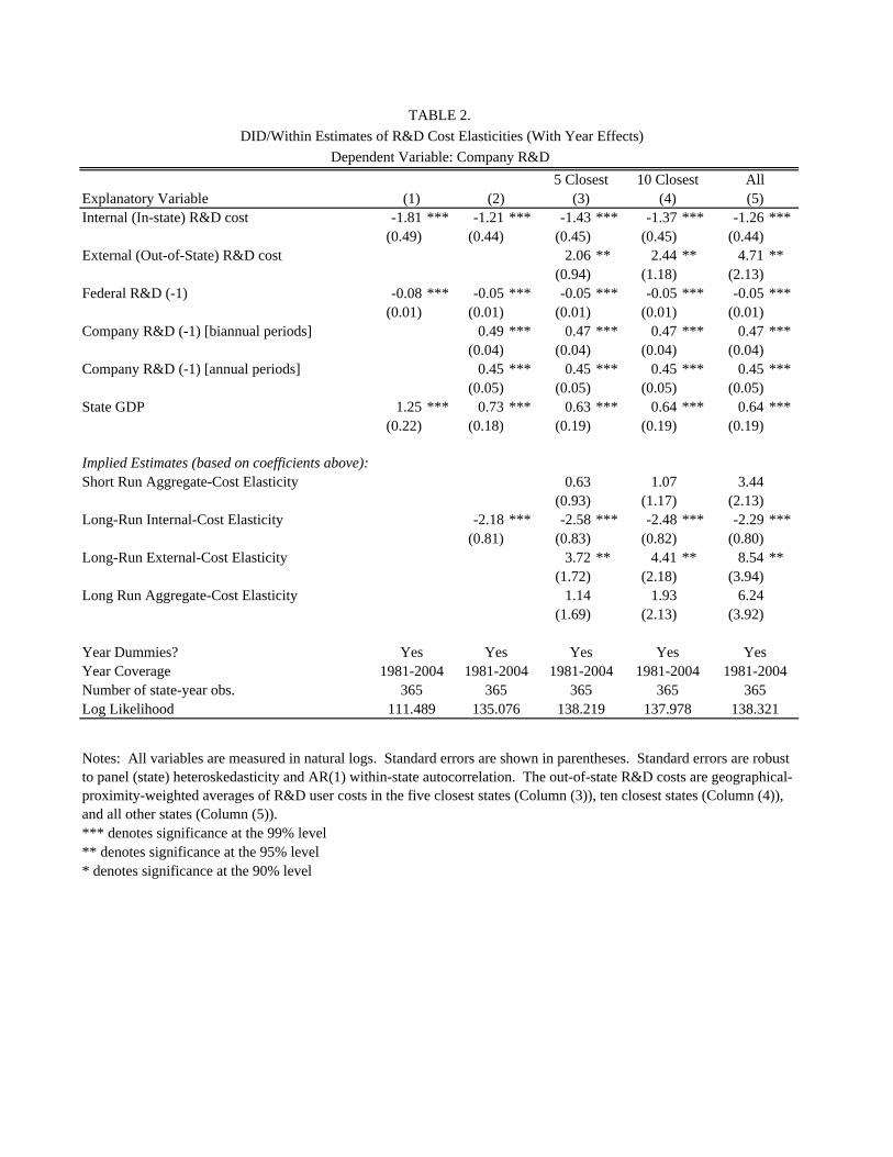
DID/Within Estimates of R&D Cost Elasticities (With Year Effects)Dependent Variable: Company R&D
Explanatory VariableInternal (In-state) R&D cost -1.81 *** -1.21 *** -1.43 *** -1.37 *** -1.26 ***
(0.49) (0.44) (0.45) (0.45) (0.44)External (Out-of-State) R&D cost 2.06 ** 2.44 ** 4.71 **
(0.94) (1.18) (2.13)Federal R&D (-1) -0.08 *** -0.05 *** -0.05 *** -0.05 *** -0.05 ***
(0.01) (0.01) (0.01) (0.01) (0.01)Company R&D (-1) [biannual periods] 0.49 *** 0.47 *** 0.47 *** 0.47 ***
(0.04) (0.04) (0.04) (0.04)Company R&D (-1) [annual periods] 0.45 *** 0.45 *** 0.45 *** 0.45 ***
(0.05) (0.05) (0.05) (0.05)State GDP 1.25 *** 0.73 *** 0.63 *** 0.64 *** 0.64 ***
(0.22) (0.18) (0.19) (0.19) (0.19)
Implied Estimates (based on coefficients above):Short Run Aggregate-Cost Elasticity 0.63 1.07 3.44
(0.93) (1.17) (2.13)Long-Run Internal-Cost Elasticity -2.18 *** -2.58 *** -2.48 *** -2.29 ***
(0.81) (0.83) (0.82) (0.80)Long-Run External-Cost Elasticity 3.72 ** 4.41 ** 8.54 **
(1.72) (2.18) (3.94)Long Run Aggregate-Cost Elasticity 1.14 1.93 6.24
(1.69) (2.13) (3.92)
Year Dummies?Year CoverageNumber of state-year obs.Log Likelihood
*** denotes significance at the 99% level** denotes significance at the 95% level* denotes significance at the 90% level
Notes: All variables are measured in natural logs. Standard errors are shown in parentheses. Standard errors are robust to panel (state) heteroskedasticity and AR(1) within-state autocorrelation. The out-of-state R&D costs are geographical-proximity-weighted averages of R&D user costs in the five closest states (Column (3)), ten closest states (Column (4)), and all other states (Column (5)).
YesYes1981-2004
Yes
365137.978
365138.219
TABLE 2.
5 Closest All10 Closest(1)
111.489
Yes1981-20041981-2004
365
(2)
365135.076
(3) (4) (5)
1981-2004365
138.321
Yes1981-2004
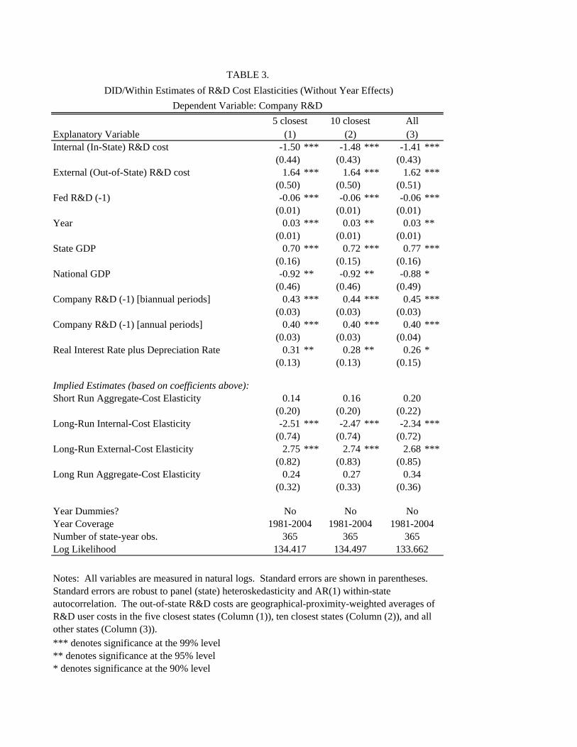
DID/Within Estimates of R&D Cost Elasticities (Without Year Effects)Dependent Variable: Company R&D
Explanatory VariableInternal (In-State) R&D cost -1.50 *** -1.48 *** -1.41 ***
(0.44) (0.43) (0.43)External (Out-of-State) R&D cost 1.64 *** 1.64 *** 1.62 ***
(0.50) (0.50) (0.51)Fed R&D (-1) -0.06 *** -0.06 *** -0.06 ***
(0.01) (0.01) (0.01)Year 0.03 *** 0.03 ** 0.03 **
(0.01) (0.01) (0.01)State GDP 0.70 *** 0.72 *** 0.77 ***
(0.16) (0.15) (0.16)National GDP -0.92 ** -0.92 ** -0.88 *
(0.46) (0.46) (0.49)Company R&D (-1) [biannual periods] 0.43 *** 0.44 *** 0.45 ***
(0.03) (0.03) (0.03)Company R&D (-1) [annual periods] 0.40 *** 0.40 *** 0.40 ***
(0.03) (0.03) (0.04)Real Interest Rate plus Depreciation Rate 0.31 ** 0.28 ** 0.26 *
(0.13) (0.13) (0.15)
Implied Estimates (based on coefficients above):Short Run Aggregate-Cost Elasticity 0.14 0.16 0.20
(0.20) (0.20) (0.22)Long-Run Internal-Cost Elasticity -2.51 *** -2.47 *** -2.34 ***
(0.74) (0.74) (0.72)Long-Run External-Cost Elasticity 2.75 *** 2.74 *** 2.68 ***
(0.82) (0.83) (0.85)Long Run Aggregate-Cost Elasticity 0.24 0.27 0.34
(0.32) (0.33) (0.36)
Year Dummies?Year CoverageNumber of state-year obs.Log Likelihood
*** denotes significance at the 99% level** denotes significance at the 95% level* denotes significance at the 90% level
No No
TABLE 3.
(1) (2) (3)5 closest 10 closest All
No
365 365 3651981-2004 1981-2004 1981-2004
Notes: All variables are measured in natural logs. Standard errors are shown in parentheses. Standard errors are robust to panel (state) heteroskedasticity and AR(1) within-state autocorrelation. The out-of-state R&D costs are geographical-proximity-weighted averages of R&D user costs in the five closest states (Column (1)), ten closest states (Column (2)), and all other states (Column (3)).
134.417 134.497 133.662
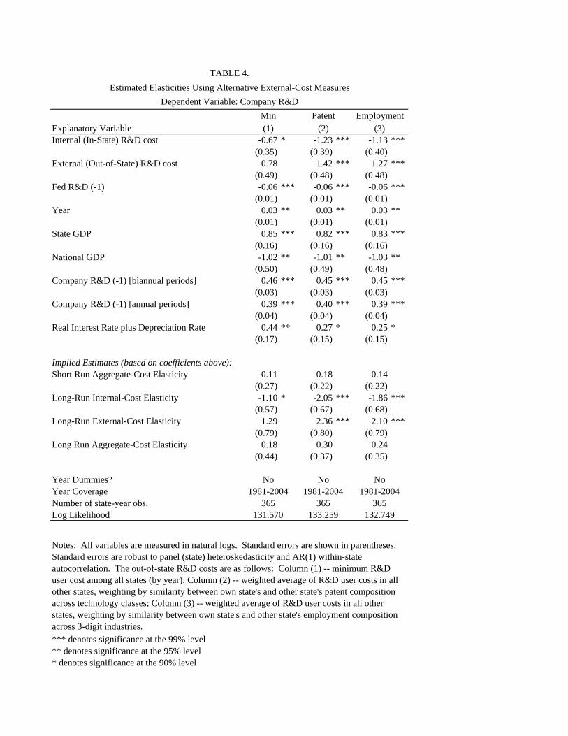
Estimated Elasticities Using Alternative External-Cost MeasuresDependent Variable: Company R&D
Explanatory VariableInternal (In-State) R&D cost -0.67 * -1.23 *** -1.13 ***
(0.35) (0.39) (0.40)External (Out-of-State) R&D cost 0.78 1.42 *** 1.27 ***
(0.49) (0.48) (0.48)Fed R&D (-1) -0.06 *** -0.06 *** -0.06 ***
(0.01) (0.01) (0.01)Year 0.03 ** 0.03 ** 0.03 **
(0.01) (0.01) (0.01)State GDP 0.85 *** 0.82 *** 0.83 ***
(0.16) (0.16) (0.16)National GDP -1.02 ** -1.01 ** -1.03 **
(0.50) (0.49) (0.48)Company R&D (-1) [biannual periods] 0.46 *** 0.45 *** 0.45 ***
(0.03) (0.03) (0.03)Company R&D (-1) [annual periods] 0.39 *** 0.40 *** 0.39 ***
(0.04) (0.04) (0.04)Real Interest Rate plus Depreciation Rate 0.44 ** 0.27 * 0.25 *
(0.17) (0.15) (0.15)
Implied Estimates (based on coefficients above):Short Run Aggregate-Cost Elasticity 0.11 0.18 0.14
(0.27) (0.22) (0.22)Long-Run Internal-Cost Elasticity -1.10 * -2.05 *** -1.86 ***
(0.57) (0.67) (0.68)Long-Run External-Cost Elasticity 1.29 2.36 *** 2.10 ***
(0.79) (0.80) (0.79)Long Run Aggregate-Cost Elasticity 0.18 0.30 0.24
(0.44) (0.37) (0.35)
Year Dummies?Year CoverageNumber of state-year obs.Log Likelihood
*** denotes significance at the 99% level** denotes significance at the 95% level* denotes significance at the 90% level
TABLE 4.
Min Patent Employment(1) (2) (3)
No No No1981-2004 1981-2004 1981-2004
365 365 365
Notes: All variables are measured in natural logs. Standard errors are shown in parentheses. Standard errors are robust to panel (state) heteroskedasticity and AR(1) within-state autocorrelation. The out-of-state R&D costs are as follows: Column (1) -- minimum R&D user cost among all states (by year); Column (2) -- weighted average of R&D user costs in all other states, weighting by similarity between own state's and other state's patent composition across technology classes; Column (3) -- weighted average of R&D user costs in all other states, weighting by similarity between own state's and other state's employment composition across 3-digit industries.
131.570 133.259 132.749
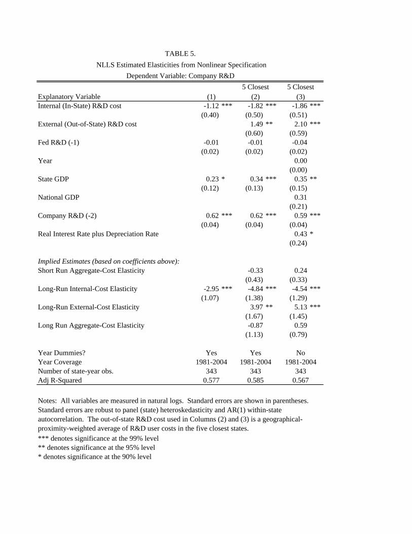
NLLS Estimated Elasticities from Nonlinear SpecificationDependent Variable: Company R&D
Explanatory VariableInternal (In-State) R&D cost -1.12 *** -1.82 *** -1.86 ***
(0.40) (0.50) (0.51)External (Out-of-State) R&D cost 1.49 ** 2.10 ***
(0.60) (0.59)Fed R&D (-1) -0.01 -0.01 -0.04
(0.02) (0.02) (0.02)Year 0.00
(0.00)State GDP 0.23 * 0.34 *** 0.35 **
(0.12) (0.13) (0.15)National GDP 0.31
(0.21)Company R&D (-2) 0.62 *** 0.62 *** 0.59 ***
(0.04) (0.04) (0.04)Real Interest Rate plus Depreciation Rate 0.43 *
(0.24)
Implied Estimates (based on coefficients above):Short Run Aggregate-Cost Elasticity -0.33 0.24
(0.43) (0.33)Long-Run Internal-Cost Elasticity -2.95 *** -4.84 *** -4.54 ***
(1.07) (1.38) (1.29)Long-Run External-Cost Elasticity 3.97 ** 5.13 ***
(1.67) (1.45)Long Run Aggregate-Cost Elasticity -0.87 0.59
(1.13) (0.79)
Year Dummies?Year CoverageNumber of state-year obs.Adj R-Squared
*** denotes significance at the 99% level** denotes significance at the 95% level* denotes significance at the 90% level
TABLE 5.
5 Closest 5 Closest
0.585 0.567
(1) (2) (3)
Yes Yes No
Notes: All variables are measured in natural logs. Standard errors are shown in parentheses. Standard errors are robust to panel (state) heteroskedasticity and AR(1) within-state autocorrelation. The out-of-state R&D cost used in Columns (2) and (3) is a geographical-proximity-weighted average of R&D user costs in the five closest states.
1981-2004 1981-2004 1981-2004343 343 343
0.577
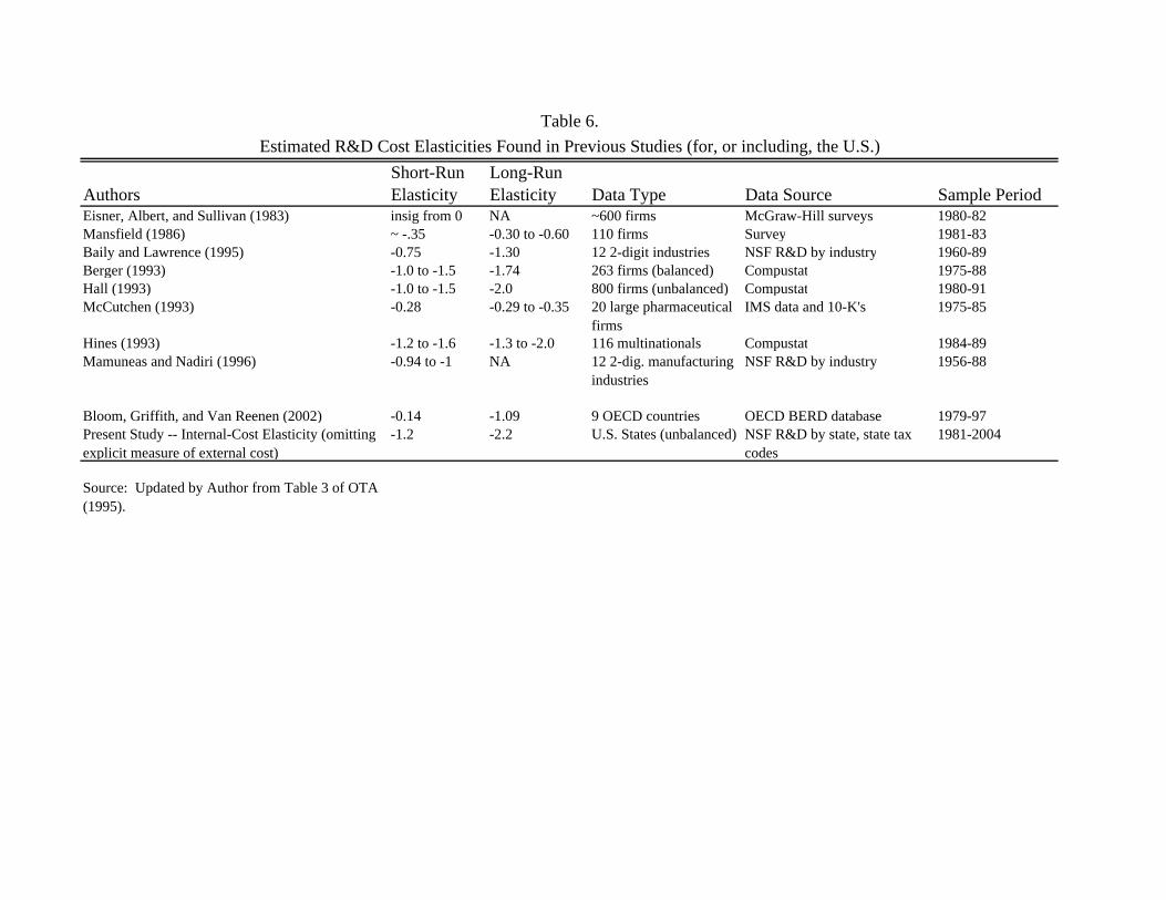
AuthorsShort-Run Elasticity
Long-Run Elasticity Data Type Data Source Sample Period
Eisner, Albert, and Sullivan (1983) insig from 0 NA ~600 firms McGraw-Hill surveys 1980-82Mansfield (1986) ~ -.35 -0.30 to -0.60 110 firms Survey 1981-83Baily and Lawrence (1995) -0.75 -1.30 12 2-digit industries NSF R&D by industry 1960-89Berger (1993) -1.0 to -1.5 -1.74 263 firms (balanced) Compustat 1975-88Hall (1993) -1.0 to -1.5 -2.0 800 firms (unbalanced) Compustat 1980-91McCutchen (1993) -0.28 -0.29 to -0.35 20 large pharmaceutical
firmsIMS data and 10-K's 1975-85
Hines (1993) -1.2 to -1.6 -1.3 to -2.0 116 multinationals Compustat 1984-89Mamuneas and Nadiri (1996) -0.94 to -1 NA 12 2-dig. manufacturing
industriesNSF R&D by industry 1956-88
Bloom, Griffith, and Van Reenen (2002) -0.14 -1.09 9 OECD countries OECD BERD database 1979-97Present Study -- Internal-Cost Elasticity (omitting explicit measure of external cost)
-1.2 -2.2 U.S. States (unbalanced) NSF R&D by state, state tax codes
1981-2004
Source: Updated by Author from Table 3 of OTA (1995).
Table 6.Estimated R&D Cost Elasticities Found in Previous Studies (for, or including, the U.S.)
Top Related