


Languages
Pages
Legal

Bayes Factors 1
Running head: BAYES FACTORS
Bayes Factor Approaches for Testing Interval Null Hypotheses
Richard D. Morey
University of Groningen
Jeffrey N. Rouder
University of Missouri
Richard D. Morey
DMPG
Grote Kruisstraat 2/1
9712NS Groningen
The Netherlands
Bayes Factors 2
Abstract
Psychological theories are statements of constraint. The role of hypothesis testing in
psychology is to test whether specific theoretical constraints hold in data. Bayesian
statistics is well-suited the task of finding supporting evidence for constraint, because it
allows for comparing evidence for two hypotheses against one another. One issue in
hypothesis testing is that constraints may hold only approximately rather than exactly,
and the reason for small deviations may be trivial or uninteresting. In the large-sample
limit, these uninteresting, small deviations will lead to the rejection of a useful constraint.
In this paper, we develop several Bayes factor one-sample tests for the assessment of
approximate equality and ordinal constraints. In these tests, the null hypothesis covers a
small interval of nonzero but negligible effect sizes around zero. These Bayes factors are
alternatives to previously-developed Bayes factors, which do not allow for interval null
hypotheses, and may especially prove useful to researchers who use statistical equivalence
testing. To facilitate adoption of these Bayes factor tests, we provide easy-to-use software.

Bayes Factors 3
Bayes Factor Approaches for Testing Interval Null Hypotheses
The usefulness of psychological theories is determined by the extent to which they
make constrained predictions about data. In many cases, these constraints are ordinal in
nature: participants are predicted to perform better in one condition than another, or
participants with a certain characteristic are predicted to perform better than those
without this characteristic. In some cases, the predictions are stronger; they are about
equalities. One example is the Fechner-Weber law, which describes the amount of
intensity, ∆I, that must be added to a background of intensity I for successful
discrimination. The law states that performance varies as ∆I/I; the constraint is that
when the intensity of an increment and background are both multiplied by the same
constant, detection performance will be the same. Another example of a theoretically
interesting equality constraint is the lack of effect of gender on certain tasks (Shibley
Hyde, 2005, 2007) or a lack of interaction across specified manipulations (e.g., additive
factors, Sternberg, 1969). Furthermore, the assessment of formal models – for example,
structural equation models – is a matter of assessing equality constraints. The assessment
of both equality and ordinal constraints is the primary use of hypothesis testing in the
psychological sciences. In this paper, we develop Bayes factor methods for evaluating
evidence for constraints in data. In the following development, we first focus on assessing
evidence for equality constraints, and then generalize the approach to ordinal constraints.
Our development of Bayes factor tests for equality constraints is motivated by
several common critiques of null-hypothesis significance tests (NHST). One critique of
testing for equality constraints is that such constraints are not plausible; that is, small
violations of equality constraints always exist (Cohen, 1994; Meehl, 1987). A second
critique is that null hypothesis significance tests are asymmetric in that equality
constraints may only be rejected and not accepted. These two critiques provide rationales

Bayes Factors 4
for statistical equivalence tests, in which approximate equality constraints serve as the
alternative hypothesis rather than the default, null hypothesis. The third critique is that
the asymmetry in choosing default hypotheses, whether the null or alternative, leads to
inference that overstates the evidence against the default hypothesis (Berger & Sellke,
1987; Rouder et al., 2009; Sellke, Bayarri, & Berger, 2001; Wagenmakers, 2007). This
third critique serves as motivation for the use of Bayes factors. In this paper we develop
Bayes factor tests that allow for equivalence regions.
Nil Hypotheses, Null Hypotheses, and Equivalence Regions
Equality constraints may be represented as point-null hypotheses. Without any loss
of generality, any point hypothesis can be expressed as a nil hypothesis; that is, the
statement that a parameter of interest is zero (Cohen, 1994)1. Nil hypotheses are
statements such as: one variable has no effect on an another; there is no difference
between two variables; there is no association between two variables; or, the parameter
has a specific value. In order to mitigate confusion, we will use the following terminology
throughout: the nil hypothesis refers to the point hypothesis that the parameter is
identically 0. The null hypothesis is more general: it may be restricted to a nil hypothesis
or may allow for values which deviate slightly from the nil. The null hypothesis therefore
may capture nonzero effects that are too small to be of interest. A third type of
hypothesis, the default hypothesis, refers to a hypothesis assumed true unless sufficient
evidence is found against it. The nil hypothesis is the default hypothesis in most null
hypothesis significance tests, but not in statistical equivalence testing.
Cohen (1994), among others (Berger & Delampady, 1987; Berkson, 1938; Meehl,
1978), offers the viewpoint that nil hypotheses never hold to an arbitrary level of
precision; that is, a priori nil hypotheses are false. For instance, the Fechner-Weber law,
discussed above cannot hold to arbitrary precision because at some level, the process

Bayes Factors 5
becomes discretized (if for no other reason than light itself is quantal in nature). As
another example, a researcher might be interested in whether a particular genetic
mutation correlates with educational outcomes. Even if the gene codes for something
unrelated – say, hair growth rate – it seems unlikely that in the population, people with
the mutation have exactly the same educational outcomes as those without. The main
point in these examples is that the nil will fail for trivial or uninteresting reasons. Meehl
(1978) refers to the trivial relationships that variables have to others as the “crud factor”
in psychological research.
In this paper, we take as a default position that the nil never holds to arbitrary
precision. The fact that nil hypotheses may break down, however, is not an argument
against their usefulness in many areas of psychological research. Often these nil
hypotheses are good approximations and are exceedingly useful for guiding theory
development. For instance, even though the Fechner-Weber Law breaks down for very low
intensities, it may nonetheless provide appropriate constraint on the mechanisms of
perceptual decision making. Likewise, even though the equality of men and women in the
performance of a certain task may break down in some limit, it is still useful in suggesting
that the mental processing underlying the task may not vary across gender. Hence, the
argument that the nil hypothesis is never exactly correct is not an argument against
proposing constraints. The fact that the nil hypothesis is never true is, however, an
important consideration when performing statistical tests. A key goal in our development
are methods that do not reject null hypotheses if the failure is due to trivially small effects.
One solution is to abandon point hypotheses altogether. Hodges and Lehmann
(1954) suggested establishing a region of parameter values around the nil hypothesis that
are not “materially significant” – that is, although the true parameter value may indeed
be slightly different from the nil hypothesis value, the nil hypothesis would still be
preferred for parsimony’s sake. This same logic is adopted by the statistical equivalence

Bayes Factors 6
test (SET) paradigm (Rogers, Howard, & Vessey, 1993; Wellek, 2003). In SET, an
“equivalence” region is defined on a parameter of interest. This equivalence region
contains all parameter values which may be considered too small to be meaningfully
different from 0. The researcher specifies this equivalence region before analysis and its
size is informed by substantive considerations in the domain at hand.
One way to formulate a statistical equivalence test is with confidence intervals, as
shown in Figure 1. The equivalence region in the figure is defined from -0.2 to 0.2. All
parameter values within these bounds are considered “equivalent” to 0. The default
hypothesis is nonequivalence: that is, the parameter is outside the equivalence region.
Because the nonequivalence hypotheses is default, we reject nonequivalence only with
sufficient evidence and retain nonequivalence otherwise. Evidence in this formulation is
the relationship of confidence intervals to the equivalence bounds. If the 100(1− 2α)%
confidence interval lies within the equivalence region, then nonequivalence is rejected.
Shown in the figure are hypothetical CIs for four samples. The confidence intervals for
Samples A, B, and D do not provide sufficient evidence to reject nonequivalence. The
confidence interval for Sample C, however, only contains values in the equivalence region.
For Sample C, the nonequivalence null hypothesis may be rejected in favor of equivalence.
Relative Evidence
The methods discussed above are all based on the idea of controlling the rates of
certain kinds of errors. This is the traditional NHST approach; Type I error rate is held at
a rate of α, or CIs are built which fail to cover the true value at a rate of α. However, it is
often useful in scientific discourse to have methods which measure the evidence for
positions rather than make a binary choice between them. In both Bayesian and freqentist
statistics, the likelihood ratio is used as a measure of relative evidence between two
hypotheses (Royall, 1997). Measuring relative evidence is fairly straightforward if both

Bayes Factors 7
hypotheses are points. For instance, suppose wish to compare the evidence for the
hypothesis that µ = µa versus the hypothesis that µ = µb in a one-sample design. The two
hypotheses may be written as two models:
Ha : yiiid∼ Normal(µa,σ
2),
Hb yiiid∼ Normal(µb,σ
2),
where µa, µb, and σ2 are prespecified values. The likelihood ratio quantifying the evidence
for hypothesis Ha relative to hypothesis Hb, which we abbreviate Bab, is
Bab =Pr(Y | Ha)
Pr(Y | Hb), (1)
where Y = (y1, y2, . . . , yN ) is a vector of observations. Because the data are assumed to
be normally distributed and conditionally independent, we use the product of normal
distribution functions2 φ(y | µ,σ2) to form the likelihood ratio:
Bab =
∏Ni=1 φ(yi | µa,σ2)
∏Ni=1 φ(yi | µb,σ2)
.
The notion that relative evidence is provided by the likelihood ratio is used in both
frequentist and Bayesian paradigms.
Because most hypothesis tests in psychological research are built on the premise of
controlling Type I rates, rather than on the basis of evidence, it is interesting to ask how
much relative evidence is there in rejections of hypotheses in NHST testing (Lindley, 1957,
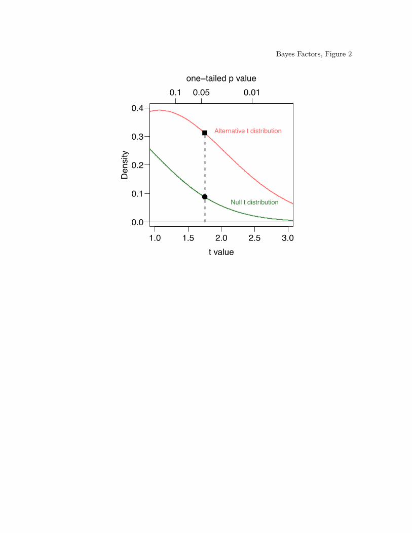
Sellke, Bayarri, & Berger, 2001). For example, consider the case of a researcher who
observes a one-sided t value of 1.75 with 30 observations. We take as Hb the nil that µ = 0
and as Ha an alternative that µ = .2σ (that is, the standardized effect size is .2), where σ,
the standard deviation, is an unknown. In this case, Pr(Y |Hb) is the density at 1.75
under the central t distribution. The Pr(Y |Ha) is the density at 1.75 under a noncentral t
with noncentrality parameter .2√30. These areas are shown in Figure 2, and the relative
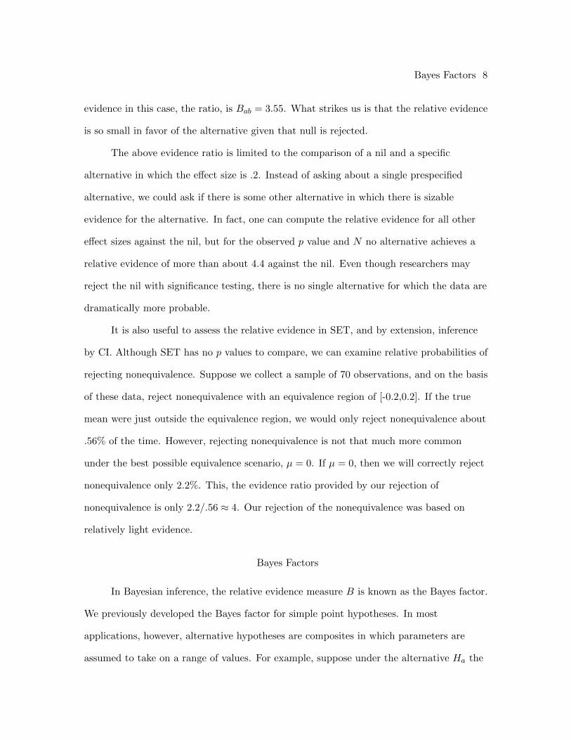
Bayes Factors 8
evidence in this case, the ratio, is Bab = 3.55. What strikes us is that the relative evidence
is so small in favor of the alternative given that null is rejected.
The above evidence ratio is limited to the comparison of a nil and a specific
alternative in which the effect size is .2. Instead of asking about a single prespecified
alternative, we could ask if there is some other alternative in which there is sizable
evidence for the alternative. In fact, one can compute the relative evidence for all other
effect sizes against the nil, but for the observed p value and N no alternative achieves a
relative evidence of more than about 4.4 against the nil. Even though researchers may
reject the nil with significance testing, there is no single alternative for which the data are
dramatically more probable.
It is also useful to assess the relative evidence in SET, and by extension, inference
by CI. Although SET has no p values to compare, we can examine relative probabilities of
rejecting nonequivalence. Suppose we collect a sample of 70 observations, and on the basis
of these data, reject nonequivalence with an equivalence region of [-0.2,0.2]. If the true
mean were just outside the equivalence region, we would only reject nonequivalence about
.56% of the time. However, rejecting nonequivalence is not that much more common
under the best possible equivalence scenario, µ = 0. If µ = 0, then we will correctly reject
nonequivalence only 2.2%. This, the evidence ratio provided by our rejection of
nonequivalence is only 2.2/.56 ≈ 4. Our rejection of the nonequivalence was based on
relatively light evidence.
Bayes Factors
In Bayesian inference, the relative evidence measure B is known as the Bayes factor.
We previously developed the Bayes factor for simple point hypotheses. In most
applications, however, alternative hypotheses are composites in which parameters are
assumed to take on a range of values. For example, suppose under the alternative Ha the

Bayes Factors 9
value of µ is allowed to range across all real numbers. In Bayesian statistics, probability is
interpreted as uncertainty; to compute the probability of data under a hypothesis, we
average over the uncertainty in the parameters. The probability of data under the
hypothesis is thus:
P (Y |Ha) =
∫
µP (Y|µ)f(µ)dµ. (2)
The term P (Y|µ) is the conditional probability density for the data given the parameter µ
(the likelihood), and the term f(µ) is the prior probability density for µ. A more general
formulation, for when a vector of parameters is free to vary under a hypothesis H, is
P (Y |H) =
∫
θ∈ΘP (Y |H,θ)f(θ|H)dθ, (3)
where θ is a vector of parameters, and Θ is the space across which the parameters vary.
The function f is the prior density of θ and describes the researchers belief or uncertainty
about the parameters before observing the data. In Bayesian analysis, the specification of
f is critical to defining the hypotheses, and is the point where subjective probability
enters Bayesian inference. We realize that frequentists may object to the
conceptualization of probability as capturing a degree or measure of belief. The argument
for subjective probability is made most elegantly in the psychological literature by
Edwards et al. (1963). We note here that subjective probability stands on firm axiomatic
foundations, and leads to ideal rules about updating beliefs in light of data (Cox, 1946; De
Finetti, 1992; Gelman, Carlin, Stern, & Rubin, 2004; Jaynes, 1986).
The marginal probability in Eq. (3) may be viewed as a weighted average across all
parameter values, with the weights for each parameter value is given by a prior
distribution. Priors that place greater weight on parameter values not concordant with
the data have lower marginal probability. This weighted averaging properly penalizes
flexibility in models in which a large set of parameters have some a priori weight (Myung,
2000). Flexible models may fit the data better (i.e. be preferred by the likelihood ratio)

Bayes Factors 10
than more constrained ones, but they will also include prior weight over unlikely
parameter values. Averaging over the prior ensures that flexible models are properly
penalized for their flexibility.
This averaging across all parameter values also reveals a key difference between
Bayesian methods and frequentist methods: the interpretation of probability as
uncertainty licenses averaging. Parameters are treated as random quantities which have
distributions that may be marginalized. In frequentist methods, however, this averaging is
not licensed; other approaches, such as computing maximum likelihood values, are used.
In Bayesian inference, it is also possible to compute the odds of competing two
hypotheses against one another, given the observed data; e.g., P (Ha|Y )/P (Hb|Y ). This
quantity, the posterior odds is related to the Bayes factor:
P (Ha|Y )
P (Hb|Y )= Bab ×
P (Ha)
P (Hb), (4)
where P (Ha)P (Hb)
is the prior odds and describes the relative degree of belief in the hypotheses
before the data are observed. The Bayes factor describes how beliefs are to be updated.
Jeffreys (1961) and Kass (1993) note that the Bayes factor is ideal for reporting evidence
because it describes how researchers should change their beliefs regardless of what those
initial beliefs are. Prior odds provide readers and analysts a mechanism to add context as
to how evidence is to be interpreted. We wish to emphasize, however, that the Bayes
factor may be interpreted as the relative evidence contributed by the data, without
stipulating prior odds.
Bayes factor for nil hypotheses
In constructing Bayes factors, different hypotheses may be implemented as different
choices of priors over parameters. For example, the nil hypothesis may be implemented by
specifying a point prior over the parameter of interest. More interesting are the priors
under the alternative. It is common when using Bayesian techniques for parameter

Bayes Factors 11
estimation to assume diffuse or “noninformative” priors (Gelman, Carlin, Stern, & Rubin,
2004) for these alternatives. These diffuse priors are used to minimize the influence of the
prior distribution on the posterior distribution. Noninformative priors are often improper,
meaning that they do not integrate to a finite number. A common improper,
noninformative prior for the mean of a normal distribution, for instance, is a constant
value over all real numbers. This constant prior corresponds to the assumption of absolute
ignorance; that is, that no value for the mean is a priori more likely than any other. As
long as the posterior distribution is proper, the impropriety of the prior poses no problem
for Bayesian parameter estimation.
For hypothesis testing, as opposed to estimation, the choice of a diffuse prior for the
alternative hypothesis is problematic. The reason is that the Bayes factor is the ratio of
the expectation of the likelihoods, taken over their respective priors. As the prior becomes
more and more diffuse, unlikely values dominate, making the expectation of the likelihood
approach 0. If the null hypothesis is a point, and the alternative prior is noninformative,
the point will be preferred, regardless of the data. Ironically, using “noninformative”
priors in Bayes factors leads to the predetermined result of always choosing the null
hypothesis (Lindley, 1957).
Jeffreys (1961) suggests placing priors on the standardized effect size, δ = µ/σ. In
this case, yi ∼ Normal(σδ,σ2). As Iverson et al. (2009) note, effect size has a natural scale
and proper priors for it are appropriate. The prior on the point nil is simply that the
effect size is exactly zero. One reasonable prior on the alternative might be that effect
sizes are distributed as a standard normal. This prior structure is inspired by the
knowledge that true effect sizes are typically not large, and that the analyst is agnostic to
the direction of any possible effect.
Although the standard normal is a reasoned choice, it is a thin-tailed distribution;
that is, large effect sizes, such as 5.0, are effectively excluded from consideration. A
Bayes Factors 12
less-informative prior would not effectively preclude the possibility of large effect sizes. To
accomplish this goal, we use a distribution with fatter tails: the t distribution, as a prior
on effect size. As the degrees of freedom of the t distribution decrease, the tails of the t
distribution become fatter; with only 1 degree of freedom, the tails of the t distribution
are fat enough that the distribution has no expected value or higher-order moments. The
t(1) distribution is also known as the standard Cauchy distribution. The standard
Cauchy-distributed prior on δ quantifies an assumption that excessively large true δ
parameters are much less plausible than small effect sizes, but are still possible. We
express the prior structure as follows:
H0 : δ = 0
H1 : δ ∼ Cauchy(r = 1),
where r is a scaling parameter, and represents one-half the interquartile range of the
Cauchy. A Cauchy distribution with r = 1 is a standard Cauchy distribution.
A prior is also needed for σ2. Because σ2 is a parameter in both models, a
noninformative prior on it is both practical and desirable:
p(σ2) ∝ 1
σ2,
where p(σ2) represents an improper prior density on σ2. The advantage of the 1/σ2 prior
is that it is the Jeffreys prior. Jeffreys priors have the desirable property that they impart
the same information, even if under transformations of parameter (Jeffreys, 1946).
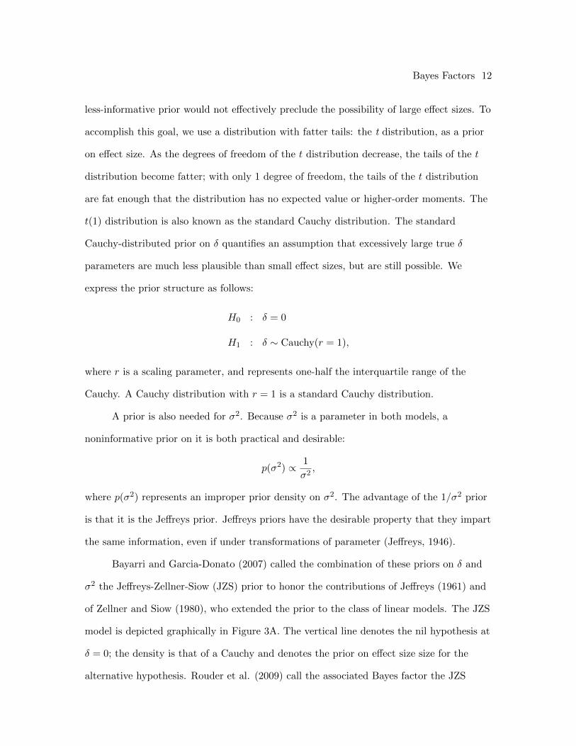
Bayarri and Garcia-Donato (2007) called the combination of these priors on δ and
σ2 the Jeffreys-Zellner-Siow (JZS) prior to honor the contributions of Jeffreys (1961) and
of Zellner and Siow (1980), who extended the prior to the class of linear models. The JZS
model is depicted graphically in Figure 3A. The vertical line denotes the nil hypothesis at
δ = 0; the density is that of a Cauchy and denotes the prior on effect size size for the
alternative hypothesis. Rouder et al. (2009) call the associated Bayes factor the JZS

Bayes Factors 13
Bayes factor. They provide expressions for the JZS Bayes factor for one- and two-sample
tests as well as a web applet for computation (http://pcl.missouri.edu/bayesfactor).
Consider the following real-world example of the differences between JZS Bayes
factor and NHST analysis. It is well-known that emotionally-evocative words are better
recognized in a memory experiment than emotionally neutral words (Murphy &
Isaacowitz, 2008). Although this increase in performance would seemingly indicate better
memory for these stimuli, this pattern may instead reflect response biases (Dougal &
Rotello, 2007; Thapar & Rouder, 2009). Thus, memory may be the same for both
emotional valence levels, but participants are simply biased to state that
emotionally-evocative words were studied more often than neutral words when guessing or
when responding with limited information. Thapar and Rouder, for example, fit a variant
of Luce’s Similarity Choice Rule (Luce, 1963) and found emotional valence effects on
response bias parameters but not in memory sensitivity parameters.
Grider and Malmberg (2008, Experiment 3) provide the following insightful test of
the equality of memory across emotional valence levels. Participants first study both
evocative and neutral words. At test, participants see a new word (the lure) as well as a
studied word (the target), and have to judge which was studied. In Grider and
Malmberg’s task, lures and targets always had the same emotional valence so that each
would be chosen equally likely in the absence of mnemonic information. With response
bias controlled, it is reasonable to conclude that an approximate equality of performance
supports the invariance of memory across emotional valence, and differences in
performance support differences in memory across emotional valence. They find mean
recognition accuracy for positive words (80%) was somewhat higher than mean
recognition accuracy for neutral words (76%). They interpreted these data with the aid of
a t test, finding a statistically significant effect of word valance (t(79)=2.24, p = 0.014,
δ = 0.25). In fact, Grider & Malmberg used this result as part of their argument that

Bayes Factors 14
memory varies across emotional valence levels.
The JZS Bayes factor for these data, on the other hand, is 1.02, indicating no
preference for either a valence equality or a valence effect. The no-preference result here
comes about because the relative evidence is equivocal. The difference in means, 0.04, is
quite small (effect size of .25), and is unlikely under both the null or under an alternative
that effects have reasonable variance away from zero (the JZS alternative). Accordingly,
the rejection of the nil based on the p value is unwarranted because it does not account for
how likely the data are under reasonable alternatives. This readiness to reject the nil
hypothesis based on slight evidence is especially prominent for NHST of small effects with
large sample sizes (Grider and Malmberg’s sample size is, in fact, atypically large for a
repeated-measures design in cognitive psychology. More typical sample sizes are
approximately 25 participants).
One advantage the JZS Bayes factor has is consistency. In the large sample limit,
the JZS ratio will appropriately converge to infinity or 0 depending on whether the nil or
alternative is true. Consistency is not a property of conventional tests, because if the nil is
true in NHST, it can never be accepted, regardless of how much data is collected3.
Although consistency is an important property, the consistency of the JZS Bayes factor
has a critical drawback. The JZS null hypothesis is the nil hypothesis on the parameter of
interest. Hence, the relative evidence against the null hypothesis will grow without bound
as sample size increases unless the nil hypothesis is exactly true. If we adopt Cohen’s
proposition that nil hypotheses are always false, albeit sometimes for uninteresting or
trivial reasons, then the JZS Bayes factor will always yield support for the alternative,
with large enough sample size. In this regard, the JZS Bayes factor shares an unfortunate
property of NHST: it provides no means of assessing whether rejections of the nil are due
to trivial or unimportant effect sizes or are due to more substantial effect sizes.
Bayes Factors 15
Bayes factor solutions to the nil hypothesis problem
In this section, we present three modifications of the nil hypothesis using the JZS
prior. These modifications are motivated by the concern that the nil hypothesis is never
true to arbitrary precision and is, therefore, inappropriate.
Overlapping hypotheses
Null hypotheses need not be restricted to nil hypotheses. Rouder et al. suggest a
Cauchy-distributed null hypothesis, but one with a much smaller scale than the
alternative (see Figure 3B). This null distribution is a distribution of effect sizes from
trivial or uninteresting causes. The resulting models are:
yi ∼ Normal(σδ,σ2) (5)
δ ∼ Cauchy(ri), (6)
p(σ2) ∝ 1
σ2, (7)
where i indexes hypotheses. Researchers must specify ri for both the null and alternative
distributions prior to analysis. Specifications with r0 much less than r1 will be the most
useful as these capture the intuition that the spread of the negligible effect sizes is much
smaller than those under the alternative. The JZS priors result as r0 → 0 and r1 = 1.
Because for any r > 0, the prior distribution of parameter under the null and alternative
share common support, we call these priors the overlapping-hypotheses priors and the
resulting Bayes factor as the overlapping-hypotheses (OH) Bayes factor. Rouder et al
(2009) briefly mention this prior, but provide no development or analysis.
The computation of the OH Bayes factor is straightforward. Bayes factors are
transitive in the following sense: let H1, H2, and H3 be three hypotheses. The Bayes
factor for H1 relative to H3, B13 is
B13 = B12B23.

Bayes Factors 16
Rouder et al. provide expressions for the Bayes factor of the the nil vs. a Cauchy with
scale r, which is denoted here as B01(r). The OH Bayes factor for the null vs. alternative
is computed by transitivity: B01 = B01(r0)/B01(r1).
The previous example from Grider and Malmberg (2008) provides an opportunity to
compare the JZS and OH Bayes factors in a real-world data set. The JZS Bayes factor
was 1.02, which is nearly equal evidence for both hypotheses. To implement the OH Bayes
factor we adopt the JZS setting for the alternative of r1 = 1. For illustration purposes, we
set the null to have a 1/10 the scale of the alternative, r0 = 0.1. Under this alternative
hypothesis, 50% of the effect sizes are between -0.1 and +0.1. With these prior settings,
the resulting OH Bayes factor is B01 = 2.25. The data are over twice as likely to have
come from the null hypothesis of negligible effects as from the alternative hypothesis of
substantive ones. In this case, OH Bayes factors are more weighted toward the null than
JZS Bayes factors. The reason for this is that the observed effect size δ = 0.25 is more
consistent with the narrow r = 0.1 Cauchy distributed null than the point null.
Although the OH priors appear reasonable to account for negligible effects under
the null, there is a subtle but important problem in interpretation. In the JZS priors,
there was an unambiguous correspondence between true effect sizes and hypotheses. A
true effect size of exactly zero corresponded to only the nil; nonzero true effect sizes
corresponded to only the alternative. In the OH priors, this correspondence does not hold.
Because both hypotheses share a common support, any effect size may come from either
hypothesis. Even if a researcher knows the true effect size with absolute precision, it is not
possible to decide with certainty between the null and alternative hypotheses.
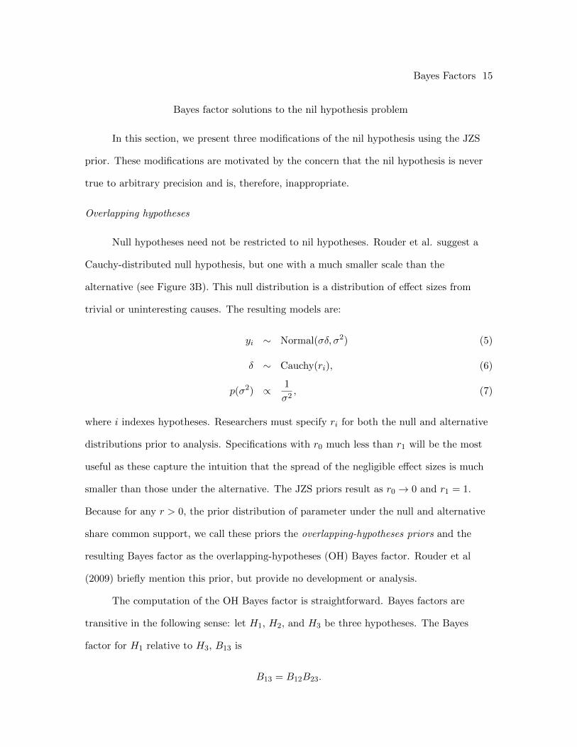
Consequently, the Bayes factor converges in the large sample limit to a finite nonzero
value. The dotted line in Figure 4 shows this behavior for the case that true δ = 1,
r0 = 0.1 and r1 = 1. The lines represent the Bayes factors for the median t value that will
be observed for an effect size δ = 1 as sample size grows. The OH Bayes factor approaches
Bayes Factors 17
the ratio of the prior densities at δ = 1. In contrast, the JZS Bayes factor converges to
BF01 = 0, indicating that increasing the sample size will eventually lead to one
hypothesis, or the other, with certainty.
This undesirable limiting behavior of the OH Bayes factor is a direct consequence of
the fact that the hypotheses were constructed as overlapping hypotheses. Any given effect
size corresponds, to some extent, with both hypotheses. The ambiguity of true effect sizes
relative to the hypotheses is undesirable. To mitigate this problem, we develop hypotheses
that have exclusive support.
Non-overlapping hypotheses
The OH Bayes factor has properties that make it unsuitable for inference. The same
true effect size could be considered null, or not null, depending on whether it came from
the null or alternative distribution. This interpretability problem, along with the
consequence that the Bayes factor does not converge to either 0 or ∞, motivates the
development of a Bayes factor in which the null and alternative are mutually exclusive
ranges of values. We specify a set of priors that are non-overlapping and derive the
corresponding non-overlapping (NOH) Bayes factor as follows. To begin, consider the
model:
yi ∼ Normal(σδ,σ2) (8)
δ ∼ t(ν0) (9)
p(σ2) ∝ 1
σ2. (10)
In this case, the model has been slightly modified so that the distribution on δ is t rather
than scaled Cauchy. The researcher must choose a value for ν0, the degrees of the t
distribution. Setting ν0 = 1 yields the JZS Cauchy prior; setting ν0 = ∞ yields a standard
normal prior (the unit-information prior of Rouder et al., 2009). This generalization
allows the model to subsume the two models suggested by Rouder et al.

Bayes Factors 18
The null hypothesis H2 for the nonoverlapping (NOH) Bayes Factor is that the
effect size δ is within some range (−c, c) of 0. The alternative H3 is that the effect size is
not within this range.
H2 : δ ∼ t(ν0), δ ∈ (−c, c)
H3 : δ ∼ t(ν0), δ /∈ (−c, c)
The NOH Bayes Factor B23 is
B23 =
∫δ∈∆2
∫λ2(λ2)−
N2 −1 exp
{−N−1
2λ2 − 12λ2
(t− δ
√Nλ2
)2}(
1 + (δ/r)2
ν0
)− ν0+12
dλ2dδ
∫δ∈∆3
∫λ2(λ2)−
N2 −1 exp
{−N−1
2λ2 − 12λ2
(t− δ
√Nλ2
)2}(
1 + (δ/r)2
ν0
)− ν0+12
dλ2dδ
× 1− π2π2
where ∆2 is the null region, and ∆3 is the complement of ∆2. The derivation of this
formula is shown in the appendix. To compute the Bayes factor B23 requires 3 integrals:
first, the integration with respect to λ2, then the integration with respect to δ for each
hypothesis. A closed form expression for the Bayes factor is not available, but the
integrals may be performed numerically. We discuss methods of computing this integral in
the appendix, and provide a convenient web applet for computing Bayes factors at
http://pcl.missouri.edu/bayesfactor.
Like the JZS Bayes Factor B01, the NOH Bayes Factor B23 is a function of only the
observed t and the sample size N . The researcher must supply the bounds of the null
hypotheses region (−c, c); this will be discussed later. Following Cohen’s suggestion
(Cohen, 1988) that 0.2 is a “small” effect size, our examples all use a null region of (-0.2,
0.2).
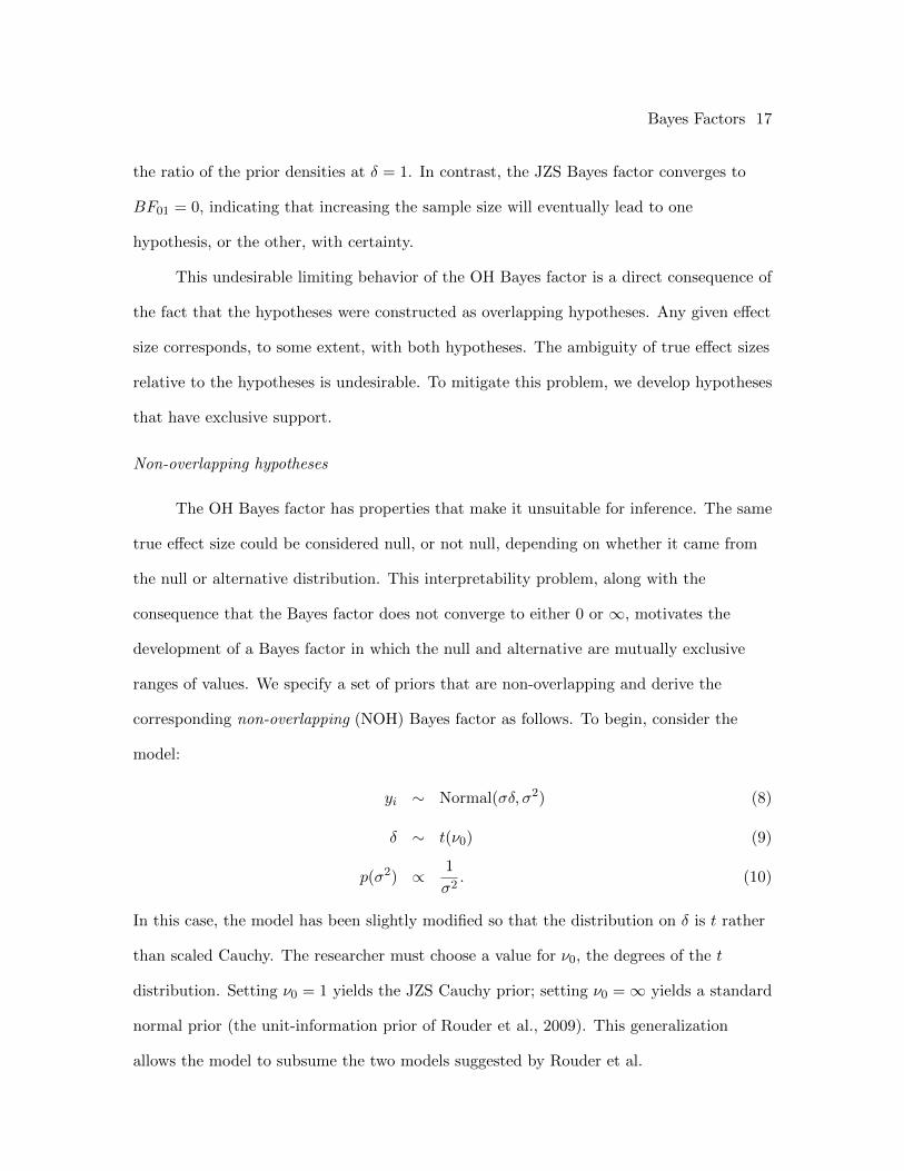
Figure 5 shows the NOH Bayes factor for the median observed t value for several
sample sizes and true effect sizes. The Bayes factor converges to the correct hypothesis for
all hypotheses except when the true effect sizes is exactly on a boundary (-0.2 and 0.2). In

Bayes Factors 19
this case, the Bayes factor converges a finite constant which depends on the prior
distributions, because the data cannot differentiate between the two hypotheses. The
figure includes the NOH Bayes factor for the two extreme values of ν0, 1 and ∞,
corresponding respectively to a standard Cauchy prior and standard normal prior on δ.
The Cauchy prior marginally favors the null hypothesis, due to the heavier weighting of
larger effect sizes, but both priors lead to substantially the same result.
As a comparison to the JZS and OH Bayes factor, we return to the data of Grider
and Malmburg (2008). Recall that the observed t(79) was 2.24, and the observed effect
size was δ = 0.25. Because the effect size is near the null effect range, we expect the NOH
Bayes factor to be more favorable to the null hypothesis than the other two Bayes factors.
Indeed, B23 = 3.63 indicating that the data show a reasonable amount of evidence for the
hypothesis that the true effect size is within (−0.2, 0.2). Whether Grider and Malmburg
would consider all null hypotheses in this interval to be negligible is not known, but the
Bayes factor nevertheless indicates that whatever effect exists is likely to be small.
A hybrid model
Previously, we have argued that (a) the nil point-null hypothesis is unlikely, and
perhaps impossible, and (b) there is a range of effect sizes around the nil hypothesis that,
from the researcher’s perspective, should be treated as null. If we accept (a), then (b)
naturally follows. However, we may accept (b) but deny (a): the two claims need not be
accepted together. This fact motivates the following generalization of the NOH null.
Consider the mixture model for the null shown in Figure 3D. Like the JZS point-null
model, there is point mass at δ = 0. However, like the NOH null model, small effect sizes
around the nil hypothesis are also considered null. We call this model the hybrid null
model. Let π0 be the mixing probability; π0 = 1 corresponds to the case where the null
mixture consists solely of the JZS null and π0 = 0 corresponds to the case where the null

Bayes Factors 20
mixture consists solely of the NOH null.
We call the associated Bayes factor the hybrid Bayes factor and denote it B(02)3 to
indicate that the null is the mixture of H0 (the nil) and H2 (δ ∈ (−c, c)) while the
alternative is H3 (δ /∈ (−c, c)):
B(02)3 =P (Y |H0 or H2)
P (Y |H3).
Computation of B(02)3 is relatively straightforward. Because H0 and H2 are
mutually exclusive, the hybrid Bayes factor may be written
B(02)3 =π0P (Y |H0) + (1− π0)P (Y |H2)
P (Y |H3)
where
π0 =P (H0)
P (H0) + P (H2)
The constant π0 acts as a weight that must be determined before the analysis. It
represents the analyst’s prior beliefs about the proportion of null hypotheses that are nil.
Because the hypotheses H2 and H3 together are the same as the alternative H1 of the JZS
Bayes factor,
P (Y |H1) = π2P (Y |H2) + (1− π2)P (Y |H3)
Using the above facts, algebraic rearrangement yields
B(02)3 = π0B01(π2B23 − π2 + 1) +B23(1− π0), (11)
where
B01 =P (Y |H0)
P (Y |H1)
B23 =P (Y |H2)
P (Y |H3)
Thus, the hybrid Bayes factor B(02)3 is only a function of the point-null Bayes factor, the
corresponding NOH Bayes factor, and the mixing probability π0.
Bayes Factors 21
The hybrid Bayes factor model may appear unusual at first glance. However, it has
some interesting properties that make it an attractive model for inference. First, it is a
generalization of both the JZS Bayes factor and the NOH Bayes factor. With c → 0, the
JZS Bayes factor is obtained. With π0 → 0, the NOH Bayes factor is obtained.
Parameters of the hybrid model may be manipulated to obtain other interesting models as
well, including tests of ordinal hypotheses to be discussed later.
Another interesting feature of the hybrid model can be seen by setting π0 = 1. This
model is shown in Figure 7A. The model represents the situation where the researcher
wants to ignore small effect sizes in testing a nil hypothesis. This is a direct test of
“reasonable” effect sizes against the nil. Figure 7B shows the corresponding hybrid Bayes
factor, which we call the notched Bayes factor. Johnson and Rossell (2010) proposed
similar priors on the alternative hypothesis for computing Bayes factors, arguing that these
priors balance the rates of evidence accumulation for the nil and the alternative. This can
be easily seen by comparing the rate of evidence accumulation for the nil hypothesis of the
JZS Bayes factor to the rate of accumulation of the hybrid Bayes factor in Figure 7B. The
notched Bayes factor follows the JZS Bayes factor fairly closely for moderate to large
effect sizes, but accumulates evidence for the nil more quickly for small effect sizes.
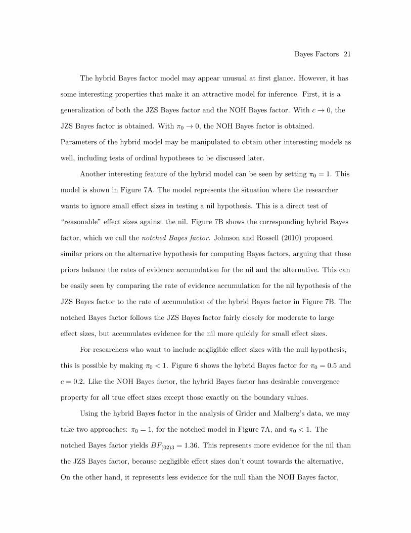
For researchers who want to include negligible effect sizes with the null hypothesis,
this is possible by making π0 < 1. Figure 6 shows the hybrid Bayes factor for π0 = 0.5 and
c = 0.2. Like the NOH Bayes factor, the hybrid Bayes factor has desirable convergence
property for all true effect sizes except those exactly on the boundary values.
Using the hybrid Bayes factor in the analysis of Grider and Malberg’s data, we may
take two approaches: π0 = 1, for the notched model in Figure 7A, and π0 < 1. The
notched Bayes factor yields BF(02)3 = 1.36. This represents more evidence for the nil than
the JZS Bayes factor, because negligible effect sizes don’t count towards the alternative.
On the other hand, it represents less evidence for the null than the NOH Bayes factor,
Bayes Factors 22
because negligible effect sizes don’t count towards the null.
We can also compute the Bayes factor with both a point-null and an interval null.
With π0 = 0.5, we obtain a hybrid Bayes factor BF(02)3 = 2.50. Because the hybrid Bayes
factor includes effect sizes around the nil as evidence for the null hypothesis, this hybrid
Bayes factor indicates more evidence for the null hypothesis than the JZS Bayes factor.
Because it contains a point-null, it is indicates less evidence for the null than the NOH
Bayes factor.
Extensions to Ordinal Constraint
The preceding development focused on testing theories that predict equality
constraints. Some theories, however, predict only an ordering of covariate effects. In
general, Bayes factor is well-suited for assessing these ordinal constraints, and the Bayes
factor priors discussed previously may be extended in a straightforward manner.
Consider a researcher whose theory predicts a positive effect. If we assume that
small negligible effects may be found, even when the theory is false (Meehl, 1978), then it
is appropriate to set a lower limit on positive effects. For example, a researcher may
consider all effects above 0.2 as concordant with the hypothesis and all those below .2 as
inconcordant. Using standard NHST terminology, we call δ < .2 the null hypothesis (H0)
and the researcher’s hypothesis, δ ≥ .2, the alternative (H1), although the terms are
arbitrary in this case. Note that in this setup, negative effects are considered plausible
under the null. The computation of this one-sided Bayes factor is a straightforward
extension of the previous development. The one-sided Bayes factor is equivalent to the
NOH Bayes factor with a null region of (−∞, c). All other details remain the same. We
provide an applet to compute this one-sided Bayes factor at
http://pcl.missouri.edu/bayesfactor, and software at
http://drsmorey.org/research/rdmorey.

Bayes Factors 23
The value of this one-sided Bayes factor for the Grider and Malberg data is 0.41.
When the Bayes factor is less than 1.0, it is often more convenient to report the reciprocal
and the favored hypothesis, which in this case is about 2.46 in favor of the the alternative.
The Bayes factor indicates that the data slightly favor a medium or large positive effect
over a negative or small positive one.
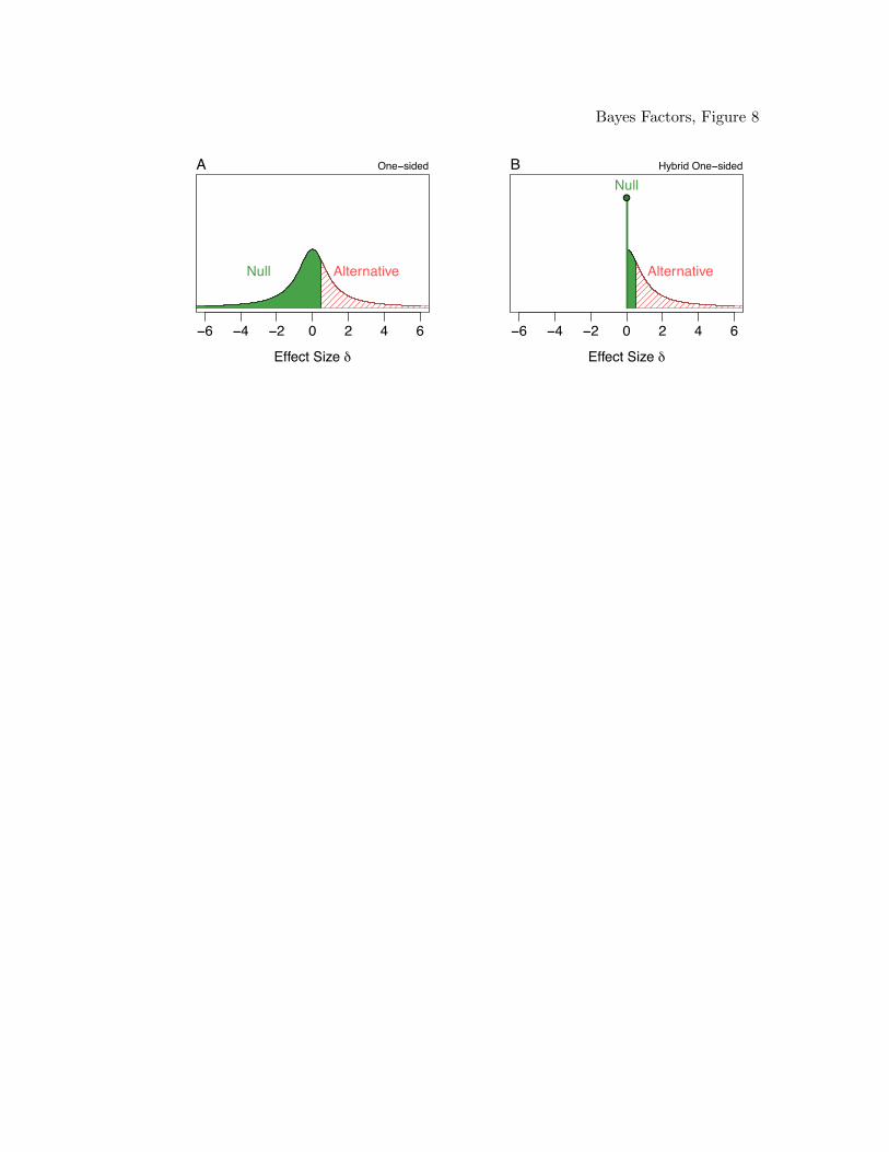
The one-sided hypothesis in the the left panel of Figure 8 assumes a rather flexible
null hypothesis that can includes large negative effects as well as near equalities. In many
cases, large negative effect sizes may be considered unreasonable or uninteresting a priori.
If negative effects are unreasonable or uninteresting, it is possible to eliminate them from
the test, because the Bayes factor will penalize the null hypothesis for the flexibility added
by the range of negative values. The right panel of Figure 8 shows the researcher’s
hypothesis as the alternative against a hybrid null consisting of a mixture between a point
nil at 0 and a region of unimportant positive effect sizes. This extension of the hybrid null
allows the researcher to test their hypothesis against the hypothesis that the effect is
unimportant and positive, or 0. This Bayes factor is reasonable when negative effects are
unreasonable a priori.
To compute the hybrid one-sided Bayes factor, we again relax the assumption of a
symmetric null region. First, we compute the hybrid Bayes factor of the nil versus all
positive values of δ, by setting the null region to (−∞, 0) and π0 = 1, and call this B1.
This yields the one-sided test of Wetzels et al. (2009). We then compute the Bayes NOH
Bayes factor B2, with null region (0, c) and alternative region (c,∞). The hybrid
one-sided Bayes factor may then be computed by applying Eq. 11.
Applying the hybrid one-sided Bayes factor with π0 = 0.5 and π0 = 1 to Grider and
Malberg’s data yields Bayes factors of 1.91 for the null, and 1.7 for the alternative,
respectively. Both of these Bayes factor values are concordant with the other Bayes factor
values computed in this paper, suggesting that the data have little evidentiary value.
Bayes Factors 24
Discussion
In this paper we developed Bayes factors for testing equality and ordinal
constraints. Our advocacy of Bayes factor is based on the concept of evidence, namely
that researchers may consider it helpful to report the evidence in data for various
positions than make decisions with specified error rates. The Bayes factor is the marginal
probability of the data under two competing hypotheses, and this ratio is directly
interpretable without recourse to decision regions or error rates. It is possible to use Bayes
factors to compute quantities that are appropriate for decision-making, if desired.
Posterior odds reflect an analyst’s belief about the relative weighting of two hypotheses
given observed data and are a thus a natural quantity for making decisions. We find both
posterior odds and Bayes factor directly interpretable, though we prefer Bayes factor for
scientific communication. Some researchers, however, may argue that posterior odds are
more interpretable than Bayes factors. For example, there are Bayesian statistical
equivalence tests based on posterior odds rather than Bayes factor (e.g., Selwyn,
Dempster & Hall, 1981; Selwyn & Hall, 1984; Wellek, 2003). In fact, these tests are based
on improper priors in which the prior odds and Bayes factors cannot be meaningfully
defined. We view these approaches, in which one cannot quantify the amount of evidence
contributed by the data, as less advantageous.
Researchers who prefer posterior odds to Bayes factors may still use our methods;
they must, however, stipulate prior odds. Prior odds may be used to add context to an
analysis; if a hypothesis is highly unlikely a prior, it may be assigned low prior odds. One
example is Bem’s (in press) recent claim that participants can sense random events before
they occur, or precognition. We recently analyzed Bem’s claims, and found that the Bayes
factor computed from Dr. Bem’s reported data was 40 in favor of ESP (Rouder and
Morey, submitted). While this Bayes factor is large, we cautioned readers to use very
unfavorable prior odds in interpreting the results because precognition is contrary to
Bayes Factors 25
well-established laws and principles in physics and biology. If one begins with extremely
low prior odds for a hypothesis, more evidence will be necessary. This strikes us as both
reasonable and a reflection of how scientists reason; quantifying of this reasoning whenever
possible will make the scientific process appropriately responsive to evidence. Prior odds
are therefore useful for adding context to a Bayes factor; however, due to its insensitivity
to prior odds, we recommend reporting of Bayes factor; computing posterior odds is then
simply a matter of multiplication, as can easily be seen in Eq. 4.
Bayes factor, the ratio of marginal probabilities, is contingent on specification of a
prior over parameters under competing hypotheses. We have presented a number of
different specifications for nulls and alternatives. Researcher interested in these techniques
my wonder which of the several null and alternatives they should use. Consider first the
question of assessing equality constraints. Our recommendation is the hybrid setup in
Figure 3D. This hybrid model is quite general and seems highly appropriate under many
conditions. We provide an easy-to-use web applet that calculates hybrid Bayes factors at
http://pcl.missouri.edu/bayesfactor, shown in Figure 9. For ordinal tests, we recommend
either Bayes factor in Figure 8 for assessing ordinal constraints, depending on whether the
researcher believes negative effects are reasonable a priori. Moreover, as previously
discussed, in Bayesian statistics, there is no drawback to computing and reporting
multiple tests.
Once a test is selected, researchers must also choose model parameters, such as
equivalence regions or the weight parameter π0. Choices of the equivalence regions and
weights of the point nil reflect reasoned beliefs about the problem at hand. In fields where
interesting effects are smaller (for example, subliminal priming), the width of the null
region may be made correspondingly small. In other fields where interesting effect sizes
are larger (for example, cognitive aging), the region may be made larger to suit. The task
of selecting boundaries is simplified somewhat by the parameterization. The models are
Bayes Factors 26
parameterized with respect to standardized effect size. General guidelines already exist
(Cohen, 1988) and we note that many journals require reporting some measure of effect
size. Certainly if researchers are able to interpret effect size measures in the context of
existing literature, it is not difficult to extend this to setting bounds on equivalence
regions. Eventually conventions may arise, as they have with type I error rate. However,
because these Bayes factors are computed using only the t test statistic and sample size,
any researcher may calculate a Bayes factor for themselves, using a different equivalence
region.
In addition to specifying equivalence regions, computing the hybrid Bayes Factor
requires specifying the mixture probability that null hypotheses are nil, π0. The value of
π0 will depend on the type of test desired. For researchers who believe that nil hypotheses
are impossible a priori, or who are uninterested in the nil, π0 = 0 is a reasonable value.
For researchers who want to test nil hypotheses against reasonable, nonnegligible values of
δ, we recommend π0 = 1 with an null interval including negligible effect sizes (Figure 7A).
Other values may correspond to other models of interest. Setting π0 should pose no great
difficulty for researchers. If researchers report their test statistics, other researchers will be
able to reproduce the analysis with different values, if desired. In all cases, however, the
interpretation of Bayes factors should be understood in the context of the assumptions
about the equivalence regions and π0, and not as assumption-free measures of evidence.
It should also be noted that in spite of the wide range of models employed in this
paper to compute Bayes factors, in the example using Grider and Malmberg’s data, the
Bayes factor ranged from about 2.7 for an effect, to 3.6 against, all indicating that there is
little or no evidence for a substantial effect. It is not surprising that the Bayes factors
vary, because the null hypothesis tested was in each case different: some were point
hypothesis, some ranges of values, and some mixtures of the two. But the interpretation of
the Bayes factor with respect to the hypothesis in question, whether we should take the
Bayes Factors 27
experiment as evidence of an effect, is substantially the same.
Conclusion
We have presented here a Bayes factor approach to hypothesis testing that has the
following advantages: first, it allows for null hypotheses that are not exactly nil. In this
way, small, uninteresting effects are not emphasized. Second, the use of Bayes factors
allows for the accumulation of evidence for both the null and the alternative hypotheses
simultaneously. Third, because the Bayes factor is a relative measure, it does not
overstate the evidence against a default hypothesis. Fourth, the framework suggested is
sufficiently general to construct tests of equivalence and ordinal tests. The key innovation
in these Bayes factors is that they allow researchers to accept a theoretically meaningful
constraint even when it fails for trivial or uninteresting reasons, through the use of
equivalence regions. This ability to judiciously quantify the evidence for and against
constraints in real-world situations should lead to better understanding of lawfulness and
parsimony in psychology.
Bayes Factors 28
References
Abramowitz, M., & Stegun, I. A. (1965). Handbook of mathematical functions: with
formulas, graphs, and mathematical tables. New York: Dover.
Bayarri, M. J., & Garcia-Donato, G. (2007). Extending conventional priors for testing
general hypotheses in linear models. Biometrika, 94 , 135-152.
Bem, D. (in press). Feeling the future: Experimental evidence for anamalous retroactive
infleces on cognition and affect. Journal of Personality and Social Psychology .
Berger, J. O., & Delampady, M. (1987). Testing precise hypotheses. Statistical Science,
2 (3), 317-335. Available from http://www.jstor.org/pss/2245772
Berger, J. O., & Sellke, T. (1987). Testing a point null hypothesis: The irreconcilability of
p values and evidence. Journal of the American Statistical Association, 82 (397),
112–122. Available from http://www.jstor.org/stable/2289131
Berkson, J. (1938). Some difficulties of interpretation encountered in the application of
the chi-square test. Journal of the American Statistical Association, 33 (203),
526-536. Available from http://www.jstor.org/stable/2279690
Bernardo, J. M., & Smith, A. F. M. (2000). Bayesian theory. Chichester, England: John
Wiley & Sons.
Cohen, J. (1988). Statistical power analysis for the behavioral sciences (2nd ed.).
Hillsdale, NJ: Erlbaum.
Cohen, J. (1994). The earth is round (p < .05). American Psychologist , 49 , 997-1003.
Cox, R. T. (1946). Probability, frequency and reasonable expectation. American Journal
of Physics, 14 , 1–13.
De Finetti, B. (1992). Probability, induction and statistics : the art of guessing. Wiley.
Dougal, S., & Rotello, C. M. (2007). “remembering” emotional words is based on response
bias, not recollection. Psychonomic Bulletin & Review , 14 , 423-429.
Gelman, A., Carlin, J. B., Stern, H. S., & Rubin, D. B. (2004). Bayesian data analysis
Bayes Factors 29
(2nd edition). London: Chapman and Hall.
Green, D. M., & Swets, J. A. (1966). Signal detection theory and psychophysics. New
York: Wiley. Reprinted by Krieger, Huntington, N.Y., 1974.
Grider, R. C., & Malmberg, K. J. (2008). Discriminating between changes in bias and
changes in accuracy for recognition memory of emotional stimuli. Memory &
Cognition, 36 , 933-946.
Hacking, I. (1965). Logic of statistical inference. Cambridge, England: Cambridge
University Press.
Hodges, J., J. L., & Lehmann, E. L. (1954). Testing the approximate validity of statistical
hypotheses. Journal of the Royal Statistical Society. Series B (Methodological),
16 (2), 261–268. Available from http://www.jstor.org/stable/2984052
Iverson, G. J., Lee, M. D., & Wagenmakers, E. J. (2009). prep misestimates the
probability of replication. Psychonomic Bulletin and Review , 16 (424-429).
Jaynes, E. (1986). Bayesian methods: General background. In J. Justice (Ed.),
Maximum-entropy and bayesian methods in applied statistics. Cambridge:
Cambridge University Press.
Jeffreys, H. (1946). An invariant form for the prior probability in estimation problems.
Proceedings of the Royal Society of London. Series A, Mathematical and Physical
Sciences, 186 (1007), 453–461. Available from
http://www.jstor.org/stable/97883
Jeffreys, H. (1961). Theory of probability (3rd edition). New York: Oxford University
Press.
Johnson, V. E., & Rossell, D. (2010). On the use of non-local prior desities in Bayesian
hypothesis tests. Journal of the Royal Statistical Society, Series B , 72 , 143–170.
Kass, R., & Raftery, A. (1995). Bayes factors. Journal of the American Statistical
Association, 90 , 773-795. Available from http://www.jstor.org/stable/2291091

Bayes Factors 30
Laplace, P. S. (1986). Memoir on the probability of the causes of events. Statistical
Science, 1 (3), 364–378. Available from http://www.jstor.org/stable/2245476
Luce, R. D. (1963). Detection and recognition. In R. D. Luce, R. R. Bush, & E. Galanter
(Eds.), Handbook of mathematical psychology (vol. 1). New York: Wiley.
Meehl, P. E. (1978). Theoretical risks and tabular asterisks: Sir Karl, Sir Ronald, and the
slow progress of soft psychology. Journal of Consulting and Clinical Psychology,, 46 ,
806–834. Available from
http://www.psych.umn.edu/faculty/meehlp/113TheoreticalRisks.pdf
Murphy, N. A., & Isaacowitz, D. M. (2008). Preferences for emotional information in
older and younger adults: A meta-analysis of memory and attention tasks.
Psychology and Aging , 23 , 263–286.
Press, W. H., Teukolsky, S. A., Vetterling, W. T., & Flannery, F. P. (1992). Numerical
recipes in C: The art of scientific computing. 2nd ed. Cambridge, England:
Cambridge University Press.
Rogers, J. L., Howard, K. I., & Vessey, J. T. (1993). Using significance tests to evaluate
the equivalence between two experimental groups. Psychological Bulletin, 113 ,
553-565.
Rouder, J. N., & Morey, R. D. (n.d.). An assessment of the evidence for feeling the future
with a discussion of bayes factor and significance testing.
Rouder, J. N., Speckman, P. L., Sun, D., Morey, R. D., & Iverson, G. (2009). Bayesian
t-tests for accepting and rejecting the null hypothesis. Psychonomic Bulletin and
Review , 16 , 225-237.
Royall, R. (1997). Statistical evidence: A likelihood paradigm. New York: CRC Press.
Rozeboom, W. W. (1960). The fallacy of the null-hypothesis significance test.
Psychological Bulletin, 57 , 416-428. Available from
http://psychclassics.yorku.ca/Rozeboom/

Bayes Factors 31
Sellke, T., Bayarri, M. J., & Berger, J. O. (2001). Calibration of p values for testing
precise null hypotheses. American Statistician, 55 , 62-71. Available from
http://www.jstor.org/stable/2685531
Selwyn, M. R., Dempster, A. P., & Hall, N. R. (1981). A Bayesian approach to
bioequivalence for the 2 x 2 changeover design. Biometrics, 37 (1), 11–21. Available
from http://www.jstor.org/stable/2530518
Selwyn, Murray R., & Hall, Nancy R. (1984). On Bayesian methods for bioequivalence.
Biometrics, 40 (4), 1103–1108. Available from
http://www.jstor.org/stable/2531161
Shibley Hyde, J. (2005). The gender similarities hypothesis. American Psychologist , 60 ,
581-592.
Shibley Hyde, J. (2007). New directions in the study of gender similarities and differences.
Current Directions in Psychological Science, 15 , 259-263.
Sternberg, S. (1969). The discovery of prossesing stages: Extensions of Donder’s method.
In W. G. Kosner (Ed.), Attention and performance ii. Amsterdam: North-Holland.
Thapar, A., & Rouder, J. (2009). Aging and recognition memory for emotional words: A
bias account. Psychonomic Bulletin & Review , 16 , 699-704.
Wagenmakers, E.-J. (2007). A practical solution to the pervasive problem of p values.
Psychonomic Bulletin and Review , 14 , 779-804.
Wagenmakers, E.-J., Lee, M. D., Lodewyckx, T., & Iverson, G. (2008). Bayesian versus
frequentist inference. In H. Hoijtink, I. Klugkist, & P. Boelen (Eds.), Practical
Bayesian approaches to testing behavioral and social science hypotheses (p. 181-207).
New York: Springer.
Wellek, S. (2003). Testing statistical hypotheses of equivalence. Boca Raton: Chapman &
Hall/CRC.
Wetzels, R., Raaijmakers, J. G. W., Jakab, E., & Wagenmakers, E.-J. (2009). How to
Bayes Factors 32
quantify support for and against the null hypothesis: A flexible WinBUGS
implementation of a default Bayesian ttest. Psychonomic Bulletin & Review , 16 ,
752-760.
Zellner, A., & Siow, A. (1980). Posterior odds ratios for selected regression hypotheses. In
J. M. Bernardo, M. H. DeGroot, D. V. Lindley, & A. F. M. Smith (Eds.), Bayesian
statistics: Proceedings of the First International Meeting held in Valencia (Spain)
(pp. 585–603). University of Valencia.

Bayes Factors 33
Appendix A
Derivation of Nonoverlapping Bayes Factor
The joint prior p2 on δ and σ2 for hypothesis H2 is
p2(δ,σ2) =
1
π2σ2tν0,r(δ)I(δ ∈ ∆2)
where tν0,r is the density function of the central t distribution with ν0 degrees of freedom
and scale r, I is an indicator function, ∆2 is the null region (−c, c), and
π2 =
∫ c
−ctν0,r(δ)dδ
Similarly, the joint prior for H3 is
p3(δ,σ2) =
1
(1− π2)σ2tν0,r(δ)I(δ /∈ ∆2)
The NOH Bayes factor is the ratio of the marginal likelihoods,
B23 =
∫
δ∈∆2
∫
σ2p(Y |σ2, δ)p2(δ,σ
2)dδσ2
/ ∫
δ∈∆2
∫
σ2p(Y |σ2, δ)p3(δ,σ
2)dδ, dσ2(12)
To find a complete expression of the Bayes Factor, we first consider the joint
posterior of δ and σ2:
p(δ,σ2|Y ) ∝ 1
π2(σ2)−
N2 exp
{− 1
2σ2
∑
i
(yi − σδ)2}(σ2)−1
(1 +
(δ/r)2
ν0
)− ν0+12
(13)
The constants with respect to σ2 and δ can be safely ignored, because the will be the
same for both the numerator and the denominator in Eq. 12. Expanding the square and
distributing the sum yields
p(δ,σ2|y) ∝ 1
π2(σ2)−
N2 exp
{− 1
2σ2
(∑
i
y2i − 2σδNY +Nσ2δ2)}
(σ2)−1
(1 +
(δ/r)2
ν0
)− ν0+12
Using the identity∑
i y2i = (N − 1)s2 +Ny2,
p(δ,σ2|y) ∝ 1
π2(σ2)−
N2 exp
{− 1
2σ2
((N − 1)s2 +NY 2 − 2σδNY +Nδ2σ2
)}

Bayes Factors 34
×(σ2)−1
(1 +
(δ/r)2
ν0
)− ν0+12
∝ (σ2)−N2 exp
{− s2
2σ2
((N − 1) +
NY 2
s2− 2
σδNY
s2+
Nσ2δ2
s2
)}
×(σ2)−1
(1 +
(δ/r)2
ν0
)− ν0+12
∝ 1
π2(σ2)−
N2
× exp
{− 1
2σ2/s2
((N − 1) +
NY 2
s2− 2
√Nδ
σ
s
√NY
s+Nδ2
σ2
s2
)}
×(σ2)−1
(1 +
(δ/r)2
ν0
)− ν0+12
We can substitute the following notation:
t =Y
s/√N
λ2 =σ2
s2
The substitution yields
p(δ,σ2|y) ∝ 1
π2(λ2)−
N2 (s2)−
N2 exp
{−N − 1
2λ2
}
× exp
{− 1
2λ2
(t2 − 2
√Nδλ2t+Nδ2λ2
)}
×(λ2)−1(s2)−1
(1 +
(δ/r)2
ν0
)− ν0+12
∝ 1
π2(λ2)−
N2 −1 exp
{−N − 1
2λ2
}
× exp
{− 1
2λ2
(t− δ
√Nλ2
)2}
×(1 +
(δ/r)2
ν0
)− ν0+12
After a similar simplification for H3, the NOH Bayes Factor is
B23 =
∫δ∈∆2
∫λ2(λ2)−
N2 −1 exp
{−N−1
2λ2 − 12λ2
(t− δ
√Nλ2
)2}(
1 + (δ/r)2
ν0
)− ν0+12
dλ2dδ
∫δ∈∆3
∫λ2(λ2)−
N2 −1 exp
{−N−1
2λ2 − 12λ2
(t− δ
√Nλ2
)2}(
1 + (δ/r)2
ν0
)− ν0+12
dλ2dδ
× 1− π2π2
where ∆3 is the complement of ∆2.

Bayes Factors 35
Appendix B
Approaches to computing the Bayes factor
One standard approach to numerical integration is Gaussian quadrature
(Abramowitz & Stegun, 1965; Press, Flannery, Teukolsky, & Vetterling, 1988), which is
implemented in many software packages including Matlab and R. We have found that
Gaussian quadrature integration is very quick in practice, but can be unstable in
circumstances where the posterior mass is highly concentrated over a small interval.
A second approach is using Normal approximations to the marginal posterior
distribution of δ. As before, Gaussian quadrature may be used to integrate out σ2,
yielding the marginal posterior on δ. For reasonable sample sizes, the marginal posterior
will be approximately Normally distributed (Bernardo & Smith, 2000). Laplace’s method
(Laplace, 1774/1986) approximates an integral using the normal distribution function,
leading to a highly accurate approximation for the integral and thus the posterior odds.
The prior odds may be computed easily by standard statistical software. In cases where
Gaussian quadrature fails, Laplace’s method may be used to compute the NOH Bayes
factor quickly and accurately.

Bayes Factors 36
Author Note
Richard D. Morey, Faculty of Behavioral and Social Sciences, University of
Groningen; Jeffrey N. Rouder, Department of Psychological Sciences, University of
Missouri.
Address correspondence to Richard D. Morey, Psychometrics and Statistics, Grote
Kruisstraat 2/1, Groningen, the Netherlands, email: [email protected].

Bayes Factors 37
Footnotes
1A point hypothesis on a parameter takes the form θ = c The hypothesis may be
rewritten as θ′ = 0, where θ′ = θ − c.
2The distribution function of normal distribution with mean µ and variance σ2 is
φ(y | µ,σ2) = (2πσ2)− 1
2 exp
{− (y−µ)2
2σ2
}
3Consistency can be obtained in conventional NHST if the type I error rate is
reduced to zero with increasing sample size, but this is not done in practice and to our
knowledge no one has proposed a way of doing so.
Bayes Factors 38
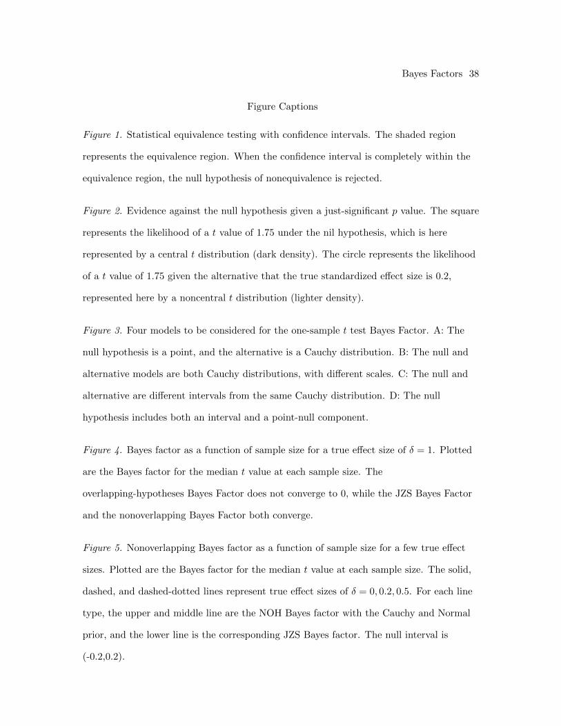
Figure Captions
Figure 1. Statistical equivalence testing with confidence intervals. The shaded region
represents the equivalence region. When the confidence interval is completely within the
equivalence region, the null hypothesis of nonequivalence is rejected.
Figure 2. Evidence against the null hypothesis given a just-significant p value. The square
represents the likelihood of a t value of 1.75 under the nil hypothesis, which is here
represented by a central t distribution (dark density). The circle represents the likelihood
of a t value of 1.75 given the alternative that the true standardized effect size is 0.2,
represented here by a noncentral t distribution (lighter density).
Figure 3. Four models to be considered for the one-sample t test Bayes Factor. A: The
null hypothesis is a point, and the alternative is a Cauchy distribution. B: The null and
alternative models are both Cauchy distributions, with different scales. C: The null and
alternative are different intervals from the same Cauchy distribution. D: The null
hypothesis includes both an interval and a point-null component.
Figure 4. Bayes factor as a function of sample size for a true effect size of δ = 1. Plotted
are the Bayes factor for the median t value at each sample size. The
overlapping-hypotheses Bayes Factor does not converge to 0, while the JZS Bayes Factor
and the nonoverlapping Bayes Factor both converge.
Figure 5. Nonoverlapping Bayes factor as a function of sample size for a few true effect
sizes. Plotted are the Bayes factor for the median t value at each sample size. The solid,
dashed, and dashed-dotted lines represent true effect sizes of δ = 0, 0.2, 0.5. For each line
type, the upper and middle line are the NOH Bayes factor with the Cauchy and Normal
prior, and the lower line is the corresponding JZS Bayes factor. The null interval is
(-0.2,0.2).

Bayes Factors 39
Figure 6. Hybrid Bayes factor as a function of sample size for a few true effect sizes.
Plotted are the Bayes factor for the median t value at each sample size. The solid, dashed,
and dashed-dotted lines represent true effect sizes of δ = 0, 0.2, 0.5. For each line type, the
upper and middle line are the NOH Bayes factor with the Cauchy and Normal prior, and
the lower line is the corresponding JZS Bayes factor. The null hypothesis has mixing
probability π0 = 0.5 and extends on the interval (−.2, .2).
Figure 7. A: The hybrid model with π0 = 1. There is an interval of small effect sizes
which cannot occur under either hypothesis. B: Bayes factor as a function of sample size
for a few true effect sizes. Plotted are the Bayes factor for the median t value at each
sample size. The solid, dashed, and dashed-dotted lines represent true effect sizes of
δ = 0, 0.2, 0.5. For each line type, the upper and middle line are the NOH Bayes factor
with the Cauchy and Normal prior, and the lower line is the corresponding JZS Bayes
factor. The null region was (-0.2,0.2) and π0 = 1.
Figure 8. Possible one-sided hypotheses. The left panel shows hypotheses for a test of
important positive effects against all other effects. The right panel shows hypotheses for a
test of important positive effects against either no effect or unimportant positive effects.
Figure 9. The web applet at http://pcl.missouri.edu/bayesfactor for computing area and
hybrid Bayes factors. Users specify the sample size, t value, equivalence region, π0, and
the prior scale. The web applet returns the corresponding Bayes factor.

Bayes Factors, Figure 1
●
●
●
●
Sample
Obs
erve
d (w
ith C
Is)
−0.3
−0.2
−0.1
0.0
0.1
0.2
0.3
A B C D
Bayes Factors, Figure 2
t value
Dens
ity
●Null t distribution
Alternative t distribution
1.0 1.5 2.0 2.5 3.00.0
0.1
0.2
0.3
0.4
0.1 0.05 0.01one−tailed p value

Bayes Factors, Figure 3
Effect Size δδ
−6 −4 −2 0 2 4 6
Standard JZS point nullANull
Alternative
Effect Size δδ
−6 −4 −2 0 2 4 6
Overlapping hypothesesBNull
Alternative
Effect Size δδ
−6 −4 −2 0 2 4 6
Nonoverlapping hypothesesC
Null
AlternativeAlternative
Effect Size δδ
−6 −4 −2 0 2 4 6
HybridD
●
Null
AlternativeAlternative

Bayes Factors, Figure 4
Sample Size
Med
ian
Baye
s Fa
ctor
10 20 30 40 50
True δδ = 1
JZS
NOH
OH1
10−−1
10−−2
10−−3
10−−4
10−−5
10−−6

Bayes Factors, Figure 5
Sample Size
NOH
Baye
s Fa
ctor
5 40 80 160 320
101102103104
1
10−−1
10−−2
10−−3
10−−4
Favors AlternativeFavors Null

Bayes Factors, Figure 6
Sample Size
Hybr
id B
ayes
Fac
tor
ππ0=0.5
5 40 80 160 320
101102103104
1
10−−1
10−−2
10−−3
10−−4
Favors AlternativeFavors Null

Bayes Factors, Figure 7
Effect Size δδ
−6 −4 −2 0 2 4 6
Hybrid, ππ0=1
●
ANull
AlternativeAlternative
Sample SizeNo
tch
Baye
s Fa
ctor
ππ0=1B
5 40 80 160 320
101102103104
1
10−−1
10−−2
10−−3
10−−4
Favors AlternativeFavors Null
Bayes Factors, Figure 8
Effect Size δ
−6 −4 −2 0 2 4 6
One−sidedA
Null Alternative
Effect Size δ
−6 −4 −2 0 2 4 6
Hybrid One−sidedB
●
Null
Alternative

Bayes Factors, Figure 9
Top Related