


Languages
Pages
Legal


Basis of Energy Efficiency Economical and Ecological Approach Method for
Pumping Equipments and Systems
MIRCEA GRIGORIU
Hydraulics and Hydraulic Machineries
University POLITEHNICA Bucharest
313 Spl.Independentei, Bucharest-
ROMANIA
[email protected] http://www.hydrop.pub.ro
Abstract: The paper presents the basis of an original economical and ecological approach of the pumping systems
energy efficiency, offering a holistic picture of the pumping efficiency, with emphasis in economical and GHGs
emissions mitigation effects. The main contributions consists in the original energy efficiency evaluation method of
pumping equipments, a particularization of the pumping systems optimal operation characteristic determination for
variable requested flow conditions, and a practical application for parallel operation variable speed driving adjustment,
the actual most applied system. In the application, there are emphasis economic and environmental effects, with a
special focus on the GHGs emissions. The paper results application consists in automatic driving operation and in new
pumping optimization operation solution evaluation, including pumps and motors energy classification, considering
the actual international trends and European Commission commitments in energy and climate changes fields.
Key-Words: energy efficiency, GHGs emission mitigation, operation modeling, variable speed driving
1. European frame of energy efficiency
innovation
Pumping systems and equipments energy efficiency
improvement is vital in reaching the energy and climate
change European policy objectives: to reduce
greenhouse gas emissions by 20% and ensure 20% of
renewable energy sources in the EU energy mix; to
reduce EU primary energy use by 20% by 2020.
Considering that energy consumption in this type of
installations represents more that 20% of the total energy
consumption of a modern economy, pumping system
efficiency improvement could have a consistent
contribution to the effort to accelerate the development
and deployment of cost-effective low carbon and energy
efficiency technologies. Energy industry has five clear
components (resources, production, transport,
distribution and consumption), each of them with
specific problems and solutions. In the longer term, the
solutions for decarbonizes the economy and improve
energy efficiency, new generations of technologies have
to be developed through breakthrough in research. Since
the oil price shocks in the 70s and 80s, Europe has
enjoyed inexpensive and plentiful energy supplies. The
easy availability of resources, no carbon constraints and
the commercial imperatives of market forces have not
only left the union dependent on fossil fuels, but have
also tempered the interest for innovation and investment
in new energy technologies. This has been described as
the greatest and widest-ranging market failure ever seen.
Intrinsic weaknesses in energy innovation
The energy innovation process, from initial conception
to market penetration, also suffers from unique structural
weaknesses. It is characterized by long lead times, often
decades, to mass market due to the scale of the
investments needed and the technological and regulatory
inertia inherent in existing energy systems. Innovation
faces entrenched 'locked-in' carbon based infrastructure
investments, dominant actors, imposed price caps,
changing regulatory frameworks and network
connection challenges. The market take-up of new
energy technologies is additionally hampered by the
commodity nature of energy. New technologies are
generally more expensive than those they replace while
not providing a better energy service. The immediate
benefits tend to accrue to society rather than the buyers.
Some technologies face social acceptance issues and
often require additional up-front integration costs to fit
into the existing energy system. Legal and
administrative barriers complete this innovation adverse
framework. In short, there is neither a natural market
appetite nor a short-term business benefit for such
technologies. This market gap between supply and
demand is often referred to as the 'valley of death' for
low carbon energy technologies. Public intervention to
support energy innovation is thus both necessary and
justified.
WSEAS TRANSACTIONS on ENVIRONMENT and DEVELOPMENT Mircea Grigoriu
ISSN: 1790-5079 1 Issue 1, Volume 5, January 2009
Between the key EU technological challenges for the
next 10 years to meet the 2020 targets are:
– Bring to mass market more efficient energy conversion
and end-use devices and systems, in buildings, transport
and industry, such as poly-generation and fuel cells;
– Maintain competitiveness in fission technologies,
together with long-term waste management solutions.
And between the Key EU technology challenges for the
next 10 years to meet the 2050 vision is: achieve
breakthroughs in enabling research for energy
efficiency: e.g. materials, nano-science, information and
communication technologies, bio-science and
computation.
Between the European regulations with an important
impact to energy efficiency, are:
- New and unitary Legislation or Amending the
Directive 92/75/EEC-for the global energy and
environmental performance-then-the better and
simplification
- Eco-design: Directive 2005/32/EC of the European
Parliament and of the Council of 6 July 2005,
establishing a framework for the setting of eco-design
requirements for energy-using products and amending
Council Directive 92/42/EEC and Directives 96/57/EC
and 2000/55/EC of the European
Parliament and of the Council
- Energy-Star: Regulation (EC) No. 2422/2001 of the
European Parliament and of the Council of 6 November
2001 on a Community energy efficiency labeling
program for office equipment as amended.
- Energy Labeling: Council Directive 92/75/EEC of 22
September 1992 on the indication by labeling and
standard product information of the consumption of
energy and other resources by household appliances.
- Eco-label: Regulation (EC) No 1980/2000 of the
European Parliament and of the Council of 17 July 2000.
According to the European plans for eco-design
implementation measures, the pumps, funs and electric
motors should be in the phase of drafting measures and
impact assessment by the end of this year.
2. Operation pumps adequate
representation solutions
2.1.Pumps operation point representation
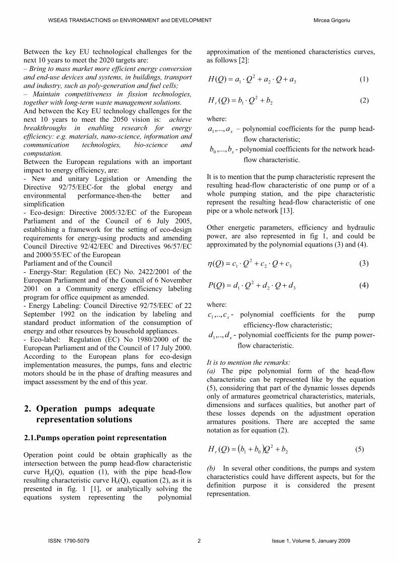
Operation point could be obtain graphically as the
intersection between the pump head-flow characteristic
curve Hp(Q), equation (1), with the pipe head-flow
resulting characteristic curve Hr(Q), equation (2), as it is
presented in fig. 1 [1], or analytically solving the
equations system representing the polynomial
approximation of the mentioned characteristics curves,
as follows [2]:
32
2
1)( aQaQaQH +⋅+⋅= (1)
2
2
1)( bQbQH r +⋅= (2)
where:
xaa ,...,1 – polynomial coefficients for the pump head-
flow characteristic;
xbb ,...,0 - polynomial coefficients for the network head-
flow characteristic.
It is to mention that the pump characteristic represent the
resulting head-flow characteristic of one pump or of a
whole pumping station, and the pipe characteristic
represent the resulting head-flow characteristic of one
pipe or a whole network [13].
Other energetic parameters, efficiency and hydraulic
power, are also represented in fig 1, and could be approximated by the polynomial equations (3) and (4).
32
2
1)( cQcQcQ +⋅+⋅=η (3)
32
2
1)( dQdQdQP +⋅+⋅= (4)
where:
xcc ,..,1 - polynomial coefficients for the pump
efficiency-flow characteristic;
xdd ,..,1 - polynomial coefficients for the pump power-
flow characteristic.
It is to mention the remarks:
(a) The pipe polynomial form of the head-flow
characteristic can be represented like by the equation
(5), considering that part of the dynamic losses depends
only of armatures geometrical characteristics, materials,
dimensions and surfaces qualities, but another part of
these losses depends on the adjustment operation
armatures positions. There are accepted the same
notation as for equation (2).
( ) 2
2
01)( bQbbQH r ++= (5)
(b) In several other conditions, the pumps and system
characteristics could have different aspects, but for the
definition purpose it is considered the present
representation.
WSEAS TRANSACTIONS on ENVIRONMENT and DEVELOPMENT Mircea Grigoriu
ISSN: 1790-5079 2 Issue 1, Volume 5, January 2009

(c) In the picture, the working point is considered the
most efficient operation point of the system. It could be
other operation conditions, characterized by other
parameters, and the pump efficiency could be lower then
the maximum value.
For generalization purposes, in the present paper, all the
pump parameters are represented in non-dimensional
coordinates, defined as follows (6):
( ) ( )
( ) ( )n
x
n
x
n
x
n
x
P
Pp
H
Hh
Q
==
==
%,%'
,%,%
ηη
η (6)
where:
PHQ ,,, η - operation parameters (flow rate, pumping
head, efficiency and hydraulic power);
x - notation for nominal operation parameters;
notation for momentum operation
parameters;
phq ,,, 'η -non-dimensional operation parameters
(flow rate, pumping head, efficiency and
hydraulic power).
2.2.Working point operation adjustment using
variable speed driving solution
If for the maximum efficiency of the pumping
equipments at the nominal working regime is hardly to
obtain significant improvements, taking into
consideration the actual performances of the devices,
there is an important potential to be valuated in pumping
systems operation optimal adjustment.
There are different ways to operate adjustments of
pumps working point, depending to the period of regime
changing, the pumps power and dimensions, pumps and
installation type, adjustment sharpness, etc.
For definitive operation point changing, it is preferable
to action on the pump itself, by using different types of
impellers in the same casing, the same impeller in
different casings, or providing a permanent changing to
a standard pump type.
For operating point changing for a long period of time,
it could be used different types of diaphragms at the
pump outlet or in appropriate points of the network.
For short term changes, it is preferable to use special
adjustable devices of the installation (vanes, by passes),
of the driving engines (variable speed motors), or pump
itself (adjustable impellers for axial flow pumps, or
same diagonal pumps).
Generally, the challenge is between adjustable vanes and
variable speed motors for shot term changes in the
majority types of installations.
For variable speed driving motor and using the same
notations, the pump polynomial form of parameters
characteristics become: head-flow characteristic - (7),
Efficiency-flow characteristic – (8), power-flow
characteristic – (9).
65
4
2
32
2
1),(
aNa
QaNaNQaQaNQH p
+⋅+
+⋅+⋅+⋅⋅+⋅=
(7)
65
4
2
32
2
1),(
cNc
QcNcNQcQcNQ
+⋅+
+⋅+⋅+⋅⋅+⋅=η
(8)
η(Q)
H(Q)
η
ηWP
H
HWP
Qi Q
WP
Qi Q
Hr(Q)
Fig. 1.Operation point representation
WP
WSEAS TRANSACTIONS on ENVIRONMENT and DEVELOPMENT Mircea Grigoriu
ISSN: 1790-5079 3 Issue 1, Volume 5, January 2009
65
4
2
32
2
1),(
dNd
QdNdNQdQdNQP
+⋅+
+⋅+⋅+⋅⋅+⋅=
(9) where:
N - rotation speed at the operating point.
In non-dimensional coordinates and with using the non-
dimensional rotation speedn , according to (10), the equations (1), (2), (3), (4), (5), (7), (8), (9) become the
equations (11)- (17).
x
x
N
Nn = (10)
where:
xN - rotation speed at the momentum operating point;
nN - rotation speed at the optimum operating point.
'
3
'
2
2'
1)( aqaqaqh +⋅+⋅= (11)
( ) '
2
2'
0
'
1)( bqbbqhr ++= (12)
'
3
'
2
2'
1
' )( cqcqcQ +⋅+⋅=η (13)
'
3
'
2
2'
1)( dqdqdqp +⋅+⋅= (14)
'
6
'
5
'
4
2'
3
'
2
2'
1),(
ana
qananqaqanqh
+⋅+
+⋅+⋅+⋅⋅+⋅=
(15)
'
6
'
5
'
4
2'
3
'
2
2'
1
' ),(
cNc
qcncnqcqcnq
+⋅+
+⋅+⋅+⋅⋅+⋅=η
(16)
'
6
'
5
'
4
2'
3
'
2
2'
1),(
dnd
qdndnqdqdnqp
+⋅+
+⋅+⋅+⋅⋅+⋅=
(17)
The equations coefficients for non-dimensional
parameters take the indices ( )'im .
In practice, for variable speed driving motor, it is
preferable to generate each working point using affinity
lows [1], applied the ratio between current speed and
nominal speed for different working point of the initial
head-flow and power-flow characteristics and
calculating the efficiency for each point.
2
=
N
xx
N
N
H
H,
=
N
xx
N
N
Q
Q,
3
=
N
xx
N
N
P
P (18)
2
100
= xx n
h
h,
=
100
xx n
q
q,
3
100
= xx n
p
p (19)
The equations (18) and (19) represent the dimensional
and non-dimensional affinity low expressions for turbo
pumps.
For non-dimensional parameters equations the optimum
operation point parameters values are considered 100%.
3. Controlled operation parabola
definition and computation for special
purposes
3.1.Controlled-operation characteristic
definition
The controlled-operation characteristic is defined [5] as
a theoretical curve along which the operating point
variation is limited, in order to provide the most efficient
operation with the restriction to ensure that from the
minimum to the nominal flow rate, even at variable seep
driving, there is always sufficient pump head available
to cover the piping pressure losses and the useful
pressure at the consumer installation.
The practical controlled-operation characteristic
application is in any automatic pumping system
operation design, but mainly for parallel operation
pumps stations, where working point adjustment is
realized modifying the different individual pumps
working points, delivering on the same pipe. For one or
more operating pumps, the most effective working point
should be the crossing point of the pump(s) head-flow
characteristic with the similar pipe characteristic, but
some momentum specific operation condition could
produce damages, then it is important to ensure the
operation safety, working only above the controlled
operation curve.
The controlled-operation characteristic is a system
characteristic and its practical definition depends on the
specific installation and pumps characteristics.
The difference between head-flow characteristic and the
controlled-operation characteristic rise from the adjusted
with the necessary head for the operation controllers,
variable speed devices, and some more controlled vanes.
WSEAS TRANSACTIONS on ENVIRONMENT and DEVELOPMENT Mircea Grigoriu
ISSN: 1790-5079 4 Issue 1, Volume 5, January 2009

3.2.Controlled-operation characteristic
particularization
Generally, this characteristic is considered a second
degree curve, which could be defined by two points.
One of them is the optimum operation pump(s) point,
common with the head-flow pipe characteristic [11].
For the second point, there are specific installation
condition to be considered, and also specific operation
restriction generated by the power characteristic,
minimum admitted efficiency, pump characteristic
aspect, or parameters variation consideration.
Examples
For a heating system station with two active parallel
pumps, the controlled-operation characteristic is
presented in fig.2, with the notation ( )qhOC . One
operation point is placed at the intersection of the pumps
system and the pipe head-flow characteristics,
( )%100%.100NB . Then, to attend the points of the
controlled-operation characteristic, the pipe
characteristic is corrected with adjustment devices, in
order to attend the safety operation condition. The
maximum flow point of the controlled-operation
characteristic is the intersection of the pumps (or pump)
hear-flow characteristic with the pipe characteristic. The
minim operating point, ( )WOCOCOC hhqh == ,0 , is
obtained practically, for each case, imposing a reserve of
power for the electric motor over-load.
A usual specific condition is to ensure a minimum
admitted efficiency at the minimum flow rate, realized
by rotational speed reduction. In fig. 2, this point is 2B .It
indicate the crossing of the pump head-flow
characteristic at a minimum rotational speed, with the
affinity parabola through the optimal operation point of
one pump ( )%100%.50'
2B at nominal rotational speed
being in the same time on the system controlled-
operation characteristic.
Considering controlled-operation characteristic is a
parabola through these two points, the intersection with
head axis has the coordinates, 0=q , and the head as
follows [11]:
2
2
1
2
1
N
MBN
MBN
NW QQQ
HHHH ⋅
−
−−= (20)
or, for non-dimensional parameters:
2
2
1
2
1
N
MBN
MBN
NW qqq
hhhh ⋅
−
−−= (21)
Another limitation condition is to establish the necessary
head at null flow, the value Hw itself. It can depend upon
the following influencing factors: operating behavior of
the consumer installation; similar load behavior over
time or time-independent load behavior; system
dimensions.
Following this limitations, the determination of one
pump maximum accepted operation flow rate, MQ1 , is
characteristic of the maximum accepted pump operation
point ( )MMM HQB 111 , , which be positioned on the
operation controlled characteristic. There are some
additional steps for determining MB1 position.
Maximum flow operating, ( )MMM hqB 111 , , is placed on
the pump head characteristic of nominal speed,
%100=n , and depends on the mentioned
considerations and power characteristic.
If the station has not a stand-by pump, in the event of
one pump failure, it is necessary that the remain pump
characteristic ensure the pipe characteristic required,
since otherwise the remaining pump will be overloaded.
Then, the maximum possible operation flow is FQ . It is
characteristic of the maximum accepted pump operation
point ( )FFF HQB , , placed at the intersection of the
pump head-flow characteristic at nominal rotation speed
NB
FB
MB
0H
50 100
100
02h
2B
'
2B
( )%q
( )Nnqh ,
( )qhco
( )qhr
( )%h
Fig.2. Controlled operation parabola
WSEAS TRANSACTIONS on ENVIRONMENT and DEVELOPMENT Mircea Grigoriu
ISSN: 1790-5079 5 Issue 1, Volume 5, January 2009

and head-flow characteristic of the piping system. This
is an abnormal function situation, but it can be attended
at damage situation.
4. Pumping Station with Parallel
Operating Pumps
The division of the flow into several variable speed
pumps is used in all applications where demand
fluctuates substantially and where the following
requirements must be met the minimization of power
consumption and compliance with minimum flow rate
[3]. The fine adjustment is achieved by infinitely
variable speed adjustment of one or more centrifugal
pumps. In this process, the pumps operating are limited
by several specific characteristics: power reserve, some
unstable part of the head-flow characteristic, unaccepted
low efficiency. Then, the pump could not attend the
installation characteristic curve points.
The pumps parallel operation head-flow characteristic is
obtain summarizing the flow rates offered by the two, or
more, functioning pumps at the same head requested by
the pipes network.
Considering the same mentioned operation hypothesis
for a station with two pumps, the function condition is,
as in fig. 3, the flow equation is
21 QQQp += (22)
where:
pQ – current station operation flow;
2,1Q – current pumps 1,2 operation flows.
The other notations are similar to the notations from
fig.2 [6].
The largest part of is offered by the pump working at
the nominal speed, NN considered 1Q , and the
difference, by the pump working at the smaller speed,
2n , considered 2Q .
12 QQQ p −= (23)
The optimum system operation characteristic is realized
for the pumps working at the nominal rotation speed,
NN , with the optimum nominal operation point NB ,
where Np QQ = . This is one of the point which are
defining the controlled-operation characteristic of the
system.
The current system operation point is marked on the
controlled-operation characteristic ( )pp HQB ,3 , with
pQ requested by the user, and pH is the corresponded
head on the controlled-operation characteristic.
The first pump working point is ( )pHQZ ,1
'
3 , from the
pump characteristic ( )NNQH , . Consequently, the
second pump working point will be, on the pumps
characteristic ( )3,NQH , with NNN <3 . In order to
estimate the second pump necessary speed, will be
consider the intersection of the Affinity parabola
through 3Z and the pump characteristic (1).
( ) 2
2
2
HQH
p ⋅
= (24)
Results ( )'
3
'
3
'
3 , BB HQB and, from the affinity law
N
B
pN
H
HN ⋅
=
2
1
'
3
3 (25)
In non-dimensional coordinates, all the equations have
the same structure, but the notations are changed
according to the definitions (8).
The mentioned operation points reach the coordinates as
follows:
( )'
3
'
3
'
3 , BB hqB , ( )'
3
'
3
'
3 , ZZ hqZ , ( )333 ,hqB
pQ
( )%H
( )QH p
2Q
( )3,NQH
NB
3B
3Z
1Q 100
02H
'
3B
( )%Q
( )NNQH ,
( )QH co
( )QH r
Fig.3. Parallel operation characteristic
WSEAS TRANSACTIONS on ENVIRONMENT and DEVELOPMENT Mircea Grigoriu
ISSN: 1790-5079 6 Issue 1, Volume 5, January 2009

The necessary rotation speed on variable speed divining
pumps is:
1002
1
'
3
3
3 ⋅
=
B
B
h
hn . (26)
The algorithm application is the automatic adjustment
operation points of the pumps of the parallel ensemble,
following the system requested flow.
5. Requested power estimation for two
pumps parallel operation adjustment
5.1.Parallel operation variable driving speed
requested power estimation
It is considered the ensemble with one fix speed driving
pump and one variable speed driving pump. Knowing
the flow rate for both pumps, it can be calculated the
requested power from the power-flow characteristic (6)
for nominal speed pump and, in addition, applying to the
affinity laws (18) and (19) for the variable speed pump,
as follows [5].
The fix speed driving pump power consumption NP1 for
the requested flow rate 1Q and nominal rotation seed
NN is computed as follows:
312
2
1111 ),( dQdQdNQP NF +⋅+⋅= (25)
The variable speed driving pump power consumption
VP2 for the requested flow rate '
3BQ and the momentum
rotation speed 3N is computed as follows:
( )( )3
3
0
'
31
2'
32
3
3'
22
⋅+⋅+⋅=
=
⋅=
N
BB
N
V
N
NdQdQd
N
NPP
(26)
Then, the total power consumption of the two pumps
assembly is:
VF PPP 21 += (27)
Considering the non-dimensional parameters, the total
requested power becomes
( )( )
⋅+⋅++
++⋅+⋅=
100
3'
3
'
3
'
2
2'
3
'
1
'
31
'
2
2
1
'
1
ndqdqd
dqdqdp
BB
t
(28)
For real power consumption is should be considered the
equipments efficiency.
5.2.Parallel operation fix driving speed and vane
adjustment power requested
For the ensemble with both pumps have fix speed
driving motors, the necessary flow 2Q could be
obtained by changing the pipe characteristic with a vane.
This is the most unfavorable procedure for operation
adjustment.
One of the pumps is functioning at nominal operation
point (maximum efficiency) and the other pump is
working at momentum requested flow rate, but the
operation point is achieved by flow throttling with a
vane.
The requested power VP1 is computed with equation
(25) and the second pump operating point is situated on
the initial head characteristic, for nominal speed. Then
( ) dQdQdP BB
V +⋅+⋅= '
31
2'
322 (29)
The total requested power is
( )( ) 3
'
312
2'
3
2
111
2
),(
dQQd
QQdNQP
B
BN
V
⋅++⋅+
++⋅= (30)
and
( )( ) '
3
'
31
'
2
2'
3
2
1
'
11
2
)100,(
dqqd
qqdqp
B
B
V
⋅++⋅+
++⋅= (31)
the equation (31) is calculating the non-dimensional
requested power.
6. Energy efficiency evaluation method
for pumping systems and equipments
The method consists in comparing current operation
flow adjustment energy consumption with the most
disadvantageous adjustment solution that is the vane
utilization. There are compared two situations in
pumping station design: one variable speed pump,
WSEAS TRANSACTIONS on ENVIRONMENT and DEVELOPMENT Mircea Grigoriu
ISSN: 1790-5079 7 Issue 1, Volume 5, January 2009

working in parallel with one or more fixed speed pumps;
all the operating pumps have fix rotation driving motors
and the adjustment of the flow rate is obtain by throttling
the flow with a vane. In the same way could by analyzed
the situation of more then one variable speed pumps
parallel operating.
Generally the pumps are similar, and this is the example
analyzed, but they could be different also.
The savings can be estimated considering the necessary
and the consumed power for all the pumps working in
the same time together.
For the method demonstration there are considered two
identical pumps working in parallel. One of the pumps is
remaining at the nominal operation point and the
nominal rotation speed. The flow rate adjustment is
realized by throttling the flow for the other by
maintaining the nominal rotation speed and throttling the
flow, or by varying the rotation speed and maintaining
the vane at the complete opening and minimum throttle
of the flow. In fig.4, it is presented the variable
requested flow pump providing by the two described
procedures, for the adjustment operation pump.
The figure notations are as follows:
( )NNQH , - pump head-flow characteristic at nominal
operation point;
( )nNQH , - pump head-flow characteristic at
momentum operation point;
( )0, xQH r - piping system head-flow characteristic at
the complete opening and minimum
throttling of the vane;
( )ir xQH , - piping system head-flow characteristic at a
momentum opening and throttling of the
vane;
( )11 , WPi HQWP - initial operation point of one pump;
( )22 , WPr HQWP - pump operation point at the requested
flow rate rQ , obtain by throttling the flow with a
vane;
( )33 , WPr HQWP - pump operation point at the requested
flow rate rQ , obtain by varying the rotational
speed;
1WPη - pump efficiency at the initial operation point;
2WPη - pump efficiency at the requested operation flow
rate, obtain by throttling the flow;
3WPη - pump efficiency at the requested operation flow
rate, obtain varying the rotational speed.
The other flow rate is considered constant.
For the whole system, the fix flow operation pumps
power is summarized with the variable flow pump,
whatever should be the adjustment procedure[12].
The electrical consumed power, eliP , provided by the
electric network, takes into consideration both the utile
power consumption and the momentum electric motor
operation efficiency, EMiη , where i is the indice of the
specific operational point[13].
Vane adjustment efficiency
For the requested flow rate, rQ , the utile power is the
met in the crossing point of the vertical line through rQ
and the piping system head-flow characteristic at the
complete opening and minimum throttling of the vane,
( )0, xQH r , notated 3WPP . The real consumed power
from the pump is 2WPP , in the working point WP2, the
crossing point of the vertical line through rQ and the
pump head-flow characteristic at nominal operation
point, ( )NNQH , .
22 WPrWP HQgP ⋅⋅⋅= ρ (31)
H(Q,NN)
Fig.4. Vane and variable speed operation
adjustment
Hr(Q,xi)
η
ηWP1
ηWP3
ηWP2
H
HWP2
HWP1
HWP3
Qr Qi Q
WP3
WP2
WP1
Qr Qi Q
Hr(Q,x0)
H(Q,Nn)
WSEAS TRANSACTIONS on ENVIRONMENT and DEVELOPMENT Mircea Grigoriu
ISSN: 1790-5079 8 Issue 1, Volume 5, January 2009

33 WPrWP HQgP ⋅⋅⋅= ρ (32)
The consumed power in the mentioned working
point is computed considering the specific
efficiencies.
2
2r
2
2
2
Qg
WP
WP
WP
WPVane
C
HPP
ηρ
η⋅⋅⋅
== (33)
2
3
2
3
3
WP
WPr
WP
WPVane
C
HQgPP
ηρ
η⋅⋅⋅
== (34)
The vane adjustment efficiency ( )vη is
2
3
22
23
2
3
WP
WP
WPrWP
WPWPr
Vane
C
Vane
C
v
H
H
HQg
HQg
P
P
=
=⋅⋅⋅⋅
⋅⋅⋅⋅==
ρηηρ
η (35)
where the efficiency could be expressed as
2
3
WP
WPVane
hH
H=η (36)
is defined as hydraulic efficiency of the vane
adjustment procedure. Then the vane adjustment
efficiency procedure is defined as a hydraulic
efficiency.
Variable speed engine adjustment efficiency
Both the utile and consumed power are computed
for the point WP3 and the electric consumed power
is computed as follows
3
3
3
WP
WPrSpeed
C
HQgP
ηρ ⋅⋅⋅
= (37)
It is to mention the electric motor efficiency which
vary with the requested power, according to the
specific working points.
Variable speed adjustment efficiency compared to
the vane adjustment
They are compared the consumed power adjusting
the flow with a vane ( )Vane
CP 2 , and the consumed
power adjusting the flow with a variable speed
device ( )Speed
CP 3 , by defining a specific power
saving, ( )SVP∆ , and a specific efficiency ( )SVη [4].
−⋅⋅⋅=
=−=∆
3
3
2
2
32
WP
WP
WP
WPr
Speed
C
Vane
CSV
HHQg
PPP
ηηρ
(38)
2
3
32
23
2
3
WP
WPVane
h
WPWPr
WPWPr
Vane
C
Speed
CSV
HQg
HQg
P
P
ηη
ηηρηρ
η ⋅=⋅⋅⋅⋅
⋅⋅⋅⋅=
(39)
Energy savings are computed considering the
operation duration of he pumps ( )t
( )
−⋅⋅⋅⋅=
=−⋅=∆⋅=∆
3
3
2
2
32
WP
WP
WP
WPr
Speed
C
Vane
CSV
HHQgt
PPtPtE
ηηρ
(40)
The total savings should take into consideration the total
electrical system [9].
⋅−
⋅⋅⋅⋅⋅=
=
−⋅=∆⋅=∆
33
3
22
2
3
3
2
2
WPEM
WP
WPEM
WPr
EM
Speed
C
EM
Vane
CTotal
SVtotal
HHQgt
PPtPtE
ηηηηρ
ηη (41)
The electricity price it is not consider in the efficiency
computation because the general results could be
disturbed by the price variation. In practice, the final
result is presented considering the momentum financial
effects also.
7. Specific influences on the automatic
operation modelling
Influence of the System Design The operating point of a centrifugal pump or group of
pumps is always the point of intersection between the
system characteristic curve and the pump characteristic
curve. All control methods thus change either the pump
or the installation curve.
The installation characteristic curve denotes the pressure
requirement of the installation depending the flow rate.
It always contains dynamic components that increase
quadratiqually with the flow rate due to the flow
WSEAS TRANSACTIONS on ENVIRONMENT and DEVELOPMENT Mircea Grigoriu
ISSN: 1790-5079 9 Issue 1, Volume 5, January 2009

resistances – for example in circulatory installations
(heating, cooling etc). However, it may also incorporate
additional static components, such as differences in
geodesic head or pressure differences caused by other
factors – for example in transport systems (pressure
boosting). In circulatory installations characteristic
curves has no static components and thus begins at the
origin (H=0). In practice, to prevent consumer
installations being undersupplied, the necessary pressure
graph lies above the system characteristic curve. Its
precise path is dependent upon the system in question.
The controlled operation curve, along which the
operating point should move, must consequently lie on
or above the necessary pressure line [3].
Influences as a result of the loading of the system
over time The flow rate Q of the centrifugal pump system can, in
the most extreme case, fluctuate between a maximum
value and zero. If we order the required flow rate over a
year according to size we obtain the ordered annual load
duration curve. Its precise path is dependent upon the
system in question and can differ from one year to the
next one.
The longer the operating period and the smaller the area
between the curves, the greater is the potential for the
possible savings.
For example, the pump is designated for 100% flow rate.
This output is seldom required in the year. Most of the
time, a lower flow rate is required. To save pump
driving power, the control system automatically matches
the pump speed to the momentary system demand.
Fig. 5 presents two load duration alternatives in order to
calculate the energy saving taking into consideration the
real operation duration of the system.
Influence of the pump or group of pumps The pump can influence the extent of possible savings
realized by pump control in different ways: by the path
of its characteristic curve, by the different motors size
required and by the design of the pump.
The pumps solution is important for the different types
of internal losses, but also for the characteristic curves
steepness.
The graph of the pump input power depends upon the
gradient of the head and the graph of the efficiency.
In general, the steeper of pump characteristic curve, the
falter the power characteristic curves.
The motor size of a pump unit has influence, since
experience tells that the ratio of investment to motor size
falls as power increases.
In multi-pump systems the economy calculations
performed according to the same way as described
bellow [4].
The pump power consumption from the electric
grid Generally, the pumps behaviour is evaluated considering
the input power (shaft power) of the pump. However,
the more specific and correct computation have to
consider the electric power absorbed from the electric
grid.
The power consumption ( )egP in fixed speed operation
is increased in relation to the pump shaft power ( )wgP
by the motor losses.
The power consumption in variable speed operation is
determined by the shaft power plus the losses of the
frequency inverter plus the motor losses (which may
increase slightly depending upon the frequency inverter
type).
The additional losses as a result of variable speed
operation are negligible, since a power saving is
achieved as soon as the flow rate falls bellow
appreciatively at 95% compared to fixed speed
operation.
For practical applications, it is not necessary to
determine the power consumption in details. It is fully
adequate to base the calculation upon the pump input
power (shaft power). This is because, as it is presented
in fig.5, the absolute electrical power losses in variable
speed and fixed speed operation are almost identical.
Annual load duration curve II
h
h
∆
8760 standstill
6400
operating
hour
Minimum flow rate
1760
2000
2000
2000
2000
Annual load duration curve II
0 20 40 60 80 100 q %
Fig.5. The annual load duration in two situations
WSEAS TRANSACTIONS on ENVIRONMENT and DEVELOPMENT Mircea Grigoriu
ISSN: 1790-5079 10 Issue 1, Volume 5, January 2009
The automatic operation methods of the pumping
systems are using analytical representation of the power
head-flow, power-flow and efficiency-flow
representation, the load-flow diagrams in dimensional
coordinates, which are similar to the non-dimensional
ones previously presented [4].
8. Green house Gases Mitigation result
by using variable speed driving
devices
The most important ecological effect of the energy
saving is the greenhouse gases emission reduction, that
consists one of the European actual challenging,
following the recent regulations and commitments [7].
Considering the conventional fuel burning CO2
emission, it can be computed the gaze emission
reduction using the energy saving equation (41).
The caloric effect of one kilogram of conventional fuel
is divided between the carbon and hydrogen
components, considering: x – Carbon part quantity, (1-x)
– Hydrogen part quantity [1].
According to the international norms, one kWh of
electrical energy is produced by burning 350-360 g of
conventional fuel.
Also, it is known that burning one kilogram of
conventional fuel is producing around 7000 kcal.
Then, considering the Carbon and Hydrogen caloric
capacity and molecular mass
( )kgkcalx
kgH
kcalx
kgC
kcalQ 000,71000,28100,8
2
=−⋅+⋅=
(42)
where, for one kilogram of conventional fuel
kg
kgCx 8,0= (43)
Burning one kilogram of conventional fuel it is produced
212
44xkgCO , and CO2 mitigation corresponding to the
energy savings is
( ) 8.012
4436.0/2 ×∆××=∆ totalEyearCOC (44)
The procedure is applicable for any energy saving
procedure, including variable speed driving of pumps
and other hydraulic machines.
9. Conclusion
The proposed energy saving evaluation method have
practical application in such as:
- Greenhouse gases mitigation evaluation of the efficient
pumping solutions;
- Being based on the energetic efficiency maximization,
the procedure represents the optimal condition for
automatic operation of all types of pumping systems.
Energy savings using variable speed engine adjustment
can be estimated, considering the period of operation
time during one year, the pumps number and power and
efficiency. At national level, there are not reliable
studies of the present situation in pumping installation
efficiency. Even at the European level, the developed
countries are just starting such types of inventories. But,
a limited energy saving of about 10%, could lead to a
general energy saving at national level of about 2%,
which means a huge effect at European level.
Considering the relation (38) of the total energy savings,
it can be represented in non-dimensional coordinates
( )qp,∆ . In fig. 7, it is presented a demo diagram for a
parallel operation pumping system composed by two
identical pumps, with operation adjustment as describe
in § 6. The savings are null for the optimal operation at
the initial flow rate and is growing when the requested
flow rate is decreasing [8].
wgp
egp
p %
120
100
80
60
40
20
0
0 20 40 60 80 100 q %
ep∆
eup
wup
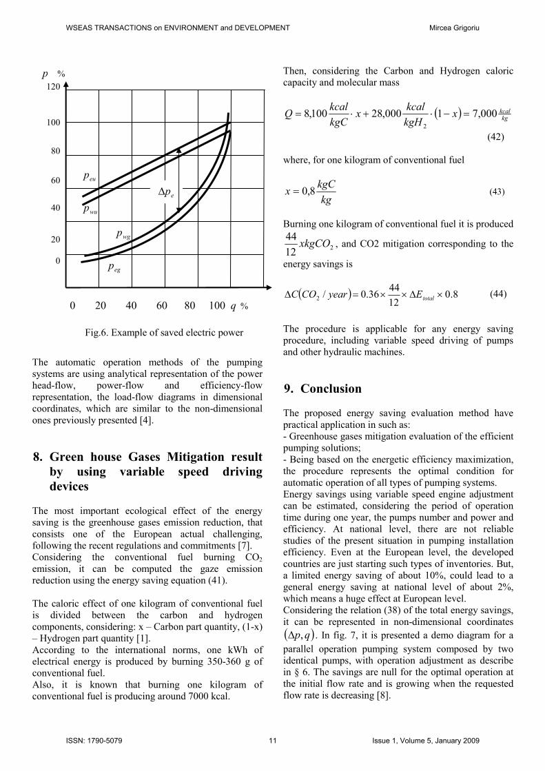
Fig.6. Example of saved electric power
WSEAS TRANSACTIONS on ENVIRONMENT and DEVELOPMENT Mircea Grigoriu
ISSN: 1790-5079 11 Issue 1, Volume 5, January 2009

The most important ecologic effect of the energy
efficiency application is the greenhouse gasses
mitigation, reducing the electrical energy consumption
and, by consequence production [10]. Burning fossil
fuels produces CO2 emissions of roughly 0.53 kg per 1
kWh of electrical energy produced. Thanks to the
drastic reduction in power consumption, the new
system therefore is a positive contribution to
environmental protection.
References:
[1] Grigoriu, M. – Pumps and pumping Installations,
(Romanian language), ISBN 1432-2984, Printing
house Printech, Bucharest, 2006;
[2] Grigoriu, M. – Pumps, Fans, Compressors,
(Romanian language), Printing house Printech,
Bucharest, 1998;
[3] Iliescu, M.; Costoiu, M.; Tonoiu, S. – Study on
Machined Thermal Sprayed Coatings Adherence
(English language), 1st WSEAS International
Conference on SENSORS and SIGNALS (SENSIG
'08), pp 76-81, ISSN 1790-5117, Bucharest, 7-9
November, 2008;
[4] Iliescu, M.; Vlase, A.– New Mathematical Models
of Axial Cutting Force and Torque in Drilling
20MoCr130 Stainless Steel (English language), 10th
WSEAS International Conference on
MATHEMATICAL and COMPUTATIONAL
METHODS in SCIENCE and ENGINEERING
(MACMESE'08), pp 210-215, ISSN 1790-2769,
Bucharest, 7-9 November, 2008;
[5] Grigoriu, M.; Gheorghiu, L. - Energy Efficiency
Pumping Systems Improvement Method. (English
language), Review Energetica, pp 33-38, no.1,
ISSN1453-2360, January 2008;
[6] Grigoriu, M.; Gheorghiu, L.; Hadar, A.; Jiga, G. &
Ciobanu, G. - Pumped-Storage System Operation
Computer Modelling (English language), 0571-0572,
Annals of DAAAM for 2008 & Proceedings of the
19th International DAAAM Symposium, ISBN 978-
3-901509-68-1, ISSN 1726-9679, pp 286-287, Editor
B. Katalinic, Published by DAAAM International,
Vienna, Austria, 23-24 October 2008;
[7] Jiga,G.; Grigoriu,M.; Ciuca,I.; Vlasceanu,D. -
Consideration on Climate Energy Efficiency Impact.
(English language), 0683-0684, Annals of DAAAM
for 2008 & Proceedings of the 19th International
DAAAM Symposium, ISBN 978-3-901509-68-1,
ISSN 1726-9679, pp 342, Editor B. Katalinic,
Published by DAAAM International, Vienna, Austria
23-24 October 2008;
[8] Grigoriu, M.; Gheorghiu, H.; Crai, A.; Dinu, D.;
Visan, D. - Energy Efficiency Evaluation Method.
(English language), 0569-0570, Annals of DAAAM
for 2008 & Proceedings of the 19th International
DAAAM Symposium, ISBN 978-3-901509-68-1,
ISSN 1726-9679, pp 285, Editor B.Katalinic,
Published by DAAAM International, Vienna, Austria
23-24 October 2008;
[9] Grigoriu, M - Energy Saving by Pumped-Storage
system Optimization (English language) – The 8th
International Conference on Technology and Quality
for Sustainable Development (TQSD 2008),
Academy of Technology and Sciences of Romania,
pp 239-244, ISSN 1844-9158, AGIR Publishing
House, 30-31 October 2008;
[10] Grigoriu, m; Gheorghiu, L - Energy Efficiency
Improving Method for Heating Systems (English
language) – Review Energetica, pp 33-38, no.1,
ISSN1453-2360, IJanuary 2008;
[11] * * * - Pump-Control/System Automation, KSB
Know-how, Volume 4, KSB Aktiengesellschaft
Printing, August 2006 Edition.
[12] Noraini A, Zainodin J, Nigel J, Volumetric Stem
Biomass Modeling Using Multiple Regression,
12th WSEAS International Conference on Applied
Mathematics, Cairo, Egypt, December, 2007,
pp 286-291;
[13] Rabia Aktas Altin, A.J.; Nigel, J, .Agenerating
Function and Some Recurrence Relations for a
Family of Polynomials, 12th WSEAS International
Conference on Applied Mathematics, Cairo,
Egypt, December, 2007, pp 118-121.
Electrical power
saving
P∆
80
60
40
20
0
20 40 60 80 100 q %
Fig.7. Explanatory plotting electrical power saving
diagram
WSEAS TRANSACTIONS on ENVIRONMENT and DEVELOPMENT Mircea Grigoriu
ISSN: 1790-5079 12 Issue 1, Volume 5, January 2009
Top Related