


Languages
Pages
Legal


Bank of Canada Banque du Canada
Working Paper 95-8 / Document de travail 95-8
Exchange Rates and Oil Prices
byRobert A. Amano and Simon van Norden


Street,da.ca.
paper
others of theare the
September 1995
Exchange Rates and Oil Prices
Robert A. Amano Simon van NordenResearch Department International Department
Bank of Canada Bank of Canada
Correspondence: Simon van Norden, International Department, Bank of Canada, 234 WellingtonOttawa, Ontario, K1A 0G9, Canada. Fax: (613) 782-7658; e-mail: svannorden@bank-banque-cana
We thank our colleagues at the Bank of Canada for their suggestions. Preliminary versions of thiswere written while Robert Amano was with the International Department of the Bank of Canada.
This paper is intended to make the results of Bank research available in preliminary form toeconomists to encourage discussion and suggestions for revision. The paper represents the viewauthors and does not necessarily reflect those of the Bank of Canada. Any errors or omissionsauthors’.

ISSN 1192-5434
ISBN 0-662-23778-1
Printed in Canada on recycled paper

c price
in why
could
térieur
is. Ils
s des
nt dans
Abstract
The authors document a robust and interesting relationship between the real domesti
of oil and real effective exchange rates for Germany, Japan and the United States. They expla
they think the real oil price captures exogenous terms-of-trade shocks and why such shocks
be the most important factor determining real exchange rates in the long run.
Résumé
Les auteurs mettent en évidence une relation robuste et intéressante entre le prix in
réel du pétrole et les taux de change effectifs réels pour l'Allemagne, le Japon et les États-Un
expliquent pourquoi ils sont d'avis que le prix réel du pétrole saisit les variations exogène
termes de l'échange et pourquoi ces dernières pourraient constituer le facteur le plus importa
la détermination des taux de change réels à long terme.


. . . . . 3
. . . 3
. . . . 5
. . . . 6
. . . . 8
. . . 11
. . . 13
Contents
1. Introduction. . . . . . . . . . . . . . . . . . . . . . . . . . . . . . . . . . . . . . . . . . . . . . . . . . . . . . . . . . . . . 1
2. The Terms of Trade and Exchange Rates . . . . . . . . . . . . . . . . . . . . . . . . . . . . . . . . .
2.1 A Simple Long-Run Model . . . . . . . . . . . . . . . . . . . . . . . . . . . . . . . . . . . . . . . . . .
2.2 Productivity Growth and the Balassa-Samuelson Effect . . . . . . . . . . . . . . . . . . .
2.3 Oil Prices and the Terms of Trade . . . . . . . . . . . . . . . . . . . . . . . . . . . . . . . . . . . .
3. Unit-Root and Cointegration Results . . . . . . . . . . . . . . . . . . . . . . . . . . . . . . . . . . . . .
4. Causality and Exogeneity . . . . . . . . . . . . . . . . . . . . . . . . . . . . . . . . . . . . . . . . . . . . . .
5. Concluding Remarks. . . . . . . . . . . . . . . . . . . . . . . . . . . . . . . . . . . . . . . . . . . . . . . . . .
Tables . . . . . . . . . . . . . . . . . . . . . . . . . . . . . . . . . . . . . . . . . . . . . . . . . . . . . . . . . . . . . . . . . . . . . . 15
Statistical Appendix . . . . . . . . . . . . . . . . . . . . . . . . . . . . . . . . . . . . . . . . . . . . . . . . . . . . . . . . . . . 18
References. . . . . . . . . . . . . . . . . . . . . . . . . . . . . . . . . . . . . . . . . . . . . . . . . . . . . . . . . . . . . . . . . . . 22
Figures. . . . . . . . . . . . . . . . . . . . . . . . . . . . . . . . . . . . . . . . . . . . . . . . . . . . . . . . . . . . . . . . . . . . . . 27


1
odel
(1990),
ls that
e 1980s
ch as
da and
e rates
e ability
sults
4) has
hange
g. The
so it is
other
ee and
(PPP).
f PPP
it is
ture,
t andn thisles
1. Introduction
The exchange rate is arguably the most difficult macroeconomic variable to m
empirically. Surveys of exchange rate models, such as those of Meese (1990) and Mussa
tend to agree on only one point: that existing models are unsatisfactory. Monetary mode
appeared to fit the data for the 1970s are rejected when the sample period is extended to th
(see for example Meese and Rogoff 1983). Later work on the monetary approach, su
Campbell and Clarida (1987), Meese and Rogoff (1988), Edison and Pauls (1993) and Clari
Gali (1994), find that even quite general predictions about the comovements of real exchang
and real interest rates are rejected by the data. In short, there are several reasons to doubt th
of traditional exchange rate models to explain exchange rate movements.
Quite recently, however, we have begun to see more positive (but still controversial) re
emerging in three areas. First, work by researchers such as MacDonald and Taylor (199
shown that a long-run relationship exists among the variables in the monetary model of exc
rates, and that such models perform better than a random walk in out-of-sample forecastin
data, however, reject most of the parameter restrictions imposed by the monetary approach,
uncertain whether these results are really evidence in favor of the monetary model.1 Moreover, this
positive evidence of a long-run monetary model also contrasts with the findings of some
researchers such as Gardeazabal and Regúlez (1992), Sarantis (1994) or Cushman, L
Thorgeirsson (1995).
The second line of research has evolved around the idea of purchasing power parity
As noted by Froot and Rogoff (1994), researchers have found significant evidence in favor o
when they use sufficiently long spans of data. This is a particularly confusing result, since
precisely over such long periods of time that we would expect gradual shifts in industrial struc
relative productivity growth and other factors to alter real equilibrium exchange rates.2
1. Recent Monte Carlo studies (see for example, Toda 1994, Gonzalo and Pitarakis 1994, and Godbouvan Norden 1995) have found that the systems approach to cointegration, an approach often used iliterature, will tend to find evidence of cointegration where none exists in systems with many variab(as is the case with the monetary model of exchange rate determination).
2. For example, see the discussion on Balassa-Samuelson effects in Froot and Rogoff (1994).

2
tions
aining
ns by
ange
anent
Quah
s from
s from
ds and
rsistent
oil
, Japan
prices
, the
the link
1983,
ce for
ls (see
t role
sample
such
ship
hisaxteress.hichure of
Third, structural time-series work on the determinants of real exchange rate fluctua
indicates that real shocks or permanent components play a major and significant role in expl
real exchange rate fluctuations. Univariate and multivariate Beveridge-Nelson decompositio
Huizinga (1987), Baxter (1994) and Clarida and Gali (1994) find that, even though real exch
rates may not follow a random walk, most of their movements are due to changes in the perm
components. Lastrapes (1992) and Evans and Lothian (1993), using the Blanchard and
(1989) decomposition, find that much of the variance of both real and nominal exchange rate
a number of countries over both short and long horizons is due to real shocks. The conclusion
the structural time-series literature therefore seem to be robust to both decomposition metho
currencies. This has led some to suggest that an unidentified real factor may be causing pe
shifts in real equilibrium exchange rates.3
In this paper, we try to identify this real factor by examining the ability of real domestic
prices to account for permanent movements in the real effective exchange rate of Germany
and the United States over the post-Bretton Woods period. The potential importance of oil
for exchange rate movements has been noted by,inter alios, McGuirk (1983), Krugman (1983a,
1983b), Golub (1983) and Rogoff (1991). Although these models are intuitively appealing
empirical work in this area has several important gaps. There have been several studies on
between oil prices and U.S. macroeconomic aggregates (see for example, Hamilton
Loungani 1986, Dotsey and Reid 1992), but exchange rates were not included and eviden
other nations is lacking. There has also been some analysis with calibrated macromode
McGuirk 1983 and Yoshikawa 1990) that suggests that oil price fluctuations play an importan
in exchange rate movements, but these studies lack econometric rigour and consider a data
limited either in length (McGuirk) or number of currencies (Yoshikawa). Some recent papers
as Throop (1993), Zhou (1995) and Dibooglu (1995) find evidence of a long-run relation
3. Many investigating the failure of real interest rate parity relationships have already tried to identify tfactor, without much success (see, for example, Meese and Rogoff 1988, Edison and Pauls 1993, B1994.) Their research has focussed on the explanatory power of fiscal policy and external indebtednOther studies (mentioned below) have used a broader range of explanatory variables. The extent to wother variables cause persistent changes in expected real exchange rates may help to explain the failreal interest rate parity.

3
wever,
ariables
ese
er they
les.
ionale
ction 3
il prices
ults. The
ave an
fficient
n, we
open
f trade.
rate
inally,
data
g a
between exchange rates and a number of macroeconomic factors, including oil prices. Ho
the tests used in these papers tend to produce false evidence of cointegration when several v
are included in the system.4 In addition, they do not examine the causal relationship between th
variables, so it is not clear whether these are models of exchange rate determination or wheth
simply capture the influence of exchange rates on a variety of other macroeconomic variab
The organization of the paper is as follows. The next section describes a possible rat
for the existence of a simple relationship between real exchange rates and oil prices. Se
describes the data used and examines whether or not a stable relationship exists between o
and real exchange rates. Section 4 presents and discusses the exogeneity and causality res
final section offers some concluding remarks.
2. The Terms of Trade and Exchange Rates
As mentioned above, many papers have previously suggested that oil prices may h
important influence on exchange rates. The suggestion, however, that oil prices might be su
to explain all long-run movements in real exchange rates appears to be new. In this sectio
examine the motivation for such a hypothesis. We begin with a simple model of a small
economy in which the exchange rate is determined by exogenous changes in the terms o
Thereafter, we discuss the potential role of productivity differentials in exchange
determination and also consider the evidence linking oil prices to terms-of-trade shocks. F
we briefly comment on the extent to which our results might reasonably be attributed to
mining.
2.1 A Simple Long-Run Model
Consider a small open economy with two sectors, one which produces a traded goodT, and
the other producing a non-traded goodN. Suppose that each sector produces its good usin
constant returns to scale (CRS) technology with a non-traded factorL and a traded factorM as
4. For references, see footnote 1.

4
ectors
trade
of the
be
factor
verage
a
de.
ame
of both
input
ts must
in the
rate.
n the
inputs. Since our analysis will be long-run, we will assume that factors are mobile between s
and that both sectors make zero economic profits.
Let T be the numeraire. This means that , the price ofM, will determine the country’s
terms of trade, with increases in implying an improvement (deterioration) in the terms of
if the country is a net exporter (importer) ofM. We will interpret the price of non-traded goods
as the real exchange rate, with an increase in corresponding to a real appreciation
domestic currency.
The assumption of CRS implies that the cost function for each industry will
homogeneous of degree one in output, so that per-unit production costs will be a function of
prices only. The assumption that economic profits are zero in both sectors then implies that a
production costs will equal output prices. This leads to the pricing equations
(1)
So long asT is produced from bothM and L, we see that the first equation in (1) defines
relationship between and . We can solve this relationship for and (so long asN is
produced from bothM andL) substitute this into the second equation to obtain
(2)
which states that the real value of the exchange rate will be determined by the terms of tra
The intuition behind this result is straightforward. Both sectors compete for the s
inputs. An increase in the price of one of these inputs implies an increase in the average cost
industries. However, costs will rise more in the industry that is the more intensive user of the
whose price has increased. If these industries produce no profits, this change in relative cos
be reflected in equilibrium by a change in the relative price of outputs. However, this change
relative price of traded and non-traded goods in turn implies a change in the real exchange
One might wonder how such an economy would balance its external sector whe
PM
PM
PN
PN
1 T PM PL,( )=
PN N PM PL,( )=
PM PL PL PM( )
PN f PM( )=

5
is that
s is not
ion of
ich in
effect
y the
e
at the
n
hile
both
that
the
they
Most
s have
o their
ect.
exchange rate is independent of demand-side factors. The important point to notice
since both sectors of the economy have a CRS technology, the scale of these sector
determined by the price structure derived above. Instead, given prices, the product
traded and non-traded goods will adjust to clear the market for non-traded goods, wh
turn implies that any budget constraints on external trade will be respected.
2.2 Productivity Growth and the Balassa-Samuelson Effect
Like the model presented in Section 2.1, models of the Balassa-Samuelson
also produce the result that the (long-run) real exchange rate is determined solely b
supply side of the economy.5 These models can differ from the above model in som
important respects, however. First, they typically (although not necessarily) assume th
two factors of production are called capital (M) and labour (L). Second, Balassa-Samuelso
models consider the effects of differential rates of productivity growth across sectors w
sometimes ignoring the effects of factor price changes. A model that allows for
differential rates of sectoral productivity growth and factor price changes would find
these factors will jointly determine the real exchange rate in the long run.
The question of whether relative productivity growth alone can explain
behaviour of real exchange rates has been previously examined.6 Generally speaking,
however, movements in relative productivity are sufficiently small and gradual that
explain little of the overall movements in real exchange rates over the last 20 years.
published studies that focus on relative productivity as a determinant of exchange rate
relied on cross-sectional regressions rather than time-series analysis, but even s
results have been mixed.7
5. See Froot and Rogoff (1994), Section 3.2, for a lucid exposition of the Balassa-Samuelson eff6. See Froot and Rogoff (1994), Sections 3.3 and 3.4.

6
hocks
g this
be
Woods
ause
toral
ts can
at
be
rks.
mall,
n the
ms of
t the
Japan
e use
e do
f oil
Japan
87)mal
nge
One possible reason for these mixed results is the omission of terms-of-trade s
as another factor driving exchange rates. Some cross-sectional evidence supportin
view is presented by De Gregorio and Wolf (1994). In a time-series study, it would
interesting to see the degree to which exchange rate movements in the post-Bretton
period can be jointly explained by relative productivity and terms-of-trade shocks. Bec
of the problems inherent in constructing accurate time series on relative sec
productivity levels, we focus instead on the degree to which exchange rate movemen
be explained by terms-of-trade shocks alone.8 One risk that this approach presents is th
some of the explanatory power of relative productivity shocks might inadvertently
attributed to terms-of-trade shocks. We return to this possibility in our concluding rema
For the time being, we simply note that since relative productivity shocks seem to be s
the omission of relative productivity may not be a serious problem.
2.3 Oil Prices and the Terms of Trade
The model presented in Section 2.1 suggests a unique relationship betwee
terms of trade and the real exchange rate. This will be a causal relationship if the ter
trade are set independently of domestic conditions by world markets. We think tha
latter is unlikely to be the case for industrial economies as large as the United States,
and Germany, however. In the empirical work we present in subsequent sections, w
the real price of oil as a proxy for exogenous changes in the terms of trade. While w
not claim that oil prices would be a useful proxy for all nations, we feel that the price o
is a good approximation for some industrialized nations, such as the United States,
7. Exceptions are the positive results for the yen-dollar exchange rate reported by Marston (19and Yoshikawa (1990), but these relied on calibrated rather than estimated models, so fortests of statistical significance are not available.
8. Amano and van Norden (1995) show that long-run movements in the Canada-U.S. real excharate seem to be caused by movements in components of Canada’s terms of trade.
7
rate
979-80
us a
ves the
that
nd or
d, we
lative to
ve been
real oil
igure 1
in the
gged
.
es in
er than
prices
an that
ade.
terms-
hange
unit
and Germany.
If we examine the behaviour of real oil prices over the most recent floating exchange
period, we see that the series is dominated by major persistent shocks around 1973-74, 1
and 1985-86, with another large but transitory shock in 1990-91. The historical record offers
very plausible explanation for these shocks: they were supply-side shocks that were themsel
result of political conflicts specific to events in the Middle East. Note that we are not arguing
oil prices (or even the stability of price cartels) are immune to the laws of supply and dema
that they cannot be affected by shifts in the growth rates of the industrialized world. Instea
feel that there is ample reason to believe that such demand-side factors have been small re
the supply-side shocks experienced over the last 20 years, and that the supply shocks ha
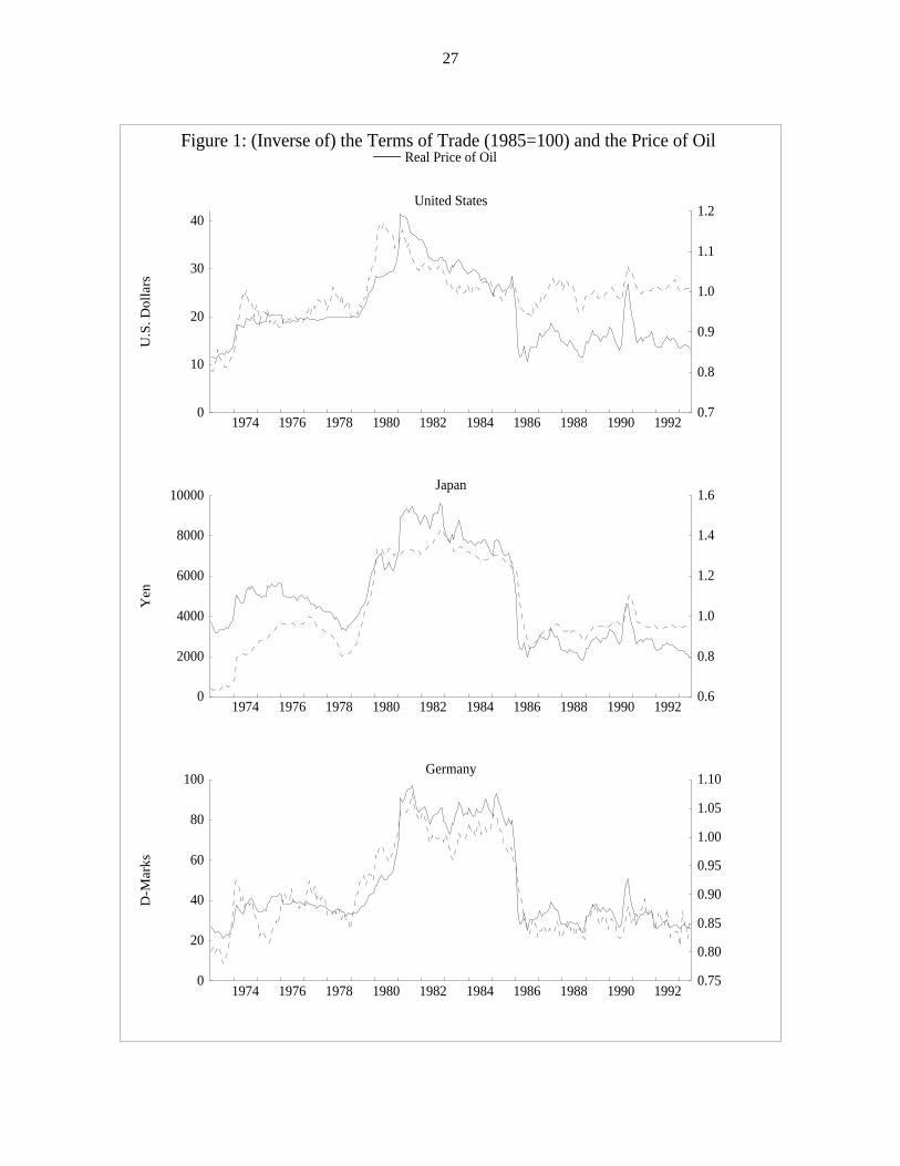
exogenous in the sense of most macroeconomic models. Furthermore, comparing domestic
prices with the terms-of-trade series for each of the United States, Japan and Germany in F
shows that oil prices shocks, indeed, appear to account for most of the major movements
terms of trade.9 In fact, the point correlation between the terms of trade and the one-period-la
price of oil is -0.57, -0.78 and -0.92 for the United States, Japan and Germany, respectively
However, for those skeptical of the use of oil prices as a proxy for exogenous chang
the terms of trade, the appendix presents additional results that use terms-of-trade data rath
real oil prices. These results are broadly similar to the results that we present below using oil
data. Because we feel that the case for exogeneity of the terms of trade is less convincing th
for the real price of oil, we will henceforth consider oil prices rather than the terms of tr
However, we are comforted by the fact that broadly similar results are found using aggregate
of-trade data.
3. Unit-Root and Cointegration Results
In this section, we present evidence of a stable long-run relationship between real exc
9. The terms-of-trade variables are calculated as the ratio between the unit value of exports and thevalue of imports. These data are taken from theInternational Financial Statistics(International MonetaryFund).

8
ective
States
diate
sumer
6.
rom
each
mine
g the
in the
an and
tive
two
series
uires
price
than
rantyt therate.
nee an
the
onsndt ourglts
entful.
rates and real oil prices. The data we use are the Morgan Guaranty 15-country real eff
exchange rate series of Germany (Deutsche mark), Japan (yen) and the United
(dollar), and the domestic price of oil, defined as the U.S. price of West Texas Interme
crude oil converted to the respective currency deflated by the respective country con
price index. The data are observed monthly and cover the period 1973M1 to 1993M10
Figure 2 plots each country’s real exchange rate with its respective real price of oil. F
the figure, it is readily apparent that the real exchange rate and the price of oil for
country are related over the sample period. In the remainder of this section we exa
these relationships in some detail.
Our first step is to examine the time-series properties of each variable usin
augmented Dickey and Fuller (1979) and Phillips and Perron (1988) tests. As shown
appendix, we found that the real effective exchange rates for the United States, Jap
Germany show no strong evidence of long-run PPP.11
Our approach to testing for a long-run relationship between the real effec
exchange rate and the price of oil is to look for evidence of cointegration between the
variables. Assuming that each series has a unit root in its autoregressive time-
representation, a stable long-run equilibrium relationship between the variables req
that they be cointegrated in the sense of Engle and Granger (1987).12 This also allows us to
gauge the adequacy of specifying the real exchange rate simply as a function of the
of oil. If the long-run real exchange rate is determined by nonstationary factors other
10. Although other measures of the real exchange rate are available, we chose the Morgan Gua15-country measure simply because it gave us the longest span of data. We should note tharesults appear robust to different price deflators and measures of the real effective exchangeThe latter is not surprising, as the different measures are very highly correlated (> 0.98).
11. In additional work not reported here, we also found that real interest rate differentials alocannot explain the failure of PPP, and structural decompositions suggest that real shocks arimportant source of persistent real exchange rate movements. These results are available fromauthors.
12. We emphasize that the assumption that the data are I(1) is not crucial to our conclusiconcerning the stability or causality of the relationship we uncover between the price of oil areal exchange rates. For example, one might believe that the data are truly stationary and thafailure to reject the null hypothesis of a unit root is simply due to a lack of power (perhaps owinto an insufficiently long sample.) Under this alternative assumption, the cointegration test resupresented in this section will be of limited interest. However, the evidence which we then preson the measure of this relationship and its apparent Granger causality should still be meaning

9
ficant
that
e real
ingle-
1 yield
hange
ey and
ation
pare
ed by
lius (JJ)
at the
an and
the
ration
o note
e good
in the
roblem
duced
tors—
fully
ators
limiting
the
those associated with the price of oil, then their omission should prevent us from finding signi
evidence of cointegration. Evidence of cointegration, on the other hand, suggests
asymptotically, the price of oil can adequately capture all the permanent innovations in th
effective exchange rate.
We test for cointegration between exchange rates and oil prices using the two-step s
equation approach developed by Engle and Granger (1987). The results presented in Table
strong evidence of cointegration between the price of oil measures and the real effective exc
rates for Germany and Japan but not for the United States. Specifically, the augmented Dick
Fuller (1979) and Phillips and Ouliaris (1990) tests reject the null hypothesis of no cointegr
at the 1 per cent level for the mark, and the 5 and 1 per cent level for the dollar. We then com
these conclusions using an efficient (and therefore more powerful) cointegration test develop
Johansen and Juselius (1990). These results are reported in Table 2. The Johansen-Juse
tests find evidence consistent with cointegration for all three currencies, which suggests th
price of oil captures the permanent innovations in the real exchange rate for Germany, Jap
the United States.
Having found evidence consistent with a long-run relationship, we turn to estimating
long-run response of real effective exchange rates to changes in the price of oil. Cointeg
implies that least-squares (LS) estimates will be super-consistent; however, it is important t
that the rate T-convergence result does not, by itself, ensure that parameter estimates will hav
finite-sample properties. The reason is that LS estimates are not asymptotically efficient,
sense that they have an asymptotic distribution that depends on nuisance parameters. This p
is due to serial correlation in the error term and endogeneity of the regressor matrix that is in
by Granger causation. To control for these problems we use three recently developed estima
Stock and Watson’s (1993) dynamic LS, the prewhitened Phillips and Hansen (1990)
modified LS, and Park’s (1992) canonical cointegrating regression estimators. All three estim
are designed to eliminate nuisance parameter dependencies and possess the same
distribution as full-information-maximum-likelihood estimates, a fact which implies that

10
llows
rison.
es to oil
and
at are
mple,
larger
y 2.4
es be
ates,
Hansen
eter
esults
tests,
also be
e test
study.
lateral
, any
ateral
natory
e of
annot
estimates are asymptotically optimal. The application of the three different estimators also a
us to determine the robustness of the parameter estimates.
Table 3 reports these results along with those from simple LS for the sake of compa
As we can see the LS estimator tends to underestimate the response of real exchange rat
price shocks. Dynamic LS (DLS), prewhitened Phillips and Hansen fully modified LS (FMLS)
Park’s canonical cointegrating regression (CCR) estimators give us long-run estimates th
statistically significant. Regardless of the method used, we find that a rise in oil prices (for exa
of 10 per cent) causes a depreciation of the mark (of roughly 0.9 per cent), an even
depreciation of the yen (of roughly 1.7 per cent), and an appreciation of the dollar (of roughl
per cent).
To interpret these elasticities it is important that the long-run parameters estimat
structurally stable over the sample period. To test for structural stability of the parameter estim
we use a series of parameter constancy tests for I(1) processes recently proposed by
(1992)—theLc, MeanFandSupFtests. All three tests have the same null hypothesis of param
stability but differ in their alternative hypothesis. Specifically, theSupF is useful if we are
interested in testing whether there is a sharp shift in regime, while theLcandMeanFtests are useful
for determining whether or not the specified model captures a stable relationship. The r
presented in Table 4 suggest that we are unable to reject the null hypothesis for any of the
even at the 20 per cent level. We note that Hansen (1992) suggests that these tests may
viewed as tests for the null of cointegration against the alternative of no cointegration. Thus th
results also corroborate our previous conclusion of cointegration among the variables under
Some may argue that because our measure of domestic oil prices uses the bi
exchange rate with the United States to convert U.S. dollar oil prices into a domestic price
evidence of cointegration is simply a result of a common trend between the effective and bil
exchange rates. We investigated this possibility by using the bilateral rate as the expla
variable in the place of the real domestic price of oil. With this change, we find no evidenc
cointegration, even at the 10 per cent significance level. Moreover, such an explanation c

11
. real
ctive
point
tem
results
ts the
hile
e note
ange
ely,
ry and
n and
while
en oil
affect
ector
atson
s of one
time.
er-
explain the evidence of cointegration found between real U.S. dollar oil prices and the U.S
exchange rate. Finally, if we are simply capturing a relationship between bilateral and effe
exchange rates, we should not find unidirectional causality in our systems. We address this
in the next section.
4. Causality and Exogeneity
From Engle and Granger (1987) we know that cointegration in a two-variable sys
implies that at least one of the variables must Granger-cause the other. However the
presented above do not indicate whether the long-run relationship we have found reflec
endogeneity of the domestic price of oil or the determination of the exchange rate, or both. W
understanding the causal links between these variables may be interesting in its own right, w
that if causality runs from the price of oil to the exchange rate, this would also imply that exch
rate changes are forecastable, and therefore that semi-strong market efficiency is rejected.
Our first step in testing for causality is to test for “long-run causality,” or more accurat
to test whether any of our variables are weakly exogenous in the sense of Engle, Hend
Richard (1983). This can be tested using the likelihood-ratio test described in Johanse
Juselius (1990). The results shown in Table 5 imply that the price of oil is weakly exogenous,
the real exchanges are not. This implies that deviations from the long-run relationship betwe
prices and exchanges significantly influence exchange rates, but do not significantly
domestic oil prices.
Next we test for more general Granger causality using standard tests on the v
autoregression level representation of our system. As demonstrated in Sims, Stock and W
(1990), standard inference procedures are valid in this case under the maintained hypothesi
cointegrating vector, provided that we test the exclusion restrictions on one variable at a
These results are reported in Table 6.13 They indicate strong evidence that the price of oil Grang
causes the real exchange rate, whereas there is no evidence of the reverse.

12
es as
arent
er is
tted)
, but
cific
likely
mple
in the
likely
ould
ice
es is
ior to
gate
index,
their
y of
t the
even
ical
ag-heesehe
If we accept the conclusion that exchange rates do not Granger-cause oil pric
our empirical evidence suggests, what other interpretation can we offer for the app
long-run relationship between these two variables? An important possibility to consid
that oil prices and exchange rates are jointly determined by some third (omi
macroeconomic variable. This would imply that we have a reduced-form relationship
not one that should be thought of as a structural or causal link. Without a spe
alternative, this is not a criticism that we can test. Nonetheless, we feel that this is un
to be the case. As we argued in Section 2.3, the behaviour of oil prices over our sa
period is dominated by major persistent supply shocks that have been exogenous
sense of most macroeconomic models. Accordingly, few macroeconomic insights are
to be gained from a search for a co-determinant of exchange rates and oil prices.
Previous formal analysis of this question in the case of the United States w
seem to support our view. In particular, Hamilton’s (1983) claim that major oil pr
increases preceded almost all post–World War II recessions in the United Stat
accompanied by an extensive search for a variable that was Granger-causally-pr
domestic U.S. oil prices. After exploring a wide range of variables, including aggre
prices, wages, real output, monetary aggregates, bond yields and a stock-price
Hamilton finds that almost none seemed to cause oil prices and none could explain
effect on output.14 As for the monetary and fiscal variables that have been the mainsta
modern exchange rate modelling, we have already cited studies which show tha
explanatory power of these variables for exchange rates is limited. Furthermore,
13. Since all results are based on asymptotic approximations we use the limiting chi-square critvalues instead of their more common F-distributed counterparts.
14. Apparently causal-prior variables were import prices (weak evidence that is sensitive to the llength used), coal prices and the ratio of person-days idle due to strike to total employment. Tfirst two could simply reflect the same external energy supply shocks, but might response to thshocks more quickly than domestic energy prices. The latter variable may simply reflect tinfluence of strikes by U.S. coal miners on domestic energy prices in the 1950s.
13
ed by
unt of
Reid
with
ishes
ices
-run
ween
nd the
nous
actor
r the
ships
think
ore
res of
o be
ials in
ates
hich
tes.
nted.
supposedly exogenous measures of monetary policy such as that recently propos
Romer and Romer (1989) for the United States may capture a considerable amo
endogenous policy reaction to exogenous external oil prices. Indeed, Dotsey and
(1992) show that Romer and Romer’s measure of monetary policy is coincident
several major oil price shocks and that its explanatory power for output variables van
when oil prices are included in the system. We therefore think it is unlikely that oil pr
are simply acting as a proxy for some other macroeconomic determinant of long
exchange rates.
5. Concluding Remarks
We have documented what we think is a robust and interesting relationship bet
the real domestic price of oil and real effective exchange rates for Germany, Japan a
United States. We have also explained why we think the real oil price captures exoge
terms-of-trade shocks, and why such shocks could be the most important f
determining real exchange rates in the long run. Given the ongoing debate ove
determination of exchange rates and the other work we have cited examining relation
between exchange rates and the terms of trade for other industrialized countries, we
that this is an area that deserves further research.
This research could be usefully extended in several directions. Obviously, m
evidence could be gathered, perhaps for additional currencies, for additional measu
the terms of trade, or from additional testing methods. As we noted earlier, it would als
reasonable to see whether our results are robust to the inclusion of sectoral different
productivity growth, although we have suggested that this is likely to be the case.
More structural work on the relationship between oil prices and exchange r
would also be useful. The terms-of-trade model we presented is only one of many w
predict that oil prices will have important effects on industrial-country exchange ra
More detailed testing and comparison of these competing models may be warra

14
factor
Finally, attempts to relate the size of the long-run elasticities reported in Table 3 to sectoralintensities would also be of interest.

15
d
Table 1:Augmented Dickey-Fuller (ADF) and Phillips-Ouliaris (PO) Tests for Cointegrationa
a. ADF and PO critical values are taken from MacKinnon (1994). The lag length for the ADFtest is selected on the basis of a data-dependent method suggested by Ng and Perron (1994)using a 5 per cent critical value. The initial number of ADF lags is set equal to the seasonalfrequency plus 1 or 13. The PO test statistic is calculated using the prewhitened QS kernelestimator with the automatic bandwidth parameter advocated by Andrews and Monahan (1992).For Tables 1 and 2, ** and * indicate significance at the 1 and 5 per cent levels.
Regression Lags AEG t-statistic PO -statistic
mark 9 -3.98** -41.75**
yen 8 -3.82* -34.79**
dollar 12 -2.19 -11.204
Table 2:Johansen and Juselius Tests for Cointegrationa
a. We performed the tests under the assumption that the cointegrating vector annihilates any driftterms in the exchange rate or price of oil. Tests of this restriction are available from the authors.Thecritical values are taken from Johansen and Juselius (1990). Lag lengths are determined using standarlikelihood ratio tests. We begin with 13 lags and use a 5 per cent critical value. r denotes the number ofcointegrating vectors.
Trace Statistic Max. Statistic
Equation Lags
mark 5 19.81* 3.84 15.98* 3.84
yen 4 20.60* 2.61 17.99* 2.61
dollar 4 21.89* 4.76 15.123* 4.76
Zα
Zα
λ
r 1≤ r 0≤ r 1≤ r 0≤

16
Table 3: Estimation of the Static Equationa
The Estimated Effect of Oil Prices on Exchange Rates
a. Standard errors are in parentheses. The FMLS estimates are based on the VAR(2)prewhitening procedure of Andrews and Monahan (1992), as this gave us seriallyuncorrelated residuals. The DLS estimates are based on sixth-order leads and lags andNewey and West (1987) standard errors calculated using a truncation parameter equal to theseasonal frequency or 12. The CCR estimates are from the third stage of estimation assuggested by Park and Ogaki (1991).
EstimationMethod
mark yen dollar
LS -0.079 -0.156 0.141
FMLS -0.086 (0.011) -0.170 (0.029) 0.276 (0.089)
DLS -0.083 (0.010) -0.158 (0.022) 0.174 (0.059)
CCR -0.092 (0.014) -0.201 (0.047) 0.258 (0.058)
Table 4:Hansen Stability Tests of the Cointegrating Vectora
a. We use the FMLS estimates from Table 3 to calculate these test statistics. The reportedvalues in parentheses are p-values.
Equation Lc MeanF SupF
mark 0.380 (> 0.09) 2.493 (> 0.20) 4.447 (> 0.20)
yen 0.111 (> 0.20) 1.334 (> 0.20) 3.087 (> 0.20)
dollar 0.260 (> 0.19) 2.421 (> 0.20) 5.451 (> 0.20)

17
Table 5:Johansen Weak Exogeneity Testsa
a. Reported numbers are p-values (the lowest significance level at which we can reject thenull hypothesis).
Equation Lags: Price of oil is
weakly exogenous: Exchange rate is
weakly exogenous
mark 5 0.414 < 0.000
yen 4 0.158 < 0.000
dollar 4 0.901 0.001
Table 6:Granger-Causality Testsa
a. Reported numbers are p-values (the lowest significance level at which we can reject thenull hypothesis).
Equation Lags: Price of oil does not
cause exchange rates: Exchange rates do
not cause oil prices
mark 5 0.002 0.239
yen 4 0.012 0.422
dollar 4 0.017 0.857
H0 H0
H0 H0

18
Table
ption
d 5 per
hoose
ective
try real
nations’
from
Q3 to
Statistical Appendix
Unit-Root Tests
Unit-root test results for the real exchange rate and real oil price series are reported in
A1. We are unable to reject the null hypothesis of a unit root for any of the series, with the exce
of the German exchange rate. For the latter, the test statistics are between the 1 per cent an
cent critical values. Since we feel that there may be some doubt about this conclusion, we c
to include this series in our cointegration analysis nonetheless.
Tests Using Terms-of-Trade Data
At an earlier stage of our research, we examined the relationship between the real eff
exchange rate and the terms of trade. The data we used were the Morgan Guaranty 40-coun
effective exchange rate series for the United States, Germany and Japan, and the same
terms of trade, defined as the ratio of export to import unit values in U.S. dollars and taken
the IMF data base (lines 74d and 75d). The data are quarterly and cover the period 1973
Table A1: Augmented Dickey-Fuller (ADF) and Phillips-Perron (PP) Tests“*” indicates significance at the 5 per cent level
Nation Series ADF a
a. All test regressions include a constant term. The lag selection procedureis that suggested by Ng and Perron (1994). The number of lags used isshown in parentheses.
PP b
b. The long-run variance is estimated using an AR(1) prewhitenedquadratic spectral kernel estimator and a data-dependent bandwidthparameter, as suggested by Andrews and Monahan (1992).
U.S. Exchange Rate -1.68 (1) -5.82
Oil Price -2.22 (2) -12.87
Germany Exchange Rate -3.06* (9) -14.00*
Oil Price -1.88 (2) -8.85
Japan Exchange Rate -2.51 (4) -10.73
Oil Price -1.22 (7) -5.50
τ Zα
19
e I(1),
-run
refore,
n.
shown
rating
nce of
econd
long-
an and
e null
for the
sistent
y
1992Q1.15
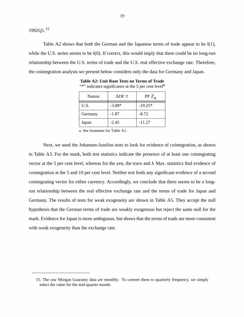
Table A2 shows that both the German and the Japanese terms of trade appear to b
while the U.S. series seems to be I(0). If correct, this would imply that there could be no long
relationship between the U.S. terms of trade and the U.S. real effective exchange rate. The
the cointegration analysis we present below considers only the data for Germany and Japa
Next, we used the Johansen-Juselius tests to look for evidence of cointegration, as
in Table A3. For the mark, both test statistics indicate the presence of at least one cointeg
vector at the 5 per cent level, whereas for the yen, the trace and Max. statistics find evide
cointegration at the 5 and 10 per cent level. Neither test finds any significant evidence of a s
cointegrating vector for either currency. Accordingly, we conclude that there seems to be a
run relationship between the real effective exchange rate and the terms of trade for Jap
Germany. The results of tests for weak exogeneity are shown in Table A5. They accept th
hypothesis that the German terms of trade are weakly exogenous but reject the same null
mark. Evidence for Japan is more ambiguous, but shows that the terms of trade are more con
with weak exogeneity than the exchange rate.
15. The raw Morgan Guaranty data are monthly. To convert them to quarterly frequency, we simplselect the value for the mid-quarter month.
Table A2: Unit Root Tests on Terms of Trade“*” indicates significance at the 5 per cent levela
a. See footnotes for Table A1.
Nation ADF PP
U.S. -3.88* -19.25*
Germany -1.87 -8.72
Japan -2.45 -11.27
τ Zα
λ

20
vector
nce of
nited
use the
at more
ars to
es that
there
erse.
Table A5 shows the results of tests for Granger causality using standard tests on the
autoregression level representation of the systems. Since this does not require evide
cointegration, results for the United States are included once more. The evidence for the U
States and for Germany allow us to conclude that the terms of trade appear to Granger-ca
real exchange rate, whereas the reverse is not true. The conclusions for Japan are somewh
difficult to interpret. If we use the 5 per cent significance levels, then neither variable appe
Granger-cause the other. However, we should recall that the presence of cointegration impli
Granger causality should exist in at least one direction. With this in mind, we simply note that
is more evidence of the terms of trade Granger-causing the real exchange rate than the rev
Table A3: Johansen-Juselius (JJ) Test for CointegrationEstimation under Assumption of Restricted Drift
“*” indicates significance at the 5 per cent level
Trace Statistic Max. Statistic JJ Lagsa
a. Appropriate lag lengths are determined using standard likelihood ratio tests with a finite-sample correction.
Mark 20.925* 16.536* 2
4.389 4.389
Yen 21.484* 14.871 2
6.613 6.613
Table A4: Weak Exogeneity Tests
NationVariable under the Null of Weak
ExogeneitySignificance Level
Germany Terms of Trade 0.682
Exchange Rate 0.001
Japan Terms of Trade 0.102
Exchange Rate 0.066
λ
r 1≤
r 0≤
r 1≤
r 0≤

21
e real
is of a
h the
om the
three
In summary, we found evidence of cointegration between the German and Japanes
effective exchange rates and their corresponding terms of trade. We rejected the hypothes
unit root in the U.S. terms of trade, which therefore implies the absence of cointegration wit
U.S. real effective exchange rate. The results also show no evidence of Granger-causality fr
exchange rate to the terms of trade but significant evidence of the reverse for two of the
nations.
Table A5: Granger Causality Results
DependentVariable
IndependentVariable
Number ofLagsa
a. Lag lengths were selected on the basis of the Akaike information criteria.
SignificanceLevel
U.S. ExchangeRate
U.S. Terms ofTrade
1 0.020
U.S. Terms ofTrade
U.S. ExchangeRate
3 0.857
GermanExchange Rate
German Terms ofTrade
1 0.003
German Terms ofTrade
GermanExchange Rate
2 0.719
JapaneseExchange Rate
Japanese Termsof Trade
2 0.129
Japanese Termsof Trade
JapaneseExchange Rate
4 0.301
22
s: the
and
ment
and
HowA.
hoodCD
Real
arity.”
ive
ic
hange
tion:
anent
References
Amano, Robert and Simon van Norden. 1995. “Terms of trade and real exchange rateCanadian evidence.”Journal of International Money and Finance, 14(1):83-104.
Andrews, Donald W. K. and J. Christopher Monahan. 1992. “An Improved HeteroskedasticityAutocorrelation Consistent Covariance Matrix Estimator.”Econometrica 60: 953-66.
Baxter, Marianne 1994. “Real Exchange Rates, Real Interest Differentials, and GovernPolicy: Theory and Evidence.”Journal of Monetary Economics 33: 5-37.
Blanchard, Olivier J. and Danny Quah. 1989. “The Dynamic Effect of Aggregate DemandSupply Disturbance.”American Economic Review 79: 655-73.
Campbell, John Y. and Richard H. Clarida. 1987. “The dollar and real interest rates.”Carnegie-Rochester Conference Series on Public Policy 27: 103-40.
Clarida, Richard H. and Jordi Gali. 1994. “Sources of Real Exchange Rate Fluctuations:Important are Nominal Shocks?” Working Paper No. 4658. NBER, Cambridge, MForthcoming inCarnegie-Rochester Conference Series on Public Policy.
Cushman, David O., Sang S. Lee and Thorsteinn Thorgeirsson. 1995. “Maximum LikeliEstimates of Cointegration in Exchange Rate Models for Seven Inflationary OECountries.” Forthcoming inJournal of International Money and Finance.
De Gregorio, José and Holger C. Wolf. 1994. “Terms of Trade, Productivity, and theExchange Rate.” Working Paper 4807. NBER, Cambridge, MA.
Dibooglu, Selahattin. 1995. “Real Disturbances, Relative Prices, and Purchasing Power PForthcoming inSouthern Journal of Economics.
Dickey, David A. and Wayne A. Fuller. 1979. “Distribution of the Estimator for AutoregressTime Series with a Unit Root.”Journal of the American Statistical Association74:427-31.
Dotsey, M. and M. Reid. 1992. “Oil Shocks, Monetary Policy and Economic Activity.” EconomReview. Federal Reserve Bank of Richmond, Richmond, VA. 14-27.
Edison, Hali J. and B. D. Pauls. 1993. “A re-assessment of the relationship between real excrates and the real interest rates: 1974-1990.”Journal of Monetary Economics 31: 165-87.
Engle, Robert F., and Clive W. J. Granger. 1987. “Cointegration and Error CorrecRepresentation, Estimation and Testing.”Econometrica 55:251-76.
Engle, R. F., D. F. Hendry and J. F. Richard. 1983. “Exogeneity.”Econometrica 51:277-304.
Evans, Martin D. D. and James R. Lothian. 1993. “The response of exchange rates to permand transitory shocks under floating exchange rates.”Journal of International Money andFinance12:563-586.
23
hange
nd
hangeat the
imeo.
sses.”
tes”
ood
ge
o
tes.”
ong-
and
Froot, Kenneth A. and Kenneth Rogoff. 1994. “Perspectives on PPP and Long-Run Real ExcRates.” NBER Working Paper No. 4952. Forthcoming inThe Handbook of InternationalEconomics.
Gardeazabal, Javier and Marta Regúlez. 1992.The monetary model of exchange rates acointegration: estimation, testing and prediction.Springer-Verlag.
Godbout, Marie-Josée and Simon van Norden. 1995. “Reconsidering cointegration in excrates: Case studies of size distortion in finite samples.” manuscript for presentation1996 Winter Meetings of the Econometric Society.
Golub, Stephen S. 1983. “Oil Prices and Exchange Rates.”Economic Journal 93: 576-93.
Gonzalo, Jesus and J.-Y. Pitarakis. 1994. “Cointegration Analysis in Large Systems.” mBoston University, Boston, MA.
Hamilton, James D. 1983. “Oil and the Macroeconomy since World War II.”Journal of PoliticalEconomy 91: 228-48.
Hansen, Bruce E. 1992. “Tests for Parameter Instability in Regressions with I(1) ProceJournal of Business & Economic Statistics 10:321-35.
Huizinga, J. 1987. “An empirical investigation of the long-run behavior of real exchange raCarnegie-Rochester Series on Public Policy, 27, 149-215.
Johansen, Soren and Katarina Juselius. 1990. “The full information maximum likelihprocedure for inference on cointegration.”Oxford Bulletin of Economics and Statistics52:169-210.
Krugman, Paul. 1983a. “Oil and the dollar.” InEconomic Interdependence and Flexible ExchanRates, edited by J. S. Bhandari and B. H. Putnam. Cambridge: MIT Press.
Krugman, Paul. 1983b. “Oil shocks and exchange rate dynamics.” InExchange Rates andInternational Macroeconomics, edited by J. A. Frankel. Chicago: University of ChicagPress.
Lastrapes, William D. 1992. “Sources of Fluctuations in Real and Nominal Exchange RaReview of Economics and Statistics74: 530-39.
Loungani, P. 1986. “Oil Price Shocks and the Dispersion Hypothesis.”Review of Economics andStatistics 68: 536-39.
MacDonald, Ronald and Mark P. Taylor. 1994. “The Monetary Model of the Exchange Rate: LRun Relationships, Short-Run Dynamics and How to Beat a Random Walk,” Journal ofInternational Money and Finance13: 276-90.
MacKinnon, James G. 1994. “Approximate Asymptotic Distribution Functions for Unit-RootCointegration Tests.”Journal of Business & Economic Statistics12: 167-76.

24
s and
strial
nties:
ential
nce,tion,
ite,
dent
eningfor
ables
ts for
ions.”
ange, CA.
n theic
Marston, Richard. 1987. “Real Exchange Rates and Productivity Growth in the United StateJapan.” InReal-Financial Linkages among Open Economies, edited by S. Arndt and J. D.Richardson. Cambridge: MIT Press.
McGuirk, Anne K. 1983. “Oil price changes and real exchange rate movements among inducountries,”International Monetary Fund Staff Papers 30: 843-83.
Meese, Richard A. 1990. “Currency Fluctuations in the Post-Bretton Woods Era.”Journal ofEconomic Perspectives 4: 117-34.
Meese, Richard A. and Kenneth Rogoff. 1983. “Empirical exchange rate models of the SeveDo they fit out of sample?”Journal of International Economics 14: 3-24.
Meese, Richard A. and Kenneth Rogoff. 1988. “Was it real? The exchange rate-interest differrelation over the modern floating-rate period.”The Journal of Finance 43: 933-48.
Mussa, M. L. 1990. “Exchange Rates in Theory and in Reality.” Essays in International FinaNo. 179, Princeton University, Department of Economics, International Finance SecPrinceton, NJ.
Newey, Whitney K. and Kenneth D. West. 1987. “A Simple, Positive Semi-DefinHeteroskedasticity and Autocorrelation Consistent Covariance Matrix.”Econometrica55:703-8.
Ng, Serena and Pierre Perron. 1994. “Unit root tests in ARMA models with data depenmethods for the selection of the truncation lag.” Forthcoming inJournal of the AmericanStatistical Association.
Park, Joon Y. 1992. “Canonical Cointegrating Regressions.”Econometrica 60: 119-43.
Park, Joon Y. and Masao Ogaki. 1991. “Inference in Cointegrated Models using VAR Prewhitto Estimate Short-Run Dynamics.” Working Paper No. 281. Rochester CenterEconomic Research, University of Rochester, Rochester.
Phillips, Peter C. B. and Bruce E. Hansen. 1990. “Statistical Inference in Instrumental VariRegression with I(1) Processes.”Review of Economic Studies 57:99-125.
Phillips, Peter C. B. and Sam Ouliaris. 1990. “Asymptotic Properties of Residual Based TesCointegration.”Econometrica 58:165-93.
Phillips, Peter C. B. and Pierre Perron. 1988. “Testing for a Unit Root in Time Series RegressBiometrika75: 335-46.
Rogoff, Kenneth. 1991. “Oil, productivity, government spending and the real yen-dollar exchrate.” Working Paper 91-06. Federal Reserve Bank of San Francisco, San Francisco
Romer, Christine D. and David H. Romer. 1989. “Does monetary policy matter? A new test ispirit of Friedman and Schwartz.”National Bureau of Economic Research MacroeconomAnnual4: 122-70.
25
irical
eries
rs in
tes.”
ear
Sarantis, Nicholas. 1994. “The monetary exchange rate model in the long run: an empinvestigation.”Weltwirtschaftliches Archiv, p. 698-711.
Sims, Christopher A., James H. Stock and Mark W. Watson. 1990. “Inference in linear time smodels with some unit roots.”Econometrica 58: 113-44.
Stock, James H. and Mark W. Watson. 1993. “A Simple Estimator of Cointegrating VectoHigher Order Integrated Systems.”Econometrica60: 783-820.
Throop, Adrian W. 1993. “A generalized uncovered interest parity model of exchange raEconomic Review, Federal Reserve Bank of San Francisco, 2, 3-16.
Toda, Hiro Y. 1994. “Finite sample properties of likelihood ratio tests for cointegration when lintrends are present.”Review of Economics and Statistics76: 66-79.
Yoshikawa, Hiroshi. 1990. “On the Equilibrium Yen-Dollar Rate.”American Economic Review,80: 576-83.
Zhou, Su. 1995. “The Response of Real Exchange Rates to Various Economic Shocks.”SouthernEconomic Journal XX: 936-54.

26
27
Figure 1: (Inverse of) the Terms of Trade (1985=100) and the Price of OilReal Price of Oil
1974 1976 1978 1980 1982 1984 1986 1988 1990 19920
10
20
30
40
0.7
0.8
0.9
1.0
1.1
1.2United States
U.S
. D
olla
rs
1974 1976 1978 1980 1982 1984 1986 1988 1990 19920
2000
4000
6000
8000
10000
0.6
0.8
1.0
1.2
1.4
1.6Japan
Ye
n
1974 1976 1978 1980 1982 1984 1986 1988 1990 19920
20
40
60
80
100
0.75
0.80
0.85
0.90
0.95
1.00
1.05
1.10Germany
D-M
ark
s

28
Figure 2: Effective Exchange Rates and the Price of Oil
1974 1976 1978 1980 1982 1984 1986 1988 1990 19920
10
20
30
40
80
100
120
140
Real U.S. Price of OilReal U.S. Effective Exchange Rate
U.S
. D
olla
rs
1974 1976 1978 1980 1982 1984 1986 1988 1990 19920
2000
4000
6000
8000
10000
70
80
90
100
110
120
130
Real Japanese Price of Oil(Inverse of) Real Japanese Effective Exchange Rate
Ye
n
1974 1976 1978 1980 1982 1984 1986 1988 1990 19920
20
40
60
80
100
90
95
100
105
110
Real German Price of Oil(Inverse of) Real German Effective Exchange Rate
D-M
ark
s

Bank of Canada Working Papers
1995
95-1 Deriving Agents’ Inflation Forecasts from the Term Structureof Interest Rates C. Ragan
95-2 Estimating and Projecting Potential Output Using Structural VAR A. DeSerres, A. GuayMethodology: The Case of the Mexican Economy and P. St-Amant
95-3 Empirical Evidence on the Cost of Adjustment and Dynamic Labour Demand R. A. Amano
95-4 Government Debt and Deficits in Canada: A Macro Simulation Analysis T. Macklem, D. Roseand R. Tetlow
95-5 Changes in the Inflation Process in Canada: Evidence and Implications D. Hostland
95-6 Inflation, Learning and Monetary Policy Regimes in the G-7 Economies N. Ricketts and D. Rose
95-7 Analytical Derivatives for Markov-Switching Models J. Gable, S. van Nordenand R. Vigfusson
95-8 Exchange Rates and Oil Prices R. A. Amano and S. van Norden
1994(Earlier 1994 papers, not listed here, are also available.)
94-6 The Dynamic Behaviour of Canadian Imports and the Linear- R. A. AmanoQuadratic Model: Evidence Based on the Euler Equation and T. S. Wirjanto
94-7 L’endettement du secteur privé au Canada : un examen macroéconomique J.-F. Fillion
94-8 An Empirical Investigation into Government Spending R. A. Amanoand Private Sector Behaviour and T. S. Wirjanto
94-9 Symétrie des chocs touchant les régions canadiennes A. DeSerreset choix d’un régime de change and R. Lalonde
94-10 Les provinces canadiennes et la convergence : une évaluation empirique M. Lefebvre
94-11 The Causes of Unemployment in Canada: A Review of the Evidence S. S. Poloz
94-12 Searching for the Liquidity Effect in Canada B. Fung and R. Gupta
Single copies of Bank of Canada papers may be obtained from Publications DistributionBank of Canada234 Wellington StreetOttawa, Ontario K1A 0G9
E-mail: [email protected]
The papers are also available by anonymous FTP to thefollowing address, in the subdirectory /pub/publications: ftp.bank-banque-canada.ca
Top Related