


Languages
Pages
Legal

Field Report
Avian Community Composition and Blood Mercury and Chromium in
Onondaga Lake Wastebeds
Submitted to
Anne Secord U.S. Fish and Wildlife Service
New York Field Office (Region 5) 3817 Luker Road
Cortland, NY 13045
Submitted by Jonathan Cohen and Anand Chaudhary Dept. Environmental and Forest Biology
SUNY College of Environmental Science and Forestry 1 Forestry Drive
Syracuse, NY 13210
Submitted: January 2014

i
TableofContentsPage No.
Background ................................................................................................................................................... 1
Justification ................................................................................................................................................... 1
Field effort summary .................................................................................................................................... 1
Study area ..................................................................................................................................................... 2
Point counts .................................................................................................................................................. 2
Mist netting and blood sample collection ..................................................................................................... 3
Invertebrate sample collection ...................................................................................................................... 3
Vegetation sampling ..................................................................................................................................... 3
Winter nest study .......................................................................................................................................... 4
Laboratory analysis for mercury and chromium ........................................................................................... 4
Data analysis ................................................................................................................................................. 5
Results for mercury and chromium analysis ................................................................................................. 5
References ..................................................................................................................................................... 6

1
Avian Community Composition and Blood Mercury and Chromium in Onondaga Lake Wastebeds
Background Onondaga Lake is one of the important lakes in the Finger Lakes region of Central New York which drains into Lake Ontario. Located close to the City of Syracuse, it is important for recreational use. This lake is sacred to the Onondaga Nation and is considered a “birth place of democracy” because warring nations came together here to form the Haudenosaunee confederacy (Onondaga Lake Partnership 2010).
Onondaga Lake is a Federal Superfund site listed by EPA in 1994 (Onondaga Lake Partnership 2010) due to industrial and municipal discharge of hazardous material into the lake for over 100 years. The lake is contaminated with PCBs, PAHs, VOCs, and heavy metals like mercury, chromium, lead, and cobalt. As much as 9 kilograms (kg) of mercury per day was released by industry into the lake at one point (Onondaga Lake Partnership 2010). Disposal of soda ash waste along the lake shore has led to the creation of huge mounds simply known now as the “wastebeds.” The wastebeds rise 15 meters (m) from the lake shore and cover over one square kilometer (km2). Waste from the production of soda ash was pumped to settling basins adjacent to the lake shore since Solvay Process Company started producing soda ash in 1884 (Onondaga Lake Partnership 2010). The water evaporated, leaving a chalky white alkaline substrate. The Allied Chemical plant disposed its waste on these beds for nearly 30 years until 1943. The wastebeds were acquired by New York State in 1953 and portions of it subsequently by Onondaga County (Michalenko 1991). The wastebeds have become vegetated through natural succession and from 2004 - 2008 through restoration with plant communities dominated by willow scrub/shrub, aspen (Populus deltoides) forest, and grassland. An initial study of wildlife communities in the wastebeds indicated the presence of shrubland and grassland birds, including song sparrow (Melospiza melodia), red-winged blackbird (Agelaius phoeniceus), American robin (Turdus migratorius), and warblers (Campbell et al. 2012).
Justification Mercury and chromium are among the most hazardous pollutants documented at the lake. Mercury has been found to cause hatching and fledging failures in birds; chromium is known to affect their growth and behavior (Burger and Gochfeld 2000; Evers et al. 2012). This study will ascertain if birds on the wastebeds are being exposed to these metals. We will also study abundance and diversity of birds to provide information on the value of the area to native avifauna. The results would provide information on potential contaminant exposure risks to birds and will help aid understanding on the implications for waste bed management and habitat restoration projects.
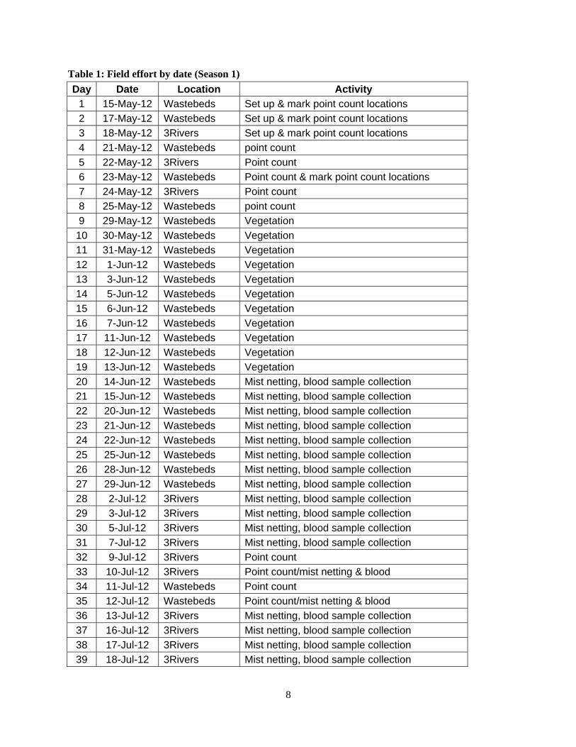
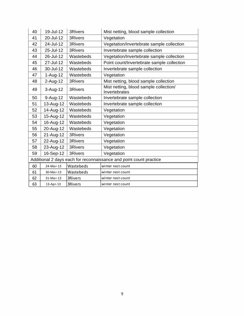
Field effort summary Season 1 (2012): A total of 67 days (140 person-days) were spent in field work during the summer at the research and reference sites (Table 1). This included two days each for reconnaissance surveys and practice for points and five days with support from volunteers. A field technician started field work from 15 May 2012 and left her position at the end of first week of August. A second field technician was hired
2
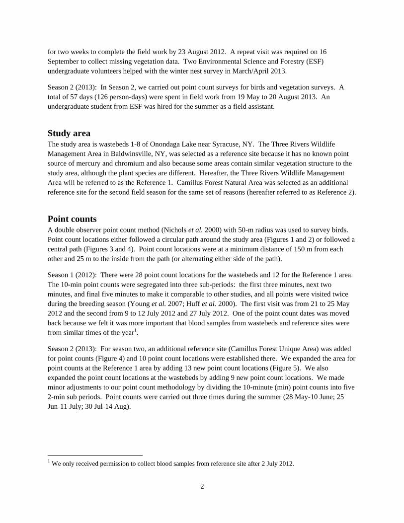
for two weeks to complete the field work by 23 August 2012. A repeat visit was required on 16 September to collect missing vegetation data. Two Environmental Science and Forestry (ESF) undergraduate volunteers helped with the winter nest survey in March/April 2013.
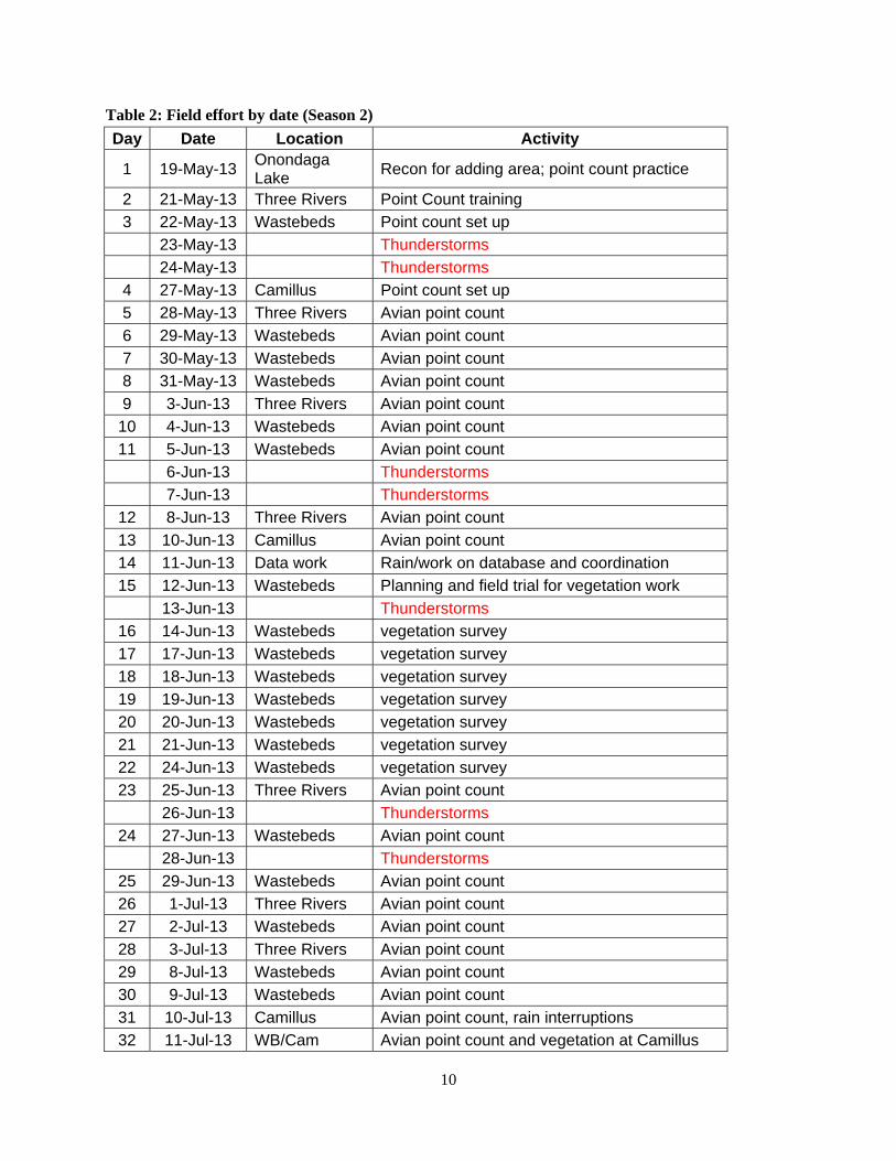
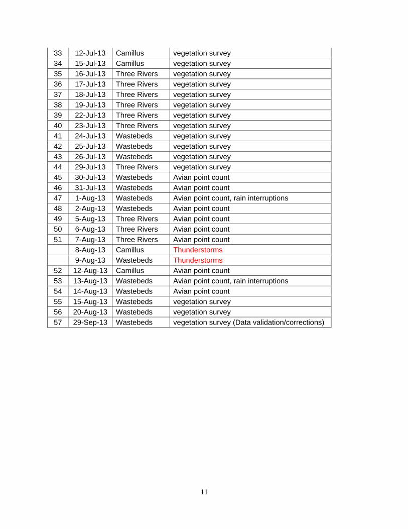
Season 2 (2013): In Season 2, we carried out point count surveys for birds and vegetation surveys. A total of 57 days (126 person-days) were spent in field work from 19 May to 20 August 2013. An undergraduate student from ESF was hired for the summer as a field assistant.
Study area The study area is wastebeds 1-8 of Onondaga Lake near Syracuse, NY. The Three Rivers Wildlife Management Area in Baldwinsville, NY, was selected as a reference site because it has no known point source of mercury and chromium and also because some areas contain similar vegetation structure to the study area, although the plant species are different. Hereafter, the Three Rivers Wildlife Management Area will be referred to as the Reference 1. Camillus Forest Natural Area was selected as an additional reference site for the second field season for the same set of reasons (hereafter referred to as Reference 2).
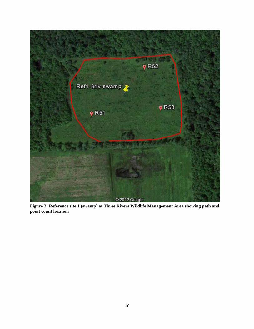
Point counts A double observer point count method (Nichols et al. 2000) with 50-m radius was used to survey birds. Point count locations either followed a circular path around the study area (Figures 1 and 2) or followed a central path (Figures 3 and 4). Point count locations were at a minimum distance of 150 m from each other and 25 m to the inside from the path (or alternating either side of the path).
Season 1 (2012): There were 28 point count locations for the wastebeds and 12 for the Reference 1 area. The 10-min point counts were segregated into three sub-periods: the first three minutes, next two minutes, and final five minutes to make it comparable to other studies, and all points were visited twice during the breeding season (Young et al. 2007; Huff et al. 2000). The first visit was from 21 to 25 May 2012 and the second from 9 to 12 July 2012 and 27 July 2012. One of the point count dates was moved back because we felt it was more important that blood samples from wastebeds and reference sites were from similar times of the year1.
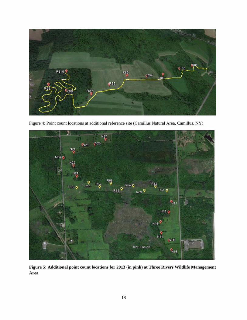
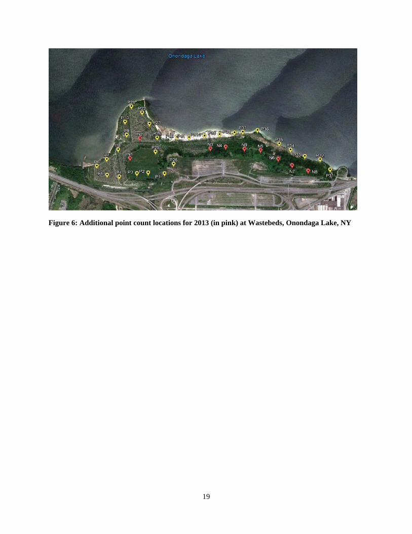
Season 2 (2013): For season two, an additional reference site (Camillus Forest Unique Area) was added for point counts (Figure 4) and 10 point count locations were established there. We expanded the area for point counts at the Reference 1 area by adding 13 new point count locations (Figure 5). We also expanded the point count locations at the wastebeds by adding 9 new point count locations. We made minor adjustments to our point count methodology by dividing the 10-minute (min) point counts into five 2-min sub periods. Point counts were carried out three times during the summer (28 May-10 June; 25 Jun-11 July; 30 Jul-14 Aug).
1 We only received permission to collect blood samples from reference site after 2 July 2012.
3
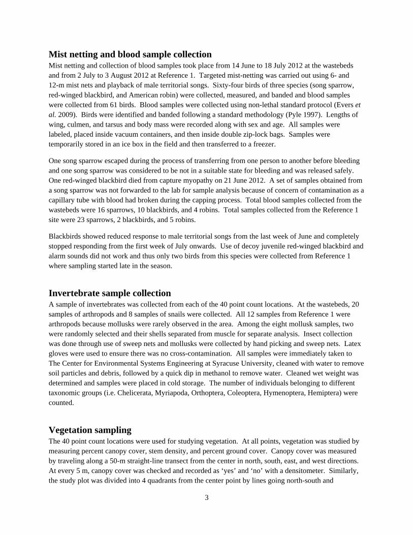
Mist netting and blood sample collection Mist netting and collection of blood samples took place from 14 June to 18 July 2012 at the wastebeds and from 2 July to 3 August 2012 at Reference 1. Targeted mist-netting was carried out using 6- and 12-m mist nets and playback of male territorial songs. Sixty-four birds of three species (song sparrow, red-winged blackbird, and American robin) were collected, measured, and banded and blood samples were collected from 61 birds. Blood samples were collected using non-lethal standard protocol (Evers et al. 2009). Birds were identified and banded following a standard methodology (Pyle 1997). Lengths of wing, culmen, and tarsus and body mass were recorded along with sex and age. All samples were labeled, placed inside vacuum containers, and then inside double zip-lock bags. Samples were temporarily stored in an ice box in the field and then transferred to a freezer.
One song sparrow escaped during the process of transferring from one person to another before bleeding and one song sparrow was considered to be not in a suitable state for bleeding and was released safely. One red-winged blackbird died from capture myopathy on 21 June 2012. A set of samples obtained from a song sparrow was not forwarded to the lab for sample analysis because of concern of contamination as a capillary tube with blood had broken during the capping process. Total blood samples collected from the wastebeds were 16 sparrows, 10 blackbirds, and 4 robins. Total samples collected from the Reference 1 site were 23 sparrows, 2 blackbirds, and 5 robins.
Blackbirds showed reduced response to male territorial songs from the last week of June and completely stopped responding from the first week of July onwards. Use of decoy juvenile red-winged blackbird and alarm sounds did not work and thus only two birds from this species were collected from Reference 1 where sampling started late in the season.
Invertebrate sample collection A sample of invertebrates was collected from each of the 40 point count locations. At the wastebeds, 20 samples of arthropods and 8 samples of snails were collected. All 12 samples from Reference 1 were arthropods because mollusks were rarely observed in the area. Among the eight mollusk samples, two were randomly selected and their shells separated from muscle for separate analysis. Insect collection was done through use of sweep nets and mollusks were collected by hand picking and sweep nets. Latex gloves were used to ensure there was no cross-contamination. All samples were immediately taken to The Center for Environmental Systems Engineering at Syracuse University, cleaned with water to remove soil particles and debris, followed by a quick dip in methanol to remove water. Cleaned wet weight was determined and samples were placed in cold storage. The number of individuals belonging to different taxonomic groups (i.e. Chelicerata, Myriapoda, Orthoptera, Coleoptera, Hymenoptera, Hemiptera) were counted.
Vegetation sampling The 40 point count locations were used for studying vegetation. At all points, vegetation was studied by measuring percent canopy cover, stem density, and percent ground cover. Canopy cover was measured by traveling along a 50-m straight-line transect from the center in north, south, east, and west directions. At every 5 m, canopy cover was checked and recorded as ‘yes’ and ‘no’ with a densitometer. Similarly, the study plot was divided into 4 quadrants from the center point by lines going north-south and
4
east-west. A point-quarter technique was used to estimate stem density. The nearest shrub, small tree (diameter <3cm), and large tree were measured for diameter at breast height (dbh) and height. A grid with 64 cells (10 cm x 10 cm) was used to estimate percent ground cover. The grid was placed at the center and at 25 m and 50 m in all four compass directions and any items (grass, herbaceous plant, soil, leaf litter, moss, etc.) that fell below the cross-hairs were recorded (49 cross-hairs).
In the 2013 summer season, canopy cover and grid analysis were carried out for vegetation in all 72 point count locations. In addition, we also identified dominant plants at each grid location to the species level where possible.
Winter nest study Nests were searched within 50m radius of the 40 established point count locations. Two people searched randomly for 10 minutes within the area and marked any nests spotted. After the 10-minute survey, nests were photographed, GPS locations were recorded, and data on inner and outer diameter and height from ground level were measured for those nests that were easily reachable. In some areas where study sites had been disturbed by construction, less than 10 minutes were required to cover the entire area. A total of 78 nests were found from the 12 point count locations at the reference site. At Onondaga Lake, 45 nests were found; however, many of the 28 point count locations had been destroyed (completely or partially) by road construction and expansion activity.
Laboratory analysis for mercury and chromium The samples were submitted to The Center for Environmental Systems Engineering at Syracuse University on 28 August 2012. Results for blood mercury were received from the lab on 2 October 2012 (Table 3) and for invertebrate mercury on 8 December 2012 (Table 4). Results for blood chromium were made available in July 2013 (Table 5). Final results of chromium in invertebrates after a rerun of samples for outliers was made available in December 2013 (Table 4).
Mercury (Hg): The terrestrial samples were freeze dried for 72 hours (Labconco, Kansas City, MO), and then the samples were homogenized into a fine powder for total Hg (THg). Blood samples were collected in capillary tubes, and the total volume collected was weighed and analyzed for total mercury. THg analyses were performed on a Mercury Analyzer (DMA-80 Direct, Milestone, Shelton, CT; or LECO AMA, LECO Corp., St. Joseph, MI) utilizing thermal decomposition, catalytic reduction, amalgamation, desorption, and atomic absorption spectroscopy. The method detection limit (MDL) for solids is 0.1 ng/g. Instruments were calibrated with DORM-2 and DORM-3 Standard Reference Materials. Reference Material 2976 (mussel tissue) was used as quality control reference material, and all results were within plus and minus 10% recoveries of the 61 certified concentrations.
Chromium: The blood samples and freeze dried and homogenized samples were transferred to a glass vial and digested with 2 ml of nitric acid and 2 ml of hydrogen peroxide in an oven at 65 degrees Celsius for 24 hours. Samples were diluted to a 10 ml final volume. Additional dilutions were performed as required. QCS sample was digested with the samples. The digested sample was nebulized into a spray chamber where a stream of argon carried the sample aerosol through a quartz torch and injected it into an argon plasma stream. There the sample was vaporized and component atoms were ionized. The ions
5
produced were entrained in the plasma gas and introduced into a high-vacuum that housed a quadruple mass spectrometer. The ions were sorted according to their mass-to-charge ratio and measured with a detector. For the daily operation, the ELAN® 6000 ICP-MS was tuned and optimized. The instrument was externally calibrated; continuing calibration verification and calibration blanks were run every 10 samples and a second certified source standard was run to verify the calibration curve.
Data analysis Data analysis was carried out using SAS software. We have used medians in reporting the results when we have had to log transform the variables for analysis. When a variable is log transformed, its mean is the same as its median and when back transformed the median is now the median (and not the mean) of the original variable.
Results for mercury and chromium analysis Avian blood mercury results: Median avian blood mercury levels were compared in blood samples between the wastebeds and reference sites. Mercury levels were found to be significantly higher at the wastebeds for song sparrows (ANOVA F5,54=9.44, P<0.001 wet weight [ww]), but not for other species (Figure 7). Blood mercury concentrations varied from 1.93 ppm ww in a red-winged blackbird from the wastebeds to no detection in an American robin also from the wastebeds.
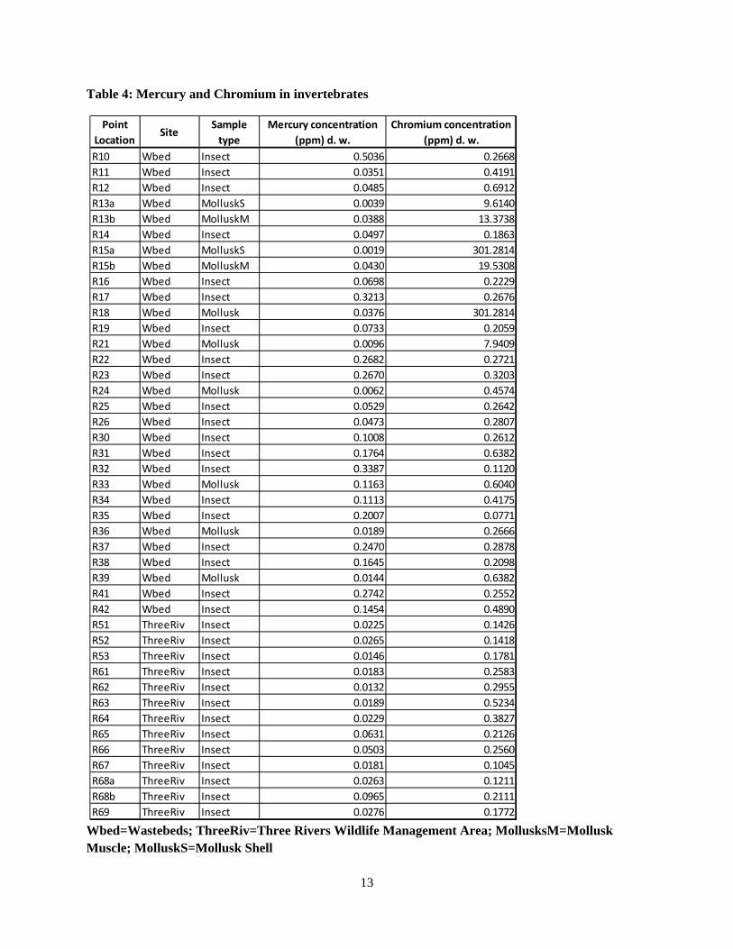
Invertebrate mercury results: Analysis of arthropods (insects, arachnids, and isopods) median mercury levels revealed significantly higher mercury in arthropods of the wastebeds (ANOVA, preplanned contrast F1=26.93, P<0.0001 dry weight [dw]) (Figure 8). To better understand the data, samples from the wastebeds were further divided into those samples collected from the shore of Onondaga Lake along the northeastern part of the study area with those collected from western part of the study area (Figure 9) at the two different locations (Powerline and Swamp) of Reference 1. The samples from along the lake shore were found to have higher mercury concentration (ANOVA, F3, 29=23.84, P<0.0001 dw) (Figure 10) and there was a significant difference between the two areas of the wastebeds (ANOVA, preplanned contrast F1=13.24, P<0.0009 dw).
Mollusk samples from the wastebeds were compared among each other to see if concentrations varied between shell and muscle (Figure 11). Muscle contained significantly higher concentrations of mercury than the shell (ANOVA, preplanned contrast F1=12.52, P<0.0011 dw). Samples with no separation of muscle and shell also contained significantly high concentrations of mercury compared to samples with shell only (ANOVA, preplanned contrast F1=10.34, P<0.0027 dw), but the difference was not significant in comparison to samples with muscle only (ANOVA, preplanned contrast F1=1.26, P<0.2691 dw).
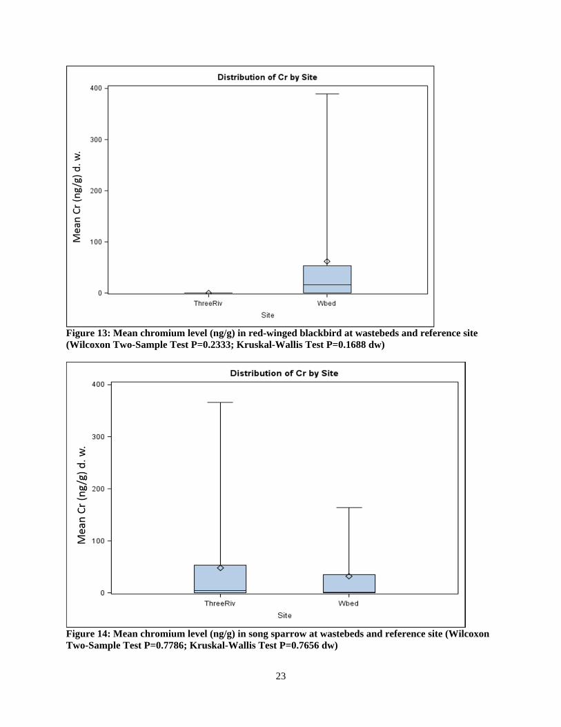
Mean avian blood chromium results were not significantly different between the wastebeds and Reference 1 for American robin (Wilcoxon Two-Sample Test P=0.3382; Kruskal-Wallis Test P=0.2444 dw) (Figure 12); red-winged blackbird (Wilcoxon Two-Sample Test P=0.2333; Kruskal-Wallis Test P=0.1688 dw) (Figure 13); and song sparrow (Wilcoxon Two-Sample Test P=0.7786; Kruskal-Wallis Test P=0.7656 dw) (Figure 14).
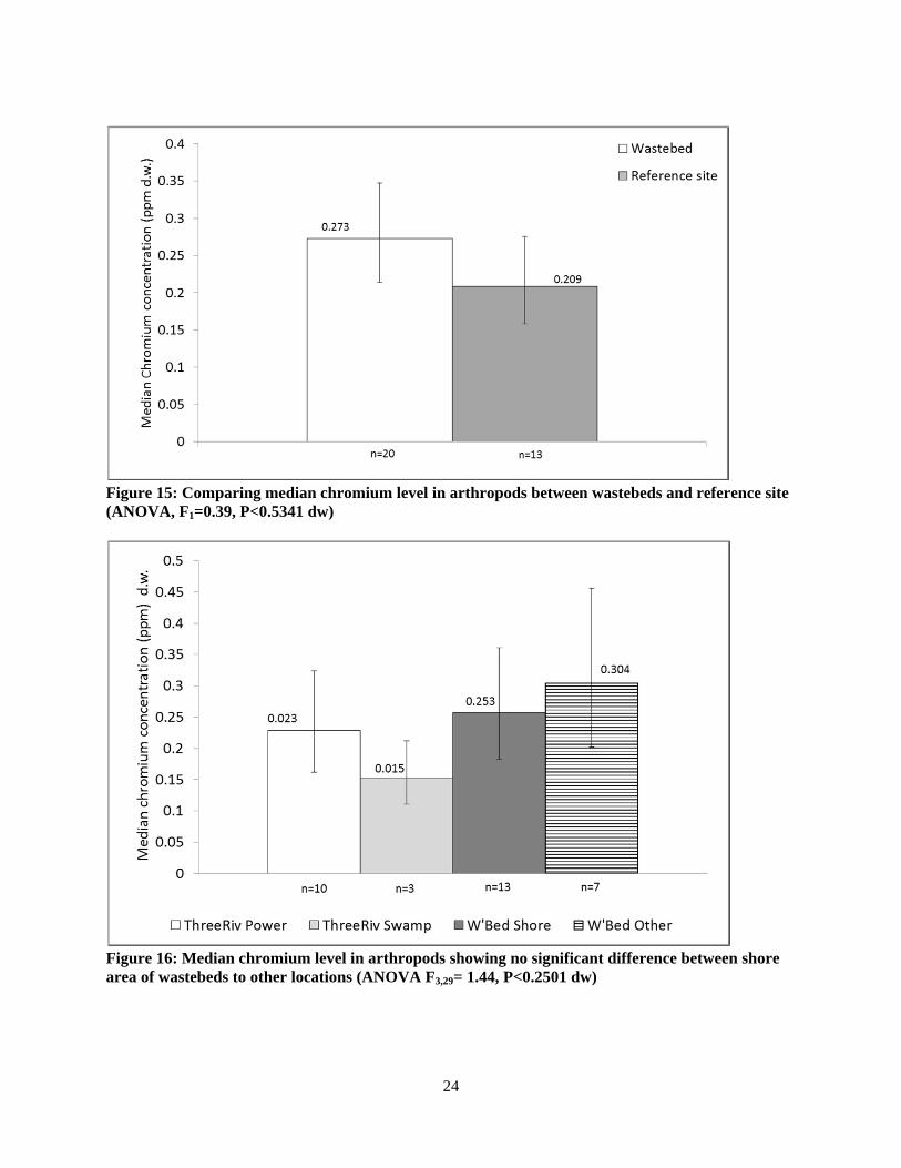
Invertebrate chromium results: Analysis of arthropods (insects, arachnids, and isopods) median chromium levels revealed no significant difference in chromium in arthropods of the wastebeds and

6
Reference 1 (ANOVA, F1=0.39, P<0.5341 dw) (Figure 15). Like in the case of mercury, we compared the samples from the shore of Onondaga Lake along the northeastern part of the study area with those collected from the western part of the study area (Figure 9) to the two different locations (Powerline and Swamp) of the reference site. The samples from along the lake shore were found to not have any significant difference in chromium concentration (ANOVA F3,29= 1.44, P<0.2501 dw) (Figure 16) and there was no significant difference between the two areas of the wastebeds (ANOVA, preplanned contrast F1=0.1, P<0.7596 dw).
Mollusk samples from the wastebeds were compared among each other to see if concentrations varied between shell and muscle. Shell contained significantly higher concentrations of chromium than the samples without separation of shell and muscle (ANOVA, preplanned contrast F1=11.76, P<0.0015 dw). There were no significant differences between samples with no separation of muscle and shell compared to samples with muscle only (ANOVA, preplanned contrast F1=4.58, P<0.0389 dw) and between shell and muscle samples (ANOVA, preplanned contrast F1=1.11, P<0.2989 dw) (Figure 17).
Preliminary results were presented in a poster at The Wildlife Society Annual Meeting in Portland, OR, on 15 October 2012 and in Milwaukee, WI, on 7 October 2013. Additional results were presented at Northeast Fish and Wildlife Conference at Saratoga Springs, NY, 7-9 April 2013. Analysis of species richness, abundance, and vegetation is ongoing and will be reported as a part of Anand Chaudhary’s master’s thesis.
References Campbell, S.P., J.L. Frair, J.P. Gibbs, and T.A. Volk. (2012). Use of short rotation coppice willow crops
by birds and small mammals in central New York. Biomass and Energy 45: 342-353. Burger, J. and M. Gochfeld. 2000. Growth and behavioral effects of early postnatal chromium exposure
in herring gull (Larus argentatus) chicks. Pharmacology, Biochemistry and Behavior 50:607-612. Evers, D.C., K.A. Williams, and M. Duron. 2009. Protocol for TERRA Network: Sampling songbirds,
bats, invertebrates, litterfall and soil for contaminant analysis. Report BRI 2009-17, Biodiversity Research Institute, Gorham, Maine.
Evers, D.C., A.K. Jackson, T.H. Tear, and C.E. Osborne. 2012. Hidden risk: Mercury in terrestrial
ecosystems of the northeast. Gorham, Maine: Biodiversity Research Institute. Report nr BRI Report 2012-07.
Huff, M.H., K.A. Bettinger, H.L. Ferguson, M.J. Brown, and B. Altman. 2000. A habitat based point
count protocol for terrestrial birds, emphasizing Washington and Oregon. United States Forest Service general technical report PNW-GTR-501. Portland, Oregon, USA.
Michalenko, E.M. 1991. Pedogenesis and invertebrate microcommunity succession in immature soils
originating from chlor-alkali wastes. Doctoral thesis. SUNY College of Environmental Science and Forestry, Syracuse, New York, USA.
Nichols, J.D., J.E. Hines, J.T. Sauer, F.W. Fallon, J.E. Fallon, and P.J. Heglund. 2000. Double-observer
approach for estimating detection probability and abundance from point counts. The Auk 117: 393-408.
7
Onondaga Lake Partnership. 2010. The State of Onondaga Lake 2010. Onondaga Lake Partnership,
Syracuse, NY. Pyle, P. 1997. Identification Guide to North American Birds. Part 1. Slate Creek Press, Bolinas,
California, USA. Young, J.S., A. Cilimburg, K. Smucker, and R.L. Hutto. 2007. Point Count Protocol-2007. Northern
region land bird monitoring program. Avian Science Center. <avianscience.dbs.umt.edu/research_landbird_methodsmanual> Accessed 10 May 2012
8
Table 1: Field effort by date (Season 1)
Day Date Location Activity
1 15-May-12 Wastebeds Set up & mark point count locations
2 17-May-12 Wastebeds Set up & mark point count locations
3 18-May-12 3Rivers Set up & mark point count locations
4 21-May-12 Wastebeds point count
5 22-May-12 3Rivers Point count
6 23-May-12 Wastebeds Point count & mark point count locations
7 24-May-12 3Rivers Point count
8 25-May-12 Wastebeds point count
9 29-May-12 Wastebeds Vegetation
10 30-May-12 Wastebeds Vegetation
11 31-May-12 Wastebeds Vegetation
12 1-Jun-12 Wastebeds Vegetation
13 3-Jun-12 Wastebeds Vegetation
14 5-Jun-12 Wastebeds Vegetation
15 6-Jun-12 Wastebeds Vegetation
16 7-Jun-12 Wastebeds Vegetation
17 11-Jun-12 Wastebeds Vegetation
18 12-Jun-12 Wastebeds Vegetation
19 13-Jun-12 Wastebeds Vegetation
20 14-Jun-12 Wastebeds Mist netting, blood sample collection
21 15-Jun-12 Wastebeds Mist netting, blood sample collection
22 20-Jun-12 Wastebeds Mist netting, blood sample collection
23 21-Jun-12 Wastebeds Mist netting, blood sample collection
24 22-Jun-12 Wastebeds Mist netting, blood sample collection
25 25-Jun-12 Wastebeds Mist netting, blood sample collection
26 28-Jun-12 Wastebeds Mist netting, blood sample collection
27 29-Jun-12 Wastebeds Mist netting, blood sample collection
28 2-Jul-12 3Rivers Mist netting, blood sample collection
29 3-Jul-12 3Rivers Mist netting, blood sample collection
30 5-Jul-12 3Rivers Mist netting, blood sample collection
31 7-Jul-12 3Rivers Mist netting, blood sample collection
32 9-Jul-12 3Rivers Point count
33 10-Jul-12 3Rivers Point count/mist netting & blood
34 11-Jul-12 Wastebeds Point count
35 12-Jul-12 Wastebeds Point count/mist netting & blood
36 13-Jul-12 3Rivers Mist netting, blood sample collection
37 16-Jul-12 3Rivers Mist netting, blood sample collection
38 17-Jul-12 3Rivers Mist netting, blood sample collection
39 18-Jul-12 3Rivers Mist netting, blood sample collection
9
40 19-Jul-12 3Rivers Mist netting, blood sample collection
41 20-Jul-12 3Rivers Vegetation
42 24-Jul-12 3Rivers Vegetation/Invertebrate sample collection
43 25-Jul-12 3Rivers Invertebrate sample collection
44 26-Jul-12 Wastebeds Vegetation/Invertebrate sample collection
45 27-Jul-12 Wastebeds Point count/Invertebrate sample collection
46 30-Jul-12 Wastebeds Invertebrate sample collection
47 1-Aug-12 Wastebeds Vegetation
48 2-Aug-12 3Rivers Mist netting, blood sample collection
49 3-Aug-12 3Rivers Mist netting, blood sample collection/ Invertebrates
50 9-Aug-12 Wastebeds Invertebrate sample collection
51 13-Aug-12 Wastebeds Invertebrate sample collection
52 14-Aug-12 Wastebeds Vegetation
53 15-Aug-12 Wastebeds Vegetation
54 16-Aug-12 Wastebeds Vegetation
55 20-Aug-12 Wastebeds Vegetation
56 21-Aug-12 3Rivers Vegetation
57 22-Aug-12 3Rivers Vegetation
58 23-Aug-12 3Rivers Vegetation
59 16-Sep-12 3Rivers Vegetation
Additional 2 days each for reconnaissance and point count practice
60 24‐Mar‐13 Wastebeds winter nest count
61 30‐Mar‐13 Wastebeds winter nest count
62 31‐Mar‐13 3Rivers winter nest count
63 13‐Apr‐13 3Rivers winter nest count
10
Table 2: Field effort by date (Season 2)
Day Date Location Activity
1 19-May-13 Onondaga Lake
Recon for adding area; point count practice
2 21-May-13 Three Rivers Point Count training
3 22-May-13 Wastebeds Point count set up
23-May-13 Thunderstorms
24-May-13 Thunderstorms
4 27-May-13 Camillus Point count set up
5 28-May-13 Three Rivers Avian point count
6 29-May-13 Wastebeds Avian point count
7 30-May-13 Wastebeds Avian point count
8 31-May-13 Wastebeds Avian point count
9 3-Jun-13 Three Rivers Avian point count
10 4-Jun-13 Wastebeds Avian point count
11 5-Jun-13 Wastebeds Avian point count
6-Jun-13 Thunderstorms
7-Jun-13 Thunderstorms
12 8-Jun-13 Three Rivers Avian point count
13 10-Jun-13 Camillus Avian point count
14 11-Jun-13 Data work Rain/work on database and coordination
15 12-Jun-13 Wastebeds Planning and field trial for vegetation work
13-Jun-13 Thunderstorms
16 14-Jun-13 Wastebeds vegetation survey
17 17-Jun-13 Wastebeds vegetation survey
18 18-Jun-13 Wastebeds vegetation survey
19 19-Jun-13 Wastebeds vegetation survey
20 20-Jun-13 Wastebeds vegetation survey
21 21-Jun-13 Wastebeds vegetation survey
22 24-Jun-13 Wastebeds vegetation survey
23 25-Jun-13 Three Rivers Avian point count
26-Jun-13 Thunderstorms
24 27-Jun-13 Wastebeds Avian point count
28-Jun-13 Thunderstorms
25 29-Jun-13 Wastebeds Avian point count
26 1-Jul-13 Three Rivers Avian point count
27 2-Jul-13 Wastebeds Avian point count
28 3-Jul-13 Three Rivers Avian point count
29 8-Jul-13 Wastebeds Avian point count
30 9-Jul-13 Wastebeds Avian point count
31 10-Jul-13 Camillus Avian point count, rain interruptions
32 11-Jul-13 WB/Cam Avian point count and vegetation at Camillus
11
33 12-Jul-13 Camillus vegetation survey
34 15-Jul-13 Camillus vegetation survey
35 16-Jul-13 Three Rivers vegetation survey
36 17-Jul-13 Three Rivers vegetation survey
37 18-Jul-13 Three Rivers vegetation survey
38 19-Jul-13 Three Rivers vegetation survey
39 22-Jul-13 Three Rivers vegetation survey
40 23-Jul-13 Three Rivers vegetation survey
41 24-Jul-13 Wastebeds vegetation survey
42 25-Jul-13 Wastebeds vegetation survey
43 26-Jul-13 Wastebeds vegetation survey
44 29-Jul-13 Three Rivers vegetation survey
45 30-Jul-13 Wastebeds Avian point count
46 31-Jul-13 Wastebeds Avian point count
47 1-Aug-13 Wastebeds Avian point count, rain interruptions
48 2-Aug-13 Wastebeds Avian point count
49 5-Aug-13 Three Rivers Avian point count
50 6-Aug-13 Three Rivers Avian point count
51 7-Aug-13 Three Rivers Avian point count
8-Aug-13 Camillus Thunderstorms
9-Aug-13 Wastebeds Thunderstorms
52 12-Aug-13 Camillus Avian point count
53 13-Aug-13 Wastebeds Avian point count, rain interruptions
54 14-Aug-13 Wastebeds Avian point count
55 15-Aug-13 Wastebeds vegetation survey
56 20-Aug-13 Wastebeds vegetation survey
57 29-Sep-13 Wastebeds vegetation survey (Data validation/corrections)

12
Table 3: Blood Mercury in birds
SOSP=Song Sparrow, AMRO=American Robin, RWBL=Red-Winged Blackbird; ND = No detection at detection limit 0.1ng/g
Sample Species Location Hg (ppm) w.w. Sample Specie Location Hg (ppm) w.w.
1222‐37‐905 AMRO Wastebeds 0.3356 2581‐11‐408 SOSP Wastebeds 0.7496
1222‐37‐909 AMRO Wastebeds ND 2581‐11‐424 SOSP Wastebeds 0.4393
1222‐37‐910 AMRO Wastebeds 0.2371 2581‐11‐425 SOSP Wastebeds 0.3394
1222‐37‐911 AMRO Wastebeds 0.0829 2581‐11‐426 SOSP Wastebeds 0.3267
1222‐37‐916 AMRO Three Rivers 0.0386 2581‐11‐432 SOSP Wastebeds 0.0741
1222‐37‐917 AMRO Three Rivers 0.0244 2581‐11‐433 SOSP Wastebeds 0.1217
1222‐37‐918 AMRO Three Rivers 0.0189 2581‐11‐434 SOSP Wastebeds 0.3657
1222‐37‐919 AMRO Three Rivers 0.0315 2581‐11‐429 SOSP Three Rivers 0.0323
1222‐37‐920 AMRO Three Rivers 0.0213 2581‐11‐409 SOSP Three Rivers 0.0627
1222‐37‐901 RWBL Wastebeds 1.9348 2581‐11‐410 SOSP Three Rivers 0.0494
1222‐37‐902 RWBL Wastebeds 0.6635 2581‐11‐411 SOSP Three Rivers 0.0414
1222‐37‐903 RWBL Wastebeds 0.1581 2581‐11‐412 SOSP Three Rivers 0.1068
1222‐37‐904 RWBL Wastebeds 1.1446 2581‐11‐413 SOSP Three Rivers 0.0495
1222‐37‐906 RWBL Wastebeds 0.2426 2581‐11‐415 SOSP Three Rivers 0.0608
1222‐37‐908 RWBL Wastebeds 0.1238 2581‐11‐418 SOSP Three Rivers 0.0443
1222‐37‐912 RWBL Wastebeds 0.2473 2581‐11‐419 SOSP Three Rivers 0.0685
1222‐37‐913 RWBL Wastebeds 0.2151 2581‐11‐420 SOSP Three Rivers 0.0865
1222‐37‐914 RWBL Wastebeds 0.1385 2581‐11‐421 SOSP Three Rivers 0.1094
2561‐75‐503 RWBL Wastebeds 0.2751 2581‐11‐422 SOSP Three Rivers 0.0499
1222‐37‐915 RWBL Three Rivers 0.4017 2581‐11‐423 SOSP Three Rivers 0.0901
2581‐11‐414 RWBL Three Rivers 0.3095 2581‐11‐427 SOSP Three Rivers 0.0695
2581‐11‐405 SOSP Wastebeds 0.1715 2581‐11‐430 SOSP Three Rivers 0.0861
2561‐75‐501 SOSP Wastebeds 0.7249 2581‐11‐431 SOSP Three Rivers 0.1188
2561‐75‐502 SOSP Wastebeds 0.4689 2581‐11‐435 SOSP Three Rivers 0.0380
2581‐11‐401 SOSP Wastebeds 0.4903 2581‐11‐436 SOSP Three Rivers 0.0616
2581‐11‐402 SOSP Wastebeds 0.7409 2581‐11‐437 SOSP Three Rivers 0.0415
2581‐11‐403 SOSP Wastebeds 0.6826 2581‐11‐438 SOSP Three Rivers 0.0787
2581‐11‐404 SOSP Wastebeds 0.4950 2581‐11‐439 SOSP Three Rivers 0.0196
2581‐11‐406 SOSP Wastebeds 0.2709 2581‐11‐440 SOSP Three Rivers 0.0304
2581‐11‐407 SOSP Wastebeds 0.9806 2581‐11‐441 SOSP Three Rivers 0.0773
13
Table 4: Mercury and Chromium in invertebrates
Wbed=Wastebeds; ThreeRiv=Three Rivers Wildlife Management Area; MollusksM=Mollusk Muscle; MolluskS=Mollusk Shell
Point
LocationSite
Sample
type
Mercury concentration
(ppm) d. w.
Chromium concentration
(ppm) d. w.
R10 Wbed Insect 0.5036 0.2668
R11 Wbed Insect 0.0351 0.4191
R12 Wbed Insect 0.0485 0.6912
R13a Wbed MolluskS 0.0039 9.6140
R13b Wbed MolluskM 0.0388 13.3738
R14 Wbed Insect 0.0497 0.1863
R15a Wbed MolluskS 0.0019 301.2814
R15b Wbed MolluskM 0.0430 19.5308
R16 Wbed Insect 0.0698 0.2229
R17 Wbed Insect 0.3213 0.2676
R18 Wbed Mollusk 0.0376 301.2814
R19 Wbed Insect 0.0733 0.2059
R21 Wbed Mollusk 0.0096 7.9409
R22 Wbed Insect 0.2682 0.2721
R23 Wbed Insect 0.2670 0.3203
R24 Wbed Mollusk 0.0062 0.4574
R25 Wbed Insect 0.0529 0.2642
R26 Wbed Insect 0.0473 0.2807
R30 Wbed Insect 0.1008 0.2612
R31 Wbed Insect 0.1764 0.6382
R32 Wbed Insect 0.3387 0.1120
R33 Wbed Mollusk 0.1163 0.6040
R34 Wbed Insect 0.1113 0.4175
R35 Wbed Insect 0.2007 0.0771
R36 Wbed Mollusk 0.0189 0.2666
R37 Wbed Insect 0.2470 0.2878
R38 Wbed Insect 0.1645 0.2098
R39 Wbed Mollusk 0.0144 0.6382
R41 Wbed Insect 0.2742 0.2552
R42 Wbed Insect 0.1454 0.4890
R51 ThreeRiv Insect 0.0225 0.1426
R52 ThreeRiv Insect 0.0265 0.1418
R53 ThreeRiv Insect 0.0146 0.1781
R61 ThreeRiv Insect 0.0183 0.2583
R62 ThreeRiv Insect 0.0132 0.2955
R63 ThreeRiv Insect 0.0189 0.5234
R64 ThreeRiv Insect 0.0229 0.3827
R65 ThreeRiv Insect 0.0631 0.2126
R66 ThreeRiv Insect 0.0503 0.2560
R67 ThreeRiv Insect 0.0181 0.1045
R68a ThreeRiv Insect 0.0263 0.1211
R68b ThreeRiv Insect 0.0965 0.2111
R69 ThreeRiv Insect 0.0276 0.1772

14
Table 5: Blood Chromium in birds
SOSP=Song Sparrow, AMRO=American Robin, RWBL=Red-Winged Blackbird; AHY=After Hatch Year, HY=Hatch Year, Juv=Juvenile; Wbed=Wastebeds, ThreeRiv=Three Rivers Wildlife Management Area; ND = no detect (detection limit = 0.01ng/g for 0.05g sample)
Sample Species Site Age ng/g (w.w.) Sample Species Site Age ng/g (w.w.)
1222‐37901 RWBL Wbed AHY 36.1445 2581‐11409 SOSP ThreeRiv AHY ND
1222‐37902 RWBL Wbed HY 101.0211 2581‐11410 SOSP ThreeRiv AHY 4.206355
1222‐37903 RWBL Wbed AHY 31.8122 2581‐11411 SOSP ThreeRiv AHY ND
1222‐37904 RWBL Wbed AHY ND 2581‐11412 SOSP ThreeRiv AHY ND
1222‐37905 AMRO Wbed AHY 22.6059 2581‐11413 SOSP ThreeRiv AHY ND
1222‐37906 RWBL Wbed HY 1.2400 2581‐11414 RWBL ThreeRiv AHY ND
1222‐37908 RWBL Wbed AHY ND 2581‐11415 SOSP ThreeRiv AHY 31.317436
1222‐37909 AMRO Wbed AHY ND 2581‐11418 SOSP ThreeRiv AHY ND
1222‐37910 AMRO Wbed HY ND 2581‐11419 SOSP ThreeRiv AHY ND
1222‐37911 AMRO Wbed AHY 76.0052 2581‐11420 SOSP ThreeRiv AHY 0.052961
1222‐37912 RWBL Wbed HY 53.7639 2581‐11421 SOSP ThreeRiv AHY 8.439807
1222‐37913 RWBL Wbed AHY ND 2581‐11422 SOSP ThreeRiv AHY 33.827262
1222‐37914 RWBL Wbed HY 389.2968 2581‐11423 SOSP ThreeRiv AHY 53.723664
1222‐37915 RWBL ThreeRiv AHY ND 2581‐11424 SOSP Wbed AHY ND
1222‐37916 AMRO ThreeRiv HY 0.5840 2581‐11425 SOSP Wbed AHY ND
1222‐37917 AMRO ThreeRiv Juv ND 2581‐11426 SOSP Wbed AHY 164.319136
1222‐37918 AMRO ThreeRiv Juv ND 2581‐11427 SOSP ThreeRiv AHY ND
1222‐37919 AMRO ThreeRiv AHY ND 2581‐11429 SOSP ThreeRiv AHY 126.424839
1222‐37920 AMRO ThreeRiv AHY ND 2581‐11430 SOSP ThreeRiv AHY 39.148542
2561‐11402 SOSP Wbed AHY ND 2581‐11431 SOSP ThreeRiv AHY ND
2561‐75501 SOSP Wbed AHY ND 2581‐11432 SOSP Wbed AHY 1.223155
2561‐75502 SOSP Wbed AHY ND 2581‐11433 SOSP Wbed AHY ND
2561‐75503 RWBL Wbed AHY ND 2581‐11434 SOSP Wbed AHY ND
2581‐11401 SOSP Wbed AHY 47.0211 2581‐11435 SOSP ThreeRiv AHY 123.447649
2581‐11403 SOSP Wbed AHY 18.2853 2581‐11436 SOSP ThreeRiv AHY 185.413582
2581‐11404 SOSP Wbed AHY 24.3728 2581‐11437 SOSP ThreeRiv AHY 365.606728
2581‐11405 SOSP Wbed AHY 0.3091 2581‐11438 SOSP ThreeRiv AHY ND
2581‐11406 SOSP Wbed AHY 105.9261 2581‐11439 SOSP ThreeRiv AHY 94.491346
2581‐11407 SOSP Wbed AHY 20.1332 2581‐11440 SOSP ThreeRiv AHY 45.997986
2581‐11408 SOSP Wbed AHY 127.7168 2581‐11441 SOSP ThreeRiv AHY ND

15
Figure 1: Point count locations and path in study area
16
Figure 2: Reference site 1 (swamp) at Three Rivers Wildlife Management Area showing path and point count location

17
Figure 3: Reference site 2 below power lines at Three Rivers Wildlife Management Area
18
Figure 4: Point count locations at additional reference site (Camillus Natural Area, Camillus, NY)
Figure 5: Additional point count locations for 2013 (in pink) at Three Rivers Wildlife Management Area
19
Figure 6: Additional point count locations for 2013 (in pink) at Wastebeds, Onondaga Lake, NY

20
Figure 7: Median blood mercury level. RWBL=Red-Winged Blackbird, AMRO=American Robin, SOSP=Song Sparrow; * denotes significant difference between sites (ANOVA F5,54 =9.44, P<0.001); numbers on top of bars denote median mercury.
Figure 8: Comparing median mercury level in arthropods between wastebeds and reference site. * denotes significant difference between sites (ANOVA F1=26.93, P<0.0001 dw)

21
Figure 9: Map differentiating between invertebrate collection areas along the lake shore and other areas. Points marked in yellow were compared with those marked red.
Figure 10: Median mercury level in arthropods. Significant difference between shore area of wastebeds to other locations (ANOVA F3,29=23.84, P<0.0001 dw)

22
Figure 11: Median mercury level in invertebrates and mollusks at wastebeds. (ANOVA F1=26.93, P<0.0001 dw)
Figure 12: Mean chromium level (ng/g) in American robin blood at wastebeds and reference site (Wilcoxon Two-Sample Test P=0.3382; Kruskal-Wallis Test P=0.2444 dw)
23
Figure 13: Mean chromium level (ng/g) in red-winged blackbird at wastebeds and reference site (Wilcoxon Two-Sample Test P=0.2333; Kruskal-Wallis Test P=0.1688 dw)
Figure 14: Mean chromium level (ng/g) in song sparrow at wastebeds and reference site (Wilcoxon Two-Sample Test P=0.7786; Kruskal-Wallis Test P=0.7656 dw)
24
Figure 15: Comparing median chromium level in arthropods between wastebeds and reference site (ANOVA, F1=0.39, P<0.5341 dw)
Figure 16: Median chromium level in arthropods showing no significant difference between shore area of wastebeds to other locations (ANOVA F3,29= 1.44, P<0.2501 dw)

25
Figure 17: Median chromium level in invertebrates and mollusks of wastebeds showing significant difference (ANOVA F3,26 F=15.25, p<0.0001). Figure is shown in log scale because of high standard errors.
Top Related