


Languages
Pages
Legal


International Journal of Advances in Engineering & Technology, March 2012.
©IJAET ISSN: 2231-1963
145 Vol. 3, Issue 1, pp. 145-160
AUDIO STEGANALYSIS OF LSB AUDIO USING MOMENTS
AND MULTIPLE REGRESSION MODEL
Souvik Bhattacharyya1 and Gautam Sanyal
2
1Department of CSE, University Institute of Technology,
The University of Burdwan, Burdwan, India 2Department of CSE, National Institute of Technology, Durgapur, India
ABSTRACT Steganography is the art and science of communicating in a way which hides the existence of the
communication. Important information is firstly hidden in a host data, such as digital image, text, video or
audio, etc, and then transmitted secretly to the receiver. Steganalysis is another important topic in information
hiding which is the art of detecting the presence of steganography. In this paper an effective steganalysis
method based on statistical moment as well as invariant moments of the audio signals is used to detect the
presence of hidden messages has been presented. Multiple Regression analysis technique has been carried out
to detect the presence of the hidden messages, as well as to estimate the relative length of the embedded
messages. The design of audio steganalyzer depends upon the choice of the audio feature selection and the
design of a two-class classifier. Experimental results demonstrate the effectiveness and accuracy of the
proposed technique.
KEYWORDS: Audio Steganalysis; Statistical Moments; Invariant Moments.
I. INTRODUCTION
Steganography is the art and science of hiding information by embedding messages with in other
seemingly harmless messages. As the goal of steganography is to hide the presence of a message it
can be seen as the complement of cryptography, whose goal is to hide the content of a message.
Although steganography is an ancient subject, the modern formulation of it comes from the prisoner’s
problem proposed by Simmons [1].An assumption can be made based on this model is that if both the
sender and receiver share some common secret information then the corresponding steganography
protocol is known as then the secret key steganography where as pure steganography means that there
is none prior information shared by sender and receiver. If the public key of the receiver is known to
the sender, the steganographic protocol is called public key steganography [4, 8]. For a more
thorough knowledge of steganography methodology the reader is advised to see [1], [2].Some
Steganographic model with high security features has been presented in [3-6].Almost all digital
file formats can be used for steganography, but the image and audio files are more suitable
because of their high degree of redundancy [2]. Fig. 1 below shows the different categories of file
formats that can be used for steganography techniques.
Figure 1: Types of Steganography
International Journal of Advances in Engineering & Technology, March 2012.
©IJAET ISSN: 2231-1963
146 Vol. 3, Issue 1, pp. 145-160
Among them image steganography is the most popular of the lot. In this method the secret message is
embedded into an image as noise to it, which is nearly impossible to differentiate by human eyes [11,
15, 17]. In video steganography, same method may be used to embed a message [18, 24]. Audio
steganography embeds the message into a cover audio file as noise at a frequency out of human
hearing range [19]. One major category, perhaps the most difficult kind of steganography is text
steganography or linguistic steganography [3]. The text steganography is a method of using written
natural language to conceal a secret message as defined by Chapman et al. [16].
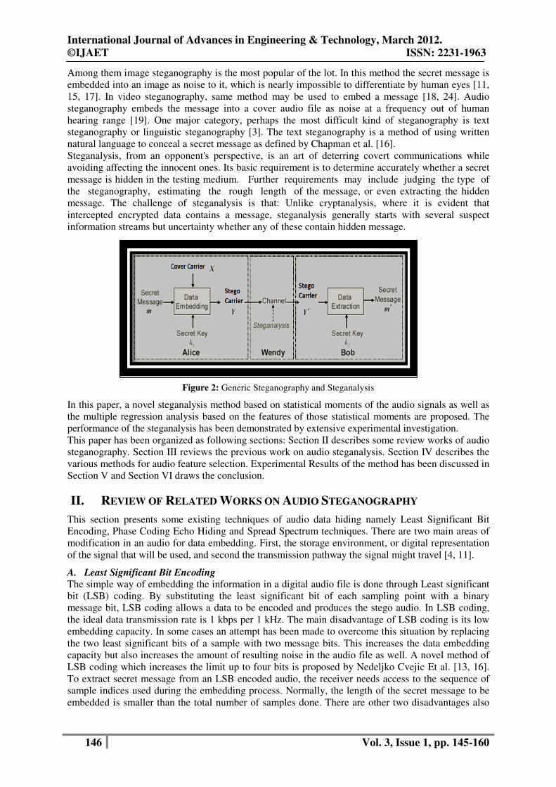
Steganalysis, from an opponent's perspective, is an art of deterring covert communications while
avoiding affecting the innocent ones. Its basic requirement is to determine accurately whether a secret
message is hidden in the testing medium. Further requirements may include judging the type of
the steganography, estimating the rough length of the message, or even extracting the hidden
message. The challenge of steganalysis is that: Unlike cryptanalysis, where it is evident that
intercepted encrypted data contains a message, steganalysis generally starts with several suspect
information streams but uncertainty whether any of these contain hidden message.
Fig. 1. Generic Steganography and Steganalysis
Figure 2: Generic Steganography and Steganalysis
In this paper, a novel steganalysis method based on statistical moments of the audio signals as well as
the multiple regression analysis based on the features of those statistical moments are proposed. The
performance of the steganalysis has been demonstrated by extensive experimental investigation.
This paper has been organized as following sections: Section II describes some review works of audio
steganography. Section III reviews the previous work on audio steganalysis. Section IV describes the
various methods for audio feature selection. Experimental Results of the method has been discussed in
Section V and Section VI draws the conclusion.
II. REVIEW OF RELATED WORKS ON AUDIO STEGANOGRAPHY
This section presents some existing techniques of audio data hiding namely Least Significant Bit
Encoding, Phase Coding Echo Hiding and Spread Spectrum techniques. There are two main areas of
modification in an audio for data embedding. First, the storage environment, or digital representation
of the signal that will be used, and second the transmission pathway the signal might travel [4, 11].
A. Least Significant Bit Encoding
The simple way of embedding the information in a digital audio file is done through Least significant
bit (LSB) coding. By substituting the least significant bit of each sampling point with a binary
message bit, LSB coding allows a data to be encoded and produces the stego audio. In LSB coding,
the ideal data transmission rate is 1 kbps per 1 kHz. The main disadvantage of LSB coding is its low
embedding capacity. In some cases an attempt has been made to overcome this situation by replacing
the two least significant bits of a sample with two message bits. This increases the data embedding
capacity but also increases the amount of resulting noise in the audio file as well. A novel method of
LSB coding which increases the limit up to four bits is proposed by Nedeljko Cvejic Et al. [13, 16].
To extract secret message from an LSB encoded audio, the receiver needs access to the sequence of
sample indices used during the embedding process. Normally, the length of the secret message to be
embedded is smaller than the total number of samples done. There are other two disadvantages also

International Journal of Advances in Engineering & Technology, March 2012.
©IJAET ISSN: 2231-1963
147 Vol. 3, Issue 1, pp. 145-160
associated LSB coding. The first one is that human ear is very sensitive and can often detect the
presence of single bit of noise into an audio file. Second disadvantage however, is that LSB coding is
not very robust. Embedded information will be lost through a little modification of the stego audio.
B. Phase Coding
Phase coding [11, 16] overcomes the disadvantages of noise induction method of audio
steganography. Phase coding designed based on the fact that the phase components of sound are not
as perceptible to the human ear as noise is. This method encodes the message bits as phase shifts in
the phase spectrum of a digital signal, achieving an inaudible encoding in terms of signal-to-noise
ratio. In figure 4 below original and encoded signal through phase coding method has been presented.
Figure 3: The original signal and encoded signal of phase coding technique.
Phase coding principles are summarized as under:
• The original audio signal is broken up into smaller segments whose lengths equal the size of
the message to be embedded.
• Discrete Fourier Transform (DFT) is applied to each segment to create a matrix of the phases
and Fourier transform magnitudes.
• Phase differences between adjacent segments are calculated next.
• Phase shifts between consecutive segments are easily detected. In other words, the absolute
phases of the segments can be changed but the relative phase differences between adjacent
segments must be preserved.
Thus the secret message is only inserted in the phase vector of the first signal segment as follows:
• A new phase matrix is created using the new phase of the first segment and the original phase
differences.
• Using the new phase matrix and original magnitude matrix, the audio signal is reconstructed
by applying the inverse DFT and by concatenating the audio segments.
To extract the secret message from the audio file, the receiver needs to know the segment length. The
receiver can extract the secret message through different reverse process.
The disadvantage associated with phase coding is that it has a low data embedding rate due to the fact
that the secret message is encoded in the first signal segment only. This situation can be overcome by
increasing the length of the signals segment which in turn increases the change in the phase relations
between each frequency component of the segment more drastically, making the encoding easier to
detect. Thus, the phase coding method is useful only when a small amount of data, such as a
watermark, needs to be embedded.
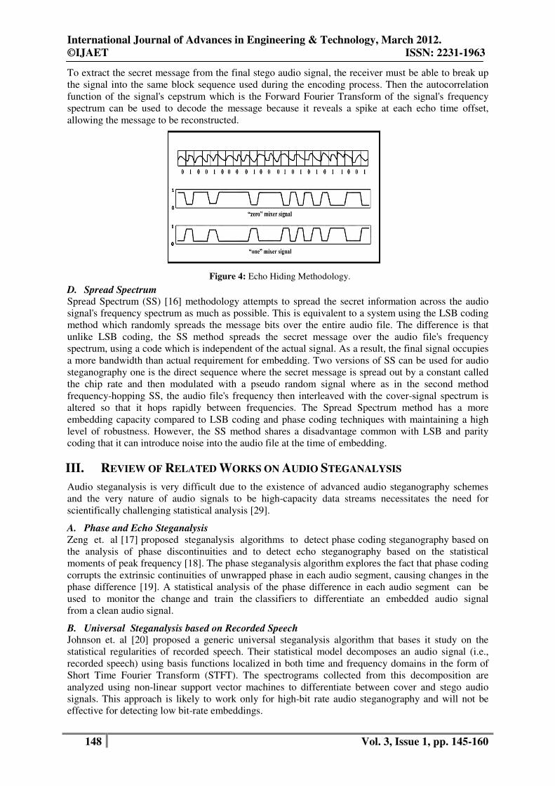
C. Echo Hiding In echo hiding [14, 15, 16] method information is embedded into an audio file by inducing an echo
into the discrete signal. Like the spread spectrum method, Echo Hiding method also has the advantage
of having high embedding capacity with superior robustness compared to the noise inducing methods.
If only one echo was produced from the original signal, only one bit of information could be encoded.
Therefore, the original signal is broken down into blocks before the encoding process begins. Once
the encoding process is completed, the blocks are concatenated back together to form the final signal.
Original Signal Encoded Signal
International Journal of Advances in Engineering & Technology, March 2012.
©IJAET ISSN: 2231-1963
148 Vol. 3, Issue 1, pp. 145-160
To extract the secret message from the final stego audio signal, the receiver must be able to break up
the signal into the same block sequence used during the encoding process. Then the autocorrelation
function of the signal's cepstrum which is the Forward Fourier Transform of the signal's frequency
spectrum can be used to decode the message because it reveals a spike at each echo time offset,
allowing the message to be reconstructed.
Figure 4: Echo Hiding Methodology.
D. Spread Spectrum Spread Spectrum (SS) [16] methodology attempts to spread the secret information across the audio
signal's frequency spectrum as much as possible. This is equivalent to a system using the LSB coding
method which randomly spreads the message bits over the entire audio file. The difference is that
unlike LSB coding, the SS method spreads the secret message over the audio file's frequency
spectrum, using a code which is independent of the actual signal. As a result, the final signal occupies
a more bandwidth than actual requirement for embedding. Two versions of SS can be used for audio
steganography one is the direct sequence where the secret message is spread out by a constant called
the chip rate and then modulated with a pseudo random signal where as in the second method
frequency-hopping SS, the audio file's frequency then interleaved with the cover-signal spectrum is
altered so that it hops rapidly between frequencies. The Spread Spectrum method has a more
embedding capacity compared to LSB coding and phase coding techniques with maintaining a high
level of robustness. However, the SS method shares a disadvantage common with LSB and parity
coding that it can introduce noise into the audio file at the time of embedding.
III. REVIEW OF RELATED WORKS ON AUDIO STEGANALYSIS
Audio steganalysis is very difficult due to the existence of advanced audio steganography schemes
and the very nature of audio signals to be high-capacity data streams necessitates the need for
scientifically challenging statistical analysis [29].
A. Phase and Echo Steganalysis
Zeng et. al [17] proposed steganalysis algorithms to detect phase coding steganography based on
the analysis of phase discontinuities and to detect echo steganography based on the statistical
moments of peak frequency [18]. The phase steganalysis algorithm explores the fact that phase coding
corrupts the extrinsic continuities of unwrapped phase in each audio segment, causing changes in the
phase difference [19]. A statistical analysis of the phase difference in each audio segment can be
used to monitor the change and train the classifiers to differentiate an embedded audio signal
from a clean audio signal.
B. Universal Steganalysis based on Recorded Speech Johnson et. al [20] proposed a generic universal steganalysis algorithm that bases it study on the
statistical regularities of recorded speech. Their statistical model decomposes an audio signal (i.e.,
recorded speech) using basis functions localized in both time and frequency domains in the form of
Short Time Fourier Transform (STFT). The spectrograms collected from this decomposition are
analyzed using non-linear support vector machines to differentiate between cover and stego audio
signals. This approach is likely to work only for high-bit rate audio steganography and will not be
effective for detecting low bit-rate embeddings.
International Journal of Advances in Engineering & Technology, March 2012.
©IJAET ISSN: 2231-1963
149 Vol. 3, Issue 1, pp. 145-160
C. Use of Statistical Distance Measures for Audio Steganalysis H. Ozer et. al [21] calculated the distribution of various statistical distance measures on cover audio
signals and stego audio signals vis--vis their versions without noise and observed them to be
statistically different. The authors employed audio quality metrics to capture the anomalies in the
signal introduced by the embedded data. They designed an audio steganalyzer that relied on the choice
of audio quality measures, which were tested depending on their perceptual or non-perceptual nature.
The selection of the proper features and quality measures was conducted using the (i) ANOVA test
[22] to determine whether there are any statistically significant differences between available
conditions and the (ii) SFS (Sequential Floating Search) algorithm that considers the inter-correlation
between the test features in ensemble [23]. Subsequently, two classifiers, one based on linear
regression and another based on support vector machines were used and also simultaneously
evaluated for their capability to detect stego messages embedded in the audio signals.
D. Audio Steganalysis based on Hausdorff Distance The audio steganalysis algorithm proposed by Liu et. al [24] uses the Hausdorff distance measure
[25] to measure the distortion between a cover audio signal and a stego audio signal. The algorithm
takes as input a potentially stego audio signal x and its de-noised version x as an estimate of the cover
signal. Both x and x are then subjected to appropriate segmentation and wavelet decomposition to
generate wavelet coefficients [26] at different levels of resolution. The Hausdorff distance values
between the wavelet coefficients of the audio signals and their de-noised versions are measured. The
statistical moments of the Hausdorff distance measures are used to train a classifier on the difference
between cover audio signals and stego audio signals with different content loadings.
E. Audio Steganalysis for High Complexity Audio Signals More recently, Liu et. al [27] propose the use of stream data mining for steganalysis of audio signals
of high complexity. Their approach extracts the second order derivative based Markov transition
probabilities and high frequency spectrum statistics as the features of the audio streams. The
variations in the second order derivative based features are explored to distinguish between the cover
and stego audio signals. This approach also uses the Mel-frequency cepstral coefficients [28], widely
used in speech recognition, for audio steganalysis. Recently two new methods of audio steganalysis of
spread spectrum information hiding has been proposed in [31-32].
IV. AUDIO FEATURE SELECTION
In this section audio quality measures in terms of moments up to 7th order both statistical and
invariants has been investigated for the purpose of audio steganalysis. Various moments of the audio
signals are sensitive to the presence of a steganographic message embedding. Moments based features
have been extracted for steganalytic measure in such a way that reflect the quality of distorted or
degraded audio signal vis-à-vis its original in an accurate, consistent and monotonic way. Such a
measure, in the context of steganalysis, should respond to the presence of hidden message with
minimum error, should work for a large variety of embedding methods, and its reaction should be
proportional to the embedding strength.
A. Moments based Audio feature
To construct the features of both cover and stego or suspicious audios moments of the audio series has
been computed. In mathematics, a moment is, loosely speaking, a quantitative measure of the shape of
a set of points. The "second moment", for example, is widely used and measures the "width" (in a
particular sense) of a set of points in one dimension or in higher dimensions measures the shape of a
cloud of points as it could be fit by an ellipsoid. Other moments describe other aspects of
a distribution such as how the distribution is skewed from its mean, or peaked. There are two ways of
viewing moments [30], one based on statistics and one based on arbitrary functions such as f(x) or f(x,
y). As a result moments can be defined in more than one way.
Statistical view Moments are the statistical expectation of certain power functions of a random variable. The most
common moment is the mean which is just the expected value of a random variable as given in
equation 1.
International Journal of Advances in Engineering & Technology, March 2012.
©IJAET ISSN: 2231-1963
150 Vol. 3, Issue 1, pp. 145-160
(4)
E[ ] ( )X x f x dxµ
∞
−∞
= = ∫ (1)
Where f(x) is the probability density function of continuous random variable X. More generally,
moments of order p = 0, 1, 2, … can be calculated as mp = E [Xp].These are sometimes referred to as
the raw moments. There are other kinds of moments that are often useful.
One of these is the central moments µp = E [(X–µ)p].The best known central moment is the second,
which is known as the variance given in equation 2.
2 2 2
2 1( ) ( )x f x dx mσ µ µ= − = −∫
(2)
Two less common statistical measures, skewness and kurtosis, are based on the third and fourth
central moments. The use of expectation assumes that the pdf is known. Moments are easily extended
to two or more dimensions as shown in equation 3.
E[ ] ( , )p q p q
pqm X Y x y f x y dx dy= = ∫∫
(3)
Here f(x, y) is the joint pdf.
Estimation However, moments are easy to estimate from a set of measurements, xi. The p-th moment is estimated
as given in equation 4 and 5.
1
1 Np
p i
i
m xN =
= ∑
(Often 1/N is left out of the definition) and the p-th central moment is estimated as
1( ) p
p i
i
x xN
µ = −∑ (5)
is the average of the measurements, which is the usual estimate of the mean. The second central
moment gives the variance of a set of data s2 = µ2.For multidimensional distributions, the first and
second order moments give estimates of the mean vector and covariance matrix. The order of
moments in two dimensions is given by p+q, so for moments above 0, there is more than one of a
given order. For example, m20, m11, and m02 are the three moments of order 2.
Non-statistical view This view is not based on probability and expected values, but most of the same ideas still hold. For
any arbitrary function f(x), one may compute moments using the equation 6 or for a 2-D function
using the equation 7.
( )p
pm x f x dx
∞
−∞
= ∫ (6)
( , )p q
pqm x y f x y dx dy= ∫∫ (7)
Notice now that to find the mean value of f(x), one must use m1/m0, since f(x) is not normalized to area
1 like the pdf. Likewise, for higher order moments it is common to normalize these moments by
dividing by m0 (or m00). This allows one to compute moments which depend only on the shape and
not the magnitude of f(x). The result of normalizing moments gives measures which contain
information about the shape or distribution (not probability dist.) of f(x).

International Journal of Advances in Engineering & Technology, March 2012.
©IJAET ISSN: 2231-1963
151 Vol. 3, Issue 1, pp. 145-160
(10)
Digital approximation For digitized data (including images) we must replace the integral with a summation over the domain
covered by the data. The 2-D approximation is written in equation 8.
1 1
1 1
( , )
( , )
M Np q
pq i j i j
i j
M Np q
i j
m f x y x y
f i j i j
= =
= =
=
=
∑∑
∑∑ (8)
If f(x, y) is a binary image function of an object, the area is m00, the x and y centroids are 10 00/x m m=
and 01 00/y m m= .
Invariance
In many applications such as shape recognition, it is useful to generate shape features which are
independent of parameters which cannot be controlled in an image. Such features are called invariant
features. There are several types of invariance. For example, if an object may occur in an arbitrary
location in an image, then one needs the moments to be invariant to location. For binary connected
components, this can be achieved simply by using the central moments, µpq. If an object is not at a
fixed distance from a fixed focal length camera, then the sizes of objects will not be fixed. In this
case size invariance is needed. This can be achieved by normalizing the moments as given in
equation 9.
00
, where ½( ) 1.pq
pqp q
γ
µη γ
µ= = + +
(9)
The third common type of invariance is rotation invariance. This is not always needed, for example if
objects always have a known direction as in recognizing machine printed text in a document. The
direction can be established by locating lines of text.
M.K. Hu derived a transformation of the normalized central moments to make the resulting moments
rotation invariant as given in equation 10.

International Journal of Advances in Engineering & Technology, March 2012.
©IJAET ISSN: 2231-1963
152 Vol. 3, Issue 1, pp. 145-160
B. Regression based Analysis Method In statistics, regression analysis includes any techniques for modeling and analyzing several variables,
when the focus is on the relationship between a dependent variable and one or more independent
variables. More specifically, regression analysis helps one understand how the typical value of the
dependent variable changes when any one of the independent variables is varied, while the other
independent variables are held fixed. In all cases, the estimation target is a function of the independent
variables called the regression function.In regression analysis, it is also of interest to characterize the
variation of the dependent variable around the regression function, which can be described by a
probability distribution. Regression analysis is widely used for prediction and forecasting, where its
use has substantial overlap with the field of machine learning. Regression analysis is also used to
understand which among the independent variables are related to the dependent variable, and to
explore the forms of these relationships. In restricted circumstances, regression analysis can be used
to infer causal relationships between the independent and dependent variables. A large body of
techniques for carrying out regression analysis has been developed. Familiar methods such as linear
regression and ordinary least squares regression are parametric, in that the regression function is
defined in terms of a finite number of unknown parameters that are estimated from the data.
Nonparametric regression refers to techniques that allow the regression function to lie in a specified
set of functions, which may be infinite-dimensional. The performance of regression analysis methods
in practice depends on the form of the data-generating process, and how it relates to the regression
approach being used. Since the true form of the data-generating process is in general not known,
regression analysis often depends to some extent on making assumptions about this process. These
assumptions are sometimes (but not always) testable if a large amount of data is available. Regression
models for prediction are often useful even when the assumptions are moderately violated, although
they may not perform optimally. However, in many applications, especially with small effects or
questions of causality based on observational data, regression methods give misleading results.
Regression models: Regression models involve the following variables
� The unknown parameters denoted as β; this may be a scalar or a vector.
� The independent variables X.
� The dependent variable, Y.
In various fields of application, different terminologies are used in place of dependent and
independent variables.
A regression model relates Y to a function of X and β as given in equation 11.
The approximation is usually formalized as E(Y | X) = f(X, β). To carry out regression analysis, the
form of the function f must be specified. Sometimes the form of this function is based on knowledge
about the relationship between Y and X that does not rely on the data. If no such knowledge is
available, a flexible or convenient form for f is chosen.
Linear regression: In linear regression, the model specification is that the dependent variable, yi is
a linear combination of the parameters (but need not be linear in the independent variables). For
example, in simple linear regression for modeling n data points there is one independent variable: xi,
and two parameters, β0 and β1:
Yi = β0+β1xi+εi , i =1,…….,n.-----(12)
In multiple linear regressions, there are several independent variables or functions of independent
variables. For example, adding a term in xi2
to the preceding regression gives:
Yi = β0+β1xi+β2 xi2+ εi , i =1,…….,n.--------(13)
This is still linear regression; although the expression on the right hand side is quadratic in the
independent variable xi, it is linear in the parameters β0, β1 and β2.In both cases, εi is an error term and
the subscript i indexes a particular observation. Given a random sample from the population, we
estimate the population parameters and obtain the sample linear regression model:
Ŷi= β0+β1xi ------------ (14)
International Journal of Advances in Engineering & Technology, March 2012.
©IJAET ISSN: 2231-1963
153 Vol. 3, Issue 1, pp. 145-160
The residual, ei = Yi - Ŷi the difference between the value of the dependent variable predicted by the
model, Ŷi and the true value of the dependent variable Yi.
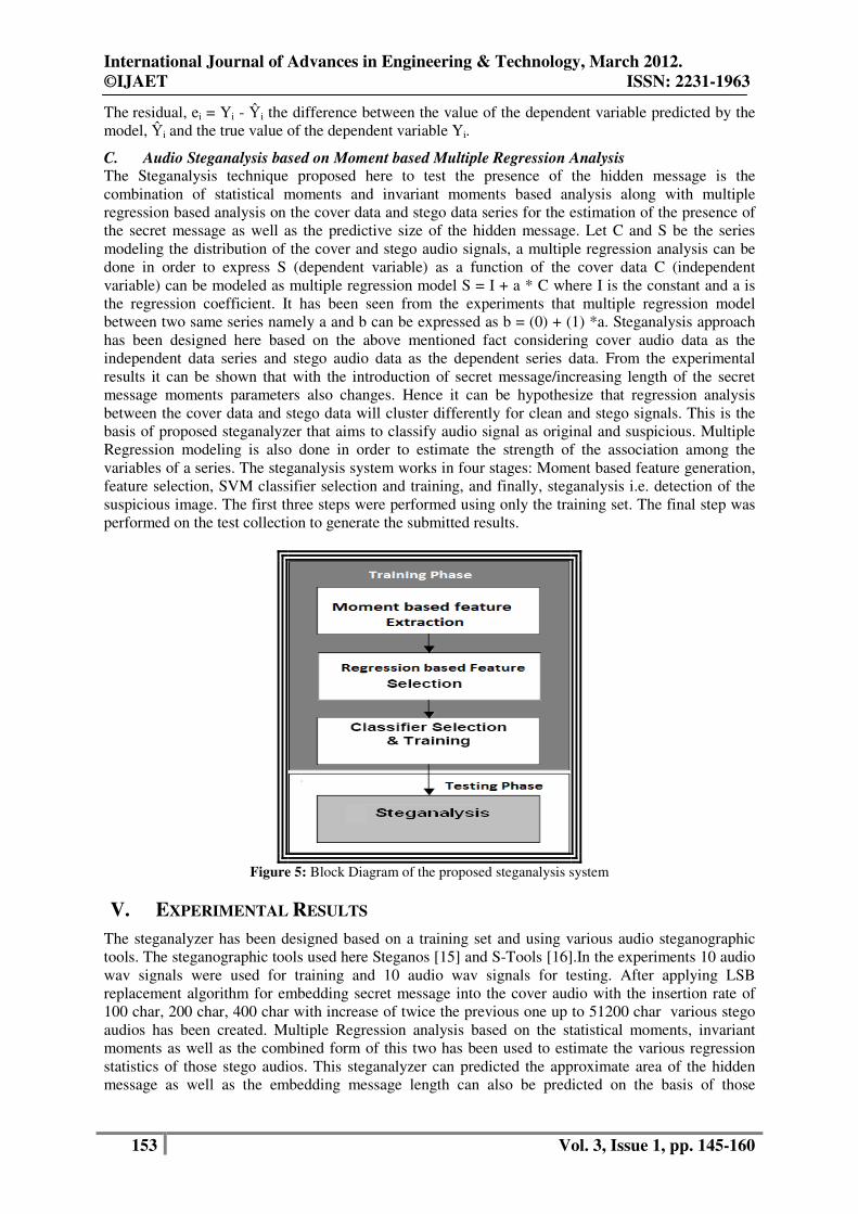
C. Audio Steganalysis based on Moment based Multiple Regression Analysis The Steganalysis technique proposed here to test the presence of the hidden message is the
combination of statistical moments and invariant moments based analysis along with multiple
regression based analysis on the cover data and stego data series for the estimation of the presence of
the secret message as well as the predictive size of the hidden message. Let C and S be the series
modeling the distribution of the cover and stego audio signals, a multiple regression analysis can be
done in order to express S (dependent variable) as a function of the cover data C (independent
variable) can be modeled as multiple regression model S = I + a * C where I is the constant and a is
the regression coefficient. It has been seen from the experiments that multiple regression model
between two same series namely a and b can be expressed as b = (0) + (1) *a. Steganalysis approach
has been designed here based on the above mentioned fact considering cover audio data as the
independent data series and stego audio data as the dependent series data. From the experimental
results it can be shown that with the introduction of secret message/increasing length of the secret
message moments parameters also changes. Hence it can be hypothesize that regression analysis
between the cover data and stego data will cluster differently for clean and stego signals. This is the
basis of proposed steganalyzer that aims to classify audio signal as original and suspicious. Multiple
Regression modeling is also done in order to estimate the strength of the association among the
variables of a series. The steganalysis system works in four stages: Moment based feature generation,
feature selection, SVM classifier selection and training, and finally, steganalysis i.e. detection of the
suspicious image. The first three steps were performed using only the training set. The final step was
performed on the test collection to generate the submitted results.
Figure 5: Block Diagram of the proposed steganalysis system
V. EXPERIMENTAL RESULTS
The steganalyzer has been designed based on a training set and using various audio steganographic
tools. The steganographic tools used here Steganos [15] and S-Tools [16].In the experiments 10 audio
wav signals were used for training and 10 audio wav signals for testing. After applying LSB
replacement algorithm for embedding secret message into the cover audio with the insertion rate of
100 char, 200 char, 400 char with increase of twice the previous one up to 51200 char various stego
audios has been created. Multiple Regression analysis based on the statistical moments, invariant
moments as well as the combined form of this two has been used to estimate the various regression
statistics of those stego audios. This steganalyzer can predicted the approximate area of the hidden
message as well as the embedding message length can also be predicted on the basis of those
International Journal of Advances in Engineering & Technology, March 2012.
©IJAET ISSN: 2231-1963
154 Vol. 3, Issue 1, pp. 145-160
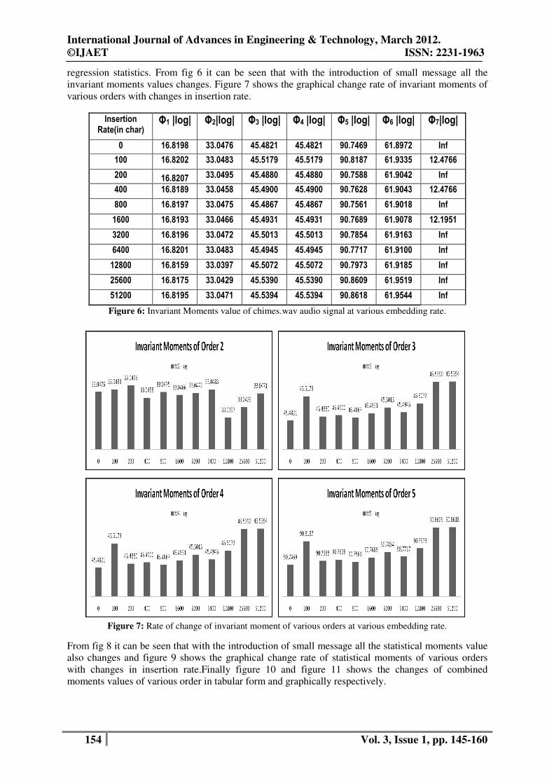
regression statistics. From fig 6 it can be seen that with the introduction of small message all the
invariant moments values changes. Figure 7 shows the graphical change rate of invariant moments of
various orders with changes in insertion rate.
Insertion Rate(in char)
Φ1 |log| Φ2|log| Φ3 |log| Φ4 |log| Φ5 |log| Φ6 |log| Φ7|log|
0 16.8198 33.0476 45.4821 45.4821 90.7469 61.8972 Inf
100 16.8202 33.0483 45.5179 45.5179 90.8187 61.9335 12.4766
200 16.8207 33.0495 45.4880 45.4880 90.7588 61.9042 Inf
400 16.8189 33.0458 45.4900 45.4900 90.7628 61.9043 12.4766
800 16.8197 33.0475 45.4867 45.4867 90.7561 61.9018 Inf
1600 16.8193 33.0466 45.4931 45.4931 90.7689 61.9078 12.1951
3200 16.8196 33.0472 45.5013 45.5013 90.7854 61.9163 Inf
6400 16.8201 33.0483 45.4945 45.4945 90.7717 61.9100 Inf
12800 16.8159 33.0397 45.5072 45.5072 90.7973 61.9185 Inf
25600 16.8175 33.0429 45.5390 45.5390 90.8609 61.9519 Inf
51200 16.8195 33.0471 45.5394 45.5394 90.8618 61.9544 Inf
Figure 6: Invariant Moments value of chimes.wav audio signal at various embedding rate.
Figure 7: Rate of change of invariant moment of various orders at various embedding rate.
From fig 8 it can be seen that with the introduction of small message all the statistical moments value
also changes and figure 9 shows the graphical change rate of statistical moments of various orders
with changes in insertion rate.Finally figure 10 and figure 11 shows the changes of combined
moments values of various order in tabular form and graphically respectively.

International Journal of Advances in Engineering & Technology, March 2012.
©IJAET ISSN: 2231-1963
155 Vol. 3, Issue 1, pp. 145-160
Insertion Rate (in char)
M1 |log| M2 |log| M3 |log| M4 |log| M5 |log| M6 |log| M7 |log|
0 Inf 5.0144 10.7782 6.7931 10.0539 7.5902 9.9484
100 Inf 5.0144 10.7795 6.7931 10.0543 7.5902 9.9485
200 Inf 5.0143 10.7790 6.7931 10.0543 7.5902 9.9486
400 Inf 5.0144 10.7789 6.7931 10.0540 7.5902 9.9484
800 Inf 5.0144 10.7808 6.7931 10.0544 7.5902 9.9486
1600 Inf 5.0144 10.7793 6.7932 10.0539 7.5904 9.9499
3200 Inf 5.0144 10.7844 6.7932 10.0570 7.5905 9.9505
6400 Inf 5.0144 10.7870 6.7932 10.0573 7.5905 9.9506
12800 Inf 5.0144 10.7800 6.7931 10.0540 7.5902 9.9483
25600 Inf 5.0144 10.7833 6.7932 10.0548 7.5903 9.9487
51200 Inf 5.0144 10.7782 6.7932 10.0541 7.5903 9.9487
Figure 8: Statistical Moments value of chimes.wav audio signal at various embedding rate.
Figure 9: Rate of change of statistical moment of various orders at various embedding rate.

International Journal of Advances in Engineering & Technology, March 2012.
©IJAET ISSN: 2231-1963
156 Vol. 3, Issue 1, pp. 145-160
Insertion Rate (in char)
CM1 |log|
CM2 |log|
CM3 |log|
CM4 |log|
CM5 |log| CM6 |log|
CM7 |log|
CAVGM
0 Inf 38.0620 56.2603 52.2752 100.8008 69.4874 Inf 39.7357
100 Inf 38.0627 56.2974 52.3110 100.8730 69.5237 22.4251 39.7585
200 Inf 38.0638 56.2670 52.2811 100.8131 69.4944 Inf 39.7399
400 Inf 38.0602 56.2689 52.2831 100.8168 69.4945 22.4250 39.7404
800 Inf 38.0619 56.2675 52.2798 100.8105 69.4920 Inf 39.7390
1600 Inf 38.0610 56.2724 52.2863 100.8228 69.4982 22.1450 39.7426
3200 Inf 38.0616 56.2857 52.2945 100.8424 69.5068 Inf 39.7489
6400 Inf 38.0627 56.2815 52.2877 100.8290 69.5005 Inf 39.7452
12800 Inf 38.0541 56.2872 52.3003 100.8513 69.5087 Inf 39.7502
25600 Inf 38.0573 56.3223 52.3322 100.9157 69.5422 Inf 39.7712
51200 Inf 38.0615 56.3176 52.3326 100.9159 69.5447 Inf 39.7715
Figure 10: Combined Moments value of chimes audio signal at various embedding rate.
Figure 11: Rate of change of combined moments of various orders at various embedding rate.

International Journal of Advances in Engineering & Technology, March 2012.
©IJAET ISSN: 2231-1963
157 Vol. 3, Issue 1, pp. 145-160
Figure 12: Rate of Change of Average Combined Moments value at various insertion rates
To build the classes of Cover Audio signals Combined Moment values of the original 10 audio signals
(chimes.wav, heartbeat.wav etc) are inserted in the database. Next step is to produce stego audio
signals with those original audio signals with random bits and different rates in another database.
Original audio signals database with various moments values are used for training set from which the
classifiers are tuned. With help of this an incoming audio signal can be classified as stego or cover
audio signal. Figure 11 shows the rate of changes of average combined moment values at various
insertion rate where as fig 12 shows the combined moments value at the various segments of the
original audio signal chimes.wav and also show the changes of moments value after embedding 100
char in segment1. From the figure it can be seen that moments value has been changed in segment1
with the introduction of data where as segment2, segment3 and segment 4 parameters are remain un-
changed.
Figure 13: Combined Moments value at various audio segment of the original and stego audio
Thus it can be concluded that secret data has been embedded in segment1 portion of the cover audio
signal. Next step is to predict the length of the hidden message. The classifier is trained with the
values of Combined Moments of order 2, 3, 4, 5 and 6 of the original audio signal and stego signals
with different embedding rate in order to form a relation between the embedding capacity and the
combined moment values order 2, 3, 4, 5 and 6. Insertion rate can be computed from the various
International Journal of Advances in Engineering & Technology, March 2012.
©IJAET ISSN: 2231-1963
158 Vol. 3, Issue 1, pp. 145-160
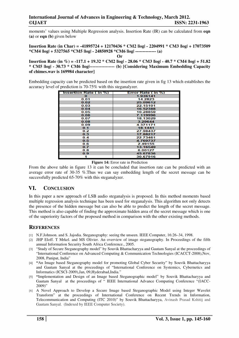
moments’ values using Multiple Regression analysis. Insertion Rate (IR) can be calculated from eqn
(a) or eqn (b) given below
Insertion Rate (in Char) = -41895724 + 12170436 * CM2 |log| - 2204991 * CM3 |log| + 17073509
*CM4 |log| + 5327565 *CM5 |log| - 24850928 *CM6 |log| -------------- (a)
Or
Insertion Rate (in %) = -117.1 + 19.32 * CM2 |log| - 28.06 * CM3 |log| - 40.7 * CM4 |log| + 51.82
* CM5 |log| - 30.73 * CM6 |log|----------------- (b) [Considering Maximum Embedding Capacity
of chimes.wav is 169984 character]
Embedding capacity can be predicted based on the insertion rate given in fig 13 which establishes the
accuracy level of prediction is 70-75% with this steganalyzer.
Figure 14: Error rate in Prediction
From the above table in figure 13 it can be concluded that insertion rate can be predicted with an
average error rate of 30-35 %.Thus we can say embedding length of the secret message can be
successfully predicted 65-70% with this steganalyzer.
VI. CONCLUSION
In this paper a new approach of LSB audio steganalysis is proposed. In this method moments based
multiple regression analysis technique has been used for steganalysis. This algorithm not only detects
the presence of the hidden message but can also be able to predict the length of the secret message.
This method is also capable of finding the approximate hidden area of the secret message which is one
of the superiority factors of the proposed method in comparison with the other existing methods.
REFERENCES
[1] N.F.Johnson. and S. Jajodia. Steganography: seeing the unseen. IEEE Computer, 16:26–34, 1998.
[2] JHP Eloff. T Mrkel. and MS Olivier. An overview of image steganography. In Proceedings of the fifth
annual Information Security South Africa Conference., 2005.
[3] “Study of Secure Steganography model” by Souvik Bhattacharyya and Gautam Sanyal at the proceedings of
“International Conference on Advanced Computing & Communication Technologies (ICACCT-2008),Nov,
2008, Panipat, India”
[4] “An Image based Steganography model for promoting Global Cyber Security” by Souvik Bhattacharyya
and Gautam Sanyal at the proceedings of “International Conference on Systemics, Cybernetics and
Informatics (ICSCI-2009),Jan, 09,Hyderabad,India.”
[5] “Implementation and Design of an Image based Steganographic model” by Souvik Bhattacharyya and
Gautam Sanyal at the proceedings of “ IEEE International Advance Computing Conference “(IACC-
2009)” [6] A Novel Approach to Develop a Secure Image based Steganographic Model using Integer Wavelet
Transform” at the proceedings of International Conference on Recent Trends in Information,
Telecommunication and Computing (ITC 2010)” by Souvik Bhattacharyya, Avinash Prasad Kshitij and
Gautam Sanyal. (Indexed by IEEE Computer Society).

International Journal of Advances in Engineering & Technology, March 2012.
©IJAET ISSN: 2231-1963
159 Vol. 3, Issue 1, pp. 145-160
[7] C. Kraetzer and J. Dittmann, “Pros and Cons of Mel cepstrum based Audio Steganalysis using SVM
Classification,” Lecture Notes in Computer Science, vol. 4567, pp. 359 – 377, January 2008.
[8] W. Zeng, H. Ai and R. Hu, “A Novel Steganalysis Algorithm of Phase Coding in Audio Signal,”
Proceedings of the 6th International Conference on Advanced Language Processing and Web Information
Technology, pp. 261 – 264, August 2007.
[9] W. Zeng, H. Ai and R. Hu, “An Algorithm of Echo Steganalysis based on Power Cepstrum and Pattern
Classification,” Proceedings of the International Conference on Information and Automation, pp. 1667 –
1670, June 2008.
[10] M. K. Johnson, S. Lyu, H. Farid, “Steganalysis of Recorded Speech,” Proceedings of Conference on
Security, Steganography and Watermarking of Multimedia, Contents VII, vol. 5681, SPIE, pp. 664– 672,
May 2005.
[11] H. Ozer, I. Avcibas, B. Sankur and N. D. Memon, “Steganalysis of Audio based on Audio Quality Metrics,”
Proceedings of the Conference on Security, Steganography and Watermarking of Multimedia, Contents V,
vol. 5020, SPIE, pp. 55 – 66, January 2003.
[12] Y. Liu, K. Chiang, C. Corbett, R. Archibald, B. Mukherjee and D. Ghosal, “A Novel Audio Steganalysis
based on Higher-Order Statistics of a Distortion Measure with Hausdorff Distance,” Lecture Notes in
Computer Science, vol. 5222, pp. 487 -501, September 2008.
[13] D. P. Huttenlocher, G. A. Klanderman and W. J. Rucklidge, “Comparing Images using Hausdorff
Distance,” IEEE Transactions on Pattern Analysis and Machine Intelligence, vol. 19, no. 9, pp. 850– 863,
September 1993.
[14] T. Holotyak, J. Fridrich and S. Voloshynovskiy, “Blind Statistical Steganalysis of Additive Steganography
using Wavelet Higher Order Statistics,” Lecture Notes in Computer Science, vol. 3677, pp. 273 – 274,
September 2005.
[15] N. Memon I. Avcibas and B. Sankur. Steganalysis using image quality metrics. Signal Processing., IEEE
Transactions on Image Processing,12(2):221-229, 2003.
[16] M. Goljan J. Fridrich and D. Hogea. Attacking the outguess. In Proceedings of 2002 ACM Workshop on
Multimedia and Security,ACM Press., 2002. [17] W. Zeng, H. Ai and R. Hu, “A Novel Steganalysis Algorithm of Phase Coding in Audio Signal,”
Proceedings of the 6th International Conference on Advanced Language Processing and Web Information
Technology, pp. 261 – 264, August 2007.
[18] W. Zeng, H. Ai and R. Hu, “An Algorithm of Echo Steganalysis based on Power Cepstrum and Pattern
Classification,” Proceedings of the International Conference on Information and Automation, pp. 1667 –
1670, June 2008.
[19] Paraskevas and E. Chilton, “Combination of Magnitude and Phase Statistical Features for Audio
Classification,” Acoustical Research Letters Online, Acoustical Society of America, vol. 5, no. 3, pp. 111 –
117, July 2004.
[20] M. K. Johnson, S. Lyu, H. Farid, “Steganalysis of Recorded Speech,” Proceedings of Conference on
Security, Steganography and Watermarking of Multimedia, Contents VII, vol. 5681, SPIE, pp. 664– 672,
May 2005.
[21] H. Ozer, I. Avcibas, B. Sankur and N. D. Memon, “Steganalysis of Audio based on Audio Quality Metrics,”
Proceedings of the Conference on Security, Steganography and Watermarking of Multimedia, Contents V,
vol. 5020, SPIE, pp. 55 – 66, January 2003.
[22] A.C. Rencher, Methods of Multivariate Data Analysis, 2nd Edition, John Wiley, New York, NY, March
2002.
[23] P. Pudil, J. Novovicova and J. Kittler, “Floating Search Methods in Feature Selection,” Pattern Recognition
Letters, vol. 15, no. 11, pp. 1119 – 1125, November 1994.
[24] Y. Liu, K. Chiang, C. Corbett, R. Archibald, B. Mukherjee and D. Ghosal, “A Novel Audio Steganalysis
based on Higher-Order Statistics of a Distortion Measure with Hausdorff Distance,” Lecture Notes in
Computer Science, vol. 5222, pp. 487 -501, September 2008.
[25] P. Huttenlocher, G. A. Klanderman and W. J. Rucklidge, “Comparing Images using Hausdorff Distance,”
IEEE Transactions on Pattern Analysis and Machine Intelligence, vol. 19, no. 9, pp. 850– 863, September
1993.
[26] T. Holotyak, J. Fridrich and S. Voloshynovskiy, “Blind Statistical Steganalysis of Additive Steganography
using Wavelet Higher Order Statistics,” Lecture Notes in Computer Science, vol. 3677, pp. 273 – 274,
September 2005.
[27] I.Avcibas, “Audio Steganalysis with Content-independent Distortion Measures,” IEEE Signal Processing
Letters, vol. 13, no. 2, pp. 92 – 95, February 2006.
[28] Q. Liu, A. H. Sung and M. Qiao, “Novel Stream Mining for Audio Steganalysis,” Proceedings of the 17th
ACM International Conference on Multimedia, pp. 95 – 104, Beijing, China, October 2009.
International Journal of Advances in Engineering & Technology, March 2012.
©IJAET ISSN: 2231-1963
160 Vol. 3, Issue 1, pp. 145-160
[29] C. Kraetzer and J. Dittmann, “Pros and Cons of Mel cepstrum based Audio Steganalysis using SVM
Classification,” Lecture Notes in Computer Science, vol. 4567, pp. 359 – 377, January 2008.
[30] MOMENTS IN IMAGE PROCESSING Bob Bailey Nov. 2002
[31] Audio steganalysis of spread spectrum hiding based on statistical moment by Zhang Kexin at the
proceedings of 2nd International Conference on Signal Processing Systems (ICSPS), 2010.
[32] Audio steganalysis of spread spectrum information hiding based on statistical moment and distance metric
by Wei Zeng, Ruimin Hu and Haojun Ai at Multimedia Tools and Applications Volume 55, Number 3,
525-556.
AUTHORS
Souvik Bhattacharyya received his B.E. degree in Computer Science and Technology from B.E.
College, Shibpur, India, presently known as Bengal Engineering and Science University (BESU)
and M.Tech degree in Computer Science and Engineering from National Institute of Technology,
Durgapur, India. Currently he is working as an Assistant Professor in Computer Science and
Engineering Department at University Institute of Technology, The University of Burdwan. He has
more than 30 research publication in his credit. His areas of interest are Natural Language
Processing, Network Security and Image Processing.
Gautam Sanyal has received his B.E and M.Tech degree National Institute of Technology
(NIT), Durgapur, India. He has received Ph.D (Engg.) from Jadavpur University, Kolkata, India,
in the area of Robot Vision. He possesses an experience of more than 25 years in the field of
teaching and research. He has published nearly 72 papers in International and National Journals /
Conferences. Three Ph.Ds (Engg) have already been awarded under his guidance. At present he
is guiding six Ph.Ds scholars in the field of Steganography, Cellular Network, High Performance
Computing and Computer Vision. He has guided over 10 PG and 100 UG thesis. His research interests include
Natural Language Processing, Stochastic modeling of network traffic, High Performance Computing, Computer
Vision. He is presently working as a Professor in the department of Computer Science and Engineering and also
holding the post of Dean (Students’ Welfare) at National Institute of Technology, Durgapur, India. He is a
member of IEEE also.
Top Related