


Languages
Pages
Legal


ASSET PRICES AND MONETARY POLICY:
WEALTH EFFECTS ON CONSUMPTION
JOSÉ MARTINS BARATA Professor, ISEG, Technical University of Lisbon
Research Director at CIEF, ISEG, Technical University of Lisbon
LUÍS MIGUEL PACHECO
Research Assistant at CIEF
Assistant at Universidade Portucalense, Oporto
Paper for 20th Symposium on Banking and Monetary Economics
June 5 and 6, 2003 held in University of Birmingham
(organised by GdR 0098 of CNRS – France)
CIEF – Centro de Investigação sobre Economia Financeira Rua Miguel Lupi, 20, 1200-781 Lisbon PORTUGAL
e-mail: [email protected]
______________________________________________________________________ Financial support granted by the Fundação para a Ciência e Tecnologia (FCT) and the Programa POCTI is gratefully acknowledged. The usual disclaimer applies. ______________________________________________________________________
Lisbon, February 2003

1
ASSET PRICES AND MONETARY POLICY:
WEALTH EFFECTS ON CONSUMPTION
JOSÉ MARTINS BARATA Professor, ISEG, Technical University of Lisbon
Research Director at CIEF, ISEG, Technical University of Lisbon
LUÍS MIGUEL PACHECO Research Assistant at CIEF
Assistant at Universidade Portucalense, Oporto
ABSTRACT
The aim of this paper is to test a model explaining private consumption as a function of income and wealth (financial assets plus real estate), with data from European Union (EU) countries. We know that income explains a large part of consumption as well as wealth, but concerning the effects of the latter, mainly those of changes on financial asset prices, few is known for Europe. In a general way, and according to the literature, wealth effects are less significant in continental Europe, due to the less advanced financial deregulation degree and household stock ownership, when compared with the USA or the United Kingdom. On the other hand, housing wealth effects on consumption would be more pronounced in Europe. To examine how recent developments in stock markets and housing prices may have affected consumption behaviour, we consider for the different countries a set of consumption equations that include variables related to asset prices. After studying the variables’ stationarity properties, we estimate a model with a common error-correction formulation, with the long-run relationship - having terms in the variables for which we found significant cointegrating vectors - nested in a short-run equation. We found an implied elasticity of consumption with respect to real equities prices at around two per cent and, when there is available data, an implied elasticity of consumption with respect to real residential prices between ten and twenty per cent. This weak effect of stock prices on consumer spending is broadly consistent with life cycle saving and a modest wealth effect. Nevertheless, it is still worthy to do a further study of the effects of stock market and residential wealth (and its fluctuations) on consumption and output of the different countries. The complete study of those differences and its magnitude is important even for the definition of the monetary policy by the European Central Bank (ECB) and to answer the question if it should consider asset prices in its decisions. The research presented here is a first essay preceding a deeper work on this subject, concerning economies of the EU. After this exercise we think that there is scope for future analysis on this matter that attempts to better explain the connection between asset prices and consumer spending.

2
1. Introduction
The aim of this paper is to test a model explaining private consumption as a function of
income and wealth (financial assets plus real estate), with data from European Union
(EU) countries.
We know that income explains a large part of consumption as well as wealth, but
concerning the effects of the latter, mainly those of changes on financial asset prices,
few is known for Europe.
In recent years, the interest of studying the effect of stock exchange prices fluctuations
arose mainly as consequence of a large involvement of families in stock exchanges,
placing their savings in equities that depreciated strongly after the collapse of the so
called “new economy” boom. A fear that this collapse might imply a high decrease of
private consumption, as well as a reduction of investment and income, has thrown the
attention of economists towards the analysis of these wealth effects, mainly in the
United States of America (USA).
Beyond financial assets, we think that real estate prices may also influence private
consumption and this may occur more when interest rates are low (mortgage credit
cheaper) and stock ownership is viewed as too risky, hence dangerous for savings
placements.
The research we present here is a first essay preceding a deeper work on this subject,
concerning economies of the EU. Now we take only data from five States, that we
consider a meaningful sample: two core economies of the continental EU (France and
Germany); two small and peripheral economies (Finland and Portugal) and an economy
of the EU country that seems to approach more the American patterns (United
Kingdom). We expect results that will suggest the better path to follow with further
research.
In the following section we discuss the theoretical background pertinent to our research.
The subsequent sections present the methodology, the data and the empirical results.
The last section concludes.

3
2. Theoretical background and some earlier evidence
We depart from the “life cycle theory” of Modigliani (Ando and Modigliani [1963] and
Modigliani [1971]) as a seminal paradigm concerning the explanation of consumption
as a variable depending on wealth, beyond income. In that framework, household
planned consumption (Ct*) is a function of total resources, which are net financial
wealth at the beginning of the period (Wt-1) and human wealth (Ht). Therefore, planned
consumption can be expressed as:
Ct* = F( Wt-1, Ht ) (1)
There are some pitfalls in estimating that equation: i) planned consumption does not
always equal actual consumption due to lags in adjustment, which suggests to use an
error correction approach; ii) human wealth is not observable, so instead of it a proxy is
taken, let it be some measure of income. So, traditionally the wealth effect has been
measured by estimating aggregate time-series regressions of the form1:
Ct = ? + ? 1.Wt + ? 2.Yt + ut (2)
Where C stand for household actual consumer spending, Y represents disposable
income and W is household net worth or wealth. ? 1 and ? 2 are, respectively, the
marginal propensities to consume out of wealth and disposable income, respectively. A
widespread empirical practice is to introduce lags and separate wealth into different
categories, as stock market wealth or housing and property wealth.
Modigliani (1971) advocates the significance of wealth effects on consumption, and
earlier empirical results established a rule-of-thumb that each increase of one dollar in
wealth translated to a five cents increase in consumption2. Yet, as pointed by Boone et
al. (1998, p. 6), subsequent evidence presented some criticisms to the “life cycle
theory”. That is, the simple theoretical formulation of Modigliani ignored several
1 See among others Modigliani and Tarantelli (1975) and Steindel (1977). 2 Modigliani (1971) and Bhatia (1972).

4
problems that could be crucial to explain the relationship between consumption and
wealth3.
Beyond the theoretical criticisms, there are also the econometric pitfalls associated to
the value of estimations such as equation (2). The conventional analysis presented
above does not take into account the possibility that the variables are non-stationary or
that there is reverse causality between, for instance, wealth and consumption. Failure to
address these problems could lead to inconsistent estimates of the wealth effect on
consumption.
In the last few years, motivated by the rampant growth in equity markets and the
potential consequences of a severe downturn, several authors studied the relation
between wealth and consumption embodying more cautious econometric methods. The
evidence remains mixed, varying greatly with the country considered, the data range,
the wealth definition, etc..
We summarise now empirical results that other authors found for wealth effects on
consumption, associated to the financial and housing markets, for the European
countries considered in this paper. Boone et al. (1998) found less significant results for
Germany and UK than those found for the USA. For France, Grunspan and Sicsic
(1997) provide no strong evidence of any wealth effect, although Carruth et al. (1999)
find evidence using a proxy for inflation. Byrne and Davis (2001) consider that the
aggregation of wealth in a typical consumption function is inappropriate, finding
evidence that illiquid wealth dominates the effect of conventional liquid assets. They
present evidence that in France the former effect is stronger. Case et al. (2001) provide
a weak wealth effect associated to the stock market but show evidence that in a set of
European countries house price changes have a significant impact on consumption.
Muellbauer and Murphy (1994), using UK regional consumption data, find a negative
effect from house prices and Kennedy and Anderson (1994) find evidence of mixed
effects from house price increases in consumption, for a set of OECD countries.
In summary, according to the literature, wealth effects are less significant in continental
Europe, compared with the USA or the United Kingdom. The reasons behind that are
the more advanced financial deregulation degree in those last two countries, with higher
numbers for household stock ownership and for stock markets capitalisation.
3 Boone et al. (1998, p. 6) : “(… ) the life cycle model takes no account of uncertainty in the future stream of revenues (Deaton [1991] and Carrol [1992]), or bequest motives (Wilhelm [1996] and Laitner and

5
Nevertheless, at least theoretically, the continuous process of financial deregulation in
Europe - motivated in part by the single currency and the creation of pan-European
financial markets – would facilitate the flow of the “wealth effects”.
As we explain in the following section, the serious lack of data and the short range of
the series for the smaller European countries, poses serious problems to the estimation
of wealth effects on consumption. The available empirical work for those countries is
practically inexistent. In the specific case of Portugal, we have no knowledge of such an
empirical exercise relating stock market wealth to consumer spending.
3. Model, data and method
In the introduction of this paper we proposed to study the wealth effects on
consumption. Nevertheless, a non-negligible handicap before us is to obtain data on
household wealth for a set of European countries. Reliable time series for household
financial wealth are more readily available for the United States. Since we focus our
study on some EU countries, when there is lack of data we need to find proxies to
wealth variables, in order to capture the likely effects of wealth on consumption. So, to
examine how recent developments in stock markets may have affected consumption
behaviour, we estimate for the considered countries a set of consumption equations that
include different variables related to asset prices. That is, in a rather ad-hoc procedure,
we use a stock prices index and a real equities prices index (in different equations and
depending on the time period considered) as proxies for financial household wealth. A
real residential prices index is used as a proxy for the house prices wealth effect (this
one only for UK and Finland)4.
To study the impact of stock market fluctuations on consumption, we shall represent
that relation with the variables in logarithms and we follow the general specification
adopted by Boone et al. (1998), Ludvigson and Steindel (1999), Byrne and Davis
(2001), Case et al. (2001) and Davis and Palumbo (2001). So, we initially pretend to
study the following equation for consumption:
Juster [1996]). Furthermore, Zeldes (1989) argued that the strength of any wealth effect should also be linked to the distribution of wealth and the existence of liquidity constraints.” 4 The stock market capitalisation was also tested, but the results were very inconclusive. The real equity and residential prices indexes were obtained from the Bank of International Settlements (using national

6
ce = ? + ? 1 . yD + ? 2 . hw + ? 3 . (other variables) (3)
Where ce is household consumption expenditure per capita, yD the disposable income
per capita and hw represents a proxy for household wealth (financial and housing
wealth). All variables are in logarithms and measured is real terms. The coefficient ? is
a constant term, ? 1 and ? 2 are, respectively, the elasticities of the per capita
consumption with relation to per capita disposable income and the equity prices index.
Beyond those variables, we shall also take in account two additional variables5:
- The unemployment rate (ur), as a proxy to uncertainty in the future stream of
revenues (a problem evidenced by Deaton [1991] and Carrol [1992]);
- The short-term interest rate (str), as a proxy to substitution effects on
consumption.
We analysed graphically the evolution of the asset prices indexes used in our work, for
the period 1980-2000. We could clearly see that in 1995 the real equities prices began a
rapid ascension that lasted five years. Recently, we observed a downturn in the markets,
which motivates the concern with the consumption behaviour. With the same method,
we also examined the evolution of households’ consumption for the considered
countries and we saw an ascendant trend since 1980 until 2000 for the five countries.
Moreover, the simple correlations among consumption, disposable income, real equity
and residential prices indexes were computed and the results are reported in Appendix
A - Table 1.
As we shall see in the next section, we cannot estimate equation (3) directly because the
estimated coefficients would be inconsistent. To take into account the non-stationary
and endogenous problems in the variables we develop further that equation. That is,
from the stationary tests we shall infer that the variables are generally integrated of
order 1, so co-integration analysis is necessary to identify the target level defined in
equation (3). The corresponding cointegration vector is then embedded in an error-
correction model to capture the dynamics of the relationship.
data). The remaining data are from Eurostat’s NewCronos database. See Appendix B for a complete description of the data.

7
4. Econometric results
4.1. Stationarity and cointegration
We begin by studying the presence of unit roots in the employed variables (in logs).
With that purpose we used the standard Augmented Dickey-Fuller (ADF) procedure
(Dickey and Fuller, 1979) and Table 2 in Appendix A presents the results. The chosen
specification includes generally an intercept and in some occasions a time trend.
The results are as expected. According to McKinnon’s critical values (McKinnon,
1991), all variables are I(1) with the exception of the unemployment rate in France,
Germany and Portugal and the short-term interest rate also in Portugal. The great
majority of test statistics fall within the 95 percent confidence region and are therefore
consistent with the hypothesis of a unit root in those series6.
Since all the above variables (with the mentioned exceptions) are integrated of order 1,
we should avoid using a static regression approach as (3) and use instead a dynamic
error correction approach. So, cointegration analysis is necessary to identify the target
level defined in equation (3). The corresponding cointegrating vector will then be
embedded in an error-correction model to capture the dynamics of the relationship. That
is, albeit it would be tempting to purge nonstationarity by differencing and estimate
using only differenced variables, that would imply that valuable information from
economic theory concerning the long-run equilibrium properties of the data would be
lost. So, the model will feature a common error correction formulation with the long-run
relationship nested in a short-run equation.
In order to find the cointegrated variables and the corresponding cointegrating vector we
use testing procedures suggested by Johansen (1988, 1991) that allow the researcher to
estimate the number of cointegrating relationships. Cointegrating tests were undertaken
for seven variables: per capita consumption expenditure, per capita disposable income,
unemployment rate, short-term interest rate, share prices index and real equities and
residential prices indexes.
Table 3 in Appendix A presents the results for the different countries. We present two
significant (at least at 5 per cent confidence level) cointegrating vectors for each
country. For Finland, the cointegrating vectors include a constant being vector number 1
strongly significant at different lag lengths. For France and Germany the most
5 Boone et al. (1998) use the inflation rate, nevertheless since all our variables are in real terms we are not going to include it.

8
significant cointegrating vector does not include a constant and always includes the
short-term interest rate. Assuming an intercept and no trend in the cointegrating vectors,
we found two significant vectors for Portugal and for the United Kingdom with
different lag lengths7.
4.2. Error correction model specification
The model we are going to estimate features an error-correction formulation, with the long-
run having terms in the variables for which we found significant cointegrating vectors in
the last sub-section.
The estimated equations are the following:
Finland and United Kingdom (4A):
dlfcept = c + ? . CI(-1) + ? 1 . dlfcept-i + ? 2 . dlndipt-i + ? 3 . strt-i + ? 4 . durt-i + ? 5 . dleqpt-i + ? 6 . dlrept-i
France and Germany (4B):
dlfcept = ? . CI(-1) + ? 1 . dlfcept-i + ? 2 . dlndipt-i + ? 3 . strt-i + ? 4 . durt-i + ? 5 . dleqpt-i
Portugal (4C):
dlfcept = c + ? . CI(-1) + ? 1 . dlfcept-i + ? 2 . dlndipt-i + ? 3 . strt-i + ? 4 . durt-i + ? 5 . dlspt-i
In that specification d represents first-order differences and CI is the cointegrating vector,
with CI(-1) the corresponding error-correction term. In that error-correction term we are
going to consider the variables from the cointegrating vector number 1 of Table 3, lagged
one period. Intuitively, ? should be negative so that when the variable lfcep is moving away
from equilibrium it adjusts back in the next period. The larger ? , the faster will be the
convergence to equilibrium. When the unemployment rate, the short-term interest rate and
other variables do not enter the cointegrating vector they are included in differenced form
with the possibility of lags, to help explain short-run adjustments.
It should be noted that specifications (4) incorporate equation (2) but consumption and
other variables are contemporaneously co integrated. That is, following Davidson et al.
(1978), we derive a short-run model that has a log linear approximation of equation (2) as a
6 The results presented in Table 2 are almost in all cases unchanged if the ADF model includes an intercept and/or a trend or a different lag structure. 7 In general, in all the cointegrating vectors there is not a significant difference between using lsp or leqp.

9
cointegrating vector. Next we estimate equations (4) by non-linear least squares. The
results are shown in the following table.
Results for the five considered countries (dependent variable: dlfcep)
Finland France Germany Portugal United Kingdom
1980:1-2001:4 1980:1-2001:3 estimation period
I II 1987:4-2001:4 1991:1-2001:4 1995:1-2001:3
I II
variables coint. eq. -0,06478 -0,05794 -0,00486 -0,01001 -0,05094 -0,01237 -0,01591
-1,91164 -1,70596 -1,61026 -1,68112 -2,72137 -2,21194 -2,46106 constant 0,00339 0,00369 0,01934 0,00421 0,00456
2,26366 2,51085 2,53673 3,34080 3,86164 dlfcep(-1) 0,24353 -0,40686 -0,47052
1,46640 -2,68051 -2,41448 dlfcep(-2) -0,16832 -0,17452
-1,39049 -1,44311 dlndip 0,28929 0,02944 0,02759
2,90780 1,08580 1,02581 dlndip(-1) 0,08045 0,09307 -0,40812 0,23358 0,19067
2,08447 2,55434 -3,09470 2,29187 1,56511 dlndip(-2) 0,23490
2,20105 str(-1) -0,00209
-1,58561 dur -0,01255
-2,61239 dur(-1) 0,00237 -0,00628 -0,00657
0,32739 -1,60403 -1,69103 dleqp
dleqp(-1) 0,02139
2,01917 dleqp(-2) 0,01154 0,02427
1,06125 1,34249 dleqp(-3) 0,01210
0,77557 dlrep 0,19719 0,20897
3,92934 4,27218 dlrep(-1) 0,10415 0,10524
2,76379 2,81163 dlsp
dlsp(-1)
dlsp(-3) 0,01742
1,42125 R-squared 0,51 0,50 0,31 0,35 0,46 0,26 0,26
Adjusted R-squared 0,46 0,46 0,24 0,25 0,31 0,21 0,22
S.E. equation 0,0095 0,0095 0,0063 0,0085 0,0060 0,0077 0,0077 Sum of squared
residuals 0,0041 0,0041 0,0020 0,0023 0,0006 0,0040 0,0040
F-statistic 9,360 11,457 4,397 3,411 2,932 4,827 6,008 Log likelihood 168,345 167,792 203,483 127,076 88,434 254,693 254,510
Notes: t-statistics in italic. See also the data annex for the specific range of each series.

10
We present only the most significant results obtained from different specifications of
equations (4) with various lag lengths. All error correction terms coefficients (coint. eq.)
are negative and significant. In relation to asset prices influence on consumption, we
found that the stock price effect is only significant in the countries for which we do not
have data about residential prices. In those countries the implied elasticity of
consumption with respect to real equities prices is around two per cent, being Germany
the country in which that effect is stronger. In some cases, the effect is only significant
after some lags. In Finland and in the UK, the equities price coefficient has the right
sign but it is not significant. When we consider only the variable rep (columns II) the
results for those two countries increase their robustness and that variable maintains its
importance. For Finland and the UK, the implied elasticities of consumption with
respect to real residential prices are around, twenty and ten per cent, respectively8. We
do not present that results, but for Finland and the UK, if we omit the residential price
effect, the stock market fluctuations become significant, with the coefficient also around
the two per cent. If we split the estimation period in two, we find that in Finland the
residential prices had an even more significant effect on consumption in the first half.
For the UK we did not found any significant difference in the asset price effects when
splitting the estimation period. These scarce results do not support the idea that financial
liberalisation and broadening of stock ownership has increased the potential impact of
stock market fluctuations on consumption in the last decade9. For this immobility, we
think that we have the plausible explanation that much of the households’ stock market
wealth is invested in long-term savings schemes, such as pension funds10.
Notice that, for some countries the impact of changes in disposable income on
consumption is weak or even not significant (e.g., UK). That could be due to the income
variable that it is being used11.
So, generally the results are according with the literature, since we found a weak albeit
significant effect on consumption derived from stock market wealth. By the other hand,
8 As stated by Boone et al. (1998, p.12, footnote 19), “(… ) house prices affect household wealth in a similar way to financial asset prices. However, this only applies to house owners; a rise in house prices might actually depress the current consumption of households wishing to buy a house, since they then need to accumulate higher savings”. 9 An idea supported by Poterba and Samwick (1995) and Boone et al. (1998). 10 See Byrne and Davis (2001, p. 15), “The rising trend of pension plan ownership in the US and elsewhere would imply that it is pertinent to include pension funds in stock market wealth when modelling consumption”. 11 As stated by Byrne and Davis (2001, p.11), commenting the work from Muellbauer and Lattimore (1995), the type of income variable used in consumption function estimation can have serious implications on the obtained results.

11
we found a strong residential price effect on consumption. The no appreciable effect of
stock prices on consumer spending is broadly consistent with life cycle saving and a
modest wealth effect. That is, the life cycle theory predicts only modest effects of
wealth gains on consumer spending, as spending gains would be distributed over the
household's lifetime.
5. Conclusion
The analysis that we developed focused on the direct effects of equity and residential
prices on consumer spending. Pertinent statistical results were obtained but the present
conclusion must be seen as a tentative, because it seems reasonable to increase the
number of countries to include in the sample and other model specifications have to be
tested.
On one hand, we found a strong and almost contemporaneous connection between
residential prices growth and consumption growth. On the other hand, we found
the traditional weak effect of equity prices fluctuations on consumption. So, the
housing market appears to be more important than the stock market as a factor
influencing consumption.
This is in accordance with the existing strong correlation between residential prices
changes, consumption and the credit cycles. This conclusion also stresses the
importance of disaggregating the different types of assets, to see their individual
influence on consumer spending.
However, it is possible that changes in asset prices have an impact on household
consumption, even if most households do not own equities. That can happen because
stock prices are a general indicator of future economic conditions, affecting consumers
confidence and the way they perceive the future12. This effect can stimulate the global
impact of asset prices fluctuations on consumption. Additionally, sharp variations in
stock prices can affect investment and credit in the economy, further amplifying the
effects on output.
For those reasons, and particularly in the European case, it is still worthy to do a
further study of the effects of stock market and residential wealth (and its fluctuations)
12 See Romer (1990) for this discussion in the context of the Great Depression and Otto (1999) for the examination of the relationship between movements in consumer sentiment and stock prices. Otto (1999),

12
on consumption and output of the different countries. The complete study of those
differences and its magnitude is important even for the definition of the monetary
policy by the European Central Bank (ECB), since several authors discuss whether the
ECB should consider asset prices in its decisions (Gertler et al., 1998). In addition, the
monetary authorities must also weight the risk that a severe contraction in asset markets
could lead to systemic problems in the financial system, threatening the soundness of
financial intermediaries.
We think that there is scope for future analysis on this matter that attempts to explain
better the connection between asset prices and consumer spending. This paper is a
preliminary step in that direction, whose continuity will pass trough the collection of
better data, an amplification of the set of considered countries and a refinement of the
econometric procedures. We think also that it is important to distinguish between the
permanent and transitory elements in asset prices and wealth, to see how they are
related to consumption13. Specifically in the case of Portugal, the collection of larger
data sets, perfectly harmonized with the other EU countries, is an important step in
studying this topic.
concludes that individuals use movements in equity prices as a leading indicator, which diminishes the role for a wealth effect on consumption. 13 See Lettau and Ludvigson (2002).

13
References
Ando, A. and Modigliani F. (1963), "The Life Cycle Hypothesis of Saving: aggregate implications and tests", American Economic Review, vol. 53, n. 1, pp. 55-84. Bhatia, K. B. (1972), “Capital Gains and the Aggregate Consumption Function”, American Economic Review, vol. 62, December, pp. 866-879. Boone, Laurence; Giorno, Claude and Richardson, Pete (1998), “Stock Market Fluctuations and Consumption Behaviour: some sectoral estimates”, OECD, Economics Department, Working Paper, n. 208. Byrne, Joseph and Davis, E. Phillip (2001), “Disaggregate Wealth and Aggregate Consumption: an investigation of empirical relationships for the G7”, mimeo, Brunel University – West London. Carroll, C. D. (1992), “The Buffer Stock Theory of Saving: some macroeconomic evidence”, Brookings Papers on Economic Activity, n. 2, pp. 61-156. Carruth, Alan; Gibson, H. and Tsakalotos, E. (1999), “Are Aggregate Consumption Relationships Similar Across the European Union?”, Regional Studies, vol. 33, n. 1, pp. 17-26. Case, Karl; Quigley, John and Shiller, Robert (2001), “Comparing Wealth Effects: the stock market versus the housing market”, National Bureau of Economic Research, Working Paper, n. 8606, November. Davidson, J.; Hendry, D.; Srba, F. and Yeo, S. (1978), “Economic Modelling of the Aggregate Time Series Relationship Between Consumers’ Expenditure and Income in the United Kingdom”, Economic Journal, vol. 88, pp. 661-692. Davis, M.A. and Palumbo, M.G. (2001), “A Primer on the Economics and Time Series Econometrics of Wealth Effects”, Federal Reserve Board, Finance and Economics Discussion Paper. Deaton, A. (1991), “Saving and Liquidity Constraint”, Econometrica, vol. 59, n. 6, pp. 1221-1248. Dickey, D.A. and W.A. Fuller (1979), “Distribution of the Estimators for Autoregressive Time Series with a Unit Root,” Journal of the American Statistical Association, vol. 74, pp. 427–431. Gertler, Mark; Goodfriend, M.; Issing. O. and Spaventa, Luigi (1998), Asset Prices and Monetary Policy: four views, BIS/CEPR, Basel. Grunspan, T. and Sicsic, P. (1997), “Les Effects de Richesse”, Conseil National du Credit et du Titre, Rapport Annuel, pp. 187-192.

14
Johansen, Soren (1988), “Statistical Analysis of Cointegrating Vectors”, Journal of Economics Dynamics and Control, vol. 12, n. 2/3, pp. 231-254. Johansen, Soren (1991), “Estimation and Hypothesis Testing of Cointegrating Vectors in Gaussian Vector Autoregressive Models”, Econometrica, vol. 56, n. 6, pp. 1551-1580. Kennedy, N. and Anderson, P. (1994), “Household Saving and Real Housing Prices: an international perspective”, BIS Working paper, n. 20. Laitner, J. and Juster, F.T. (1996), “New Evidence on Altruism: a study of TIAA-CREF retirees”, American Economic Review, vol. 86, n. 4, September, pp. 893-908. Lettau, M. and Ludvigson, S. (2002), "Understanding Trend and Cycle in Asset Values", unpublished manuscript, New York University, November. Ludvigson, S. and Steindel, C. (1999), "How Important is the Stock Market Effect on Consumption?", Federal Reserve Bank of New York, Economic Policy Review, 5, n. 2, July, pp. 29-51. MacKinnon, J.G. (1991), “Critical Values for Cointegration Tests,” Chap. 13 in Long-run Economic Relationships: Readings in Cointegration, R. F. Engle and C. W. J. Granger (eds.), Oxford University Press, Oxford. Modigliani, F. (1971), "Monetary Policy and Consumption", in Consumer Spending and Monetary Policy: the linkages, Federal Reserve Bank of Boston, Conference Series n. 5, pp. 9-84. Modigliani, F. and Tarantelli, Ezio (1975), “The Consumption Function in the Developing Economy and the Italian Experience”, American Economic Review, vol. 65, n. 5, pp. 825-842. Muelbauer, J. and Lattimore, R. (1995), “The Consumption Function”, in Handbook of Applied Econometrics: macroeconomics, M.H. Pesaran and M. Wickens (eds.), Blackwell, Oxford. Muelbauer, J. and Murphy, A. (1994), “Explaining Regional Consumption in the UK”, mimeo, Nuffield College, Oxford. Otto, M. W. (1999), “Consumer Sentiment and the Stock Market”, Federal Reserve Board, Discussion Paper, November. Poterba, James (2000), "Stock Market, Wealth and Consumption", Journal of Economic Perspectives, 14(2), pp. 99-118. Poterba, James and Samwick, Andrew A. (1995), “Stock Ownership Patterns, Stock Market Fluctuations, and Consumption”, Brookings Papers on Economic Activity, n. 2, pp. 295-372.

15
Romer, Christina (1990), “The Great Crash and the Onset of the Great Depression”, Quarterly Journal of Economics, vol. 105, pp. 597-624. Rossi, Nicola and Visco, Ignazio (1995), “National Saving and Social Security in Italy (1954-1993)”, Banca d’ Italia, Temi di Discussione del Servizio Studi, n. 262. Steindel, Charles (1977), “Personal Consumption, Property Income and Corporate Saving”, Ph.D. dissertation, Massachusetts Institute of Technology. Wilhelm, O. M. (1996), “Bequest Behaviour and the Effects of Heirs’ Earnings: testing the altruistic model of bequests”, American Economic Review, vol. 86, n. 4, September, pp. 874-892. Zeldes, S. P. (1989), “Consumption and Liquidity Constraints: an empirical investigation”, Journal of Political Economy, vol. 97, n. 2, pp. 305-346.

16
Appendix A
Table 1 - Simple correlations (in levels and in first differences) Finland lfcep lndip leqp lrep lfcep 1 lndip 0,974966 1 leqp 0,91288 0,879721 1 lrep 0,665079 0,66339 0,496042 1 France lfcep lndip leqp lfcep 1 lndip 0,86291 1 leqp 0,937557 0,894658 1 Germany lfcep lndip leqp lfcep 1 lndip 0,86071 1 leqp 0,901821 0,79822 1 Portugal lfcep lndip lsp lfcep 1 lndip 0,986458 1 lsp 0,890265 0,844066 1 United Kingdom lfcep lndip leqp lrep lfcep 1 lndip 0,965731 1 leqp 0,978328 0,968039 1 lrep 0,992068 0,95509 0,957675 1 Finland dlfcep dlndip dleqp dlrep dlfcep 1 dlndip 0,139053 1 dleqp 0,118901 0,150904 1 dlrep 0,501051 0,531403 0,392668 1 France dlfcep dlndip dleqp dlfcep 1 dlndip 0,57005 1 dleqp -0,11269 0,031402 1 Germany dlfcep dlndip dleqp dlfcep 1 dlndip 0,267427 1 dleqp -0,171575 -0,163466 1 Portugal dlfcep dlndip dlsp dlfcep 1 dlndip 0,066319 1 dlsp 0,350224 -0,080842 1 United Kingdom dlfcep dlndip dleqp dlrep dlfcep 1 dlndip 0,058287 1 dleqp 0,079011 0,074679 1 dlrep 0,290282 0,290209 -0,050325 1 Note: See Appendix B for a complete description of each variable.

17
Appendix A Table 2 - Results of ADF tests
McKinnon critical values Variables ADF Test estatistic
Null hip. Intercept trend lags
1% 5% 10% Finland
lfcep -1,491 I(0) -4,069 -3,463 -3,157 -3,697 I(1)
X X 2 -4,070 -3,463 -3,158
lndip -2,332 I(0) -4,069 -3,463 -3,157 -4,483 I(1)
X X 2 -4,070 -3,463 -3,158
str -0,742 I(0) -3,508 -2,896 -2,585 -4,987 I(1)
X 2 -3,509 -2,896 -2,585
ur -0,426 I(0) -2,620 -1,947 -1,619 -1,632 I(1)
2 -2,611 -1,948 -1,619
lsp -2,840 I(0) -4,190 -3,519 -3,190 -3,349 I(1)
X X 1 -4,196 -3,522 -3,191
leqp -2,020 I(0) -4,067 -3,462 -3,157 -4,678 I(1)
X X 1 -4,069 -3,463 -3,157
lrep 0,458 I(0) -2,589 -1,944 -1,618
-2,502 I(1) 1
-2,590 -1,944 -1,618 France
lfcep -0,091 I(0) -4,125 -3,489 -3,173 -3,964 I(1)
X X 2 -4,125 -3,489 -3,173
lndip -2,691 I(0) -4,125 -3,489 -3,173 -4,079 I(1)
X X 2 -4,125 -3,489 -3,173
str -0,943 I(0) -3,548 -2,913 -2,594 -3,847 I(1)
X 2 -3,548 -2,913 -2,594
ur -2,260 I(0) -3,548 -2,913 -2,594 -2,040 I(1)
X 1 -3,548 -2,913 -2,594
lsp -2,063 I(0) -4,131 -3,492 -3,174 -4,506 I(1)
X X 1 -4,135 -3,494 -3,175
leqp -2,205 I(0) -4,125 -3,489 -3,173
-3,317 I(1) X X 2
-4,125 -3,489 -3,173 Germany
lfcep -1,574 I(0) -4,196 -3,522 -3,191 -6,267 I(1)
X X 2 -4,202 -3,525 -3,193
lndip -2,614 I(0) -4,202 -3,525 -3,193 -3,399 I(1)
X X 2 -4,209 -3,528 -3,195
str -1,732 I(0) -3,589 -2,930 -2,603 -2,722 I(1)
X 1 -3,593 -2,932 -2,604
ur -2,734 I(0) -3,612 -2,940 -2,608 -2,233 I(1)
X 2 -3,617 -2,942 -2,609
lsp -2,043 I(0) -4,184 -3,516 -3,188 -4,269 I(1)
X X 1 -4,190 -3,519 -3,190
leqp -2,272 I(0) -4,184 -3,516 -3,188
-4,209 I(1) X X 1
-4,190 -3,519 -3,190

18
Results of ADF tests (cont.)
McKinnon critical values Variables ADF Test
estatistic Null hip. intercept trend lags
1% 5% 10%
Portugal lfcep -1,279 I(0) -4,374 -3,603 -3,237
-3,382 I(1) X X 1
-4,394 -3,612 -3,242 lndip -2,938 I(0) -4,374 -3,603 -3,237
-3,774 I(1) X X 1
-4,394 -3,612 -3,242 str -2,664 I(0) -3,720 -2,985 -2,632 -1,969 I(1)
X 1 -3,734 -2,991 -2,635
ur -1,733 I(0) -2,660 -1,955 -1,623 -1,635 I(1)
1 -2,665 -1,956 -1,623
lsp 0,460 I(0) -2,660 -1,955 -1,623 -2,198 I(1)
1 -2,665 -1,956 -1,623
United Kingdom lfcep -1,700 I(0) -4,070 3,463 -3,158
-4,098 I(1) X X 2
-4,071 -3,464 -3,158 lndip -2,542 I(0) -4,070 -3,463 -3,158
-5,159 I(1) X X 2
-4,071 -3,464 -3,158 str -1,925 I(0) -3,509 -2,896 -2,585 -4,780 I(1)
X 2 -3,510 -2,896 -2,585
ur -1,571 I(0) -3,521 -2,901 -2,588 -2,684 I(1)
X
1 -3,523 -2,902 -2,588
lsp -1,153 I(0) -4,173 -3,511 -3,185 -4,595 I(1)
X X 1 -4,178 -3,514 -3,187
leqp -1,379 I(0) -4,070 -3,463 -3,158 -5,372 I(1)
X X 2 -4,071 -3,464 -3,158
lrep -1,358 I(0) -4,069 -3,463 -3,157 -4,452 I(1)
X X 1 -4,070 -3,463 -3,158
19
Appendix A
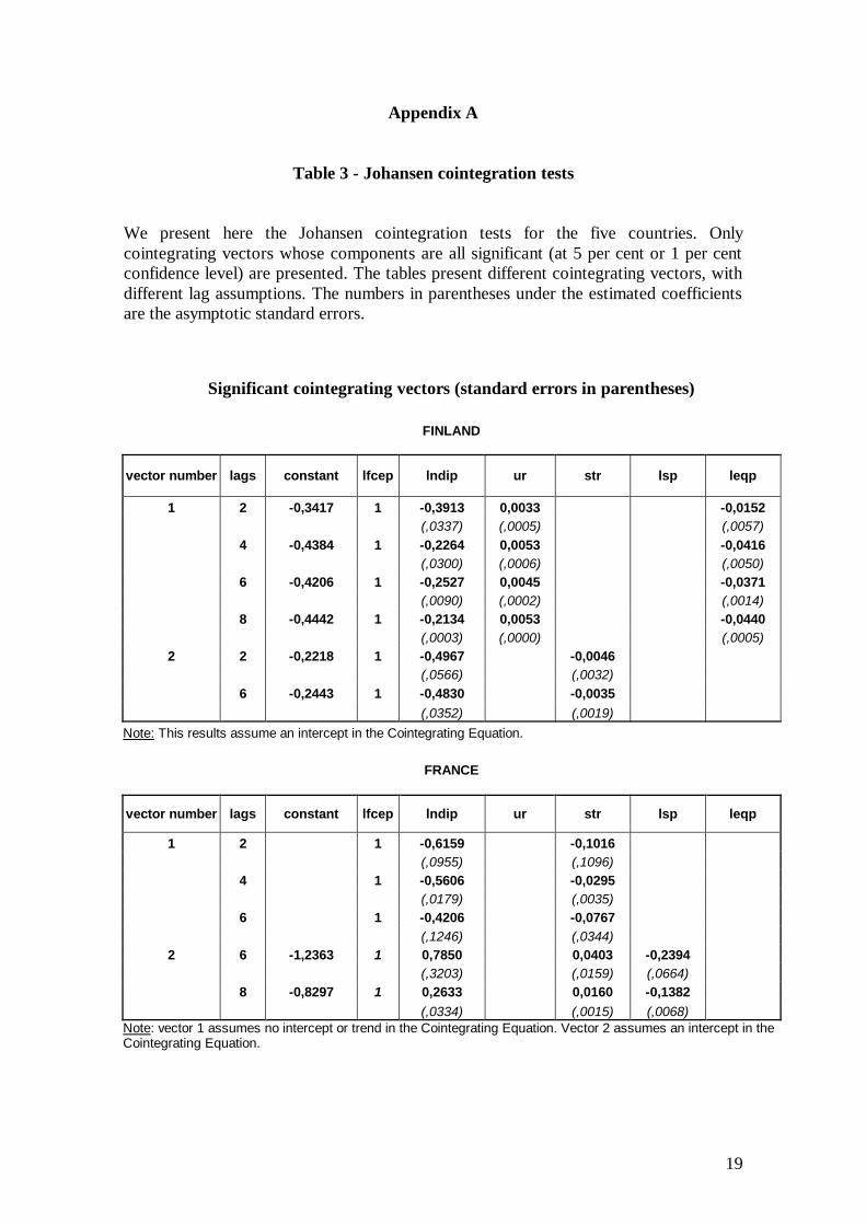
Table 3 - Johansen cointegration tests We present here the Johansen cointegration tests for the five countries. Only cointegrating vectors whose components are all significant (at 5 per cent or 1 per cent confidence level) are presented. The tables present different cointegrating vectors, with different lag assumptions. The numbers in parentheses under the estimated coefficients are the asymptotic standard errors.
Significant cointegrating vectors (standard errors in parentheses)
FINLAND
vector number lags constant lfcep lndip ur str lsp leqp
1 2 -0,3417 1 -0,3913 0,0033 -0,0152 (,0337) (,0005) (,0057) 4 -0,4384 1 -0,2264 0,0053 -0,0416 (,0300) (,0006) (,0050) 6 -0,4206 1 -0,2527 0,0045 -0,0371 (,0090) (,0002) (,0014) 8 -0,4442 1 -0,2134 0,0053 -0,0440 (,0003) (,0000) (,0005) 2 2 -0,2218 1 -0,4967 -0,0046 (,0566) (,0032) 6 -0,2443 1 -0,4830 -0,0035 (,0352) (,0019)
Note: This results assume an intercept in the Cointegrating Equation.
FRANCE
vector number lags constant lfcep lndip ur str lsp leqp
1 2 1 -0,6159 -0,1016 (,0955) (,1096) 4 1 -0,5606 -0,0295 (,0179) (,0035) 6 1 -0,4206 -0,0767 (,1246) (,0344) 2 6 -1,2363 1 0,7850 0,0403 -0,2394 (,3203) (,0159) (,0664) 8 -0,8297 1 0,2633 0,0160 -0,1382 (,0334) (,0015) (,0068)
Note: vector 1 assumes no intercept or trend in the Cointegrating Equation. Vector 2 assumes an intercept in the Cointegrating Equation.

20
Table 3 (cont.)
GERMANY
vector number lags constant lfcep lndip ur str lsp leqp
1 4 1 -0,0151 -0,2219 (,0076) (,0137) 6 1 0,0044 -0,2082 (,0039) (,0046) 8 1 0,0084 -0,2117 (,0025) (,0036) 2 2 0,0055 1 -0,6840 -0,0236 (,1078) (,0060) 6 -0,1948 1 -0,5791 -0,0164 (,0207) (,0010) 8 -0,0933 1 -0,6575 -0,0118 (,0386) (,0022)
Note: vector 1 assumes no intercept or trend in the Cointegrating Equation. Vector 2 assumes an intercept in the Cointegrating Equation.
PORTUGAL
vector number lags constant lfcep lndip ur str lsp leqp
1 4 0,27542 1 -0,5655 -0,0352 (,0344) (,0064) 2 2 -0,2470 1 -0,3121 0,0242 (,0517) (,0041) 4 -0,0287 1 -0,2656 0,0245 (,0197) (,0013)
Note: This results assume an intercept in the Cointegrating Equation.
UNITED KINGDOM
vector number lags constant lfcep lndip ur str lsp leqp
lrep
1 6 -0,7218 1 0,0466 -0,0873 (,0094) (,0304) 2 4 -0,2659 1 0,3692 0,0595 -0,2732 (,1495) (,0134) (,0624) 6 -0,1828 1 0,1984 0,0406 -0,2216 (,0770) (,0054) (,0366) 8 -0,4901 1 0,1864 0,0518 -0,1797 (,0680) (,0060) (,0365)
Note: This results assume an intercept in the Cointegrating Equation.

21
Appendix B
Description of variables
Variable
Unit
Designation Country sample
Final consumption expenditure by
households (per capita)
Millions of euros
(1995 prices)
fcep Finland: 80:1-01:4 France: 80:1-01:4 Germany: 91:1-01:4 Portugal: 95:1-01:3 United Kingdom: 80:1-01:3
Net disposable income (per capita) Millions of euros
(1995 prices)
ndip Finland: 80:1-01:4 France: 80:1-01:4 Germany: 91:1-01:4 Portugal: 95:1-01:3 United Kingdom: 80:1-01:3
Short-term interest rate (3M) Percentage str Finland: 80:1-01:4 France: 80:1-01:4 Germany: 91:1-01:4 Portugal: 95:1-01:3 United Kingdom: 80:1-01:3
Harmonized unemployment rate Percentage ur Finland: 89:1-01:4 France: 83:1-01:4 Germany: 91:1-01:4 Portugal: 95:1-01:3 United Kingdom: 83:1-01:3
Share prices index Index (1995 = 100) sp Finland: 91:1-01:4 France: 87:4-01:4 Germany: 91:1-01:4 Portugal: 95:1-01:3 United Kingdom: 90:1-01:3
Equities prices index Index (1985 = 100) eqp Finland: 80:1-01:4 France: 80:1-01:4 Germany: 91:1-01:4 United Kingdom: 80:1-01:3
Residential prices index Index (1985 = 100) rep Finland: 80:1-01:4 United Kingdom: 80:1-01:3
Where logs were applied the variable appears with the letter l and when in first differences it appears with the letter d.
Top Related