


![Computer Animation - Princeton University Computer … · Pixar 3-D and 2-D animation Homer 3-D Homer 2-D ... Disney Computer Animation Animation pipeline ... 18-animation.ppt [Read-Only]](https://static.fdocuments.in/doc/165x107/5b40ec327f8b9a4b3f8db714/computer-animation-princeton-university-computer-pixar-3-d-and-2-d-animation.jpg)


Languages
Pages
Legal

Artificial Animalsfor Computer Animation:
Biomechanics, Locomotion, Perception, and Behavior
by
Xiaoyuan Tu
A thesis submitted in conformity with the requirementsfor the degree of Doctor of Philosophy
Graduate Department of Computer ScienceUniversity of Toronto
c�
Copyright by Xiaoyuan Tu 1996

c�
Xiaoyuan Tu 1996
ALL RIGHTS RESERVED
Artificial Animals for Computer Animation:Biomechanics, Locomotion, Perception, and Behavior
Doctor of Philosophy, 1996
Xiaoyuan Tu
Department of Computer Science, University of Toronto
Abstract
This thesis develops an artificial life paradigm for computer graphics animation. Animals in theirnatural habitats have presented a long-standing and difficult challenge to animators. We proposea framework for achieving the intricacy of animal motion and behavior evident in certain naturalecosystems, with minimal animator intervention.
Our approach is to construct artificial animals. We create self-animating, autonomous agentswhich emulate the realistic appearance, movement, and behavior of individual animals, as well asthe patterns of social behavior evident in groups of animals. Our computational models achievethis by capturing the essential characteristics common to all biological creatures—biomechanics,locomotion, perception, and behavior.
To validate our framework, we have implemented a virtual marine world inhabited by a variety ofrealistic artificial fishes. Each artificial fish is a functional autonomous agent. It has a physics-based,deformable body actuated by internal muscles, sensors such as eyes, and a brain with perception,motor, and behavior control centers. It swims hydrodynamically in simulated water through thecontrolled coordination of its muscle actions. Artificial fishes exhibit a repertoire of behaviors.They explore their habitat in search of food, navigate around obstacles, contend with predators, andindulge in courtship rituals to secure mates. Like their natural counterparts, their behavior is basedon their perception of the dynamic environment and their internal motivations.
Since the behavior of artificial fishes is adaptive to their virtual habitat, their detailed motionsneed not be keyframed nor scripted. This thesis therefore demonstrates a powerful approach tocomputer animation in which the animator plays the role of a nature cinematographer, rather thanthe more conventional role of a graphical model puppeteer. Our work not only achieves behavioralanimation of unprecedented complexity, but it also provides an interesting experimental domain forrelated research disciplines in which functional, artificial animals can serve as autonomous virtualrobots.
i
Acknowledgment
First, I would like to thank my advisors Demetri Terzopoulos and Eugene Fiume. This thesis
would not have been possible without their support.
Demetri has been my mentor in the exciting fields of computer animation and physics-based
graphics modeling. His many remarkable qualities have benefited me greatly. I am most impressed
by his breadth of knowledge,his ability to seize new ideas,his openmindedness, and his perfectionism
towards technical writing. I am especially grateful for the unfailing encouragement he has given me
through the years. I would not have come this far this quickly without his expert guidance and the
substantial time and effort he has put into my thesis.
I thank Eugene for giving me the chance to join the graphics group three years ago. Without
his kindness, I would have been stuck studying boring operating systems (no offense intended). I
appreciate his many insightful comments that have helped to improve my thesis and to put my view
into perspective.
My special thanks go to Professor Daniel Thalmann for generously agreeing to serve as external
examiner of my thesis, despite his busy schedule and the long distance he had to travel. Special
thanks also go to Professor Janet Halperin for serving as internal examiner and Professor Michiel
Van de Panne for serving as internal appraiser on my thesis committee. Many thanks to Professors
Ken Sevcik and Geoffrey Hinton for serving on my committee and providing valuable comments on
my thesis.
I thank the wonderful people of the graphics and vision labs. My years at U of T would have been
dull without them. I would like to express my sincere gratitude to Tamara Stephas, Meng Sun, Victor
Ng, Xiaohuan Wang, Petros Faloutsos, Jeremy Cooperstock, Radek Grzeszczuk, Beverly Harrison,
Kevin Schlueter, Michael McCool, Alex Mitchell, Jeff Tupper, Jos Stam, Sherif Ghali, Joe Laszlo,
William Hunt and Baining Guo from the graphics lab, and Tim McInerney, Victor Lee and Xuan
Ju from the vision lab. My deep appreciation to my friends from other groups in the department,
Vincent Gogan, Steven Shapiro and Michalis Faloutsos, and, from elsewhere, Yuxiang Wang, Wei
Xu, Tina Shapiro and Christopher Lori. Particularly, I thank my colleague Radek Grzeszczuk, for
ii
collaborating in the production of “Cousto”. Thanks also to Kathy Yen for helping me to deal with
the many tedious details in arranging my defense.
I would especially like to thank Michiel Van de Panne, who was a student at the graphics lab
when I started my PhD program and now, as I finish, is a professor. He has always been very
generous in helping others around the lab. He taught me how to use the video equipment and
provided substantial assistance in the production of my animations.
I thank my parents, to whom I dedicate this thesis, for their endless love and support, for their
unwavering confidence in me and their limitless patience. They are the best parents I could have
ever dreamed to have.
Finally, thanks to my partner John, for his love, support, help (both as a colleague and a friend)
and the wonderful times he brings me.
iii

iv
Contents
1 Introduction 1
1.1 Motivation ������������������������������������������������������������������������� 1
1.2 Challenges ������������������������������������������������������������������������� 2
1.2.1 Conventional Animation Techniques ��������������������������������������� 3
1.3 Methodology: Artificial Life for Computer Animation ����������������������������� 5
1.3.1 Criteria and Goals ��������������������������������������������������������� 5
1.3.2 Artificial Animals ��������������������������������������������������������� 5
1.3.3 From Physics to Realistic Locomotion ������������������������������������� 6
1.3.4 Realistic Perception ������������������������������������������������������� 8
1.3.5 Realistic Behavior ��������������������������������������������������������� 8
1.3.6 Fidelity and Efficiency ����������������������������������������������������� 9
1.4 Contributions and Results ��������������������������������������������������������� 10
1.4.1 Primary Contributions ����������������������������������������������������� 11
1.4.2 Auxiliary Technical Contributions ����������������������������������������� 14
1.5 Thesis Overview ������������������������������������������������������������������� 15
2 Background 17
2.1 Physics-Based Modeling ����������������������������������������������������������� 17
2.1.1 Constraint-based Approach ����������������������������������������������� 18
2.1.2 Motion Synthesis Approach ����������������������������������������������� 19
2.2 Behavioral Animation ������������������������������������������������������������� 22
v
2.2.1 Perception Modeling ������������������������������������������������������� 23
2.2.2 Control of Behavior ������������������������������������������������������� 24
2.3 The Modeling of Action Selection ������������������������������������������������� 25
2.3.1 Defining Action ����������������������������������������������������������� 25
2.3.2 Goals and Means ����������������������������������������������������������� 27
2.3.3 Previous Work ������������������������������������������������������������� 28
2.3.4 Task-level Motion Planning ����������������������������������������������� 30
2.4 Summary ��������������������������������������������������������������������������� 30
3 Functional Anatomy of an Artificial Fish 33
3.1 Motor System ��������������������������������������������������������������������� 35
3.2 Perception System ����������������������������������������������������������������� 35
3.3 Behavior System ������������������������������������������������������������������� 35
4 Biomechanical Fish Model and Locomotion 37
4.1 Discrete Physics-Based Models ��������������������������������������������������� 37
4.2 Structure of the Dynamic Fish Model ��������������������������������������������� 38
4.3 Mechanics ������������������������������������������������������������������������� 41
4.3.1 Viscoelastic Units ��������������������������������������������������������� 41
4.4 Muscles and Hydrodynamics ������������������������������������������������������� 44
4.5 Numerical Solution ����������������������������������������������������������������� 46
4.5.1 System Matrix Assembling and the Skyline Storage Scheme ������������� 48
4.5.2 Algorithm Outline and Discussion ����������������������������������������� 51
4.6 Motor Controllers ����������������������������������������������������������������� 52
4.6.1 Muscle Motor Controllers ������������������������������������������������� 53
4.6.2 Pectoral Fin Motor Controllers ��������������������������������������������� 57
5 Modeling the Form and Appearance of Fishes 59
5.1 Constructing 3D Geometric Fish Models ������������������������������������������� 59
vi
5.2 Obtaining Texture Coordinates ����������������������������������������������������� 62
5.2.1 Deformable Mesh ��������������������������������������������������������� 63
5.3 Texture-Mapped Models ����������������������������������������������������������� 64
5.4 Coupling the Dynamic and Display Models ��������������������������������������� 65
5.5 Visualization of the Pectoral Motions ��������������������������������������������� 67
6 Perception Modeling 71
6.1 Perception Modeling for Animation ����������������������������������������������� 71
6.2 Overview of the Artificial Fish’s Perception System ������������������������������� 73
6.3 Vision Sensor Modeling ����������������������������������������������������������� 73
6.3.1 Perceptual Range ��������������������������������������������������������� 74
6.3.2 Occlusion ����������������������������������������������������������������� 75
6.3.3 Functionality ��������������������������������������������������������������� 75
6.4 Computing Visibility ��������������������������������������������������������������� 77
6.4.1 Visibility of a Point ������������������������������������������������������� 77
6.4.2 Visibility of Another Fish ������������������������������������������������� 80
6.4.3 Visibility of a Cylinder ����������������������������������������������������� 80
6.4.4 Visibility of Seaweeds ����������������������������������������������������� 80
6.4.5 Discussion ����������������������������������������������������������������� 81
6.5 The Focusser ����������������������������������������������������������������������� 82
6.5.1 Focus of Attention in Animals ��������������������������������������������� 82
6.5.2 Design of the Focusser ����������������������������������������������������� 83
6.5.3 Summary ����������������������������������������������������������������� 86
6.6 From Perception to Behavior ������������������������������������������������������� 87
6.6.1 An Example: Collision Detection ����������������������������������������� 87
6.7 Synthetic Vision Models ����������������������������������������������������������� 90
7 The Behavior System 93
vii
7.1 Effective Action Selection Mechanisms ������������������������������������������� 94
7.2 Behavior Control and Ethology ��������������������������������������������������� 95
7.2.1 The Intention Level ������������������������������������������������������� 95
7.2.2 The Action Level ��������������������������������������������������������� 95
7.2.3 Summary ����������������������������������������������������������������� 97
7.3 Habits ����������������������������������������������������������������������������� 98
7.4 Mental State ����������������������������������������������������������������������� 98
7.5 Intention Generator ����������������������������������������������������������������� 101
7.5.1 Why Hierarchy? ����������������������������������������������������������� 103
7.6 Intention-Guided Perception: Control of the Focusser ����������������������������� 104
7.7 Persistence in Behavior ����������������������������������������������������������� 105
7.7.1 Behavior Memory ��������������������������������������������������������� 105
7.7.2 Inhibitory Gain and Fatigue ����������������������������������������������� 106
7.7.3 Persistence in Targeting ��������������������������������������������������� 106
7.8 Behavior Routines ����������������������������������������������������������������� 107
7.8.1 Primitive Behavior: Avoiding Potential Collisions ������������������������� 108
7.8.2 Primitive Behavior: Moving Target Pursuit ������������������������������� 108
7.9 Artificial Fish Types ��������������������������������������������������������������� 112
7.9.1 Predators ������������������������������������������������������������������� 112
7.9.2 Prey ����������������������������������������������������������������������� 114
7.9.3 Pacifists ������������������������������������������������������������������� 119
7.10 Discussion ������������������������������������������������������������������������� 124
7.10.1 Analysis ������������������������������������������������������������������� 124
7.10.2 Summary ����������������������������������������������������������������� 126
8 Modeling the Marine Environment 129
8.1 Water Current ��������������������������������������������������������������������� 129
8.2 Seaweeds and Plankton ����������������������������������������������������������� 130
viii
9 The Graphical User Interface 133
9.1 Initialization Panels ��������������������������������������������������������������� 133
9.2 Manipulation Panels ��������������������������������������������������������������� 134
9.3 Control Panels ��������������������������������������������������������������������� 137
9.4 Discussion ������������������������������������������������������������������������� 138
10 Animation Results 141
10.1 “Go Fish!” ������������������������������������������������������������������������� 141
10.2 “The Undersea World of Jack Cousto” ��������������������������������������������� 144
10.3 Animation Short: Preying Behavior ����������������������������������������������� 144
10.4 Animation Short: Schooling Behavior ��������������������������������������������� 146
10.5 Animation Short: Mating Behavior ����������������������������������������������� 147
11 Conclusion and Future Work 149
11.1 Conclusion ������������������������������������������������������������������������� 149
11.2 Additional Impact in Animation and Artificial Life ������������������������������� 150
11.3 Impact in Computer Vision and Robotics ������������������������������������������� 152
11.4 Potential Applications in Ethology ������������������������������������������������� 153
11.5 Other Artificial Animals ����������������������������������������������������������� 154
11.6 Future Research Directions ��������������������������������������������������������� 155
11.6.1 Animation ����������������������������������������������������������������� 155
11.6.2 Artificial Life ������������������������������������������������������������� 157
A Deformable Contour Models 158
B Visualization of the Pectoral Motions 161
B.1 Animating the Pectoral Flapping Motion ������������������������������������������� 161
B.2 Animating the Pectoral Oaring Motion ��������������������������������������������� 163
C Prior Action Selection Mechanisms 164
ix

C.1 Behavior Choice Network ��������������������������������������������������������� 164
C.2 Free-Flow Hierarchy ��������������������������������������������������������������� 165
D Color Images 173
x
List of Figures
1.1 Artificial fishes in their physics-based world. See the original color image in Appendix D . 12
1.2 Mating behavior. Female (top) is courted by larger male. See the original color imagein Appendix D . ��������������������������������������������������������������������� 12
1.3 Predator shark stalking school of prey fish. See the original color image in Appendix D . 13
2.1 Differentiating action selection from motor control in design. ��������������������� 26
3.1 System overview of the artificial fish. ��������������������������������������������� 34
4.1 The motor system of an artificial fish. ��������������������������������������������� 38
4.2 The biomechanical fish model. ����������������������������������������������������� 40
4.3 The top and side view of the outline of the fish model at rest. ��������������������� 40
4.4 Uniaxial elastic, viscous, and viscoelastic units. ����������������������������������� 42
4.5 Hydrodynamic locomotion. ������������������������������������������������������� 45
4.6 Structure of the system matrix. ����������������������������������������������������� 49
4.7 The skyline storage scheme. ������������������������������������������������������� 50
4.8 Top view of an artificial fish during caudal swimming motion. ��������������������� 55
4.9 Photograph of real fish swimming. ������������������������������������������������� 55
4.10 Top-front view of an artificial fish during caudal swimming motion. ��������������� 55
4.11 The steering map. ����������������������������������������������������������������� 56
4.12 The turning motion of the artificial fish. ������������������������������������������� 56
4.13 The pectoral fin geometry. ��������������������������������������������������������� 57
4.14 The local coordinate system of a fish. ��������������������������������������������� 58
xi
5.1 Digital images of real fish. ��������������������������������������������������������� 60
5.2 Control-point mesh of the left half of a fish body. ��������������������������������� 61
5.3 The shaded NURBS surface of the left half of a fish body. ��������������������������� 61
5.4 Geometric model of fish body with fins. ������������������������������������������� 62
5.5 Control-point mesh fish models. ��������������������������������������������������� 62
5.6 Initial and stabilized deformable mesh. ��������������������������������������������� 64
5.7 Texture mapped 3D fish models. ��������������������������������������������������� 64
5.8 The subdivision of the faces of the dynamic fish. ����������������������������������� 66
5.9 Geometric mesh surface overlayed on dynamic fish model. ����������������������� 68
5.10 The geometric NURBS surface fish deforms with the dynamic fish. ����������������� 68
5.11 Snapshots of the pectoral flapping motion. ����������������������������������������� 69
5.12 Snapshots of the pectoral oaring motion of a butterfly fish. ������������������������� 69
6.1 The perception system in an artificial fish. ����������������������������������������� 73
6.2 Vision sensor. ��������������������������������������������������������������������� 74
6.3 Occlusion and distance limit visual perception. ����������������������������������� 75
6.4 Fisheye view of the world showing fishing line. See the original color image in AppendixD . ��������������������������������������������������������������������������������� 76
6.5 Fisheye view of the world showing hooked fish. ����������������������������������� 77
6.6 Occlusion test. ��������������������������������������������������������������������� 78
6.7 Swimming fishes avoiding collisions with cylindrical obstacles. ������������������� 88
6.8 The fish’s collision sensitivity region. ��������������������������������������������� 90
6.9 Analogues of intrinsic images. ����������������������������������������������������� 92
7.1 The behavior system in an artificial fish. ������������������������������������������� 94
7.2 The control scheme for action selection. ������������������������������������������� 96
7.3 The form of the stimulus functions ������ and ������� . ������������������������������� 100
7.4 Generic intention generator. ������������������������������������������������������� 102
7.5 Outline of chasing-target routine. ������������������������������������������������� 109
xii
7.6 The position of target relative to fish. ����������������������������������������������� 109
7.7 A peaceful marine world. See the original color image in Appendix D . ��������������� 111
7.8 The smell of danger. See the original color image in Appendix D . ������������������� 111
7.9 The intention generator of a predator. ��������������������������������������������� 112
7.10 The angle ��� . ��������������������������������������������������������������������� 113
7.11 A hungry predator ingesting prey. ������������������������������������������������� 114
7.12 Portion of intention generator of prey. ��������������������������������������������� 114
7.13 Schooling behavior routine. ������������������������������������������������������� 115
7.14 A small school of angelfish. ������������������������������������������������������� 116
7.15 An inceptive school. ��������������������������������������������������������������� 116
7.16 A school of fish encounters an obstacle. ������������������������������������������� 117
7.17 School scatters in terror. ����������������������������������������������������������� 118
7.18 Fleeing from predator. ������������������������������������������������������������� 118
7.19 Mating behaviors in real fishes. ��������������������������������������������������� 121
7.20 Two males (larger) vying for the attention of a female. ����������������������������� 122
7.21 A clownfish displays opportunism in behavior. ������������������������������������� 126
8.1 The flow primitives. ��������������������������������������������������������������� 129
8.2 The swaying motion of a seaweed in simulated water currents. ��������������������� 131
8.3 The seaweed responds to hydrodynamic forces produced by a passing fish. ������� 132
9.1 The object initialization panel. ����������������������������������������������������� 134
9.2 The position initialization panel. ��������������������������������������������������� 135
9.3 The physical parameter panel. ����������������������������������������������������� 135
9.4 The behavior panel. ��������������������������������������������������������������� 136
9.5 The habit panel. ������������������������������������������������������������������� 137
9.6 The general control panel. ��������������������������������������������������������� 138
9.7 The fishview control panel and the rendered identity maps from fish ‘1’. ����������� 139
xiii
10.1 Denizens of the virtual marine world happily feeding on plankton. ����������������� 142
10.2 Hungry fishes approaching the hook. ����������������������������������������������� 143
10.3 A hapless fish is caught and pulled to the surface. ��������������������������������� 143
10.4 A dangerous shark stalking a school of prey. ��������������������������������������� 145
10.5 A school of fleeing prey. ����������������������������������������������������������� 145
10.6 A pair of courting pokerfish. ������������������������������������������������������� 146
10.7 A large predator hunting small prey fishes while pacifist fishes, untroubled by thepredator, feed on plankton. ��������������������������������������������������������� 147
11.1 Locomotion learning center in the brain of the artificial fish. ����������������������� 151
B.1 Visualization of pectoral fin motion. ����������������������������������������������� 162
xiv
Chapter 1
Introduction
A kangaroo hops across a barren plain. It leaps and lands rhythmically. The harmonic movements
of its body, legs and tail trace out graceful curves in the air. A flock of birds glides across the sky.
Individual birds flap their wings and adjust their direction autonomously, yet they all fly in unison.
1.1 Motivation
Animals in motion have intrigued computer graphics animators and researchers for several decades.
They have long been the subject of study of zoologists and ethologists, and have recently helped
inspire the emerging research discipline of artificial life.
In computer graphics, most animations of animals have been created using the traditional and
often highly labour intensive keyframing technique, in which computers are employed to interpolate
between animator-specified keyframes (Lasseter, 1987). More recently, increasingly automated
techniques for synthesizing realistic animal motion have drawn much attention. Successful attempts
have been made to animate the motions of humans (Magnenat-Thalmann and Thalmann, 1990;
Hodgins, Sweeney and Lawrence, 1992), of certain animals (Miller, 1988; Girard, 1991) and of
some imaginary creatures (Witkin and Kass, 1988; van de Panne and Fiume, 1993; Ngo and Marks,
1993). However, motion synthesis is only part of the challenge of animating animals. Some group
behaviors evident in the animal world, such as flocking, schooling and herding (Reynolds, 1987)
have also been simulated and realistically animated in recent feature films.
In this dissertation, we will investigate the problem of producing animation which captures
1
2 CHAPTER 1. INTRODUCTION
the intricacy of motion and behavior evident in certain natural ecosystems. These animations are
intrinsically complex and present a challenge to the computer graphics practitioner. Animations
of this sort are of interest not only because they attempt to recreate fascinating natural scenarios,
but also because they have broad applicability. They can be used in the entertainment industry, for
special effects in movies, for video games, for virtual reality rides; as well as in education as, say,
interactive educational tools for teaching biology.
Our goal will be to create the animations that we have described, not by conventional keyframing,
but rather through the sophisticated modeling of animals and their habitats. To this end, we have
been motivated by and have contributed to the artificial life (ALife) movement (Levy, 1992). ALife
complements the traditional analytic approach of biology by aiming to understand natural life
through synthetic, computational means. That is to say, rather than studying biological phenomena
by analyzing living systems, the ALife approach attempts to synthesize artificial systems that behave
like living organisms. An important area of ALife research is the synthesis of artificial animals—or
“animats”—implemented both in software and in hardware (Meyer and Guillot, 1991; Cliff et al.,
1994). Computational models of simple animals, such as single-cell life forms (Langton, 1987) and
insects (Beer, 1990), have been proposed with interesting results. Many of these models draw upon
theories of animal behavior put forward by ethologists (Manning, 1979; McFarland, 1971).
Since we will view the animation of natural ecosystems as the process of visualizing computer
simulations of animals in their habitats, our work straddles the boundary between the fields of
computer graphics and artificial life. This theme has also been investigated by Terzopoulos et al.
(1995).
1.2 Challenges
Natural ecosystems are as challenging to animate as they are fascinating to watch. The major
challenge comes from their intrinsic complexity. In a given animation system, there may be a large
number of animals, each of which may exhibit elaborate behaviors. Ideally, one would like to achieve
an abundance of natural intricacy with minimal effort on the part of the animator. The challenge
is exacerbated when one also demands visual authenticity in the appearance and locomotion of
individual animals and in their behavior.
Ecosystems are characterized by the relationships between animals and their habitats. This means
that when we look at an ecosystem, we are keenly aware of the behaviors exhibited by animals as
1.2. CHALLENGES 3
they interact with their dynamic environment, especially with other animals. For example, a hunting
scenario will not seem authentic if a rabbit hops around carelessly disregarding the presence of
a hungry wolf, or if a crowd of pigeons rest calmly while a child runs in their midst. People’s
familiarity with various animals imposes strict criteria for the evaluation of the visual results of our
proposed simulations, since even small imperfections in the animated motions or behaviors will be
readily recognizable.
Visual realism, however, is not the only constraint on such animations. For applications in the
entertainment and educational industries, the animator should be able to control various aspects of
an animation. It is especially important to be able to easily modify an animation; for example,
altering the virtual environment, changing the number, types and distribution of the virtual animals
and, moreover, varying the personalities of the animals and even interacting with them.
1.2.1 Conventional Animation Techniques
Traditional computer animation techniques, such as keyframing, have been used to create many
great animations, including those of animals. However, they have several limitations:
Significant Animator Intervention is Required
Perhaps the most spectacular instance to date of conventional animation techniques applied to the
animation of animals is the dinosaurs in the blockbuster feature film “Jurassic Park” (a 1993 Amblin
Entertainment Production for Universal Pictures). Yet as realistic looking as they may be, these
dinosaurs are merely graphical puppets which require teams of highly skilled human animators to
plot their actions and detailed motions carefully from one step to the next. This reveals the main
drawback of keyframing: The amount of effort expended by the animator increases dramatically
with the length, complexity and intended realism of the animation.
Techniques that do not require as much animator skill, such as motion capture schemes (Calvert,
Chapman and Patla, 1980), have also been widely used in producing realistic animated motions.
However, they tend to be inflexible, since they produce motions that are highly specific, hard to
parameterize, and difficult to compose into lengthier animations. Moreover, such schemes are not
easily applied to non-human or imaginary creatures.
4 CHAPTER 1. INTRODUCTION
Characters Lack Autonomy
The lack of autonomy of keyframed or motion-data driven characters detracts from the modifiability
and interactability of the animation. Since realistic behaviors of an animal are subject to the state
of its environment (which contains immobile and mobile objects, such as trees, stones, and other
animals), slight modifications in a scripted animation, such as moving a tree or adding another
animal, may require that the entire animation be re-scripted. Graphical puppets are incapable of
actively interacting with their environment. As a result, keyframing techniques are ill-suited to
applications such as virtual reality, computer games and interactive educational tools.
Low-Level Motion Specification is Burdensome
Using conventional animation techniques, animations are specified at a very low level, thus granting
the animator complete control over every aspect of the animation. Complete animator control is
sometimes required, especially in cartooning; however, it is generally unnecessary for the sorts of
applications in which we are interested. Consider the case of animating a realistic virtual zoo: It
is not important if some particular animal appears in some specific posture at some specific time
instant; what is important is for the lions and monkeys to look real and for them to move and behave
realistically. Complete animator control is also undesirable in our case because it implies little or
no autonomy in the animated characters themselves. Therefore, a good strategy for our purposes is
to relinquish low-level animator control in favor of a much higher level of control.
Physical Realism is Not Guaranteed
Last but not least, using conventional keyframing techniques, realism depends solely upon the skills
of the animator. Unless the animator is highly skilled, poor visual results may obtain. In particular,
since conventional geometric models possess no mechanical properties, the physical correctness of
the resulting motion is not guaranteed, nor will the animated figures respond to forces in a realistic
manner.
1.3. METHODOLOGY: ARTIFICIAL LIFE FOR COMPUTER ANIMATION 5
1.3 Methodology: Artificial Life for Computer Animation
1.3.1 Criteria and Goals
In light of the preceding discussion, we seek an approach to animating natural ecosystems that is
capable of achieving realistic visual effects through an automatic process. The desired properties of
such an approach are as follows:
1. The appearance, locomotion and behavior of the animated creatures should be visually con-
vincing.
2. The creatures should have a high degree of autonomy so that this can be achieved with minimal
animator intervention. The level of autonomy in the animated animals should, however, permit
and support the necessary degree of high-level animator control:
� The animator should be able to alter the initial conditions of the animation, such as the
number and positions of immobile and mobile objects in the virtual habitat.
� The animator should be able to influence or direct the behaviors of the animated charac-
ters to some degree.
The research reported in this thesis develops a highly automatic approach to creating life-like
animations and validates it through implementation. Realism is achieved through advanced modeling
of animals and their habitats.
1.3.2 Artificial Animals
We believe that the best way of achieving our goals in the long run is to pursue the challenging
approach of constructing artificial animals. The properties and internal control mechanisms of
artificial animals should be qualitatively similar to those of their natural counterparts.
There are several properties common to all animals. The most salient one is that all animals are
autonomous: They have physical bodies that are actuated by muscles, enabling them to locomote;
they have eyes and other sensors to actively perceive their environment; they have brains which
interpret their perceptions and govern their actions. Indeed, autonomy is the consequence of
possessing a brain capable of controlling perception and action in a physical body. The behavior of
6 CHAPTER 1. INTRODUCTION
an animal is a consequence of its autonomous interaction with its environment to satisfy its survival
needs. No external control is required for animals to cope with their dynamic habitats, yet their
autonomy does not prevent higher animals from being influenced or directed (consider trained circus
animals, or human actors).
Artificial animals should be self-animating actors that emulate the autonomy of real animals. In
our artificial life approach to computer animation, we build animal-like autonomy into our graphics
models; not only to minimize the amount of animator intervention while supporting modifiability
and interactability, but also to obtain behavioral realism. Our main concern is how to model the
locomotion, perception and behavior capabilities of animals and how to integrate these models
effectively within a life-like artificial animal. Our research in this respect shares common goals with
ALife research, where artificial animals are often referred to as “animats”. Previous animats have
been models of simple creatures and the behaviors simulated usually pertain to genetic reproduction
and “natural selection” (Langton, 1987; Varela and Bourgine, 1991). We attempt to develop artificial
life patterned after animals that are more evolved and have a significantly broader range of behavior.
In the following sections, we will identify the essential properties and mechanisms that allow
real animals to locomote effectively, to perceive, and hence to behave autonomously. From this we
derive design methodologies for achieving realistic animated locomotion and behavior with minimal
animator intervention.
1.3.3 From Physics to Realistic Locomotion
Physics-Based Modeling
The motion of any physical entity is governed at the lowest level by the laws of physics. The use
of physics is not new to computer graphics. It was introduced as “physics-based modeling” about
a decade ago (Armstrong and Green, 1985; Wilhelms, 1987; Terzopoulos et al., 1987) and has
spawned a large body of advanced graphics modeling and animation research. Using physics-based
models for graphics not only ensures physical realism of the resulting motion, it also allows subtle
yet visually important motions to be animated automatically. Consider, for example, the realistic
animation of a stampeding elephant. It would be a heroic chore to try to apply manual keyframing
or other purely kinematic methods to animate the rippling flesh, the flapping ears, or the swinging
trunk and tail. Physics-based modeling is capable of producing such motions automatically. More
details about physics-based modeling and related previous work can be found in Chapter 2.
1.3. METHODOLOGY: ARTIFICIAL LIFE FOR COMPUTER ANIMATION 7
Simulated Physical Body
The laws of physics and the principles of biomechanics shape the appearance of animal motion.
Therefore, the best way to achieve realistic locomotion is to simulate their effects. According to
mechanics, the change of the state of an object, or what we commonly call “movement”, is caused
by forces. The motion of an inanimate object, such as a stone, is generally caused by unbalanced
external forces and hence is passive. The motion of an animal, on the other hand, is generally
initiated by unbalanced internal forces actively generated by its muscles and hence is active. Each
species of animal has its particular body structure and arrangement of muscles. This in turn dictates
its particular mode of locomotion. We therefore construct simulated physical bodies for our artificial
animals. By doing so, the laws of physics will guarantee the physical correctness of the resulting
motion, while the biomechanical principles relevant to the animal of interest can yield natural muscle
actions that simulate the particular locomotion patterns characteristic of the animal in its physical
environment.
Simulated Physical Environment
The locomotion of an animal not only derives from the dynamics of its body but also is a result of
the dynamics of its environment. In accordance with biomechanical principles, various locomotion
patterns of animals—e.g. flying, swimming or running—emerge from the interaction between their
active muscle-actuated body movements and the reactive physical environment—air, water, or terra
firma. For example, birds flap their wings inducing aerodynamic forces, which in turn enable them
to fly through the air. They cannot fly in a vacuum. Therefore, in addition to modeling the physics
of animal bodies, we need also to model the physics of their environments.
Motor Control
Upon the computational physics substrate, computed via a dynamic simulation, it is possible to
generate realistic locomotion of the artificial animal through simulated muscle control. Through
evolution, most natural animals have developed their particular mechanisms for motor control, where
coordinated muscle activations result in energy-efficient locomotion. Effective motor controllers
can be derived based on the a priori knowledge about the characteristic muscle activations of the
corresponding real animal.
8 CHAPTER 1. INTRODUCTION
1.3.4 Realistic Perception
In order to survive in dynamic and often hostile environments, animals are able to adapt their
behaviors according to the current situation. As summarized by the ethologist Manning (1979), the
behavior of an animal “includes all those processes by which the animal senses the external world and
the internal state of its body and responds to changes which it perceives.” This definition emphasizes
the crucial dependence of animal behavior on perception, for without perception, an animal cannot
possibly react to its environment. To increase their chances of survival, most animals have evolved
acute perceptual modalities, especially eyes, to detect opportunities and dangers in their habitat. The
sense organs of animals have specific capabilities and inherent limitations. For example vision is
most effective within some proximal distance because, under most circumstances, spatially proximal
events will have the greatest effect on an animal. Furthermore, vision is not possible through opaque
objects. We must model both the capabilities and the limitations of perception correctly for our
artificial animals to exhibit realistic behavior.
1.3.5 Realistic Behavior
Given that an animal has the ability to locomote and to sense its environment, its brain is able to
interpret the sensory information and select appropriate actions to yield a useful range of behavior.
Environment, External Stimuli and Internal State
To enable an artificial animal to behave realistically and autonomously, it is necessary to model
relevant aspects of its habitat as well as its internal mental state. Sensory stimuli present information
about environmental events such as the presence of food, which may cause the animal to ingest, or
the presence of a predator, which may cause the animal to flee. However, external stimuli alone
cannot fully determine an animal’s behavior. An animal that is satiated will normally not ingest
more food even if food is available. If an animal is desperately thirsty, it may delay taking evasive
action despite the presence of a predator in the distance in order to drink at a waterhole. Its decision
to engage in a particular behavior is predicated on the internal state of the animal which reflects
the physical condition of its body—whether it is hungry, tired, etc. Such internal state can thus be
considered as inducing the “need” or “motivation” to evoke a specific behavior.
1.3. METHODOLOGY: ARTIFICIAL LIFE FOR COMPUTER ANIMATION 9
Action Selection
After an animal obtains sensory information about its external world and internal state, it has to
process this information to decide what to do next. In particular, the perceived external stimuli
must be evaluated with respect to the animal’s internal state in order for it to determine the most
appropriate course of action. This higher control process is often referred to as “action selection.”
The brain can carry out the action selection process at the cognitive or sub-cognitive level. The action
selection mechanism is the key to adaptiveness and autonomy. It is essential to design effective
action selection mechanisms for artificial animals.
Behavioral Animation
The modeling methodology that we have outlined in the previous sections may be viewed as a
sophisticated form of behavioral animation, in which autonomous models are built by introducing
perception and certain behavioral components into the motion control algorithms (Reynolds, 1987).
Interestingly, during the last decade, much of the attention in the graphics community has centered
on realistic low-level motion synthesis, with only a few researchers pursuing the modeling of realistic
behavior. Prior behavioral animation work, however, paid little attention to the realism of the motion
of individual creatures. Also, prior work was generally restricted to the animation of one or two
specific behaviors and not to the development of broad behavioral repertoires.
1.3.6 Fidelity and Efficiency
Our methodology aims at producing autonomous artificial animals that not only look like, but also
move like and behave like their natural counterparts. An important question is: How closely should
our models attempt to emulate real animals? Clearly, a certain level of modeling fidelity is required
in order to generate convincing results and, generally, the more faithful the models, the more realistic
the results. Most real animals of interest are extremely complex both in terms of body structure
and in terms of behavioral repertoire. Models of animals can therefore easily become excessively
complicated. However, it is desirable for an animation system to be reasonably efficient so that
it will run quickly enough on current graphics computers to allow interactive modification by the
animator.
For the purposes of animation, we must strike a good compromise between model fidelity and
10 CHAPTER 1. INTRODUCTION
computational efficiency. Striking the proper balance is a critical design issue, since inappropriate
model accuracy can be counterproductive to the purpose at hand. For example, if we wanted to
build a model of a tiger to show the effect of gait on the maturation of the bone in its legs, it may
be necessary to model the cellular structure of the bone. However, this is hardly necessary if we
are only interested in animating tiger gaits. Therefore we should keep the model complexity as low
as is necessary to achieve the intended purpose—in our case, realistic appearance, locomotion and
behavior.
1.4 Contributions and Results
Fishes � , the superclass Pisces, are an important species of animals that exhibit elaborate behaviors
both as individuals and in groups. Most people find them fascinating to watch. Their behavioral
complexity is generally higher than that of most insects, but lower than that of most mammals. Since
realistic, automatic animation of the locomotion of humans and other advanced animals remains
elusive, a visually convincing virtual marine world presents an excellent choice for validating our
approach to animating natural ecosystems.
Imagine a virtual marine world inhabited by a variety of realistic fishes. In the presence of
underwater currents, the fishes employ their muscles and fins to swim gracefully around static
obstacles and among moving aquatic plants and other fishes. They autonomously explore their
dynamic world in search of food. Large, hungry predator fishes stalk smaller prey fishes in the
deceptively peaceful habitat. Prey fishes swim around contentedly until the sight of predators
compels them to take evasive action. When a dangerous predator appears in the distance, similar
species of prey form schools to improve their chances of survival. As the predator nears a school, the
fishes scatter in terror. A chase ensues in which the predator selects victims and consumes them until
satiated. Some species of fishes seem untroubled by predators. They find comfortable niches and
feed on floating plankton when they get hungry. Driven by healthy libidos, they perform elaborate
courtship rituals to secure mates.
We have successfully applied the basic methodology outlined in the previous section to develop
an animation framework within whose scope fall all of the above complex patterns of behavior,
and many more, without any keyframing. We aim to make the colorfully textured denizens of the
�“Fish” is both singular and plural; when plural, it refers to more than one fish within the same species. The plural
“fishes” is used when two or more species are involved (Wilson and Wilson, 1985).
1.4. CONTRIBUTIONS AND RESULTS 11
fish world as realistic as the “Jurassic Park” dinosaurs. Yet, unlike the dinosaurs, each fish in this
community exists as an independent, self-governing virtual agent. None of the actions is keyframed
or scripted in advance, but is instead driven by the individual perceptions and internal desires of the
artificial fishes. Each fish attends to a hierarchy of needs, with its brain considering the urgency of
each situation. When the animation program is initiated, the operator specifies only which fish are
present and their initial conditions. Upon starting the artificial life simulation, the creatures proceed
to act of their own accord.
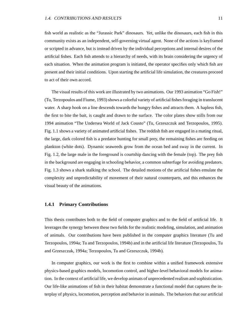
The visual results of this work are illustrated by two animations. Our 1993 animation “Go Fish!”
(Tu, Terzopoulos and Fiume, 1993) shows a colorful variety of artificial fishes foraging in translucent
water. A sharp hook on a line descends towards the hungry fishes and attracts them. A hapless fish,
the first to bite the bait, is caught and drawn to the surface. The color plates show stills from our
1994 animation “The Undersea World of Jack Cousto” (Tu, Grzeszczuk and Terzopoulos, 1995).
Fig. 1.1 shows a variety of animated artificial fishes. The reddish fish are engaged in a mating ritual,
the large, dark colored fish is a predator hunting for small prey, the remaining fishes are feeding on
plankton (white dots). Dynamic seaweeds grow from the ocean bed and sway in the current. In
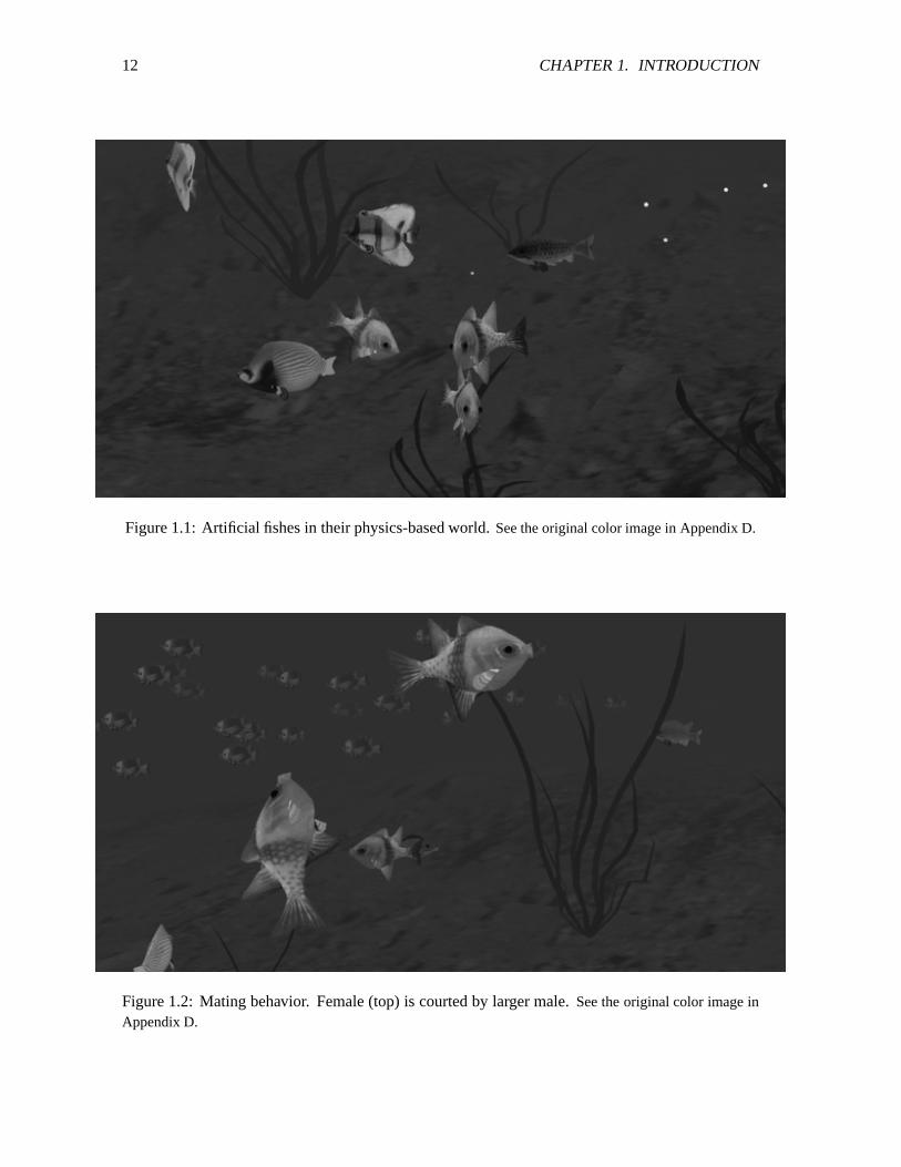
Fig. 1.2, the large male in the foreground is courtship dancing with the female (top). The prey fish
in the background are engaging in schooling behavior, a common subterfuge for avoiding predators.
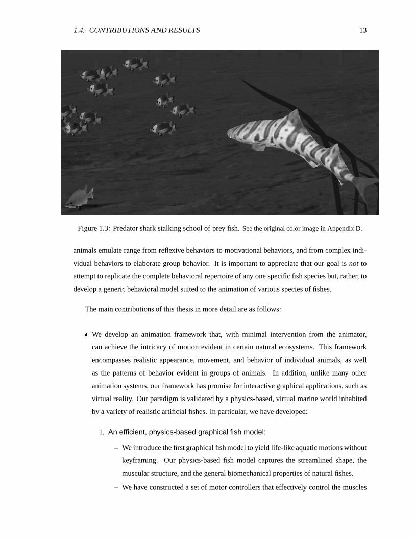
Fig. 1.3 shows a shark stalking the school. The detailed motions of the artificial fishes emulate the
complexity and unpredictability of movement of their natural counterparts, and this enhances the
visual beauty of the animations.
1.4.1 Primary Contributions
This thesis contributes both to the field of computer graphics and to the field of artificial life. It
leverages the synergy between these two fields for the realistic modeling, simulation, and animation
of animals. Our contributions have been published in the computer graphics literature (Tu and
Terzopoulos, 1994a; Tu and Terzopoulos, 1994b) and in the artificial life literature (Terzopoulos, Tu
and Grzeszczuk, 1994a; Terzopoulos, Tu and Grzeszczuk, 1994b).
In computer graphics, our work is the first to combine within a unified framework extensive
physics-based graphics models, locomotion control, and higher-level behavioral models for anima-
tion. In the context of artificial life, we develop animats of unprecedented realism and sophistication.
Our life-like animations of fish in their habitat demonstrate a functional model that captures the in-
terplay of physics, locomotion, perception and behavior in animals. The behaviors that our artificial
12 CHAPTER 1. INTRODUCTION
Figure 1.1: Artificial fishes in their physics-based world. See the original color image in Appendix D.
Figure 1.2: Mating behavior. Female (top) is courted by larger male. See the original color image inAppendix D.
1.4. CONTRIBUTIONS AND RESULTS 13
Figure 1.3: Predator shark stalking school of prey fish. See the original color image in Appendix D.
animals emulate range from reflexive behaviors to motivational behaviors, and from complex indi-
vidual behaviors to elaborate group behavior. It is important to appreciate that our goal is not to
attempt to replicate the complete behavioral repertoire of any one specific fish species but, rather, to
develop a generic behavioral model suited to the animation of various species of fishes.
The main contributions of this thesis in more detail are as follows:
� We develop an animation framework that, with minimal intervention from the animator,
can achieve the intricacy of motion evident in certain natural ecosystems. This framework
encompasses realistic appearance, movement, and behavior of individual animals, as well
as the patterns of behavior evident in groups of animals. In addition, unlike many other
animation systems, our framework has promise for interactive graphical applications, such as
virtual reality. Our paradigm is validated by a physics-based, virtual marine world inhabited
by a variety of realistic artificial fishes. In particular, we have developed:
1. An efficient, physics-based graphical fish model:
– We introduce the first graphical fish model to yield life-like aquatic motions without
keyframing. Our physics-based fish model captures the streamlined shape, the
muscular structure, and the general biomechanical properties of natural fishes.
– We have constructed a set of motor controllers that effectively control the muscles
14 CHAPTER 1. INTRODUCTION
of the artificial fish to generate realistic fish locomotion.
2. A perception model: The perception model simulates essential visual abilities and
limitations. It is equipped with a perceptual attention mechanism which is lacking
in previous perception models for animation. This perceptual attention mechanism is
essential for the realistic modeling of behavior.
3. A behavior model:
– A model of the internal motivations of an animal which comprises the innate
characteristics of an animal and its dynamic mental state.
– A set of behavior routines that implement a range of individual and group piscine
behaviors that are common across many species, such as collision avoidance (in the
presence of both static and moving obstacles), foraging, wandering, searching for
comfortable niches, fleeing, schooling and mating.
– An “intention generator” that arbitrates among different behaviors and controls the
perceptual attention mechanism.
� This thesis provides a new experimental environment for research in related disciplines, such
as computer vision and robotics. For example, artificial fishes have been used to design an
active computer vision system and evaluate its performance (Terzopoulos and Rabie, 1995)
and they have been employed to develop algorithms for learning locomotion and other motor
skills (Grzeszczuk and Terzopoulos, 1995). Artificial fishes are virtual robots situated in a
continuously dynamic 3D virtual world. They offer a much broader range of perceptual and
animation capabilities, lower cost, and higher reliability than can be expected from present-
day physical robots used in hardware vision (Terzopoulos, 1995). For at least these reasons,
artificial fishes in their dynamic world can serve as a proving ground for theories that profess
to account for the sensorimotor competence of animals.
1.4.2 Auxiliary Technical Contributions
� Interactive tools for capturing the realistic appearance of fishes from pictures: We have
developed a new tool for efficiently obtaining texture boundaries and coordinates for texture
mapping using a deformable mesh.
� A model of a marine environment:
– We model the physical properties of the hydrodynamic medium in order to simulate its
effect on fish motion.
1.5. THESIS OVERVIEW 15
– We have developed a physics-based model of seaweeds that can sway realistically in
simulated water current.
� Numerical algorithms for simulating the biomechanical fish models and their physics-
based environment: The simulator employs an efficient sparse matrix storage scheme and
a fast yet numerically stable semi-implicit Euler method. �� A graphical user interface:
– The interface enables the user to create his or her own virtual marine world. For example,
the user can decorate the marine environment with static objects and seaweeds, and can
specify the number, type, size, initial positions as well as individual habits (i.e. innate
behavioral characteristics) of artificial fishes.
– It allows the user to experiment with the physical properties of the fish, the hydrodynamic
medium, and the mental parameters of each fish.
– It controls the display of a binocular fish-view from the “eyes” of any chosen fish.
1.5 Thesis Overview
The thesis is organized as follows:
In Chapter 2 we review previous work upon which our research draws. At its lowest level of
abstraction, our work is an instance of physics-based graphics modeling. Therefore we first survey
physics-based modeling where we discuss two basic approaches: the constraint-based approach and
the motion synthesis approach. The modeling and control technique we employ in producing realistic
fish locomotion pertains to the latter. At a higher level of abstraction, our research is an instance
of advanced behavioral animation. We survey prior behavioral animation work and describe related
previous perception models developed for the purposes of animation. Then we proceed to discuss
the design of action selection mechanisms and review some related previous work in ALife/Animat
research.
In subsequent chapters, we describe in detail the animation system that we have developed. In
Chapter 3 we begin by presenting a functional overview of the artificial fish model.
�It supports the real-time simulation and wire-frame display (30 frames/second) of up to five swimming fish on a
Silicon Graphics R4400 Indigo�
Extreme desktop workstation. If real-time performance is not an issue, a huge numberof fish may be simulated and rendered photorealistically on such a system.

16 CHAPTER 1. INTRODUCTION
In Chapter 4 we describe the biomechanical model and how it achieves muscle-based hy-
drodynamic locomotion. Next, we develop a numerical simulation of the equations of motion.
Subsequently, the motor control of the physics-based artificial fish, derived from piscine biomechan-
ical principles, is presented. This includes the construction of the muscle motor controllers as well
as the pectoral fin motor controllers.
Chapter 5 describes our approach to constructing geometric display models that capture the form
and appearance of a variety of artificial fishes. An interactive, deformable contour tool is developed
and applied to map realistic textures over the fish bodies. Finally we explain how the geometric
display models are coupled to the biomechanical fish model to yield realistic animation.
In Chapter 6 we present the perception model employed within the artificial fish. In particular,
we describe the modeling of the perceptual attention mechanism and the use of motor preferences for
generating compromised actions. We present concrete examples of how perception guided behaviors
are synthesized. Possible extensions of our perception model are also discussed.
In Chapter 7 we discuss behavior modeling in the artificial fish. We describe the internal
motivations and action selection, which is carried out by an intention generator and a set of behavior
routines that are explained in detail. Results are presented to illustrate the various behaviors achieved
in three varieties of artificial fishes: pacifists, prey, and predators. We then analyze the properties of
the action selection mechanism that we have designed and possible extensions are suggested.
Chapter 8 discusses the modeling of the marine environment of the artificial fishes. In particular,
we describe the physics-based modeling of seaweeds, food particles and water currents.
In Chapter 9 we present the user interface that we have designed to facilitate the use of our
animation system.
In Chapter 10 we describe the animation results that we have achieved to date.
In Chapter 11 we review the contributions of the thesis, and list possible directions of future
research.
Chapter 2
Background
In this chapter, we review prior work in the fields of computer graphics and artificial life upon
which our research draws. Starting from the lowest level, physics-based graphics modeling, we
progressively survey related research on behavioral animation, including perception models for
animation and action selection mechanisms. We conclude by putting our work in perspective
relative to prior artificial life research on animats.
2.1 Physics-Based Modeling
At its lowest level of abstraction, our work is an instance of physics-based graphics modeling. This
approach involves constructing dynamic models of animated objects and computing their motions via
physical simulation. Physics-based modeling implies that object motions are governed by the laws
of physics, which leads to physically realistic animation. Moreover, this approach frees the animator
from having to specify many low-level motion details, since motion is synthesized automatically
by the physical simulation. This is evident especially when animating passive motion (i.e. motions
of inanimate objects)—the animator need only supply the initial state of the object and a physical
simulator automatically computes its motion by integrating the differential equations stemming from
Newton’s laws.
The success of physics-based modeling was demonstrated in modeling the movements of inani-
mate objects, such as deformable objects (Terzopoulos et al., 1987; Terzopoulos and Fleischer, 1988;
Witkin and Welch, 1990), chains (Barzel and Barr, 1988) and tree leaves (Wejchert and Haumann,
17
18 CHAPTER 2. BACKGROUND
1991). A substantial amount of research has also been concerned with the motion of animate objects,
such as humans and animals (Armstrong and Green, 1985; Wilhelms, 1987; Badler, Barsky and
Zeltzer, 1991; Hodgins et al., 1995).
An animator requires control over physics-based models in order to produce useful animations.
We can categorize physics-based control techniques into two approaches: the constraint-based
approach and the motion synthesis approach.
2.1.1 Constraint-based Approach
The constraint-based approach involves the imposition of kinematic constraints on the motions of
an animated object (Platt and Barr, 1988). For example, one may constrain the motion trajectories
of certain parts of a model to conform to user specified paths. Two techniques have been used
to calculate motions that satisfy constraints: the inverse dynamics technique and the constrained
optimization technique.
In inverse dynamics, the motion of an animated body is specified by solving the equations of
motion. A set of “constraint forces” (or torques) is computed, which causes the animated body to act
in accordance with the given constraints (Isaacs and Cohen, 1987; Barzel and Barr, 1988; Witkin and
Welch, 1990). The first two works deal with rigid bodies (for the special case of articulated figures),
the third with non-rigid structures. Using inverse dynamics, the resulting motions are physically
“correct” (in the sense that the animated body responds to forces in a realistic manner), but they
may still look unnatural with respect to any specific form of animal locomotion. For example, when
modeling the locomotion of a cat using inverse dynamics, the resulting motion may not resemble
that of a cat, but rather that of a robot. This is because, as was discussed in the previous chapter,
an animal’s movement not only depends on the Newtonian laws of motion but also is subject to
biomechanical principles. In particular, the locomotion of an animal is driven by its muscles, which
have limited strength. Therefore, contrary to the assumption of the inverse dynamics technique, a
real animal cannot produce arbitrary forces and torques so as to move along any pre-specified path.
The idea behind the constrained optimization technique is to represent motion in the state-time
space and then define an objective function or performance index and cast motion control as an
optimization problem (Witkin and Kass, 1988; Liu, Gortler and Cohen, 1994). The objective
function evaluates the resulting motion. The usual assumption is that motions requiring less energy
are preferable. An open-loop controller is synthesized by searching for values of the state space
2.1. PHYSICS-BASED MODELING 19
trajectory, the forces, and the torques that satisfy the constraints and minimize the objective function.
This is usually achieved by numerical methods that iteratively refine a user supplied initial guess
and that are often computationally expensive. Moreover, it is possible for the motion to be over-
constrained, in which case the optimization algorithm is given the responsibility of arbitrating
between the user defined constraints and the constraints induced by the laws of physics (Funge,
1995). Unfortunately, this means that the compromise solutions produced may not lead to visually
realistic motion, especially if the laws of physics are compromised.
2.1.2 Motion Synthesis Approach
The motion synthesis approach to physics-based control bears greater resemblance to how real
animals move. It synthesizes the muscles in natural animals as a set of actuators that are capable
of driving the dynamic model of a character to produce locomotion. Unlike inverse dynamics,
the motion synthesis approach can take into account the limitations of natural muscles, and unlike
constrained optimization, it guarantees that the laws of physics are never violated. It also allows
sensors to be incorporated into the animate models which establishes sensorimotor coupling or
closed-loop control. This in turn enables an animated character to automatically cope with the
richness of its physical environment. Since this approach can emulate natural muscles as actuators,
it is able to synthesize various locomotion modes found in real animals by emulating their muscle
control patterns. The quality of the results will of course depend upon the fidelity with which the
relevant biomechanical structures are modeled. The motion synthesis approach offers less direct
animator control than the constraint-based approach. For example, it is almost impossible to produce
motions of an animate body that exactly follow some given trajectory, especially for multi-body
models, such as human bodies (though humans do experience difficulty when attempting to produce
specific trajectories).
Several researchers have successfully applied the motion synthesis approach to animation (Miller,
1988; Terzopoulos and Waters, 1990; Lee, Terzopoulos and Waters, 1993; van de Panne and Fiume,
1993; Ngo and Marks, 1993). The artificial fish model that we develop is inspired by the surprisingly
effective model of snake and worm dynamics proposed by Miller (1988) and the face model proposed
by Terzopoulos and Waters (1990). �
An essential physical feature of the bodies of snakes and worms and of human faces is that
�An early draft of our model was developed based on a fish model that Caroline Houle (a former student at the graphics
lab) built for one of her course projects. We would like to acknowledge her contribution to our work.
20 CHAPTER 2. BACKGROUND
they are deformable. In both Miller’s and Terzopoulos and Waters’ works, this feature is efficiently
modeled by mass-spring systems. The springs are used to simulate simple muscles that are able
to contract by varying their rest lengths. Like these previous models, our fish model is a dynamic
mass-spring-damper system with internal contractile muscles that are activated to produce the desired
motions. Unlike these previous models, however, we simulate the system using a semi-implicit Euler
method which, although computationally more expensive than simple explicit methods, maintains
the stability of the simulation over the large dynamic range of forces produced in our simulated
aquatic world. Using mass-spring-damper systems, we also model the passive dynamic plants found
in the artificial fish habitat.
The major task in motion synthesis is to derive suitable actuator control functions, in particular
the time-varying muscle actuator activation functions for different modes of locomotion, such as
hopping or flying. When activated according to the corresponding function, each muscle generates
forces and torques causing motion of the actuated body parts. The aggregate motion of all body
parts forms the particular locomotion pattern. The derivation of actuator control functions becomes
increasingly difficult as the number of muscles involved in controlling the locomotion increases.
There are two approaches to deriving control functions: the manual construction of controllers and
optimization-based controller synthesis, also known as optimal control or learning.
Hand-Crafted Controllers
The manual construction of controllers involves hand crafting the control functions for a set of
muscles. This is often possible when the muscle activation patterns in the corresponding real animal
are well known. For example, in Miller’s (1988) work, the crawling motion of the snake is achieved
via a sinusoidal activation (i.e. contraction) function of successive muscle pairs along the body of
the snake. Another manually constructed controller for deformable models is that for controlling
facial muscles (Terzopoulos and Waters, 1990; Lee, Terzopoulos and Waters, 1995) for realistic
human facial animation, where a “facial action coding system” controller coordinates the actions of
the major facial muscles to produce meaningful expressions. Most manually constructed controllers
have been developed for rigid, articulated figures: Wilhelms (1987) developed “Virya” — one of the
earliest human figure animation system that incorporates forward and inverse dynamic simulation;
Raibert (1991) showed how useful parameterized controllers of hoppers, kangaroos, bipeds, and
quadrupeds can be achieved by decomposing the problem into a set of manually-manageable control
problems; Hodgins et al. (1995) used similar techniques to animate a variety of human motions
2.1. PHYSICS-BASED MODELING 21
associated with athletics; McKenna et al. (1990) produced a dynamic simulation of a walking
cockroach controlled by sets of coupled oscillators; Brooks (1991) achieved similar results for a six-
legged physical robot; Stewart and Cremer (1992) created a dynamic simulation of a biped walking
by defining a finite-state machine that adds and removes constraint equations. A good survey of
these sorts of approaches can be found in the book by Badler, Barsky and Zeltzer (1991).
Fish animation poses control challenges characteristic of highly deformable,muscular bodies, not
unlike those of snakes (Miller, 1988). We have devised a motor control system that achieves muscle-
based, hydrodynamic locomotion by simulating the dynamic interactions between the artificial
fish’s deformable body and its aquatic environment. To derive the muscle control functions for fish
locomotion, we have consulted the literature on marine biomechanics (Webb, 1989; Blake, 1983;
Alexander, 1992). The resulting parameterized controllers harness the hydrodynamic forces on fins
to achieve forward locomotion over a range of speeds, to execute turns, and to alter body roll, pitch,
and yaw so that the fish can move freely within its 3D virtual world.
The main drawback with manually constructed controllers is that they can be extremely difficult
and tedious to derive, especially for many-degree-of-freedom body motions. Moreover, the resulting
controllers may not be readily transferable to different models or systems; nevertheless, they can
serve as a good starting point for the optimization-based algorithms.
Optimization-Based Controller Synthesis
One can also use optimization techniques to derive control functions automatically. An optimization
algorithm tries to produce an optimal controller through repeated controller and trajectory generation,
rewarding better generated motions according to some user specified objective function. This
generate-and-test procedure resembles a trial-and-error learning process in humans and animals
and is therefore often referred to as “learning”. The resulting motion can be influenced indirectly
by modifying the objective function. We shall emphasize the difference between the optimization
algorithm that we are describing here and the constrained optimization technique mentioned earlier.
Here, the laws of physics are not treated as constraints and motion is represented in the actuator-time
space, rather than in the state-time space.
Since motions are always generated in accordance with the laws of physics, the optimization
algorithm is able to exploit the mechanical properties of the physics-based models as well as their
environment (Funge, 1995). Interesting modes of locomotion have been automatically discovered
22 CHAPTER 2. BACKGROUND
by using simple objective functions that reward low energy expenditure and distance traveled in
a fixed time interval (Pandy, Anderson and Hull, 1992; van de Panne and Fiume, 1993; Ngo and
Marks, 1993; Sims, 1994; Grzeszczuk and Terzopoulos, 1995). The resulting motions bear a
distinct qualitative resemblance to the way that animals with comparable morphologies perform
similar locomotion tasks. We shall emphasize, again, that the fidelity of the dynamic model is
critical to the realism of the resulting locomotion.
Although we have hand crafted the control functions for the artificial fish’s muscles, our model
is rich enough to allow such control functions to be obtained automatically through optimization, as
is demonstrated by the work of Grzeszczuk and Terzopoulos (1995).
2.2 Behavioral Animation
At a higher level of abstraction, we are interested in animating the behaviors of animals with an
intermediate level of behavioral complexity—somewhere in between the complexity of invertebrates
and of primates such as humans. In this regard, our research is an instance of behavioral animation,
where the motor actions of characters are controlled by algorithms based on computational models
of behavior (Reynolds, 1982; Reynolds, 1987). Consequently, an animator is able to specify motions
at a higher level, i.e. the behavior level, as opposed to specifying motion at the locomotion level
as is done in physics-based modeling. The animator is therefore concerned with the modeling of
individual behaviors. Behavioral animation approaches have been proposed to cope with the com-
plexity of animating anthropomorphic figures (Zeltzer, 1982), animating the synchronized motions
of flocks, schools, or herds (Reynolds, 1987) and interactive animation control (Wilhelms, 1990).
The seminal work in behavioral animation is that of Reynolds (1987). Creating vivid animations
of flocks of birds or schools of fish using conventional keyframing would require a tremendous
amount of effort from an animator. This is because, for example, while the overall motion of birds in
a flock is highly coordinated, individual birds have distinct trajectories. In keyframing, the animator
would have to script each bird’s motion carefully in each keyframe. By contrast, Reynolds proposed
a computational model of aggregate behavior. In his approach, each animated character, called a
“boid”, is an independent actor navigating its environment. Each boid has three simple behaviors:
separation, alignment and cohesion. A boid decides which behavior to engage in at any given time
based on its perception of the local environmental conditions, primarily the location of neighboring
boids. The motions of the individual boids are not scripted; rather, the organized flock is an emergent
2.2. BEHAVIORAL ANIMATION 23
property of the autonomous interactions between individual boid behaviors.
Although Reynolds’ model successfully achieves behavioral realism, it pays little attention to
locomotion realism. Because a kinematic model is used to control each boid’s locomotion, the
resulting motion of individual boids can be visually unrealistic and may not scale well to more
elaborate motion. Additionally, the behavioral model is limited by its simplicity. In particular, since
the goal is to animate flocking behavior, each boid is capable by design only of behaviors that are
useful to flocking. Our artificial fishes are “self-animating” in the sense of Reynolds’ work, but
unlike his procedural boid actors, they are more elaborate physical models that also have much
broader and more complex behavior repertoires.
2.2.1 Perception Modeling
Adaptive behavior is supported by perception of the environment as much as it is by action. It is
therefore crucial to model perception in artificial autonomous agents, � including animated animals,
humans and physical robots. Reynolds’ “boids” maintained flock formations through simple per-
ception of other nearby actors (Reynolds, 1987) while Mataric has demonstrated similar flocking
behaviors with physical robots (Mataric, 1994). The roach actor described by McKenna et al.
(1990) retreated when it sensed danger from a virtual hand. Renault et al. (1990) advocate a more
extensive form of synthetic vision for behavioral actors, including the automatic computation of
internal spatial maps of the world. The virtual humans in Thalmann’s work (1995) have simulated
simple visual, tactile and auditory sensors that enable them to perform tasks such as following a
leader or greeting each other and even playing ball games.
Perception modeling for animation, in general, is very different from that for robotics. In an
animation system, the detailed geometry of each scene can always be obtained by interrogating
the virtual world model, without extensive sensory information processing. In a robotics system,
however, this is not true. In fact, in order for a robot to obtain useful perceptual information, a visual
process needs to be synthesized. This will include algorithms to infer 3D geometry from images, to
identify shapes and to produce appropriate representations of objects, etc. On the other hand, in a
typical animation system, since a database of all graphical objects exists and is accessible, the main
purpose of modeling perception in animated figures is to enforce behavioral realism. This often
only requires that the perceptual capability of the animal be modeled, such as the field of view and
�An autonomous agent is an entity in a world that can act or behave on it own without explicit external control.
Humans and animals are examples of natural autonomous agents.
24 CHAPTER 2. BACKGROUND
occlusion. Reynolds’ model of boids (which only consists of simple modeling of limited field of
view) is a good example.
Our artificial fishes are currently able to sense their world through simulated visual perception
within a deliberately limited field of view. Subject to the natural limitations of occlusion, they can
sense lighting patterns, determine distances to objects, and identify objects by inquiring the world
model database. They are also equipped with secondary nonvisual modalities, such as the ability to
sense the local virtual water temperature. More importantly, unlike previous perception models for
animation, the artificial fish’s perception induces an attention mechanism. This mechanism allows
the fish to train its sensors in a task-specific way as well as to provide other important information
for producing convincing behavior. Our model of perception is proven to be effective in generating
realistic behaviors of the artificial fish.
2.2.2 Control of Behavior
Behavioral control mechanisms working in conjunction with the perception and the locomotion
control mechanisms make our artificial fishes autonomous agents.
To achieve a level of behavioral realism consistent with the locomotional abilities of artificial
fishes, it is prudent to consult the ethology literature (Tinbergen, 1950; Lorenz, 1973; McFarland,
1987; Adler, 1975). Tinbergen’s landmark studies of the three-spined stickleback highlight the
great diversity of piscine behavior, even within a single species. The artificial fishes’ behavior
repertoires are modeled after natural piscatorial behaviors common across several species. We
achieve the nontrivial patterns of behavior (including schooling behaviors as convincing as those
demonstrated by Reynolds) in stages. First, we implement primitive reflexive behaviors, such as
obstacle avoidance, that tightly couple perception to action (Braitenberg, 1984; Resnick, 1987).
Then, through an effective action selection mechanism, the primitive behaviors are combined into
motivational behaviors whose activation depends also on the artificial fish’s mental state, including
hunger, libido, and fear.
As the behavioral repertoire broadens, the issue of action selection becomes crucial. In the next
section we survey related prior work on the design of action selection mechanisms for autonomous
agents.
2.3. THE MODELING OF ACTION SELECTION 25
2.3 The Modeling of Action Selection
Designing autonomous agents has been one of the major concerns in several fields of research.
In software engineering, intelligent computer programs have been developed that can be viewed
as autonomous software agents. These programs automatically accomplish various software tasks
with little intervention from the user. In robotics, current research has concentrated on developing
autonomous mobile robots that can function successfully with little or no human monitoring. In
computer graphics, by modeling each animated character as an autonomous agent, complex ani-
mations can be produced with minimal intervention from the animator, as is demonstrated in this
thesis.
Any autonomous agent will encounter the problem of action selection. The task of action
selection (also known as behavior arbitration or behavioral choice) is to determine, from a set of
available actions, the most appropriate one based on the agent’s internal and external conditions.
Designing effective action selection mechanisms is a major endeavor in the design of autonomous
agents. To this end, two questions need to be answered first: “what do we mean by an action?” and
“what do we mean by the most appropriate action?”.
2.3.1 Defining Action
The term “action” has been used widely in the ethology, psychology and robotics literature, some-
times with quite different meanings. A popular definition of action, in the context of action selection
in animals, is given by Tyrrell (1992): an action refers to one of the mutually exclusive entities at the
level of the behavioral final common path (McFarland and Sibly, 1975). The level of the behavioral
final common path is the lowest level of control in an animal or agent’s control system, whereby all
behaviors are expressed. However meaningful and accurate from an ethologist’s point of view, this
definition leads to a certain degree of confusion from a designer’s point of view. More precisely,
it gives the impression that an action is “a movement”, hence the action selection mechanism in
an anthropomorphic robot, for example, is responsible for determining the detailed movements of
every muscle. As a result, one cannot help wondering how the action selection mechanism is any
different from the whole control system of an agent. An alternative is therefore to define an action as
a motor skill, such as “move forward” or “turn to the right”. � Depending on the mechanical model
of an agent, each of its actions may require a simple single movement of a single actuator or muscle,
�In fact, although often not explicitly stated, actions are most commonly defined as motor skills in robotics.
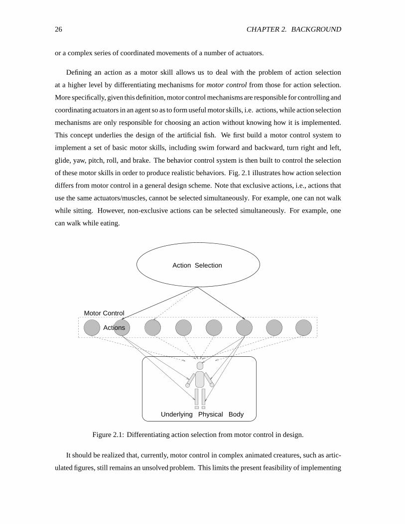
26 CHAPTER 2. BACKGROUND
or a complex series of coordinated movements of a number of actuators.
Defining an action as a motor skill allows us to deal with the problem of action selection
at a higher level by differentiating mechanisms for motor control from those for action selection.
More specifically, given this definition, motor control mechanisms are responsible for controlling and
coordinating actuators in an agent so as to form useful motor skills, i.e. actions, while action selection
mechanisms are only responsible for choosing an action without knowing how it is implemented.
This concept underlies the design of the artificial fish. We first build a motor control system to
implement a set of basic motor skills, including swim forward and backward, turn right and left,
glide, yaw, pitch, roll, and brake. The behavior control system is then built to control the selection
of these motor skills in order to produce realistic behaviors. Fig. 2.1 illustrates how action selection
differs from motor control in a general design scheme. Note that exclusive actions, i.e., actions that
use the same actuators/muscles, cannot be selected simultaneously. For example, one can not walk
while sitting. However, non-exclusive actions can be selected simultaneously. For example, one
can walk while eating.
Motor Control
Underlying Physical Body
Action Selection
Actions
Figure 2.1: Differentiating action selection from motor control in design.
It should be realized that, currently, motor control in complex animated creatures, such as artic-
ulated figures, still remains an unsolved problem. This limits the present feasibility of implementing
2.3. THE MODELING OF ACTION SELECTION 27
the above described behavior control scheme in such creatures. However, this should not indicate the
lack of generality of the control scheme for we believe that the separation of action selection from
motor control is necessary in achieving high level behaviors in most creatures, especially complex
ones.
2.3.2 Goals and Means
The most appropriate action can be evaluated with respect to the goal of action selection. Animals
in the wild often face hazardous situations. The appropriate choice of actions is crucial to their long
term survival. Therefore, according to Dawkins (1989), the ultimate goal of action selection for
animals is to choose successive actions (or behaviors) so as to maximize the number of copies of its
genes in future generations. That is to say, the ultimate goal is to survive and to reproduce. This
goal breaks down to more immediate, day to day behavioral needs. For a robot, the action selection
problem entails maintaining the safety of the robot while pursuing the successful completion of the
tasks it has been assigned. For a virtual animal (or an autonomous animated creature in general),
the goal of action selection is to achieve satisfactory behavioral realism. Since a mathematical
representation of the above goals would be extremely complex, we may not be able to build action
selection mechanisms via numerical methods, such as optimization. This makes the problem of
deriving action selection mechanisms a design problem and hence the main issue is to come up with
the corresponding design criteria (Werner, 1994; Maes, 1991a; Tyrrell, 1992).
Although the goal of action selection in a real animal seems different from that in a virtual
animal, they are in fact similar. The action selection mechanisms in animals allow them to take
appropriate actions in the face of uncertainty. This is what we refer to as rational, adaptive behavior.
When we say the behavior of a virtual animal looks realistic, we generally mean that the behavior
it exhibits makes sense. Like a real animal, the virtual animal “knows” to avoid hazards, to exploit
opportunities and to reasonably allocate resources, etc. Our approach to achieving such realism in
animation involves identifying the important principles by which animals select actions, especially
priorities between different behaviors, and employing these principles as the design criteria for
building action selection mechanisms in virtual animals.
28 CHAPTER 2. BACKGROUND
2.3.3 Previous Work
In prior behavioral animation work, such as that of Reynolds (1987), only stimulus-driven action
selection process is modeled. For example, the three sub-behaviors of a flocking boid are activated
directly by environmental conditions. If the environmental conditions for more than one sub-
behavior occur, the one with the highest weight gets chosen (each sub-behavior is associated with a
weighting factor that reflects its importance). Comparably, Sun and Green (1993) specify the action
selection of a synthetic actor through a set of “relations” each of which is a mapping from an external
stimulus to a response of the actor.
Analogous strategies have been taken in robotics. Representative examples include the rule-
based mechanism in “Pengi” developed by Agre and Chapman (1987); and reactive systems and
systems with emergent functionality, such as those proposed by Kaelbling (1987), Brooks (1986) and
Anderson (1990). These mechanisms have the main advantage of coping well with contingencies
in the environment since actions are more or less directly coupled with external stimuli. However,
as Tyrrell (1993a) points out:
… while we realise that many traditional planning approaches are unsuitable for action
selection problems due to their rigidness and disregard of the uncertainty of the envi-
ronment, we also realize that stimulus-driven mechanisms err in the opposite direction.
In particular, these mechanisms do not model the agent’s internal state thus cannot take into account
the agent’s motivations. They are therefore limited in dealing with more sophisticated action
selection problems faced by agents with multiple high-level (probably motivational) behaviors, such
as those faced by most animals.
Being well aware of the aforementioned problems, researchers in ALife and related fields (e.g.
robotics) have come up with various implementation schemes for action selection in animats that
takes into account both internal and external stimuli. This body of work provides valuable reference
to our design of the behavior control system of the artificial fish.
Maes (1990; 1991a) proposed a distributed, non-hierarchical implementation of action selection,
called a “behavior choice network”. The results demonstrate that this model possesses certain
properties that are believed to be important to action selection in real animals, such as persistence
in behavior, opportunism and satisfactory efficiency. However, while the distributed structure offers
good flexibility, it also causes some problems. For example, convergence to a correct choice of
2.3. THE MODELING OF ACTION SELECTION 29
behavior is hard to guarantee. Using a similar architecture to that of Maes’ network, Beer and Chiel
(1991) proposed a neuroethology-based implementation of an artificial nervous system for simple
action selection in a robot insect.
Along the line of Maes’ and Beer’s work, others have also proposed various different network-
type of action selection mechanisms. For instance, Sahota’s (1994) mechanism allows behaviors to
“bid”, and the behavior with the highest bid represents the most appropriate choice.
A common attribute of the above mechanisms (and many others) is the use of a winner-takes-all
selection/arbitration process, where the final decision is made exclusively by the winning action or
behavior. While this offers highly focussed attention and hence efficiency, it ignores the importance
of generating compromised actions. The ability to compromise between different, even conflicting,
desires is evident in natural animals. Tyrrell (1993b) emphasized this particular aspect of animal
behavior in the implementation of what is known as free-flow hierarchies. A free-flow hierarchy im-
plements compromised actions (Rosenblatt and Payton, 1989) within a hierarchical action selection
architecture similar to those proposed by early ethologists, such as Tinbergen (1951). The winner
is only chosen at the very bottom level of the hierarchy. Simulation results (Tyrrell, 1993a) show
that free-flow hierarchies yield favorable choices of action compared to other mechanisms, such as
Maes’. A similar scheme is used to design the brains of the pets in Coderre’s (1987) PetWorld. The
main difference between the decision-making (or data-flow) hierarchy in PetWorld and a free-flow
hierarchy is that, in the former, sensory data flows from the bottom of the hierarchy to the top
while in the latter, it flows top down. The major drawback of such an implementation is its high
complexity, hence inefficiency, due to the large amount of computations required.
The behavior system of the artificial fish incorporates both stimulus-driven mechanisms and
motivation-based mechanisms for action selection. As a result, the fish possesses a level of behavioral
capacity to achieve coherence among a number of complex behaviors. In this regard, our work is
compatible with the work by Coderre (1987), Maes (1990; 1991a) and Tyrrell (1993b).
Our implementation is similar to that of Tyrrell in that it employs a top-down hierarchical structure
and real valued sensory readings, and it can generate compromised actions. Unlike Tyrrell’s model,
our mechanism employs essentially a winner-takes-all selection process and allows only certain
losing behaviors to influence the execution of the winning behavior. This way action selection
is carried out much more efficiently than a free-flow hierarchy. Since more than one behaviors
influence the selection of the detailed actions taken for accomplishing the chosen behavior, the
final choices of actions are preferable to that generated by a conventional winner-takes-all process.
30 CHAPTER 2. BACKGROUND
Moreover, the majority of the previous action selection models (including the aforementioned ones)
are based on a discrete 2D world which simplifies the problem by greatly restricting legal choice of
motor actions. Our model, however, is based on a continuous 3D environment in which the animated
animals perform continuous motions.
2.3.4 Task-level Motion Planning
When one attempts to animate advanced animals, such as humans, it becomes necessary to incor-
porate more abstract action selection mechanisms, such as mechanisms based on reasoning. This
approach involves using AI techniques and is termed task-level motion planning (a good reference
book on this subject is the book by Magnenat-Thalmann and Thalmann (1990)); The most represen-
tative animation work along this line is that by Badler and his group who animated a human figure
’Jack’ (Badler, Phillips and Webber, 1993). The planner takes as input Jack’s initial state and a 3D
representation of his world and generates as output a series of actions necessary for accomplishing
an assigned task, such as “go and get some ice cream”.
While planning ability certainly is one of the most important characteristics in human behavior
(and hence is important to model for animations of humans), it is not known as a common feature in
most animals lower on the evolutionary ladder than primates. Rather, animal behavior is believed to
rest on the more primitive and more fundamental faculty of reactive or adaptive behavior (Tinbergen,
1951; Manning, 1979; McFarland, 1993a). Adaptive behavior enables animals to be autonomous
and to survive in uncertain and dynamic environments. Our approach to behavioral animation
reflects the adaptiveness of animal behavior. (Note that we are not referring to adaptiveness in
the sense of learning nor evolutionary adaptation, but rather, to the ability to select appropriate
behaviors according to the perceived situation.) In our approach, we gain high level control through
the construction of a model of adaptive behavior where the actions of an artificial animal result from
its active interaction with the world as guided by its perception.
2.4 Summary
Our approach to developing artificial animals is consistent with the “animat” approach proposed by
Wilson (Wilson, 1990). To render our computational model visually convincing, we attempt also to
capture, with reasonable fidelity, the appearance and physics of the animal and its world. Artificial
2.4. SUMMARY 31
fishes may be viewed as animats of high sophistication. They are autonomous virtual robots situated
in a continuous, dynamic 3D virtual world. Their functional design, including motor control,
perceptual modeling, and behavioral simulation presents hurdles paralleling those encountered in
building physical autonomous agents (see, e.g., the compilation by Maes (1991b)). Previously, the
most complex animats were inspired by insects. Brooks (see (Brooks, 1991)) describes a physical
insect robot “Genghis”, bristling with sensors, that can locomote over irregular terrain, while Beer
develops a virtual counterpart, a cockroach with simple behaviors in a 2D world (Beer, 1990; Beer
and Chiel, 1991). Our work tackles animal behavior more complex than those modeled in existing
work such as the above. To deal with the broad behavioral repertoire of fishes, we exploit ideas from
physics-based graphics modeling, from biomechanics, from behavioral animation, from autonomous
agent studies and from ethology.

32 CHAPTER 2. BACKGROUND
Chapter 3
Functional Anatomy of an Artificial Fish
As we discussed in the preceding chapter, there are diverse aspects to the realistic modeling of an
artificial animal, from superficial appearance to internal functionality. It is helpful to think of the
artificial fish model as consisting of three submodels:
1. A graphical display model that uses geometry and texture mapping to capture the form and
appearance of any specific real fish.
2. A biomechanical model that captures the physical and anatomical structure of the fish’s body,
including its muscle actuators, and simulates its deformation and physical dynamics.
3. A brain model that is responsible for motor control, perception control and behavior control
of the fish.
Each of the three submodels will be developed in detail in the coming chapters. Fig. 3.1 presents
a functional overview of the artificial fish. As the figure illustrates, the body of the fish harbors its
brain. The brain itself consists of three control centers: the motor center, the perception center, and
the behavior center. These centers are part of the motor, perception, and behavior control systems
of the artificial fish. The function of each of these systems will be previewed next.
33
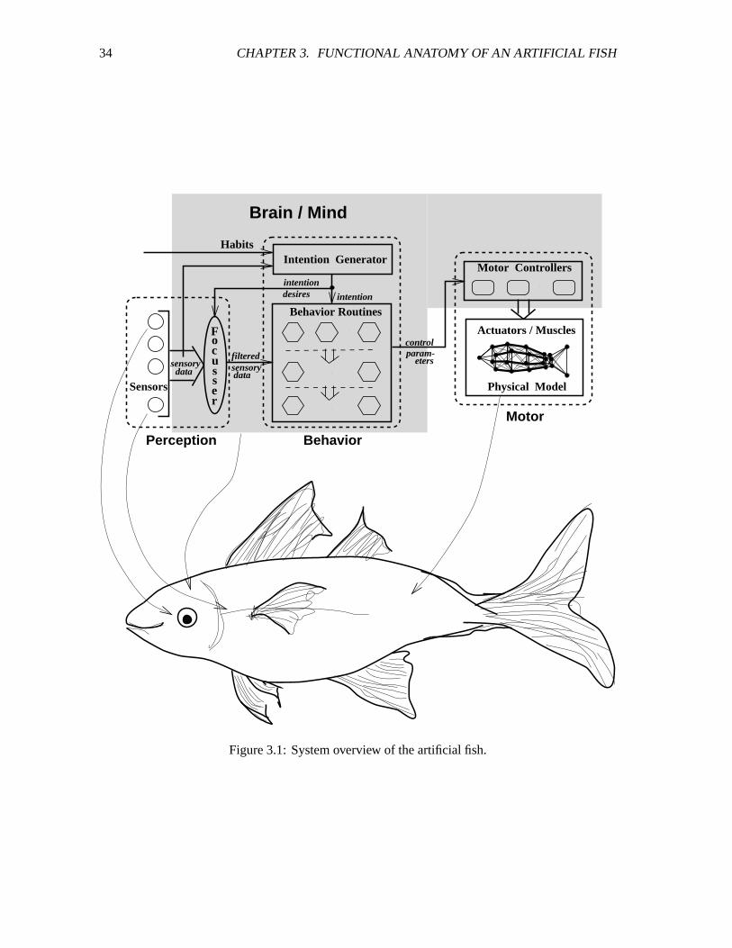
34 CHAPTER 3. FUNCTIONAL ANATOMY OF AN ARTIFICIAL FISH
Motor
BehaviorPerception
Sensors
filtered
Motor Controllers
Actuators / Muscles
Physical Model
Brain / Mind
desiresintention
intention
Behavior Routines
param-
data
eterssensorydata
Intention Generator
control
Habits
sensory
F
suco
s
re
Figure 3.1: System overview of the artificial fish.
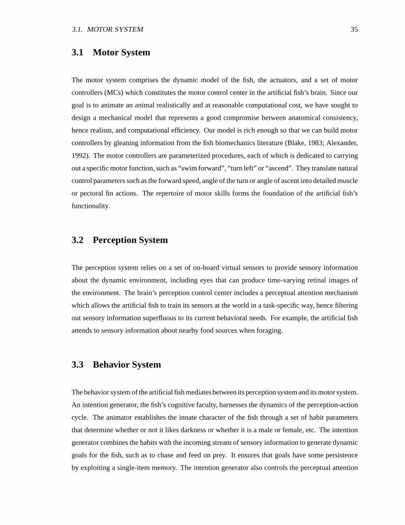
3.1. MOTOR SYSTEM 35
3.1 Motor System
The motor system comprises the dynamic model of the fish, the actuators, and a set of motor
controllers (MCs) which constitutes the motor control center in the artificial fish’s brain. Since our
goal is to animate an animal realistically and at reasonable computational cost, we have sought to
design a mechanical model that represents a good compromise between anatomical consistency,
hence realism, and computational efficiency. Our model is rich enough so that we can build motor
controllers by gleaning information from the fish biomechanics literature (Blake, 1983; Alexander,
1992). The motor controllers are parameterized procedures, each of which is dedicated to carrying
out a specific motor function, such as “swim forward”, “turn left” or “ascend”. They translate natural
control parameters such as the forward speed, angle of the turn or angle of ascent into detailed muscle
or pectoral fin actions. The repertoire of motor skills forms the foundation of the artificial fish’s
functionality.
3.2 Perception System
The perception system relies on a set of on-board virtual sensors to provide sensory information
about the dynamic environment, including eyes that can produce time-varying retinal images of
the environment. The brain’s perception control center includes a perceptual attention mechanism
which allows the artificial fish to train its sensors at the world in a task-specific way, hence filtering
out sensory information superfluous to its current behavioral needs. For example, the artificial fish
attends to sensory information about nearby food sources when foraging.
3.3 Behavior System
The behavior system of the artificial fish mediates between its perception system and its motor system.
An intention generator, the fish’s cognitive faculty, harnesses the dynamics of the perception-action
cycle. The animator establishes the innate character of the fish through a set of habit parameters
that determine whether or not it likes darkness or whether it is a male or female, etc. The intention
generator combines the habits with the incoming stream of sensory information to generate dynamic
goals for the fish, such as to chase and feed on prey. It ensures that goals have some persistence
by exploiting a single-item memory. The intention generator also controls the perceptual attention

36 CHAPTER 3. FUNCTIONAL ANATOMY OF AN ARTIFICIAL FISH
mechanism to filter out sensory information unnecessary to accomplishing the goal in hand. For
example, if the intention is to eat food, then the artificial fish attends to sensory information related
to nearby food sources. At every simulation time step, the intention generator activates behavior
routines that input the filtered sensory information and compute the appropriate motor control
parameters to carry the fish one step closer to fulfilling the current intention. Primitive behavior
routines, such as obstacle avoidance, and more sophisticated motivational behavior routines, such
as mating, are the building blocks of the behavioral repertoire of the artificial fish.
In the subsequent chapters, we detail the modeling of the aforementioned subsystems of the
artificial fish.
Chapter 4
Biomechanical Fish Model and
Locomotion
This chapter discusses the motor system of the artificial fish (see Fig. 4.1). In particular, we describe
the physics-based fish model and how it achieves locomotion. The biomechanical model we develop
is simple, but it is nonetheless effective for realistically animating fish locomotion. We start by
presenting the structure of the dynamic fish model, then introduce the dynamics of this model and
the simulated aquatic environment. The numerical method employed for solving the differential
equations of motion of the fish model is discussed next. Subsequently we describe the biomechanics-
based modeling and control of the fish’s locomotion, paying special attention to the construction of
the motor controllers. This includes the abstraction of the muscle movements for useful locomotion
and the functional modeling of the pectoral fins.
4.1 Discrete Physics-Based Models
The bodies of most fishes are highly deformable structures. We construct our dynamic fish model
using a deformable mass-spring-damper system. There are several reasons for this choice:
� A mass-spring-damper model is a simple discrete mechanical structure capable of nonlinear,
nonrigid dynamics.
37
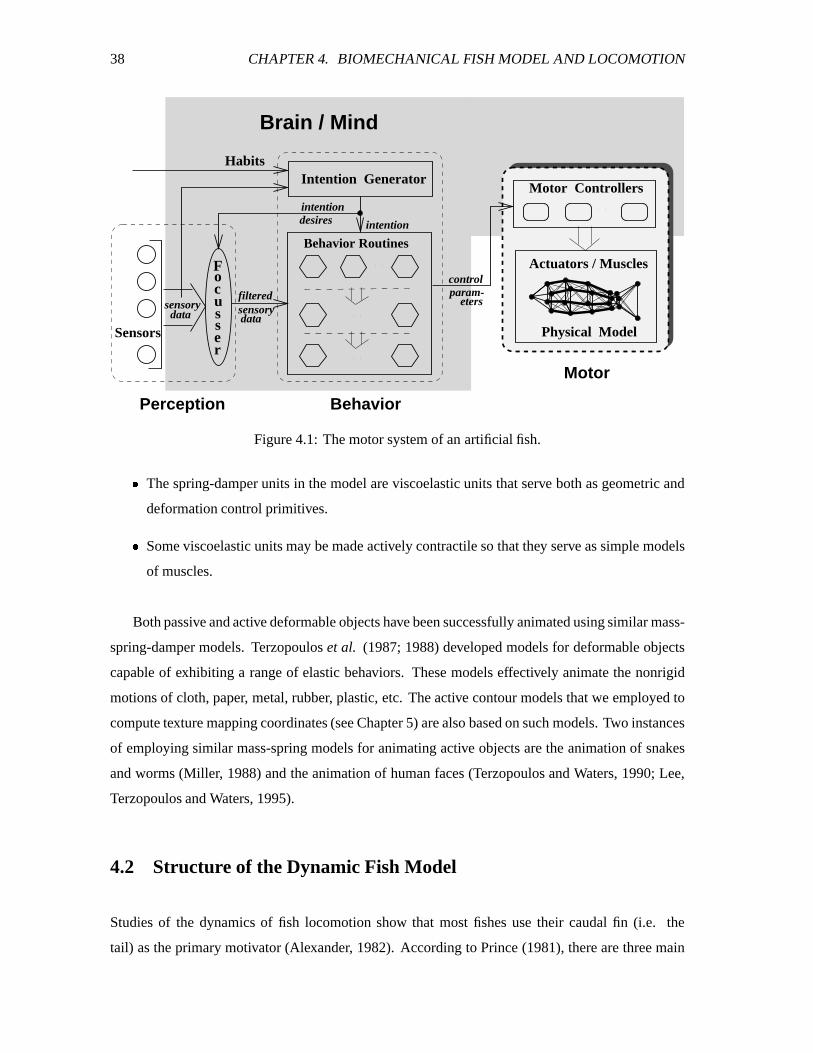
38 CHAPTER 4. BIOMECHANICAL FISH MODEL AND LOCOMOTION
Motor
BehaviorPerception
eterssensorydata
sensorydata
Sensors
filtered
Habits
Physical Model
Behavior Routinesintention
intentiondesires
Actuators / Musclescontrol
Intention Generator
param-
Brain / Mind
Motor Controllers
Focusser
Figure 4.1: The motor system of an artificial fish.� The spring-damper units in the model are viscoelastic units that serve both as geometric and
deformation control primitives.� Some viscoelastic units may be made actively contractile so that they serve as simple models
of muscles.
Both passive and active deformable objects have been successfully animated using similar mass-
spring-damper models. Terzopoulos et al. (1987; 1988) developed models for deformable objects
capable of exhibiting a range of elastic behaviors. These models effectively animate the nonrigid
motions of cloth, paper, metal, rubber, plastic, etc. The active contour models that we employed to
compute texture mapping coordinates (see Chapter 5) are also based on such models. Two instances
of employing similar mass-spring models for animating active objects are the animation of snakes
and worms (Miller, 1988) and the animation of human faces (Terzopoulos and Waters, 1990; Lee,
Terzopoulos and Waters, 1995).
4.2 Structure of the Dynamic Fish Model
Studies of the dynamics of fish locomotion show that most fishes use their caudal fin (i.e. the
tail) as the primary motivator (Alexander, 1982). According to Prince (1981), there are three main
4.2. STRUCTURE OF THE DYNAMIC FISH MODEL 39
types of caudal propulsion. In the first type, demonstrated by rigid-bodied and armored fish, the
tail and a very small part of the adjacent body is used. In the second type, demonstrated by active
swimmers such as herring, mackerel, salmon, etc., at least half the body is flexed. In the third type,
demonstrated by eels, almost the entire body length is deformed in an undulating action.
We would like to develop the simplest biomechanical fish model whose locomotion synthesizes
the second kind of caudal swimming pattern. To this end, we designed a mass-spring-damper model
consisting of 23 nodal point masses and 91 spring-damper units illustrated in Fig. 4.2. The units
serve as uniaxial deformable elements whose arrangement maintains the structural stability of the
body while allowing it to flex. The faces of the nodes are cross-strutted with elements to resist
twisting and shearing.
Twelve of the deformable units span the length of the body and serve as simple muscles (the bold
lines in Fig. 4.2). These muscles form three muscular segments, each with two pairs of muscles,
one on either side of the body. The posterior two segments which cover half of the length of the
fish body are used for swimming and the anterior two segments are used for turning. This muscle
distribution and usage approximates that found in most natural fish (Webb, 1984).
The shape of a fish directly affects the way it locomotes since the hydrodynamic forces are
shape-dependent (more details can be found in Section 4.4). Active natural fishes have evolved
a streamlined shape, where their greatest body diameter is just under the midpoint of their bodies
(Prince, 1981). The streamlined shape of the body reduces water turbulence that retards forward
motion. The large surface area of the mid-body induces relatively large hydrodynamic forces
on the sides which mitigate lateral instability. Since we want the artificial fish to be able to
locomote realistically in simulated water, it is important that we design its shape in accordance to
the streamlined shape of natural fishes. Fig. 4.3 shows the top and the side view of the physics-based
fish model (without the cross-strut viscoelastic units).
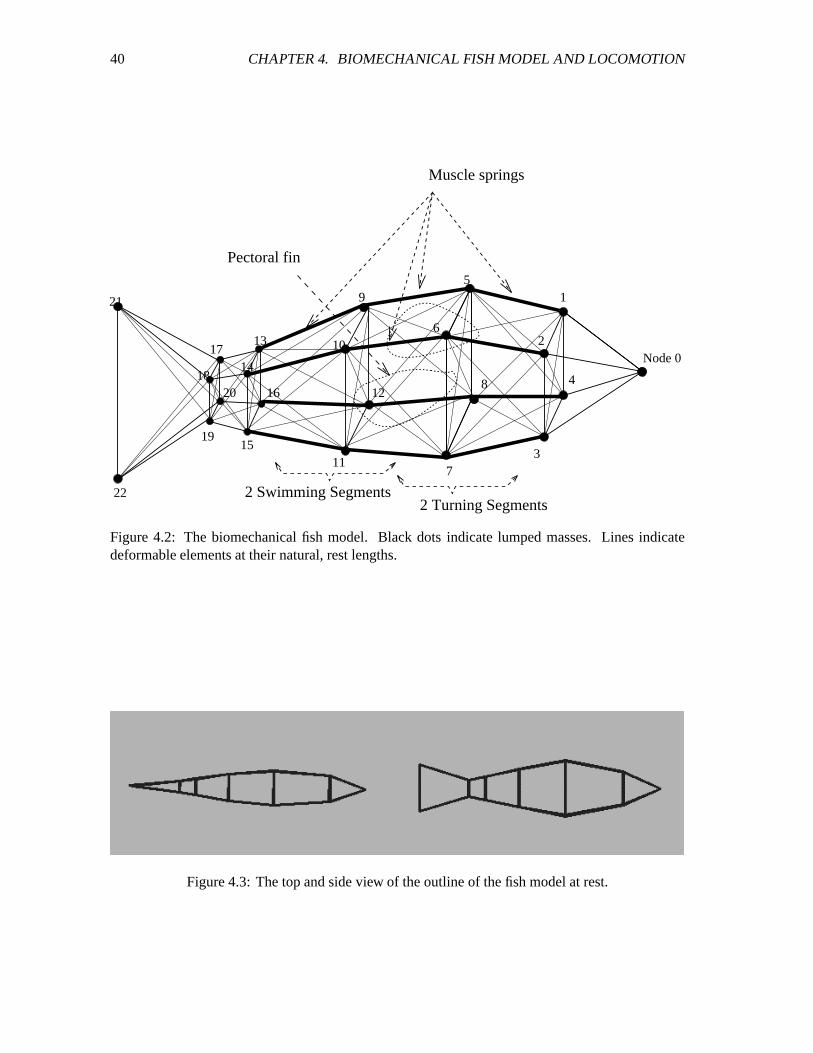
40 CHAPTER 4. BIOMECHANICAL FISH MODEL AND LOCOMOTION
2 Swimming Segments2 Turning Segments
Muscle springs
Node 0
1
2
3
4
5
6
7
8
9
10
11
13
15
16
17
18
19
20
21
22
14
12
Pectoral fin
Figure 4.2: The biomechanical fish model. Black dots indicate lumped masses. Lines indicatedeformable elements at their natural, rest lengths.
Figure 4.3: The top and side view of the outline of the fish model at rest.
4.3. MECHANICS 41
4.3 Mechanics
We will now specify the mechanics of the mass-spring-damper model. Let node�
have mass ��� ,position �������� ������������������������������� , velocity ������� "!#�$��%&!' , and acceleration (������ "!*)�����%+!#,) .4.3.1 Viscoelastic Units
Each spring-damper pair forms a uniaxial Voigt viscoelastic unit (Fig. 4.4) that simulates, in a simple
way, the viscoelasticity of biological tissue (Terzopoulos and Fleischer, 1988). A Voigt viscoelastic
unit comprises an elastic element (a Hookean spring with nonzero rest length) in parallel with a
viscous element (a dashpot). Let -.�0/ denote the Voigt viscoelastic unit connecting node�
to node 1 .
It has elasticity constant 2��0/ , viscosity constant 3��0/ and rest length 45�0/����� (the rest length of the muscle
units may change over time in order to activate motion, see Section 4.6). The deformation of the
elastic component is 67� /���� "8��0/����:9;45�0/���� , where 8��0/���� =<5<0>��0/����?<5< and >��0/�����@ A�./����:9B�$���� .According to Hooke’s law, the elastic force that the spring component of -.�0/ exerts on node
�isC&D�0/ ���� 2 �0/ 6 �0/ ����E> �0/87� / F
The same spring also exerts the force 9 C D�0/ on node 1 .
The linear viscous component of -.�0/ is a dashpot (see Fig. 4.4(b)). It exerts a viscous forceC�G� / ���
on node�
which is proportional to H8 �0/ ��� :C G�0/ ��� 3��0/$H8��0/����E>�� /8��0/where H8��0/���� I��JK�0/.LM>�� /7��%&87� / and JN� /���� O�./����&9P���,���� defines the difference between the velocities
of node�
and 1 . The same component exerts the force 9 CQG�0/ ��� on node 1 .
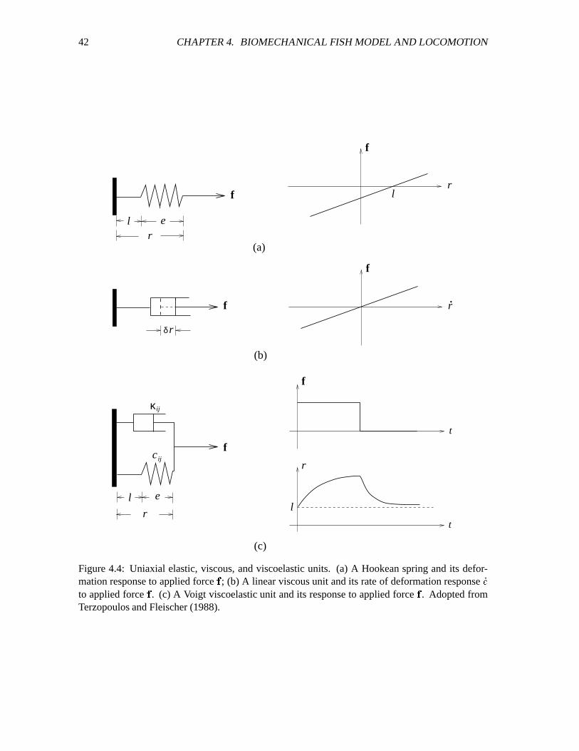
42 CHAPTER 4. BIOMECHANICAL FISH MODEL AND LOCOMOTION
f
t
ij
ij
el
δ
f
f
(a)
(b)
(c)
f
f.r
r
r
elr
l
t
l
c
κ
f
r
r
Figure 4.4: Uniaxial elastic, viscous, and viscoelastic units. (a) A Hookean spring and its defor-mation response to applied force
C; (b) A linear viscous unit and its rate of deformation response H6
to applied forceC. (c) A Voigt viscoelastic unit and its response to applied force
C. Adopted from
Terzopoulos and Fleischer (1988).
4.3. MECHANICS 43
Given the above derivations of the elastic and viscous component forces, the total force exerted
by the viscoelastic unit -.�0/ on node�
isC+R� / ���@ C D�0/ �����S C G� / ���@ "TU� /����E>��0/����where TU� /���� 2��0/�6��0/+���KSV3��0/$H8��0/����8 �0/ (4.1)
defines the effective stiffness of -.�0/ .Newtonian equations of motion
The generalized Newtonian equations of motion governing the dynamic fish model take the form of
a set of coupled second-order ordinary differential equations:
����W��������S;XY����� C�Z� ����[ � "\�� F5F5F ��]#]�� (4.2)
where X^���� �9�_/7`?aNb C R�0/ ����@ c9I_/�`�aNb T+�0/�����E>��0/is the net internal force on node
�due to the viscoelastic units connecting it to nodes 1edgfh� , wherefh� is the index set of neighboring nodes. Finally,
C Z� is the external (hydrodynamic) force on node�.
Biomechanical Properties
Efficient locomotion depends on the distribution of the weight and the muscle strength in an animal’s
body. For example, fish with heavy heads or tails will swim less efficiently and less gracefully than
fish with relatively light heads and tails, while fish with either too weak or too stiff muscles will also
suffer some degree of motor incompetence. The weight and the muscle strength distributions of the
physics-based artificial fish are characterized by the ��� and the 2�� / of the model, respectively. We
set these physical parameters of the model such that the corresponding distributions along the fish
body are biologically plausible. For example, the nodes that form the head and the tail of the fish
have less mass than those that form the middle part of the body.
The values of parameters used in our simulation are listed in Table 4.1 and Table 4.2.
44 CHAPTER 4. BIOMECHANICAL FISH MODEL AND LOCOMOTION
Node�
Attributes� "\ , iQjlk � kIiQm ���$ �i F iiPk � kVn , m^k � kIi�] ���$ "o F op k � kOq � � �i#i F \� "]�i#��]#] ���$ "\ F i�o pTable 4.1: The mass distribution of the artificial fish. Refer to Fig. 4.2.
Viscoelastic unit -.�0/ AttributesCross units, e.g. - ),r 2��0/s "j#q F \Muscle units: itk � kuiQ]��N1Y � S;n 2 �0/ "]#q F \Remaining units, e.g. -Nv ) 2��0/s "j#\ F \All units -w� / 3x� /y z\ F i
Table 4.2: The elasticity and viscosity constants of the artificial fish. Refer to Fig. 4.2.
Note that the elasticity constants are made large enough to provide the fish’s body with the
structural integrity that it requires for effective swimming. { However, this results in a rather stiff
dynamic system that needs a stable numerical solver to simulate its dynamics.
4.4 Muscles and Hydrodynamics
An artificial fish moves as a real fish does: by contracting its muscles. If -.�0/ is a muscle, it is
contracted by decreasing its rest length 4 �0/ . The characteristic undulation of the fish tail can be
achieved by periodically contracting the swimming segment muscles on one side of the body while
relaxing their counterparts on the other side. We will develop the motor controllers that produce this
muscle coordination in Section 4.6.
When the fish tail swings, it sets in motion a volume of water. The inertia of the displaced
water produces a reaction force normal to the fish’s body and proportional to the volume of water
displaced per unit time, which propels the fish forward (Fig. 4.5).
|More specifically, referring to Table 4.2, the cross viscoelastic units maintain the streamlined integrity of the fish
hence have the highest elasticity constants },~ ���g�����0� ; The muscles have elasticity constants },~ �$�����7� � , and },~ �������7� �for the remaining viscoelastic units that form other structures, such as the head.
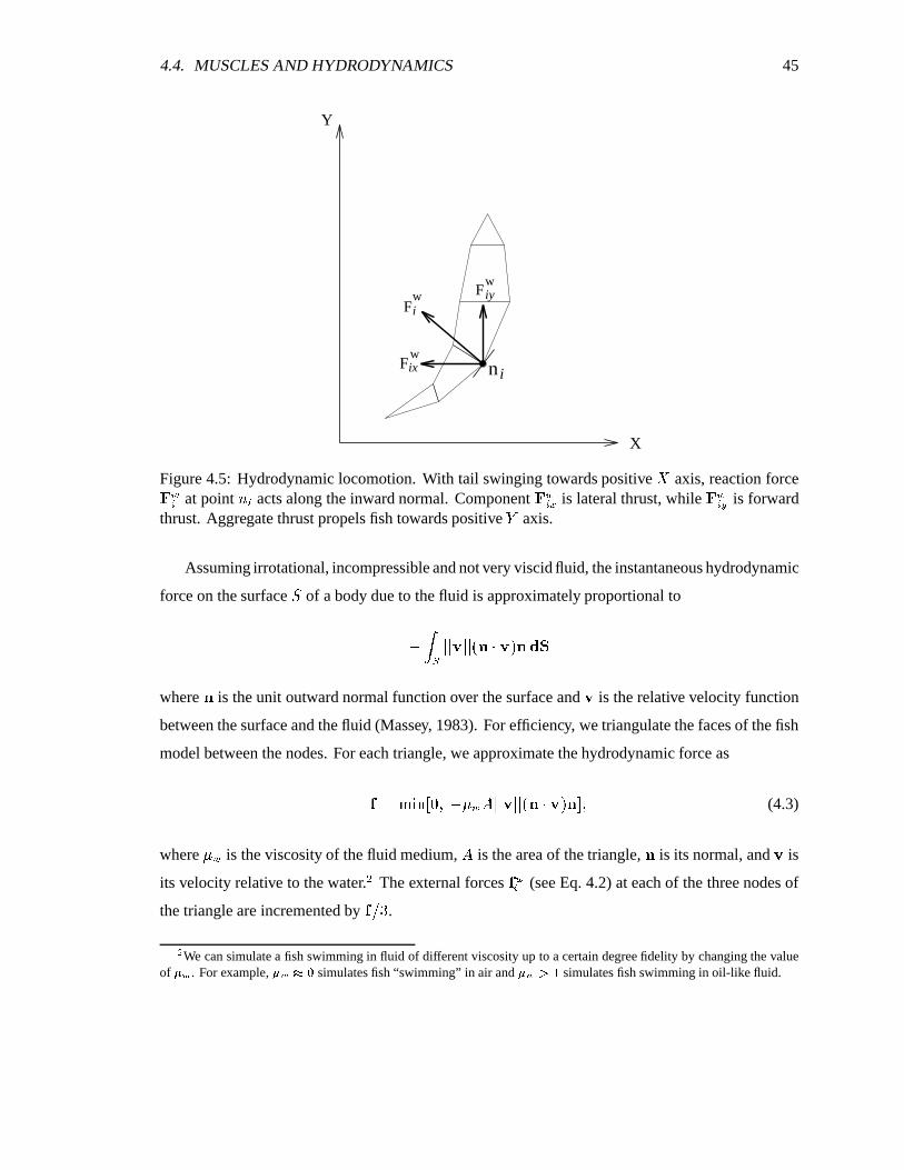
4.4. MUSCLES AND HYDRODYNAMICS 45
n i
F iyw
Fiw
Y
Fixw
X
Figure 4.5: Hydrodynamic locomotion. With tail swinging towards positive � axis, reaction force� Z� at point �w� acts along the inward normal. Component� Z��� is lateral thrust, while
� Z��� is forwardthrust. Aggregate thrust propels fish towards positive � axis.
Assuming irrotational, incompressible and not very viscid fluid, the instantaneous hydrodynamic
force on the surface - of a body due to the fluid is approximately proportional to
9g� R <5< ��<5<����YL������t� �where � is the unit outward normal function over the surface and � is the relative velocity function
between the surface and the fluid (Massey, 1983). For efficiency, we triangulate the faces of the fish
model between the nodes. For each triangle, we approximate the hydrodynamic force asC A�l������\���9�� Z�� <�< ��<�<����YL������K��� (4.3)
where � Z is the viscosity of the fluid medium, � is the area of the triangle, � is its normal, and � is
its velocity relative to the water. ) The external forcesC Z� (see Eq. 4.2) at each of the three nodes of
the triangle are incremented byC %&j .�
We can simulate a fish swimming in fluid of different viscosity up to a certain degree fidelity by changing the valueof #¡ . For example, #¡t¢�� simulates fish “swimming” in air and #¡l£�¤ simulates fish swimming in oil-like fluid.
46 CHAPTER 4. BIOMECHANICAL FISH MODEL AND LOCOMOTION
4.5 Numerical Solution
To simulate the dynamics of the fish model, the differential equations of motion (4.2) must be
integrated over time. The system is intrinsically stiff and can become unstable in a variety of
situations that may occur in the simulated dynamic world (e.g. executing a left turn to avoid a
sudden dynamic obstacle before completing a right turn). Therefore, the stability of the numerical
solution is an important consideration. We employ a simple, numerically stable, semi-implicit Euler
method.
The system of equations of motion Eq. (4.2) may be written in the standard matrix form for
nonlinear, damped elasto-dynamic systems (Bathe and Wilson, 1976) as follows:¥ W¦ ����SV§Y� ¦ � H¦ ����SV¨B� ¦ � ¦ ���© � ��� (4.4)
where¥
, § and ¨ are the mass, damping and stiffness matrices, respectively. Matrix¥
is
a constant diagonal matrix with � � on the main diagonal, while § and ¨ are time-dependent
nondiagonal matrices. These three matrices are of dimension ��ªe� where � is the number of nodes
in the biomechanical model. Matrices¦
, H¦ , W¦ consist of nodal position, velocity and acceleration
vectors, respectively, and�
is the matrix of external force vectors. These four matrices are of
dimension ��ªBj , such that each row contains the three components of each vector.
Because of the special properties of the viscoelastic units in our dynamic fish system, the damping
term §Y� ¦ � H¦ and the stiffness term ¨B� ¦ � ¦ in the above equation are most conveniently collected
into the form of an effective stiffness matrix «^� ¦ � H¦ � :«Y� ¦ � H¦ � ¦ ��� I§Y� ¦ � H¦ ���$S¬¨B� ¦ � ¦ ����
and hence Eq. (4.4) can be re-written as follows:¥ W¦ ����S«^� ¦ � H¦ � ¦ ��� � ��� (4.5)
where « is time-dependent since the viscoelastic forces depend nonlinearly on the nodal position
and velocity variables ������� and �������� .Our method computes the left-hand side of Eq. (4.5) implicitly and the right-hand side explicitly.
In particular, we discretize continuous time into time steps, \���®l�� FQF�F �����:SV®l�� FQF�F and solve for
4.5. NUMERICAL SOLUTION 47
H¦�¯�°�±w¯ in ¥ W¦ ¯�°�±w¯ S« ¯ ¦ ¯�°�±w¯ � ¯(4.6)
where represents simulation time and ®² is the simulation time step. We do not solve for the
position vectors¦�¯M°�±.¯
directly because, first, the velocity vectors H¦�¯ is readily available since it
has to be stored at each time step for computing « ¯ (more details can be found in the next section)
and, second, using H¦�¯ saves us from having to store¦�¯�³´±w¯
at each time step. We use the following
finite difference approximations for¦ ¯�°�±w¯
and W¦ ¯M°�±.¯ :¦ ¯�°�±w¯ ¦ ¯ S¬®l H¦ ¯�°�±w¯ (4.7)
and W¦ ¯M°�±.¯ i®² � H¦ ¯�°�±w¯ 9 H¦ ¯ � (4.8)
Substituting the above equations into Eq. (4.6) and collecting all known vectors on the right-hand
side, we obtain a linear system for H¦�¯�°�±w¯ :µ ¯ H¦ ¯�°�±w¯ u¶ ¯ (4.9)
where
µ ¯ z®lE« ¯ S ¥®² (4.10)
is the effective system matrix and
¶ ¯ � ¯ 9¬« ¯ ¦ ¯ S ¥®² H¦ ¯ (4.11)
is the effective load matrix. As we will explain in the next section, the structure the system matrix
µ ¯is such that an efficient solution to Eq. (4.9) can be obtained by assembling
µ ¯and factorizing
it as follows:
µ ¯ ¸·�¹�·»º»� (4.12)
where ¹ is diagonal and · is lower triangular. The new nodal velocities H¦ ¯�°�±w¯ are then computed
by first solving the lower triangular system
·�¼½ I¶ ¯ (4.13)
48 CHAPTER 4. BIOMECHANICAL FISH MODEL AND LOCOMOTION
for ¼ by forward-substitution and finally solving the upper triangular system
· º H¦ ¯�°�±w¯ "¹ ³ { ¼ (4.14)
for H¦ ¯M°�±.¯ by back-substitution. Hence, the numerical simulation of the fish biomechanical model
requires the assembly and factorization solution of a sequence of linear systems of the form of
Eq. 4.9 for � "\���®l���]#®l�� FQF�F .4.5.1 System Matrix Assembling and the Skyline Storage Scheme
Since the nodes of the dynamic fish model are not fully connected by viscoelastic units, the effective
stiffness matrix « ¯ and, consequently (since¥
is diagonal), the system matrix
µ ¯, are sparse
matrices. Sparsity can be exploited to increase the computational efficiency of the factorization
algorithms (Press et al., 1986). We have employed the Skyline Storage Scheme for storing
µ ¯, which
is popular in numerical methods for finite element analysis (Bathe and Wilson, 1976). This storage
scheme is most efficient for storing sparse matrices that are symmetric and banded. We will now
explain our strategy in more detail.
The �¾ª;� system matrix
µ ¯and �¾ª;j effective load matrix ¶ ¯ are computed according to
Eq. (4.10) and Eq. (4.11), respectively. To assemble
µ ¯, we first assemble the instantaneous, internal
effective viscoelastic stiffnesses T+�0/ of the system (see Eq. (4.1)). Denoting the entries of
µ ¯as ¿#�0/
and the rows of ¶ ¯ as Àw� , the following procedure assembles
µ ¯and ¶ ¯ :
1. Initialize
µ ¯ "Á and ¶ ¯ "Á .
2. For each viscoelastic unit -.�0/ , assemble the ®lE« ¯ term of Eq. (4.10) into
µ ¯:
¿#���$ "¿#���wST+�0/�®l¿Q/�/y "¿�//�S¬T+�0/�®l¿#�0/y "¿�/��$ �9�T+�0/�®land assemble the 9�« ¯ ¦ ¯ term of Eq. (4.11) into ¶ :
À � AÀ � ST �0/ > � /À*/y OÀÂ/�9;T+�0/�>Q�0/
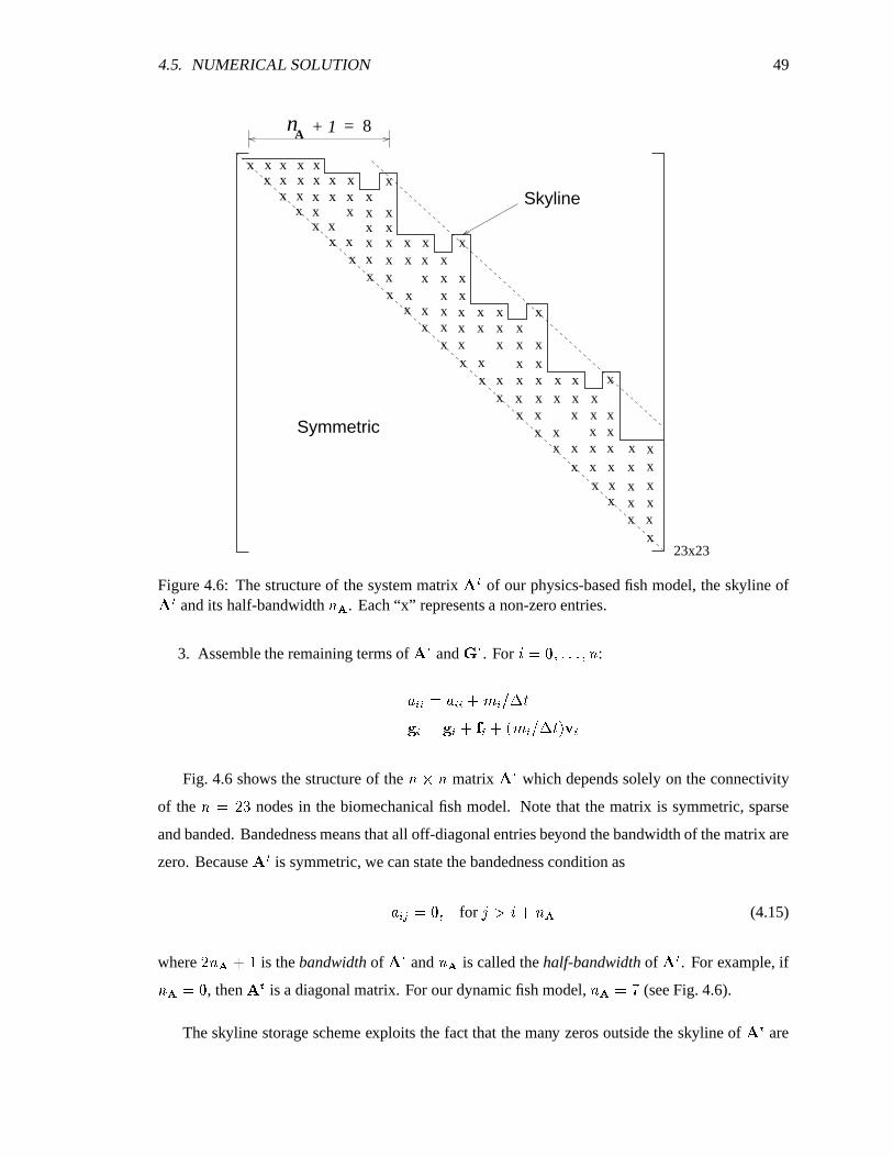
4.5. NUMERICAL SOLUTION 49
= 8
Skyline
x
xx
xx
xx
x
xx
x
xx
x
xx
xx
xx
xx x x x x x
x x x xxx x x
x x xx x x x x x
x x x x xx x
x x xx
A
x x x xxx x x x x
x x xx x
x x x x xx x x x x
x x xx x
x x x xx x x
x xxx
xxx
xx
x
x
x
x
x
x
Symmetric
23x23
+ 1n
x
x
x
xx
x x
Figure 4.6: The structure of the system matrix
µ ¯of our physics-based fish model, the skyline of
µ ¯and its half-bandwidth �wà . Each “x” represents a non-zero entries.
3. Assemble the remaining terms of
µ ¯and ¶ ¯ . For
� "\�� FQFQF ��� :
¿#���© "¿'����S����%+®lÀ.�© OÀw�.S C �.SA�E����%&®l�����Fig. 4.6 shows the structure of the �;ªB� matrix
µ ¯which depends solely on the connectivity
of the �¸ Ä]#j nodes in the biomechanical fish model. Note that the matrix is symmetric, sparse
and banded. Bandedness means that all off-diagonal entries beyond the bandwidth of the matrix are
zero. Because
µ ¯is symmetric, we can state the bandedness condition as
¿'� /y z\�� for 1eÅ � S¬�wà (4.15)
where ]#� Ã Szi is the bandwidth of
µ ¯and � Ã is called the half-bandwidth of
µ ¯. For example, if�wÃV "\ , then
µ ¯is a diagonal matrix. For our dynamic fish model, �wÃV IÆ (see Fig. 4.6).
The skyline storage scheme exploits the fact that the many zeros outside the skyline of
µ ¯are

50 CHAPTER 4. BIOMECHANICAL FISH MODEL AND LOCOMOTION
unnecessary in the factorization solution of Eq. 4.9. Hence, an effective way of storing the symmetric
µ ¯would be to store only the upper triangular half of the matrix below the skyline, including the
diagonal. Ç The skyline storage scheme stores
µ ¯into a one-dimensional array È� . In addition, it
uses an auxiliary array to properly address the entries of
µ ¯stored in È� .
We explain the matrix storage and addressing scheme via a small example system matrix
µof
order 4 shown in Fig. 4.7. Let �.� be the row number of the first nonzero entry in column�
of
µ.
The variables �w� , � z\��Qi#��]�� F�F5F , define the skyline of the matrix and � � 9B�w�� are the column heights.
Furthermore, the half-bandwidth of the matrix, �wà , equals ��É�Ê´��� � 9¾�.��� . With the column heights
defined, we can now store all entries of
µbelow its skyline consecutively in È� . Fig. 4.7 shows how
the entries of
µare stored in È� . In addition to È� , we also define an array MAX È� , which stores the
indexes of the diagonal entries of
µ, ¿#��� , in È� . Note that MAX È� � � � is equal to the sum of column
heights up to the � � 9zi+� th column plus�. Hence, the number of stored entries in the
�th column
of
µis equal to MAX È� � � SËiU��9 MAX È� � � � and the entry indexes are MAX È� � � � , MAX È� � � � SËi ,
MAX È� � � �$S¬] , ..., MAX È� � � SOi+�©9Vi . Therefore, storing
µin the form of È� and MAX È� allows the
entries of
µto be easily addressed.
a
aa
a
MAXA =
021211 22
02
a
33
2322
1211
34
a
a
a
a
44
33
aaaa a
aA =
aaaa
a a344423aa a a a a
A =
7654 81 3
10
00
2
20
00
75
n2
Symmetric
= 23n
= 0
Figure 4.7: An example of the skyline storage scheme. � is the example system matrix; È� is thestorage array and MAX È� is the index array.Ì
Note that zero entries within this region will need to be stored because they can become nonzero during calculations.
4.5. NUMERICAL SOLUTION 51
A factorization solution of Eq. 4.9 using skyline storage is substantially more efficient compared
to a Gaussian elimination solution which has Ͳ�E� Ç � complexity in terms of the number of operations
required (an operation is defined as a multiplication and an addition), where � is the order of
µ ¯. For
factorization with skyline storage, the number of operations required is Ͳ�E�N� )à � in the worst case
of constant column heights (i.e.� 9¬�w�© "�wà for all
�). Clearly, the larger the difference between �
and � à , the greater the advantage. In simulating the dynamics of the artificial fish, we have �� "]#jand �wÃA �Æ which represents a significant improvement in computational efficiency. Note that the
column heights� 9¬�w� of a system matrix
µ ¯and, hence, the effectiveness of the storage scheme,
depends on how the nodes in the discrete dynamic model are numbered. For example, using our
current numbering scheme, �wÃO cÆ (Fig. 4.6), however if we number node 22 as node 1 (referring
to Fig. 4.2), �wÃÎ Ï�B9Ii� Ï]#] . Thus in general, one should number the nodes in such a way
that all connections are as local as possible. We can frequently determine a reasonable nodal point
numbering by inspection. However, this numbering may not be particularly easy to generate in
certain cases (Bathe and Wilson, 1976). Ð4.5.2 Algorithm Outline and Discussion
An outline of our semi-implicit simulation algorithm is as follows:
Initial calculations at � "\ :1. Initialize
¦ v , H¦ v and W¦ v .2. From the connectivity of the mass-spring-damper model, initialize the skyline storage scheme:
Calculate the dimension of � from column heights and the index array MAX � .
For each time step � "®l���]#®²�� F�FQF :1. Calculate the system matrix
µ ¯and the effective load matrix ¶ ¯ as prescribed in Section 4.5.1.
2. Factorize
µ ¯ "·�¹�· º , where ¹ is diagonal and · is lower triangular.ÑThe symmetry and bandedness properties of the system matrix associated with the mass-spring-damper fish model
would carry over to other mass-spring models (Miller, 1988; Terzopoulos and Waters, 1990; Grzeszczuk and Terzopoulos,1995; Lee, Terzopoulos and Waters, 1995). Hence, the skyline storage scheme is generally applicable to these modelsto improve computational efficiency. Note, however, that all of these prior models used simple, explicit time integrationmethods which do not involve matrix assembly and factorization. As we stated earlier, explicit methods are inadequate tosimulate the dynamics of the fish biomechanical model because of their limited stability.
52 CHAPTER 4. BIOMECHANICAL FISH MODEL AND LOCOMOTION
3. Solve for the new velocities H¦�¯�°�±w¯ :(a) Solve ·�¼Ä u¶ ¯ for ¼ using forward-substitution.
(b) Solve · º H¦ ¯M°�±.¯ Ò¹ ³ { ¼ for H¦ ¯�°�±w¯ using back-substitution. Note that since ¹ is
diagonal, the computation of its inverse ¹ ³ { is trivial.
4. Update the nodal positions:¦ ¯�°�±w¯ H¦ ¯�°�±w¯ ®l©S ¦ ¯ .
We have verified experimentally that the semi-implicit algorithm is sufficiently stable for our
simulation purposes. We use a time step of ®l� ¸\ F \ p#p in our simulator (the stability limit is reached
with a time step around ®l�ÓI\ F i ). Our algorithm is much more stable than an explicit Euler time
integration implementation. Given the same numerical settings, experiments show that the largest
time step allowed (before the system becomes unstable) when using our algorithm is typically iQ\#\ toi p \ times larger than is possible when using the explicit method. On the other hand, our algorithm
is simpler than implicit methods described by Bathe and Wilson (1976), such as the Houbolt method
or the Newmark method. In particular, the approximations we use for¦ ¯�°�±w¯
(Eq. 4.7) and W¦ ¯M°�±.¯(Eq. 4.8) are simple and require only knowledge of the position matrix
¦ ¯and the velocity matrixH¦ ¯ at time while other methods (for example the Houbolt method) requires positions and velocities
from several previous time steps. Furthermore, fully implicit methods require that the external load
matrix� ¯
in Eq. (4.6) be calculated implicitly as well, which would be difficult in our case.
4.6 Motor Controllers
We have described the structure, mechanics, hydrodynamics and the numerical simulation of the
physics-based fish model. In this section, we proceed to describe how we implement the repertoire
of biomechanics-based motor skills of the artificial fish.
A critical first step towards higher level, behavioral modeling is to abstract, as a set of motor
controllers, the detailed muscle actions, and pectoral fin motions required for locomotion. These
motor controllers serve as the behavioral building blocks. They are implemented as parameterized
procedures, hence allowing the easy expression of behaviors. In particular, behaviors, as elaborate as
the mating behavior, emerge from the invocation of a sequence of motor controllers with appropriate
parameters in a meaningful order.
Currently the repertoire of motor skills of the artificial fish is implemented by nine motor
4.6. MOTOR CONTROLLERS 53
controllers:
1. Ô&ÕNÖ�×$Ø+Ù´Ú2. Û�Ü+Ý*ÞwØ+Þ#ß�à#áNØ+Ù´Ú3. àKÖ�â#ã�ÞwØ&Þ'ß´à'áNØ&Ù�Ú4. â´ÛwÖ&äxÜÂØ&Ù�Ú5. å*ÔÂæ*Ü�á.ä�Ø+Ù´Ú6. ä�ÜÂÔ*æÂÜ�áxäxØ&Ù�Ú7. çKå#Û�å�áNæ*ÜÂØ&Ù�Ú8. ç´àwå&èwÜÂØ&Ù�Ú9. çKå#Û�å�áNæ*ÜÂØ&Ù�ÚEach motor controller carries out a specific motor function. Four of the motor controllers
prescribe the muscle contractions of the biomechanical fish model: Ô+ÕNÖ�×$Ø&Ù�Ú produces forward
caudal locomotion, ÛxÜ+Ý*ÞwØ&Þ'ß�à#áNØ&Ù�Ú and àKÖ�â'ã´ÞwØ&Þ'ß�à#áNØ&Ù�Ú execute turns, while â�Û.Ö+ä�ÜÂØ+Ù´Ú allows
gliding and smooth transitions from forward swimming to turning and vise versa. The other five
motor controllers control the fish’s pectoral fins that enable it to navigate freely in its 3D virtual
world: åÂÔ*æÂÜQá.äxØ&Ù�Ú produces lift, ä�ÜÂÔ*æÂÜ�áxäxØ&Ù�Ú controls diving, çKå#ÛxåQáNæ*ÜÂØ+Ù´Ú enables the fish to
maintain its balance, ç´àwå&èwÜÂØ&Ù�Ú slows the forward velocity, and çNå*æ+èÂÕ.å+à´äxØ+Ù´Ú allows the fish to
retreat.
In the following sections,we explain the implementation of the muscle motor controllers followed
by the pectoral fin motor controllers.
4.6.1 Muscle Motor Controllers
Muscle motor controllers implement the designated motor functions by controlling the contractions
of the twelve muscles. é According to Webb (1989), given the length of the fish body, the swimming
speed of most fishes below certain threshold values is roughly proportional to the amplitude and
frequency of the periodic lateral oscillations of the tail. Our experiments with the mechanical model
agree well with these observations. Both the swimming speed and the turn angle of the fish model
are approximately proportional to the contraction amplitudes and frequencies/rates of the muscles.êThe swimming motor controller controls the swimming segment muscles (see Fig. 4.2), while the turning motor
controllers control the turning segment muscles.
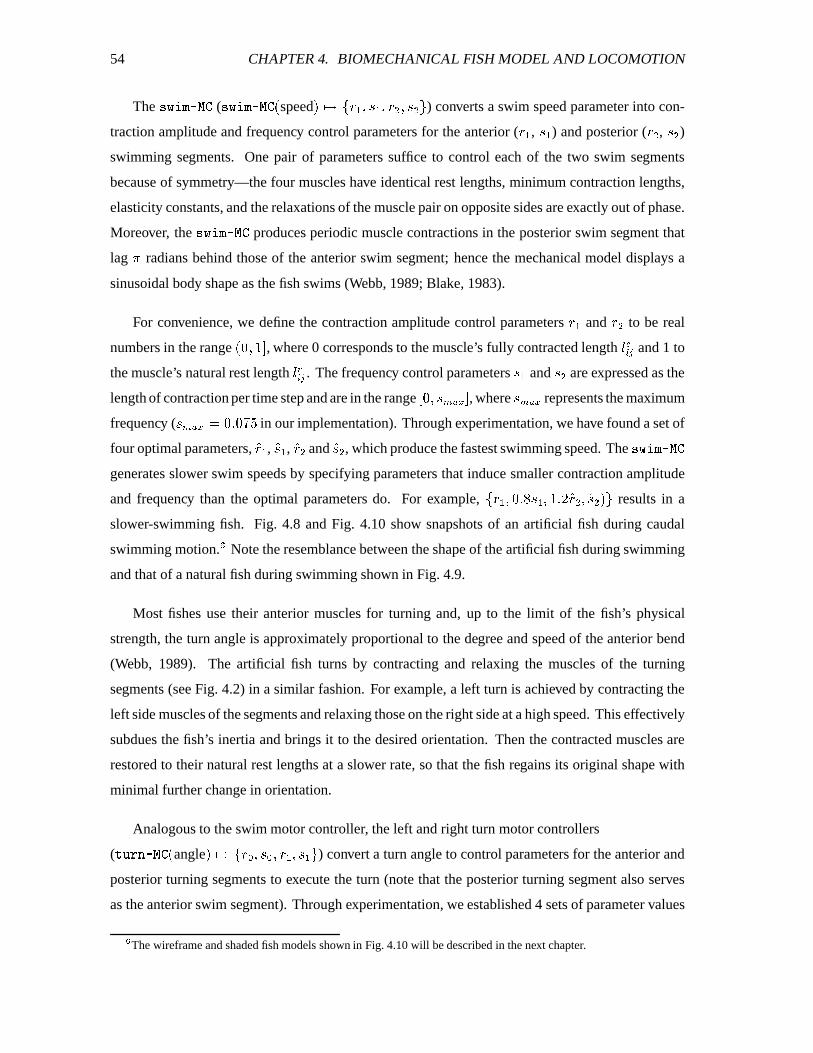
54 CHAPTER 4. BIOMECHANICAL FISH MODEL AND LOCOMOTION
The Ô&ÕNÖ�×$Ø+Ù´Ú ( Ô+ÕKÖ�×$Ø&Ù�ÚÂ� speed ��ëìîí&8 { ��ï { ��8 ) ��ï )?ð ) converts a swim speed parameter into con-
traction amplitude and frequency control parameters for the anterior ( 8 { , ï { ) and posterior ( 8 ) , ï ) )swimming segments. One pair of parameters suffice to control each of the two swim segments
because of symmetry—the four muscles have identical rest lengths, minimum contraction lengths,
elasticity constants, and the relaxations of the muscle pair on opposite sides are exactly out of phase.
Moreover, the Ô&ÕNÖ�×$Ø+Ù´Ú produces periodic muscle contractions in the posterior swim segment that
lag ñ radians behind those of the anterior swim segment; hence the mechanical model displays a
sinusoidal body shape as the fish swims (Webb, 1989; Blake, 1983).
For convenience, we define the contraction amplitude control parameters 8 { and 8 ) to be real
numbers in the range �E\���i�� , where 0 corresponds to the muscle’s fully contracted length 4�ò�0/ and 1 to
the muscle’s natural rest length 4Mó�0/ . The frequency control parameters ï { and ï ) are expressed as the
length of contraction per time step and are in the range ��\���ï7ôöõ,��� , where ï7ôöõ,� represents the maximum
frequency ( ï7ôöõ÷�l "\ F \ÂÆ p in our implementation). Through experimentation, we have found a set of
four optimal parameters, ø8 { , øï { , ø8 ) and øï ) , which produce the fastest swimming speed. The Ô+ÕKÖ�×$Ø&Ù�Úgenerates slower swim speeds by specifying parameters that induce smaller contraction amplitude
and frequency than the optimal parameters do. For example, í�ø8 { ��\ F q©øï { ��i F ]©ø8 ) �*øï ) � ð results in a
slower-swimming fish. Fig. 4.8 and Fig. 4.10 show snapshots of an artificial fish during caudal
swimming motion. ù Note the resemblance between the shape of the artificial fish during swimming
and that of a natural fish during swimming shown in Fig. 4.9.
Most fishes use their anterior muscles for turning and, up to the limit of the fish’s physical
strength, the turn angle is approximately proportional to the degree and speed of the anterior bend
(Webb, 1989). The artificial fish turns by contracting and relaxing the muscles of the turning
segments (see Fig. 4.2) in a similar fashion. For example, a left turn is achieved by contracting the
left side muscles of the segments and relaxing those on the right side at a high speed. This effectively
subdues the fish’s inertia and brings it to the desired orientation. Then the contracted muscles are
restored to their natural rest lengths at a slower rate, so that the fish regains its original shape with
minimal further change in orientation.
Analogous to the swim motor controller, the left and right turn motor controllers
( Þ'ß´à'áKØ+Ù�ÚÂ� angle ��ëìúí&8�v���ïQv���8 { ��ï { ð ) convert a turn angle to control parameters for the anterior and
posterior turning segments to execute the turn (note that the posterior turning segment also serves
as the anterior swim segment). Through experimentation, we established 4 sets of parameter valuesûThe wireframe and shaded fish models shown in Fig. 4.10 will be described in the next chapter.
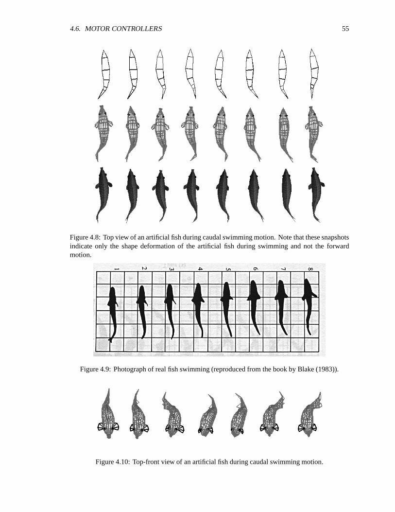
4.6. MOTOR CONTROLLERS 55
Figure 4.8: Top view of an artificial fish during caudal swimming motion. Note that these snapshotsindicate only the shape deformation of the artificial fish during swimming and not the forwardmotion.
Figure 4.9: Photograph of real fish swimming (reproduced from the book by Blake (1983)).
Figure 4.10: Top-front view of an artificial fish during caudal swimming motion.
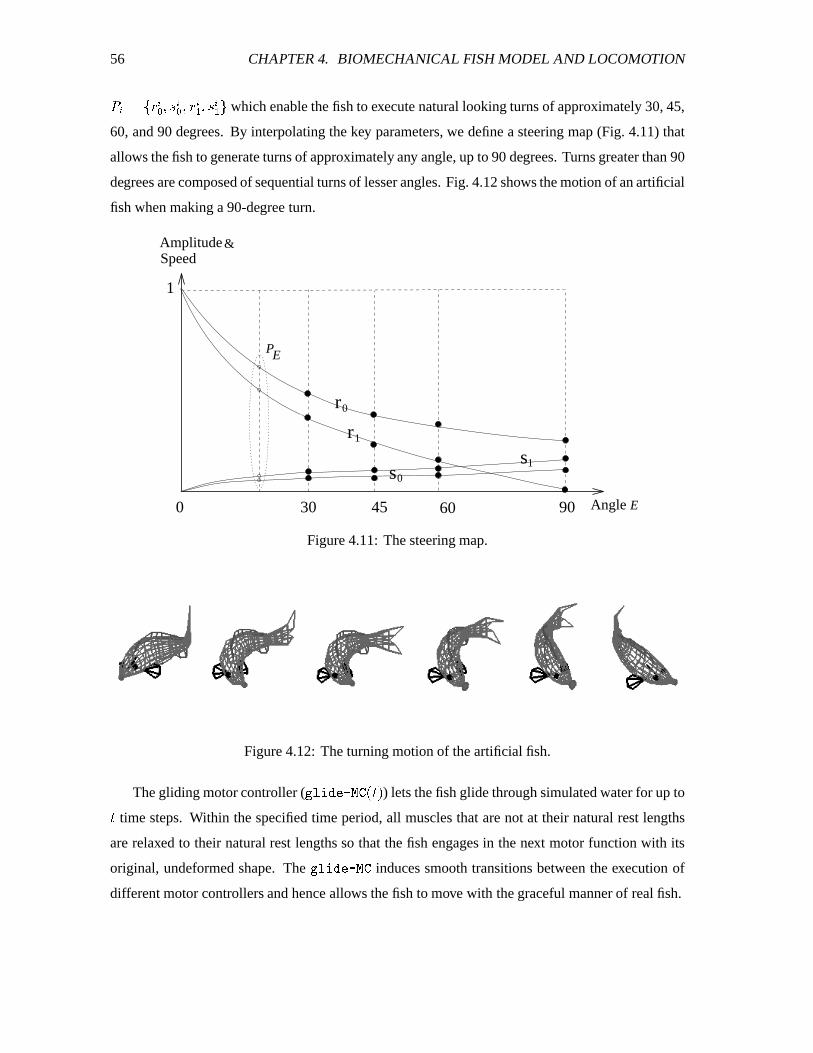
56 CHAPTER 4. BIOMECHANICAL FISH MODEL AND LOCOMOTIONü � uí&8 �v ��ï � v ��8 � { ��ï � { ð which enable the fish to execute natural looking turns of approximately 30, 45,
60, and 90 degrees. By interpolating the key parameters, we define a steering map (Fig. 4.11) that
allows the fish to generate turns of approximately any angle, up to 90 degrees. Turns greater than 90
degrees are composed of sequential turns of lesser angles. Fig. 4.12 shows the motion of an artificial
fish when making a 90-degree turn.
0
s0
s1
r1
r
&
0
AmplitudeSpeed
1
30 45 60 90 Angle
PE
E
Figure 4.11: The steering map.
Figure 4.12: The turning motion of the artificial fish.
The gliding motor controller ( â�ÛwÖ&äxÜ*Ø+Ù�Ú���� ) lets the fish glide through simulated water for up to time steps. Within the specified time period, all muscles that are not at their natural rest lengths
are relaxed to their natural rest lengths so that the fish engages in the next motor function with its
original, undeformed shape. The â´ÛwÖ+ä�ÜÂØ&Ù�Ú induces smooth transitions between the execution of
different motor controllers and hence allows the fish to move with the graceful manner of real fish.
4.6. MOTOR CONTROLLERS 57
4.6.2 Pectoral Fin Motor Controllers
The pectoral fins on most fish control pitching (up-and-down motion of the body), yawing (the
side-to-side motion) and rolling. The pectoral fins can be held close to the body to increase speed
by reducing drag, or they can be extended to increase drag and serve as a brake (Wilson and
Wilson, 1985). Many reef fishes use pectoral swimming to achieve very fine motion control, such
as backwards motions, by keeping their bodies still and using their pectoral fins like oars. Through
functional modeling, we successfully synthesize a full range of pectoral motor control in artificial
fishes.
To model the pectoral fins, we equip the artificial fish with five additional parameterized motor
skills, namely, the åÂÔ*æÂÜ�áxäxØ&Ù�Ú , äxÜ*ÔÂæÂÜQá.ä�Ø+Ù�Ú , çNå#Û�å�áKæÂÜÂØ&Ù�Ú , ç´àwå&èwÜÂØ&Ù�Ú and çKåÂæ+è*Õwå&à�äxØ&Ù�Ú . The
artificial fish is neutrally buoyant in the virtual water and the pair of pectoral fins enable it to
navigate freely in its 3D world. The pectoral fins function in a similar, albeit simplified, manner to
those of real fishes. For our purposes, the detailed movement of the pectoral fins is of less interest
than the movement of the fish body. To simplify the fish model and its numerical solution, we do not
simulate the elasticity and dynamics of the pectoral fins. However, we do approximate the dynamic
forces that the pectoral fins exert on the body of the fish to control locomotion.
g
v
n
vγ
γ
fin orientation
fish orientation
Figure 4.13: The pectoral fin geometry.
The pectoral fins (Fig. 4.13) work by applying reaction forces to nodes in the midsection of the
fish body, i.e. nodes fh�,�Qi�k � k½iQ] (see Fig. 4.2). The fins are analogous to the airfoils of an
airplane. Pitch and yaw control stems from changing their orientations ñ©%�nYkVýþkAñ relative to the
body. Assuming that a fin has an area � , surface normal � and the fish has a velocity � relative to
the water (Fig. 4.13), the fin force isÿ�� �9 � <5< ��<5<�����L������� �9µ�?<5< ��<5< ������� ý©��� (4.16)
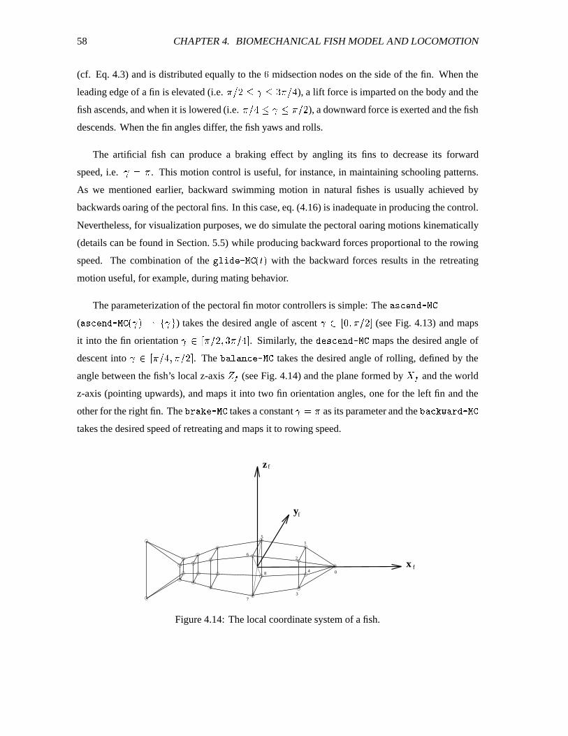
58 CHAPTER 4. BIOMECHANICAL FISH MODEL AND LOCOMOTION
(cf. Eq. 4.3) and is distributed equally to the o midsection nodes on the side of the fin. When the
leading edge of a fin is elevated (i.e. ñ©%&]lkVý�kOj#ñ©%Qn ), a lift force is imparted on the body and the
fish ascends, and when it is lowered (i.e. ñ©%�nYkVýþkAñ©%&] ), a downward force is exerted and the fish
descends. When the fin angles differ, the fish yaws and rolls.
The artificial fish can produce a braking effect by angling its fins to decrease its forward
speed, i.e. ýV =ñ . This motion control is useful, for instance, in maintaining schooling patterns.
As we mentioned earlier, backward swimming motion in natural fishes is usually achieved by
backwards oaring of the pectoral fins. In this case, eq. (4.16) is inadequate in producing the control.
Nevertheless, for visualization purposes, we do simulate the pectoral oaring motions kinematically
(details can be found in Section. 5.5) while producing backward forces proportional to the rowing
speed. The combination of the â�ÛwÖ&äxÜ*Ø+Ù�Ú#���� with the backward forces results in the retreating
motion useful, for example, during mating behavior.
The parameterization of the pectoral fin motor controllers is simple: The å*ÔÂæÂÜQá.ä�Ø+Ù�Ú( åÂÔ*æÂÜQá.äxØ&Ù�ÚÂ� Èý$�Pëì íQý ð ) takes the desired angle of ascent ÈýOdI��\x��ñ©%&]U� (see Fig. 4.13) and maps
it into the fin orientation ýOdz��ñö%&]���j'ñ©%�n#� . Similarly, the äxÜÂÔ*æÂÜQá.äxØ&Ù�Ú maps the desired angle of
descent into ýOdI��ñö%Qn.��ñö%&]+� . The çNåUÛxå�áKæÂÜ*Ø+Ù�Ú takes the desired angle of rolling, defined by the
angle between the fish’s local z-axis � (see Fig. 4.14) and the plane formed by � � and the world
z-axis (pointing upwards), and maps it into two fin orientation angles, one for the left fin and the
other for the right fin. The ç´àwå&èwÜÂØ&Ù�Ú takes a constant ýg "ñ as its parameter and the çNå*æ+èÂÕ.å+à´äxØ+Ù´Útakes the desired speed of retreating and maps it to rowing speed.
0
1
2
3
6
7
8 4
5
fz
fy
fx
Figure 4.14: The local coordinate system of a fish.
Chapter 5
Modeling the Form and Appearance of
Fishes
To achieve realistic computer animation, our artificial fish model must capture the form and appear-
ance of real fishes with adequate fidelity. In this chapter we design texture mapped, 3D geometric
display models with which to “envelope” the biomechanical fish model described in Chapter 4, thus
constructing different artificial fishes. We begin with color photographs of real fishes and build
free-form geometric models of several different species using nonuniform rational B-spline (NURBS)
surfaces. We develop a new interactive tool for segmenting portions of the fish images to be used
as texture maps that are subsequently rendered onto the geometric display surfaces. Finally, we de-
scribe how this geometric display model is coupled to the dynamic model of the fish to appropriately
actuate and deform the display model. We also describe the visualization of the pectoral fin motion
in the display model.
5.1 Constructing 3D Geometric Fish Models
The geometric fish models are constructed manually using the AliasTM 3D modeler. We model the
shape of any given fish’s body in accordance with the shape evident in digitized color pictures of the
animal (Fig. 5.1). We employ two juxtaposed NURBS surfaces, one for the left half and the other for
the right half of the fish body. The NURBS surfaces are of order j (or of degree 4) along both the Jand � axes ( J and � represent the two axes of the material coordinates of a surface). Each NURBS
surface has �ª�� control points which, when connected, form a surface mesh as shown in Fig. 5.2.
59
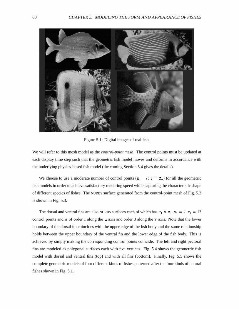
60 CHAPTER 5. MODELING THE FORM AND APPEARANCE OF FISHES
Figure 5.1: Digital images of real fish.
We will refer to this mesh model as the control-point mesh. The control points must be updated at
each display time step such that the geometric fish model moves and deforms in accordance with
the underlying physics-based fish model (the coming Section 5.4 gives the details).
We choose to use a moderate number of control points ( ¾ Ëm ; �� ]�i ) for all the geometric
fish models in order to achieve satisfactory rendering speed while capturing the characteristic shape
of different species of fishes. The NURBS surface generated from the control-point mesh of Fig. 5.2
is shown in Fig. 5.3.
The dorsal and ventral fins are also NURBS surfaces each of which has { ª�� { , { "]���� { �iQ]control points and is of order 1 along the J axis and order 3 along the � axis. Note that the lower
boundary of the dorsal fin coincides with the upper edge of the fish body and the same relationship
holds between the upper boundary of the ventral fin and the lower edge of the fish body. This is
achieved by simply making the corresponding control points coincide. The left and right pectoral
fins are modeled as polygonal surfaces each with five vertices. Fig. 5.4 shows the geometric fish
model with dorsal and ventral fins (top) and with all fins (bottom). Finally, Fig. 5.5 shows the
complete geometric models of four different kinds of fishes patterned after the four kinds of natural
fishes shown in Fig. 5.1.
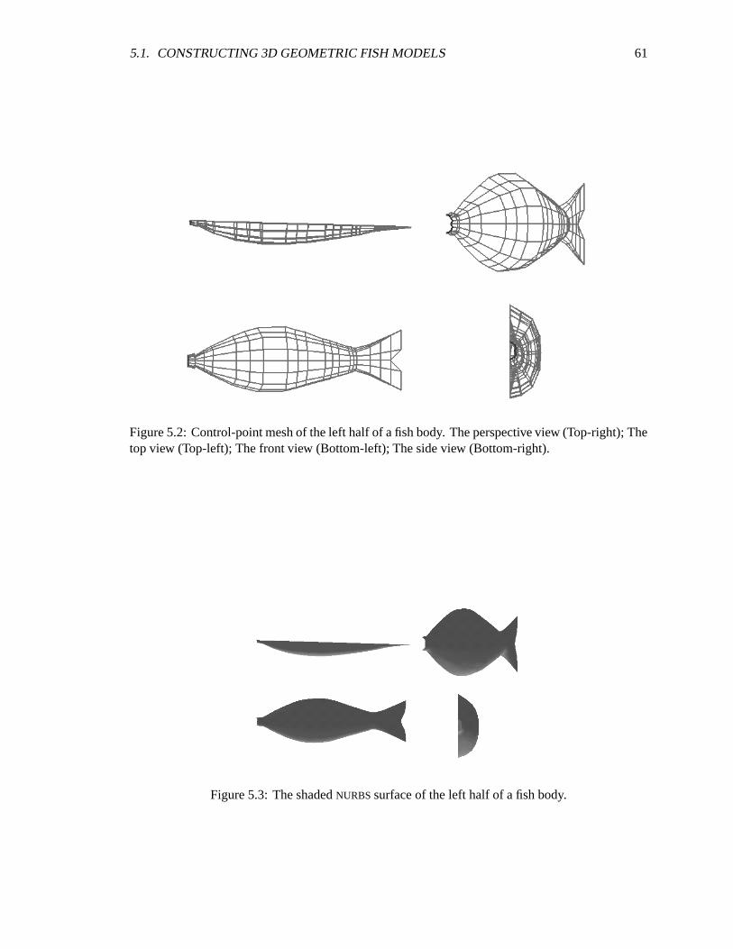
5.1. CONSTRUCTING 3D GEOMETRIC FISH MODELS 61
Figure 5.2: Control-point mesh of the left half of a fish body. The perspective view (Top-right); Thetop view (Top-left); The front view (Bottom-left); The side view (Bottom-right).
Figure 5.3: The shaded NURBS surface of the left half of a fish body.
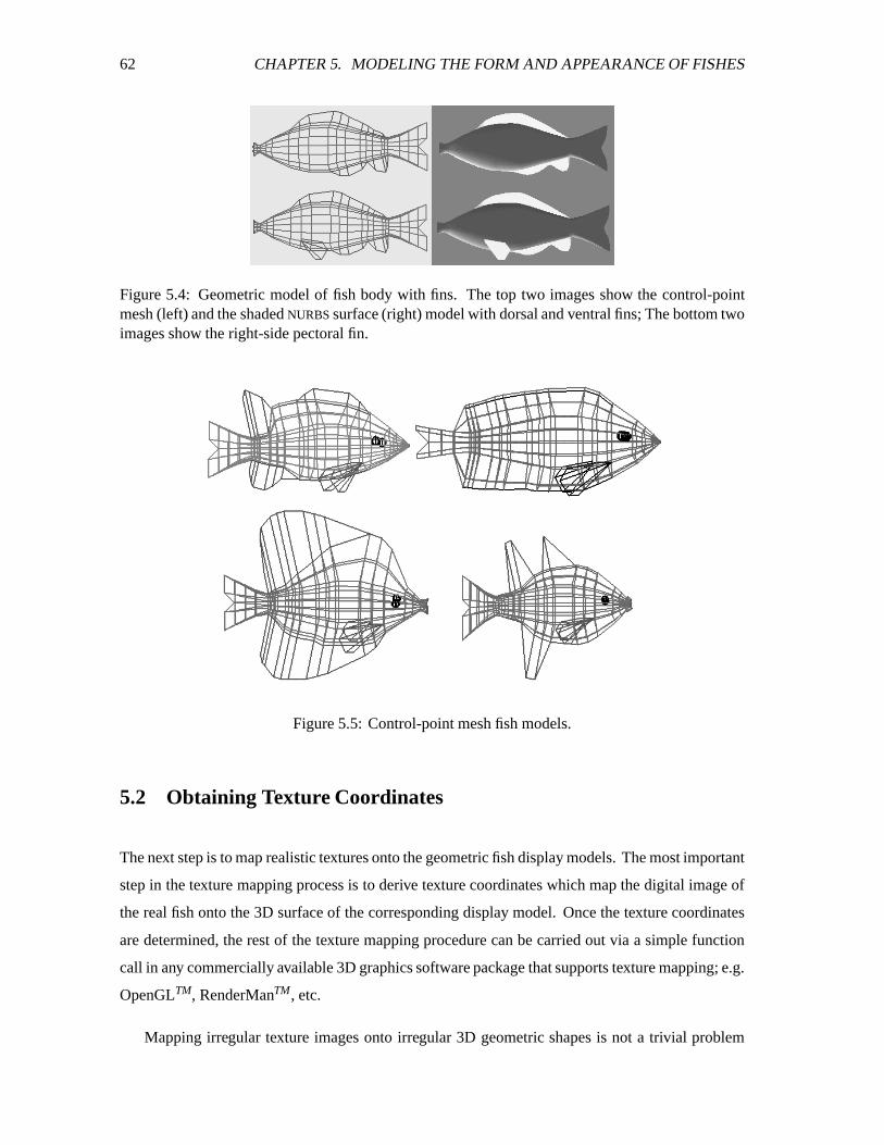
62 CHAPTER 5. MODELING THE FORM AND APPEARANCE OF FISHES
Figure 5.4: Geometric model of fish body with fins. The top two images show the control-pointmesh (left) and the shaded NURBS surface (right) model with dorsal and ventral fins; The bottom twoimages show the right-side pectoral fin.
Figure 5.5: Control-point mesh fish models.
5.2 Obtaining Texture Coordinates
The next step is to map realistic textures onto the geometric fish display models. The most important
step in the texture mapping process is to derive texture coordinates which map the digital image of
the real fish onto the 3D surface of the corresponding display model. Once the texture coordinates
are determined, the rest of the texture mapping procedure can be carried out via a simple function
call in any commercially available 3D graphics software package that supports texture mapping; e.g.
OpenGLTM, RenderManTM, etc.
Mapping irregular texture images onto irregular 3D geometric shapes is not a trivial problem
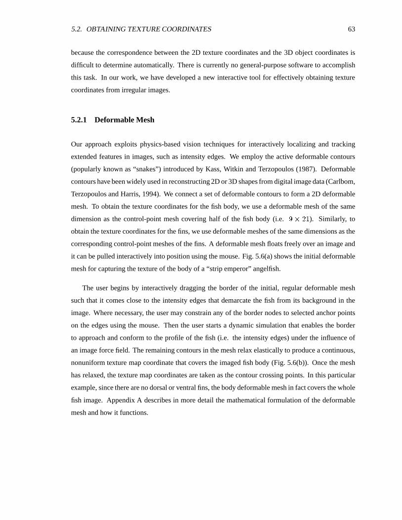
5.2. OBTAINING TEXTURE COORDINATES 63
because the correspondence between the 2D texture coordinates and the 3D object coordinates is
difficult to determine automatically. There is currently no general-purpose software to accomplish
this task. In our work, we have developed a new interactive tool for effectively obtaining texture
coordinates from irregular images.
5.2.1 Deformable Mesh
Our approach exploits physics-based vision techniques for interactively localizing and tracking
extended features in images, such as intensity edges. We employ the active deformable contours
(popularly known as “snakes”) introduced by Kass, Witkin and Terzopoulos (1987). Deformable
contours have been widely used in reconstructing 2D or 3D shapes from digital image data (Carlbom,
Terzopoulos and Harris, 1994). We connect a set of deformable contours to form a 2D deformable
mesh. To obtain the texture coordinates for the fish body, we use a deformable mesh of the same
dimension as the control-point mesh covering half of the fish body (i.e. m�ªV]�i ). Similarly, to
obtain the texture coordinates for the fins, we use deformable meshes of the same dimensions as the
corresponding control-point meshes of the fins. A deformable mesh floats freely over an image and
it can be pulled interactively into position using the mouse. Fig. 5.6(a) shows the initial deformable
mesh for capturing the texture of the body of a “strip emperor” angelfish.
The user begins by interactively dragging the border of the initial, regular deformable mesh
such that it comes close to the intensity edges that demarcate the fish from its background in the
image. Where necessary, the user may constrain any of the border nodes to selected anchor points
on the edges using the mouse. Then the user starts a dynamic simulation that enables the border
to approach and conform to the profile of the fish (i.e. the intensity edges) under the influence of
an image force field. The remaining contours in the mesh relax elastically to produce a continuous,
nonuniform texture map coordinate that covers the imaged fish body (Fig. 5.6(b)). Once the mesh
has relaxed, the texture map coordinates are taken as the contour crossing points. In this particular
example, since there are no dorsal or ventral fins, the body deformable mesh in fact covers the whole
fish image. Appendix A describes in more detail the mathematical formulation of the deformable
mesh and how it functions.
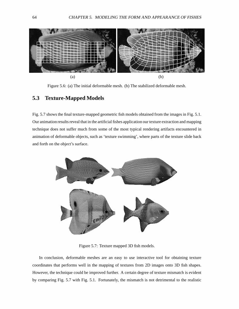
64 CHAPTER 5. MODELING THE FORM AND APPEARANCE OF FISHES
(a) (b)
Figure 5.6: (a) The initial deformable mesh. (b) The stabilized deformable mesh.
5.3 Texture-Mapped Models
Fig. 5.7 shows the final texture-mapped geometric fish models obtained from the images in Fig. 5.1.
Our animation results reveal that in the artificial fishes application our texture extraction and mapping
technique does not suffer much from some of the most typical rendering artifacts encountered in
animation of deformable objects, such as ‘texture swimming’, where parts of the texture slide back
and forth on the object’s surface.
Figure 5.7: Texture mapped 3D fish models.
In conclusion, deformable meshes are an easy to use interactive tool for obtaining texture
coordinates that performs well in the mapping of textures from 2D images onto 3D fish shapes.
However, the technique could be improved further. A certain degree of texture mismatch is evident
by comparing Fig. 5.7 with Fig. 5.1. Fortunately, the mismatch is not detrimental to the realistic
5.4. COUPLING THE DYNAMIC AND DISPLAY MODELS 65
appearance of the fishes on the whole. Note that the mismatch is largely due to the fact that the 3D
geometric models do not accurately resemble the original fish outline while the deformable mesh
does. The problem arises because the process of generating the 3D geometric models is for now
separate from that of generating the texture coordinates. With additional work, it should be possible
to unify the process of defining the contour control points for the NURBS surfaces with the texture
contour generation process.
Another observation is that although texture mapping using scanned digital images leads to
photo-realistic appearance, it has several limitations. First, if we want to render a large school of
fish of the same species, each with slightly different textures, we would have to store as many digital
images as there are fish. Second, many animals, including fishes, may change their colorations
during a particular period of time for behavioral purposes. For example, most male fish are able to
grow exceptionally colorful textures during mating seasons to attract female fish. Chameleons have
the ability to change their colors according the color of the immediate environment to camouflage
themselves. Yet others may change their colors according their moods. Hence, it may be useful to
model the variation of colors and textures across different animals (in the same species) or for any
individual animal over time. However it is inconvenient to capture, scan, and segment all the natural
images necessary to do so. An alternative approach would be to modify a single captured texture
procedurally or to generate purely synthetic textures procedurally. The procedural function that
defines the texture (and color) of an animal may depend on multiple factors, such as sizes, identities,
currently engaged behavior, environmental colors, and moods of the animal.
5.4 Coupling the Dynamic and Display Models
The display models that we have described represent the external surface of the artificial fish’s body
and give the realistic appearance of a variety of fishes. On the other hand, the dynamic fish model
described in Chapter 4, represents the underlying “flesh” that moves and deform over time to produce
the locomotion of the fish. The geometric fish surfaces need to be coupled to the dynamic model so
that they will move and deform in accordance with the biomechanical simulation. A straightforward
way to achieve this task is to associate the control points of the geometric surface model (in this
instance, NURBS surfaces) to the faces of the dynamic model.
The dynamic fish model consists of six segments which are denoted as s� , � \�� FQF�F � p . vcorresponds to the fish’s head and é the fish’s tail (see Fig. 5.8). Each �� has four quadrilateral
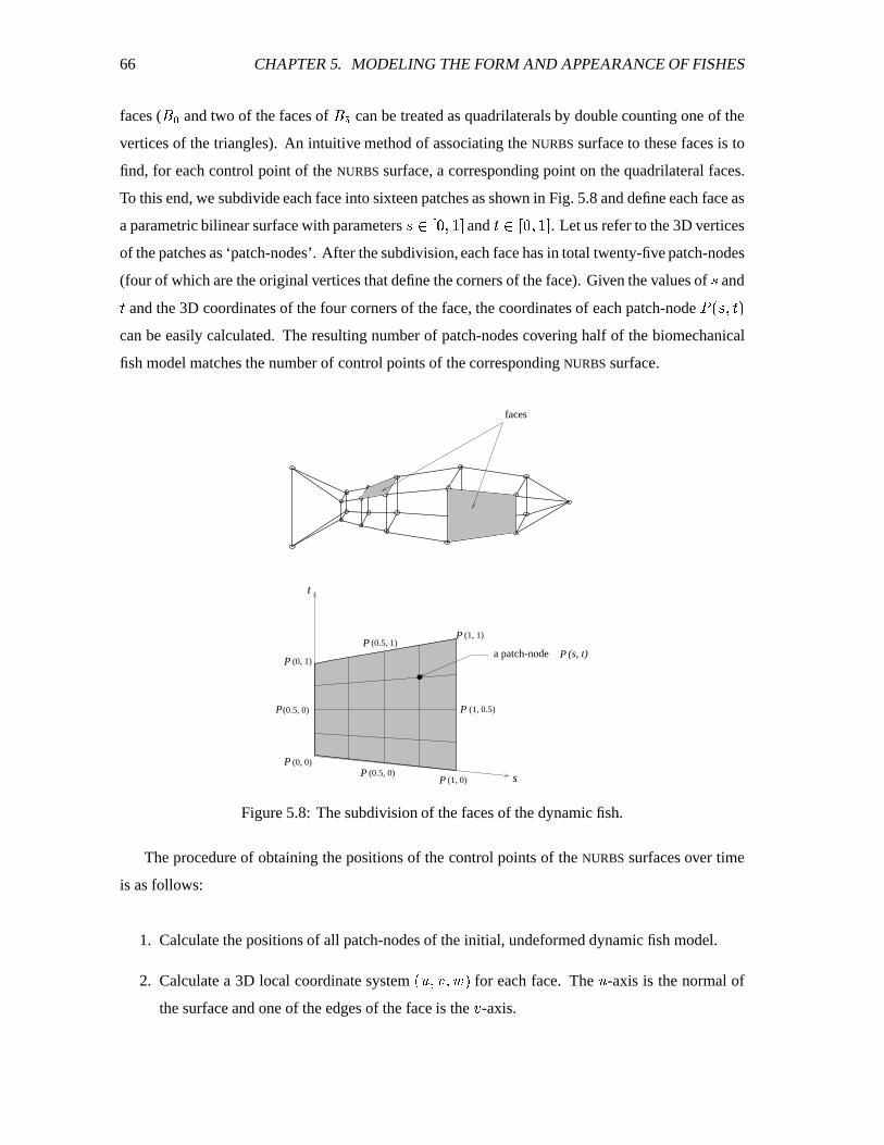
66 CHAPTER 5. MODELING THE FORM AND APPEARANCE OF FISHES
faces ( v and two of the faces of é can be treated as quadrilaterals by double counting one of the
vertices of the triangles). An intuitive method of associating the NURBS surface to these faces is to
find, for each control point of the NURBS surface, a corresponding point on the quadrilateral faces.
To this end, we subdivide each face into sixteen patches as shown in Fig. 5.8 and define each face as
a parametric bilinear surface with parameters ïtdB��\���i�� and d ��\��Qi7� . Let us refer to the 3D vertices
of the patches as ‘patch-nodes’. After the subdivision, each face has in total twenty-five patch-nodes
(four of which are the original vertices that define the corners of the face). Given the values of ï and and the 3D coordinates of the four corners of the face, the coordinates of each patch-nodeü �,ï#����
can be easily calculated. The resulting number of patch-nodes covering half of the biomechanical
fish model matches the number of control points of the corresponding NURBS surface.
(1, 0)
(1, 1)
(0, 1)
(0.5, 0)
(0.5, 0) s
(s, t)
t
faces
(0.5, 1)
(0, 0)
PP
PP
P
P
P
(1, 0.5)P
a patch-node P
Figure 5.8: The subdivision of the faces of the dynamic fish.
The procedure of obtaining the positions of the control points of the NURBS surfaces over time
is as follows:
1. Calculate the positions of all patch-nodes of the initial, undeformed dynamic fish model.
2. Calculate a 3D local coordinate system ������.���P� for each face. The -axis is the normal of
the surface and one of the edges of the face is the � -axis.
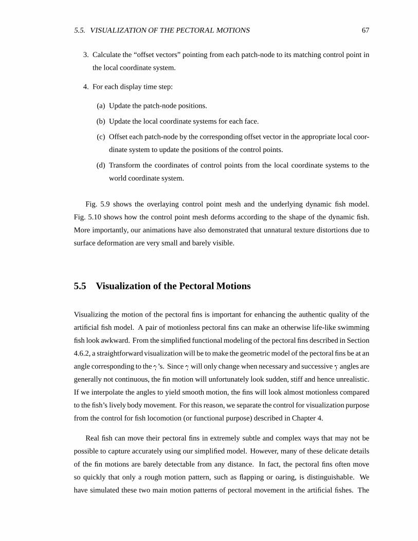
5.5. VISUALIZATION OF THE PECTORAL MOTIONS 67
3. Calculate the “offset vectors” pointing from each patch-node to its matching control point in
the local coordinate system.
4. For each display time step:
(a) Update the patch-node positions.
(b) Update the local coordinate systems for each face.
(c) Offset each patch-node by the corresponding offset vector in the appropriate local coor-
dinate system to update the positions of the control points.
(d) Transform the coordinates of control points from the local coordinate systems to the
world coordinate system.
Fig. 5.9 shows the overlaying control point mesh and the underlying dynamic fish model.
Fig. 5.10 shows how the control point mesh deforms according to the shape of the dynamic fish.
More importantly, our animations have also demonstrated that unnatural texture distortions due to
surface deformation are very small and barely visible.
5.5 Visualization of the Pectoral Motions
Visualizing the motion of the pectoral fins is important for enhancing the authentic quality of the
artificial fish model. A pair of motionless pectoral fins can make an otherwise life-like swimming
fish look awkward. From the simplified functional modeling of the pectoral fins described in Section
4.6.2, a straightforward visualization will be to make the geometric model of the pectoral fins be at an
angle corresponding to the ý ’s. Since ý will only change when necessary and successive ý angles are
generally not continuous, the fin motion will unfortunately look sudden, stiff and hence unrealistic.
If we interpolate the angles to yield smooth motion, the fins will look almost motionless compared
to the fish’s lively body movement. For this reason, we separate the control for visualization purpose
from the control for fish locomotion (or functional purpose) described in Chapter 4.
Real fish can move their pectoral fins in extremely subtle and complex ways that may not be
possible to capture accurately using our simplified model. However, many of these delicate details
of the fin motions are barely detectable from any distance. In fact, the pectoral fins often move
so quickly that only a rough motion pattern, such as flapping or oaring, is distinguishable. We
have simulated these two main motion patterns of pectoral movement in the artificial fishes. The
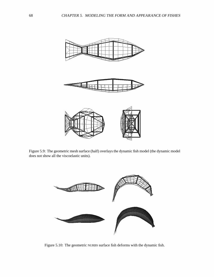
68 CHAPTER 5. MODELING THE FORM AND APPEARANCE OF FISHES
Figure 5.9: The geometric mesh surface (half) overlays the dynamic fish model (the dynamic modeldoes not show all the viscoelastic units).
Figure 5.10: The geometric NURBS surface fish deforms with the dynamic fish.
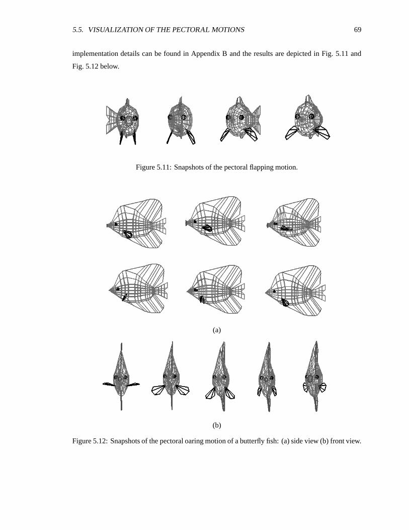
5.5. VISUALIZATION OF THE PECTORAL MOTIONS 69
implementation details can be found in Appendix B and the results are depicted in Fig. 5.11 and
Fig. 5.12 below.
Figure 5.11: Snapshots of the pectoral flapping motion.
(a)
(b)
Figure 5.12: Snapshots of the pectoral oaring motion of a butterfly fish: (a) side view (b) front view.

70 CHAPTER 5. MODELING THE FORM AND APPEARANCE OF FISHES
Chapter 6
Perception Modeling
Perception is at least as crucial a characteristic of animals as is locomotion, for an animal must
perceive its environment in order to survive. Different kinds of animals usually have different
perceptual organs specialized to their particular habitats. Some animals live in the air more than
upon the ground; some prefer bright light while others tend to live more or less in darkness. The
faculties of sense organs can be determined, with relative ease, by studying their structures. However,
it is hard to ascertain how animals actually interpret perceptual information—even for those animals
with rather simple sense organs, perceptual processes are diverse and complex (Smythe, 1975). For
example, birds are known to recognize their mates by the coloration of their feathers, but when such
features are absent they are still able to recognize mates by studying the behavior and the dancing
and posturing which may be associated with courtship.
6.1 Perception Modeling for Animation
Perception modeling for animation is concerned with:
1. Simulating the physical and optical abilities and limitations of the animal’s perception.
2. Interpreting sensory data by simulating the results of perceptual information processing within
the brain of the animal.
When modeling perception for the purposes of animation, our first task is to model the perceptual
capabilities of the animal. Many animals employ eyes as their primary sense organ and perceptual
71
72 CHAPTER 6. PERCEPTION MODELING
information is extracted from retinal images. In an animation system, such “retinal” images corre-
spond to the 2D projection of the 3D virtual world rendered from the point of view of the artificial
animal’s “eyes”. However, many animals do not rely on vision as their primary perceptual mode,
in which case vision models alone may not be able to appropriately capture the animal’s perceptual
abilities.
It is equally important to model the limitations of natural perception. Animal sensory organs
cannot provide unlimited information about their habitats. Most animals cannot detect objects that
are beyond a certain distance away and they usually can detect moving objects much better than
static objects (Tansley, 1965). If these properties are not adequately modeled, unrealistic behaviors
may result.
Moreover, at any moment in time, an animal receives a relatively large amount of sensory
information to which its brain cannot attend all at once. Hence there must be some mechanism
for deciding what particular information to attend to at any particular time. This process is often
referred to as attention. The focus of attention is determined based upon the animal’s behavioral
needs and is a crucial part of perception that directly connects perception to behavior.
Unfortunately, it is not at all well understood how to model animal sensory organs, let alone the
information processing in the brain that mediate an animal’s perception of its world. Fortunately, for
the purposes of animation, an artificial animal in its virtual world can readily glean whatever sensory
information is necessary to support life-like behavior by directly interrogating the world model
and/or exploiting the graphics rendering pipeline. In this way, our perception model synthesizes the
results of perception in as simple, direct and efficient a manner as possible.
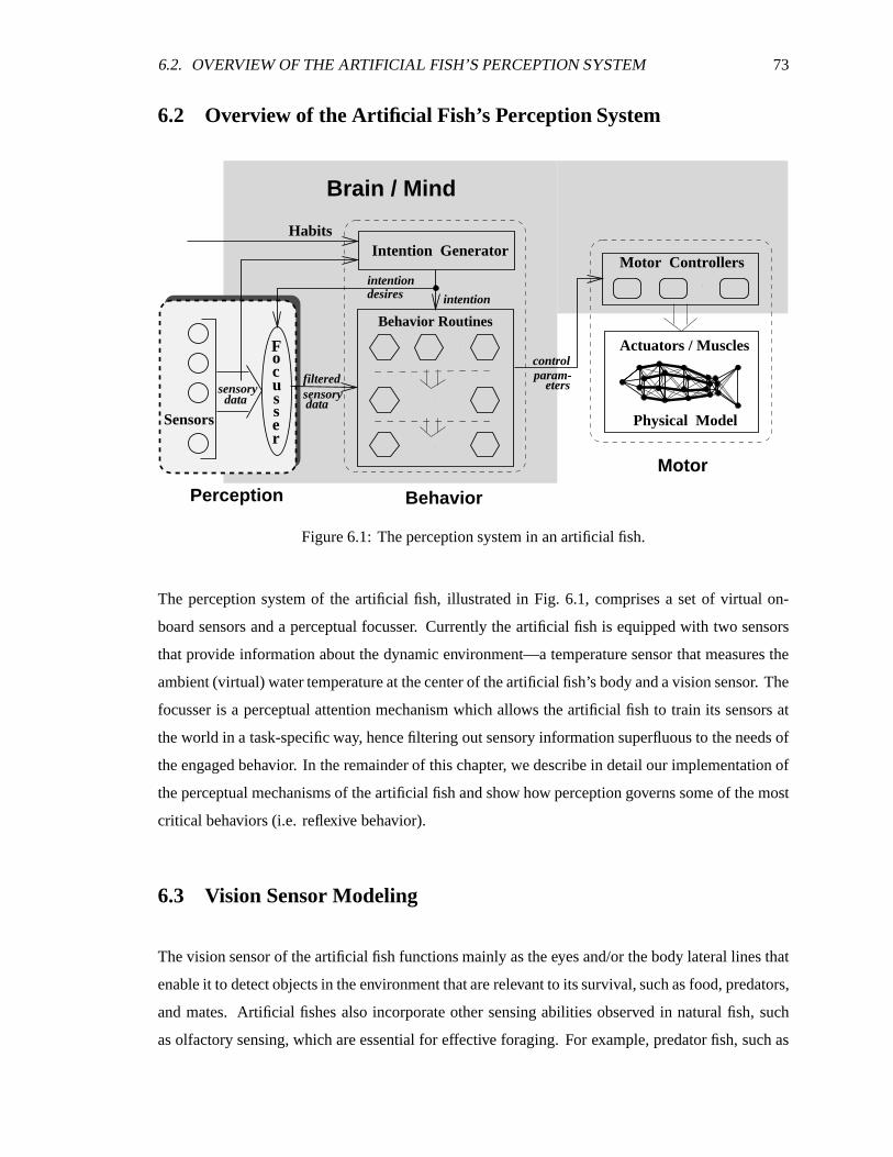
6.2. OVERVIEW OF THE ARTIFICIAL FISH’S PERCEPTION SYSTEM 73
6.2 Overview of the Artificial Fish’s Perception System
Behavior
Motor
Perception
Physical Model
Focu
Actuators / Muscles
Motor Controllers
e
filtered
data
eterssensory
Habits
sensory
Behavior Routines
intention
intentiondesires
data
control
Intention Generator
param-
Brain / Mind
Sensorsss
r
Figure 6.1: The perception system in an artificial fish.
The perception system of the artificial fish, illustrated in Fig. 6.1, comprises a set of virtual on-
board sensors and a perceptual focusser. Currently the artificial fish is equipped with two sensors
that provide information about the dynamic environment—a temperature sensor that measures the
ambient (virtual) water temperature at the center of the artificial fish’s body and a vision sensor. The
focusser is a perceptual attention mechanism which allows the artificial fish to train its sensors at
the world in a task-specific way, hence filtering out sensory information superfluous to the needs of
the engaged behavior. In the remainder of this chapter, we describe in detail our implementation of
the perceptual mechanisms of the artificial fish and show how perception governs some of the most
critical behaviors (i.e. reflexive behavior).
6.3 Vision Sensor Modeling
The vision sensor of the artificial fish functions mainly as the eyes and/or the body lateral lines that
enable it to detect objects in the environment that are relevant to its survival, such as food, predators,
and mates. Artificial fishes also incorporate other sensing abilities observed in natural fish, such
as olfactory sensing, which are essential for effective foraging. For example, predator fish, such as
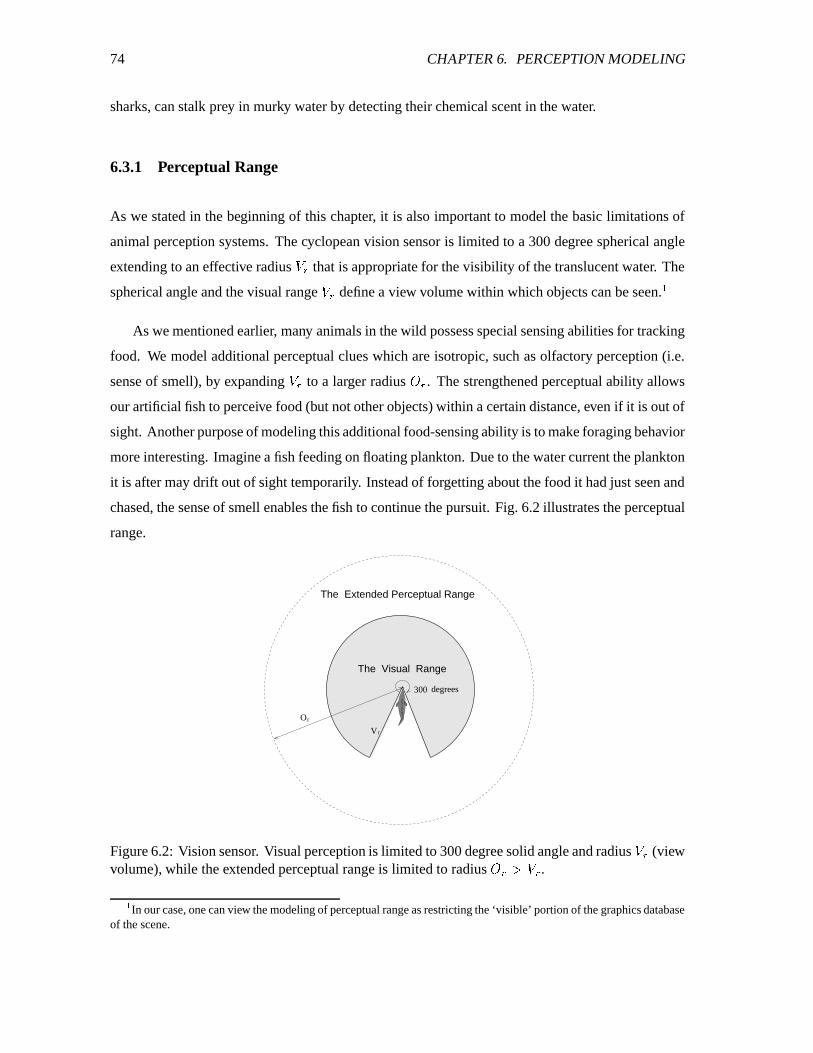
74 CHAPTER 6. PERCEPTION MODELING
sharks, can stalk prey in murky water by detecting their chemical scent in the water.
6.3.1 Perceptual Range
As we stated in the beginning of this chapter, it is also important to model the basic limitations of
animal perception systems. The cyclopean vision sensor is limited to a 300 degree spherical angle
extending to an effective radius ��� that is appropriate for the visibility of the translucent water. The
spherical angle and the visual range ��� define a view volume within which objects can be seen. �As we mentioned earlier, many animals in the wild possess special sensing abilities for tracking
food. We model additional perceptual clues which are isotropic, such as olfactory perception (i.e.
sense of smell), by expanding ��� to a larger radius ��� . The strengthened perceptual ability allows
our artificial fish to perceive food (but not other objects) within a certain distance, even if it is out of
sight. Another purpose of modeling this additional food-sensing ability is to make foraging behavior
more interesting. Imagine a fish feeding on floating plankton. Due to the water current the plankton
it is after may drift out of sight temporarily. Instead of forgetting about the food it had just seen and
chased, the sense of smell enables the fish to continue the pursuit. Fig. 6.2 illustrates the perceptual
range.
The Extended Perceptual Range
300 degrees
V
O
r
r
The Visual Range
Figure 6.2: Vision sensor. Visual perception is limited to 300 degree solid angle and radius ��� (viewvolume), while the extended perceptual range is limited to radius ��������� .�In our case, one can view the modeling of perceptual range as restricting the ‘visible’ portion of the graphics database
of the scene.
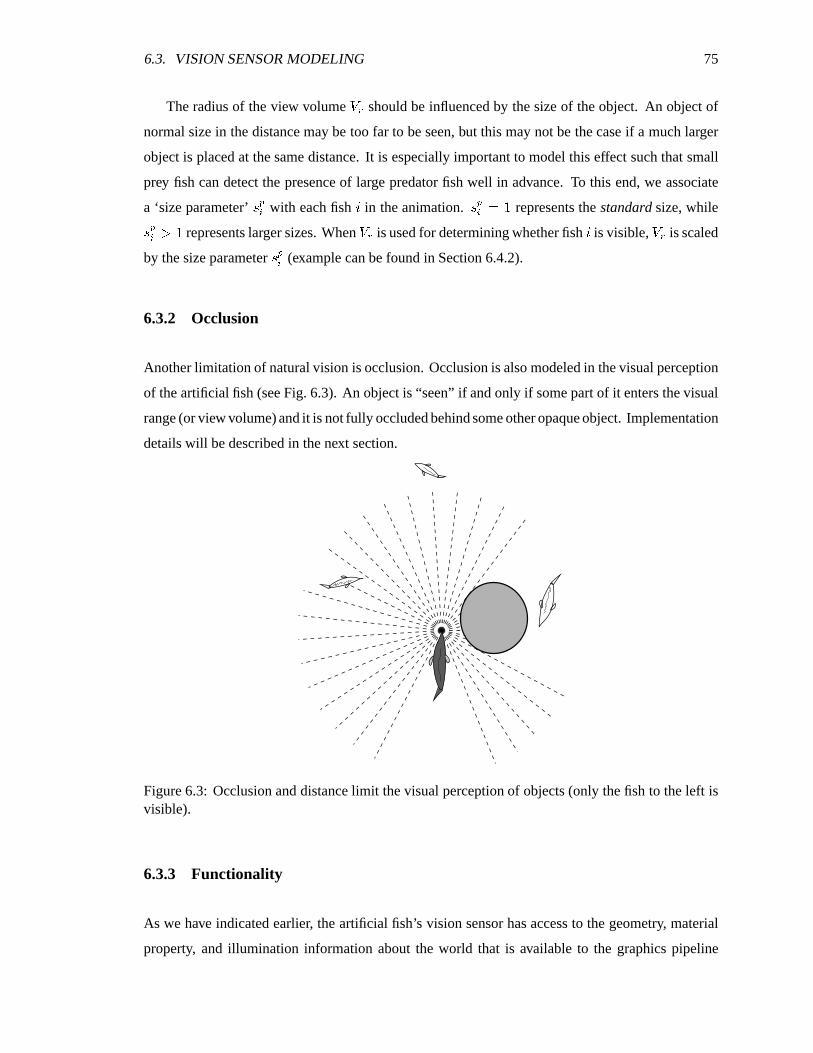
6.3. VISION SENSOR MODELING 75
The radius of the view volume � � should be influenced by the size of the object. An object of
normal size in the distance may be too far to be seen, but this may not be the case if a much larger
object is placed at the same distance. It is especially important to model this effect such that small
prey fish can detect the presence of large predator fish well in advance. To this end, we associate
a ‘size parameter’ ��� � with each fish � in the animation. ��� ���! represents the standard size, while
� � �"�# represents larger sizes. When � � is used for determining whether fish � is visible, � � is scaled
by the size parameter ��� � (example can be found in Section 6.4.2).
6.3.2 Occlusion
Another limitation of natural vision is occlusion. Occlusion is also modeled in the visual perception
of the artificial fish (see Fig. 6.3). An object is “seen” if and only if some part of it enters the visual
range (or view volume) and it is not fully occluded behind some other opaque object. Implementation
details will be described in the next section.
Figure 6.3: Occlusion and distance limit the visual perception of objects (only the fish to the left isvisible).
6.3.3 Functionality
As we have indicated earlier, the artificial fish’s vision sensor has access to the geometry, material
property, and illumination information about the world that is available to the graphics pipeline
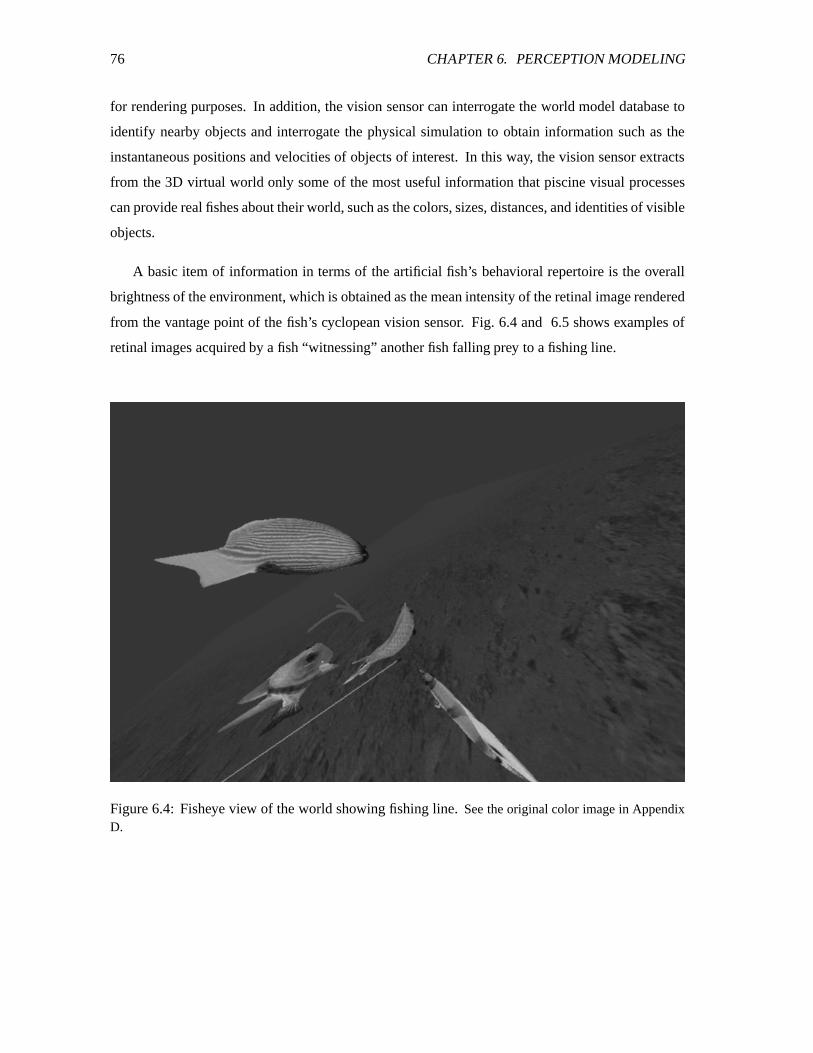
76 CHAPTER 6. PERCEPTION MODELING
for rendering purposes. In addition, the vision sensor can interrogate the world model database to
identify nearby objects and interrogate the physical simulation to obtain information such as the
instantaneous positions and velocities of objects of interest. In this way, the vision sensor extracts
from the 3D virtual world only some of the most useful information that piscine visual processes
can provide real fishes about their world, such as the colors, sizes, distances, and identities of visible
objects.
A basic item of information in terms of the artificial fish’s behavioral repertoire is the overall
brightness of the environment, which is obtained as the mean intensity of the retinal image rendered
from the vantage point of the fish’s cyclopean vision sensor. Fig. 6.4 and 6.5 shows examples of
retinal images acquired by a fish “witnessing” another fish falling prey to a fishing line.
Figure 6.4: Fisheye view of the world showing fishing line. See the original color image in AppendixD.
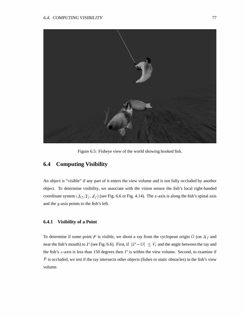
6.4. COMPUTING VISIBILITY 77
Figure 6.5: Fisheye view of the world showing hooked fish.
6.4 Computing Visibility
An object is “visible” if any part of it enters the view volume and is not fully occluded by another
object. To determine visibility, we associate with the vision sensor the fish’s local right-handed
coordinate system $&%('*)�+�'�)-,.'0/ (see Fig. 6.6 or Fig. 4.14). The 1 -axis is along the fish’s spinal axis
and the 2 -axis points to the fish’s left.
6.4.1 Visibility of a Point
To determine if some point 3 is visible, we shoot a ray from the cyclopean origin � (on %4' and
near the fish’s mouth) to 3 (see Fig. 6.6). First, if 5657398:�;5<5>=?��� and the angle between the ray and
the fish’s 1 -axis is less than 150 degrees then 3 is within the view volume. Second, to examine if
3 is occluded, we test if the ray intersects other objects (fishes or static obstacles) in the fish’s view
volume.
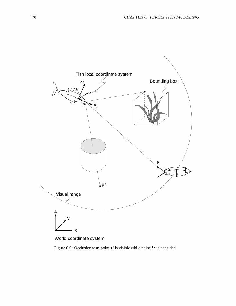
78 CHAPTER 6. PERCEPTION MODELING
x
yf
zf
of
Z
p’
p
Fish local coordinate system
Visual range
Bounding box
World coordinate system
X
Y
Figure 6.6: Occlusion test: point 3 is visible while point 3�@ is occluded.
6.4. COMPUTING VISIBILITY 79
Occlusion Test
Fishes are generally vigorous animals that move around constantly. If at some instant the sight
of one fish is blocked by another fish passing by, the occlusion will most likely be cleared soon
after—since both fish are in motion. The temporary blocking of sight should not result in abrupt
changes in a fish’s behavior. Therefore, occlusion tests against another fish tend to be unessential.
To increase computational efficiency, the artificial fish performs occlusion tests only against large
static environmental objects. In the current implementation, this includes cylindrical objects. Note
that, for obstacles with more complex geometric shapes, cylinders can serve as their bounding boxes.
The algorithm for testing the intersection of a ray with a cylinder is simple, especially since the
axis of each cylinder is parallel to the A -axis of the world coordinate system (see Fig. 6.6). Let the
coordinates of � and 3 in the world coordinate system be denoted by $�1�B-)C2DB-)�AEBF/ and $G1 � )C2 � )CA � / ,respectively. Then line �H3 can be represented by the parametric equation
1:�I1�BKJMLE®(1N)O2P�I2DBQJML,®(2�)OAP�RASBQJ9LE®(AT) (6.1)
where ®41U�I1 � 8U1�B , ®(24�I2 � 8U2DB , ®(A��IA � 8UAEB and LWVMXZYT)E -[ . Let \ denote the radius and ] the
height of the cylinder ^ under consideration. Its projection onto the %_+ -plane is a circle ` which
can be represented by the parametric equation
$�148baT/�c.J�$G2"8bdS/�ce�f\gc (6.2)
where $�a�)CdD)CYh/ denotes the center of ` . The occlusion-test algorithm we develop can be outlined as
follows (all calculations are performed in the world coordinate system):
1. Check if line �H3 intersects with circle ` :
Substitute the 1 and 2 in Eq. (6.2) with those in Eq. (6.1) and solve for L . If the solutions L �and L c ( L � =RL c ) have real values and at least one of them is in XZYT)E -[ , then do step 2; Otherwise,stop ( 3 is not occluded by cylinder ^ ).
2. Further check if line ��3 intersects with cylinder ^ :
Substitute the L in Eq. (6.1) with L � and L c to get the points of intersection. In fact, one only
needs to calculate A � �fA B JML � ®(A , �K�i 0)�j . If Y(k?A � =?] for �K�i or �K�Ij , then point 3 is
occluded. Otherwise, 3 is visible.
This algorithm is essentially an ‘extent testing’ algorithm commonly used in determining visibility
80 CHAPTER 6. PERCEPTION MODELING
of objects in a scene (Foley et al., 1990).
6.4.2 Visibility of Another Fish
To determine the visibility of another fish, we take advantage of the mass-spring-damper structure
of the fish model. To first determine if fish l is within fish � ’s view volume, we simply test if the
center of l ’s body mon (we use the origin of the fish local coordinate system $&%('*)�+�'�)-,.'D/ as the
center point) falls within the view volume of � (Note that, the view volume of fish � is ���n ��� instead
of � � ). If it is, we proceed as follows: Fish l is visible to fish � if and only if any one of the mass
points of l is visible to � (i.e. not occluded by any other objects). In Fig. 6.6, the fish represented by
the mass-spring-damper model is visible. It should be pointed out that, although in the worst case
this visibility check can be expensive (each fish has 23 nodes), on average it is much better since
the algorithm will reach a conclusion as soon as it finds a single visible node. In the case of a more
complicated virtual environment, we can use bounding box techniques to speed up the occlusion
test.
6.4.3 Visibility of a Cylinder
Since a full visibility check for a cylinder would be computationally expensive, we perform the
following simple test: Let 3 be the point on the axis of cylinder ^ that is closest in height to the
cyclopean origin � . Then we say that ^ is visible if 5<573p8b�q565D8b\;kf��� , where \ is the radius of
^ . Since the cylinders in a typical virtual marine world in our animation are fairly scattered, the
occlusion test is neglected.
6.4.4 Visibility of Seaweeds
In our animated marine world, we model clustered seaweeds (multiple leaves originated from the
same root) that are often observed in nature. To perform efficient visibility check of seaweeds, we
use a rectangular bounding box for each seaweed cluster (see Fig. 6.6). The visibility of a seaweed
cluster is determined by the visibility of the 8 corners of the corresponding bounding box. If any of
the corner points is visible, the seaweed cluster is visible.
6.4. COMPUTING VISIBILITY 81
6.4.5 Discussion
To summarize, in order to model an artificial fish’s perceptual capability, at each animation time
step, a visibility check with all environmental objects is performed. As we described above, the
visibility check consists of two steps: First, the view volume test checks if an object is in the fish’s
view volume and, if it is, the occlusion test checks whether it is occluded.
Since the occlusion test algorithm is only performed against, hopefully, a small number of
objects that fall within the fish’s view volume, the corresponding computational cost does not
increase linearly with the total number of objects in the scene. However, this is not true for the
computation in the view volume test: If a naive algorithm is used, the computational cost involved
(for each fish) is �P$�rs/ where r is the number of objects in the scene. The total cost for all the fish
performing the view volume test will increase quadratically with the number of fish in the animation.
Therefore, when the number of fish is large, for example, when animating a school of fish, a more
efficient algorithm for the view volume test is desirable. To this end, we have implemented an
algorithm that exploits the space-time coherence of objects. We associate, with each fish, a list of
potentially-visible objects. One can view the potentially-visible objects as those that fall within a
pseudo view volume that has a larger radius than that of the fish’s view volume. This list is generated
at the beginning of the animation and is only updated intermittently. At each animation time step,
assuming constraints on the maximum fish velocity, instead of performing the view volume test on
all the other objects, a fish need only check if any of the objects in the list of potentially-visible
objects enters the view volume.
It is important to appreciate, however, that the value of our perception model does not lie
in the particular method we choose to implement it. (Indeed, to achieve high simulation speed
for animation, we have chosen a very simple approach which may not be readily extensible to a
more complex virtual environment.) Rather our main purpose is to demonstrate the importance
of simulating perceptual capability to the modeling of realistic behavior and, in this respect, our
approach is adequate for the task at hand.
One avenue for future research would be to implement a more sophisticated geometric method
that can scale well to more complicated virtual environments. For instance, we could tessellate the
entire 3D environment into, say, t cells and establish a look-up table with t entries. Each entry of
the table registers the indices of objects that reside in the corresponding cell. This table is computed
at the beginning of the animation and is updated for each fish at each time step. Because of the
space-time coherence, the update need not be computed with respect to all the cells. Rather only
82 CHAPTER 6. PERCEPTION MODELING
the adjacent cells are checked to see in which new cell the fish is currently situated. Once the table
is updated, the objects that fall within a fish’s view volume can be easily determined by accessing
the table entries of those cells that are nearby. This algorithm is especially suitable if there is a large
number of objects besides fish, such as static obstacles, seaweeds, etc.
Moreover, for the occlusion test, more sophisticated bounding volume algorithms, such as the
Kay-Kajiya algorithm (Foley et al., 1990), can be employed when the shape of the obstacles is more
complicated.
6.5 The Focusser
The task of a focus of attention mechanism is to extract the appropriate aspects of the world for the
particular tasks with which the animal/agent is concerned. Robotics and computer vision researchers
have proposed a number of computational models of attention mechanisms for various applications
(Tsotsos et al., 1995). Modeling focus of attention in artificial animals is important for modeling
their behavior as well as for gaining high computational efficiency in sensory processing.
6.5.1 Focus of Attention in Animals
Animals are believed to focus their attention in two ways. The first, which is most common in lower
animals, is the use of specialized sensing organs. Many of these animals have severely limited, but
highly specialized vision which allow them to see just what they need to see in order to function
successfully in their environments (Tansley, 1965). For example, anteater’s eyes are placed very
low in their heads and they have only monocular vision but with extremely high acuity. Birds, on
the other hand, have excellent binocular vision that is good for judging distances. The second way
can be thought of as cognitive, where the animals only perceive what they attend to; i.e., they pay
attention only to what is important in their particular situation at hand.
Under certain circumstances nesting herring-gulls behave as though their eggs were
invisible to them. If, in the gull’s absence, the eggs are removed and put just outside
the nest the parent bird will retrieve them, but if the distance is made a little greater the
bird will sit happily on the empty nest with the eggs in full sight. That the eggs can be
seen perfectly well is indicated by removing them still further away, the gull will then
eat them as it does its neighbour’s eggs if it should find them unguarded. Herring-gull
6.5. THE FOCUSSER 83
chicks show camouflage colouring very similar to that of the eggs but the parent bird
never has any difficulty in seeing and recognizing its own chicks. There is nothing
wrong with the herring-gull’s eyes. The explanation of the different reactions to eggs
and chicks appears to be that, under normal circumstances, the eggs do not leave the
nest and it is, therefore, sufficient if the parent knows the position of the nest, while the
active chicks often wander away and have to be got back (Tansley, 1965).
The best example of a natural attention mechanism that employs both mechanical and cognitive
means may lie in the vision of humans and animals. The retinal image from an eye has in its center
a high-acuity region known as the fovea, beyond which the image resolution drops in the visual
periphery. Humans and animals, motivated by their behavioral needs, are able to focus their sight
(by moving their eyes or turning their heads) onto the object of interest such that an accurate image
of that object is obtained in their foveas while its immediate surroundings fall into the low-resolution
peripheral region.
6.5.2 Design of the Focusser
The design of the focusser is inspired by the functioning of the eyes. It synthesizes the foveal vision
by suppressing sensory information unrelated to object(s) of interest. It also synthesizes peripheral
vision by generating qualitative motor preferences from related environmental conditions. As we
shall see, the motor preferences are important to the artificial animal’s behavior.
Obtaining the Focus
As we shall describe in the next chapter, an intention generator in the artificial fish’s brain generates
an intention of what to do next at each animation time step. The functioning of the focusser is
controlled by the time-varying intention of the fish. When the intention is to avoid collision, the
focusser is activated to locate the position of the most dangerous obstacle, usually the closest, among
all the dangerous obstacles perceived (we will explain the determination of dangerous obstacles in
the next section). The focusser passes only the position of the most dangerous obstacle to the
behavior system. Likewise, when the intention of a male fish is to mate, the focusser targets the most
desirable female fish; when the intention is to escape from predators, only the detailed information
about the most threatening predator gets passed through the focusser.
84 CHAPTER 6. PERCEPTION MODELING
Motor Preferences
The above simple attention mechanism passes only the directly required information for fulfilling
the animal’s current intention. While this is highly efficient, it neglects some desirable sensory
information necessary for better accomplishing the task at hand, or for taking compromised actions
towards satisfying more than one intention. An important characteristic of animal behavior is to
be able to select compromised actions from the consideration of multiple aspects of the animal’s
behavior and its environment (Tyrrell, 1993b). In order to capture this feature in an artificial animal’s
behavior model, sensory information in addition to that provided about the object of focus is required.
Example 1:
Take for example the case where a fish intends to avoid collisions with surrounding obstacles, among
which one presents the highest danger of collision (usually the closest). In most situations, the fish
would have several choices of actions that it can take to maneuver around that obstacle: it can turn
left, turn right, retreat, etc. Further assume that there is another nearby obstacle (either mobile or
static) which is to the left of the fish and a food source to the right. With the focusser described
above, sensory information about this other obstacle and the food source will be filtered out and
hence cannot contribute to the decision about the choice of action. However, by considering the
presence of this additional sensory information, the obvious choice of action would be to take a right
turn. If the fish retreats, it cannot take advantage of eating food. If it takes a left turn the obstacle
to the left would immediately become the next “most dangerous” obstacle and hence, in the worst
case, the fish would dither back and forth.
Example 2:
Another example is concerned with attempting to satisfy multiple desires. Imagine that a hungry
fish is chasing floating food particles. Assume the simple case of two food particles, one located
straight ahead and closer to the fish, and the other a little further and to the left of the fish. Under
normal conditions, the fish will focus its attention on the food that requires the least amount of
effort to get—the particle in front of it. However, suppose the fish has also a desire to mate and it
sees a potential mate to its left, then a better choice (a compromised choice) of action may be to
turn left—such that it can eat food while approaching the potential mate. This also depends on the
relative strength of the desire to mate compared to the intention to eat.
It is clear that additional information about the environment is necessary for selecting preferred
strategies of action. But how accurate and complete should additional information about the
environmental objects be?
6.5. THE FOCUSSER 85
At one end of the spectrum we could use a complete, accurate description (i.e., 3D positions,
velocities, etc., of all relevant objects), it is possible to decide on an ‘optimal’ action at a given
moment, such as “turn right 23.65 degrees”. However, this will involve high computational cost
and hence offset the benefits of focus of attention. In addition, the artificial fish’s motor system,
like those of many real animals, cannot produce motions more accurate than, say, turn roughly 45
degrees. Therefore excessively accurate motor commands tend to be futile. At the other end of the
spectrum we could have no additional information whatsoever, but as we have already stated, this is
undesirable. So the question remains: What level of granularity should our system have in between
the two extremes? Inspired by the fact that the peripheral vision of the human eye, although of
poor accuracy, serves the necessary purpose. We chose to represent the additional information as
qualitative recommendations of actions, henceforth referred to as motor preferences.
Instead of passing all the sensory information about the surroundings, the focusser computes
and collects a set of motor preferences. The set of motor preferences corresponds to the set of motor
skills of the artificial fish, namely,�����������
,� ������������
,� �����������������
,� �������������������
,����������������
,����������������� �.
First let us distinguish the concept of ‘intention’ from that of ‘desire’. Desires are potential
candidates of the intention. At any given moment, an agent can have multiple desires, but there
will be only one intention which corresponds to the strongest desire. Now if a sensory stimulus
relevant to a desire/intention occurs, a value is assigned to the appropriate motor preference. A
positive value represents a positive recommendation for the action, and a negative value represents
negative recommendation for the action. For instance, if an obstacle is close and is in front of the
fish, a negative value will be assigned to���!���������������
. The magnitude of the value is given by a
factor "$#&%('�)+*-, representing the strength of that desire. The final value of a motor preference will
be a normalized sum of all the assigned values from different desires. The summation is performed
first on all the positive recommendations and then on all negative recommendations. These two
summations are individually normalized and then added together. For example, suppose a fish
perceives three potential mates to its left and the desire to mate has strength "�. (we will describe
how the " ’s are calculated in Section 7.6 in Chapter 7). Now further suppose that the fish also
detects a predator to its left and the desire to flee has strength "�/ . Then the motor preference�����������102�!3 " .54 3��76 " / 0 " . 6 " / . Therefore, in the first example described above, there are
two motor preferences:�����������8096 "�: ( : represents the desire to avoid collision) and
�������;�����0 "�< ( < represents the desire to eat).
86 CHAPTER 6. PERCEPTION MODELING
6.5.3 Summary
To summarize, the focusser delivers to the appropriate behavior component the accurate sensory
information about the object of interest as well as the motor preferences reflecting the current
environmental conditions. This design not only provides highly focussed attention for efficiency,
but also allows influence from environmental conditions to achieve compromised actions.
As is indicated by the examples in the previous section, motor preferences are used in two
ways. In the first way they are used to influence the choice of a proper action. This is done by
influencing both the selection of a proper motor skill (e.g., example 1 above) and the calculation of
the corresponding control parameters. In the case where all possible actions are accompanied by
equal-strength negative motor preferences, an action gets chosen at random and the corresponding
control parameters (angle or speed) are modified to accommodate the preference. For example,
suppose the =?>+@A�B C�B�D�=EFC ��� is chosen and the calculated angle of turn is G , since�������;�����H0I6 " ,
the final, compromised angle of turn will be JLKNMH%O*�P('�) � *PRQ 6 " � ,OG . Similar modification of motor
control parameters is also performed in the case where the chosen action is accompanied by a
negative preference. Positive preferences do not have any effect on the control parameters.
In the second way, the motor preferences are used to help the focusser locate the object of
interest. This process demonstrates a certain level of compromise among different desires. Typical
cases include targeting the most desirable food source and mating partner. In each case, there is an
evaluation criterion according to which a real valued ‘desirability’ SLTU#V%R'�)W*-, is calculated for each
potential target X (i.e. food source or mate). Assuming *ZY[X1Y]\ where \ is the number of potential
targets, then the procedure for choosing the most desirable target can be specified in pseudo code
(D[i] represents S T ):
6.6. FROM PERCEPTION TO BEHAVIOR 87
^�_ =a`W>]bdcfegEHhi _ =�Bj` �lk >Wm?hHn$o�o �lk c-m[A?p i BAFqsr p�=�@�q i But p�r;DFqjv> ^ `�E b�bFcxw�w �lk c-m�y�y �lk!z mFhB�p{=�@�q{B|e�b}c~nq�r i q]�� e�b���>�E k��8� E�m8nVo�o � > i p i �Hp�r�rI>�E�B q�@ q�=lv ��� >��p�r�r �8��� b��1v^�_ =a`��Ib�cHe � h]���p;r �+D r p{B�q � q�r�� _ i k ��m8n�o�o � q;r� _ i k ��m�> i BAFq[= q�r�p�B?>+t�q � _ i >WB?> _ E _^ `��Fh�B _u^ > i A�vo�o � q�r�� _ i ��pWE�AFp�t�q�BA�= q�q�t p�r�D?q i e�r q ^ B � =?>+@A�B ��^ = _ E�Blv� e�b��8v z n o�o�> i p i �fp�r�ru��q�>+@A�B ^ p���B _ =lv�lk ��mI��b �?��� ` � q�r� _ i k ��mFhfn�o�o � ` ^ = _ E�BFh�b � ` � �{��������� hUv�^�_ =a`��Ib�cHe � h�lk >Wm�e�b&�fp���� ��k ��m � nB�p{=�@�q{B|e�bI>fn�The desirability calculation for a food source is, for simplicity, solely based on its distance to
the fish. Let �T be the distance of food X to the fish, then SLT 0 *�P(' 6 �T 4���� where ��� is the
fish’s perceptual range described earlier. The desirability of a mating partner will be described in
Section 7.9.3.
6.6 From Perception to Behavior
The perception system supports a range of fish behaviors, such as foraging and escaping from
predation. This section describes how perception supports behavior through the example of collision
avoidance — the most basic perception-driven behavior in the artificial fish’s behavior repertoire.
6.6.1 An Example: Collision Detection
Collision avoidance is essential for the day to day life of animals. Their survival needs compel them
to move around constantly. To be able to do so safely, an animal’s perception must first provide an
account for collision detection.
Analogous to all animals and humans, the avoidance of collisions with obstacles is a primitive
behavior that an artificial fish performs. Once a static obstacle or another fish comes into view,
the artificial fish must determine if there is potential for a collision and, if so, act to avoid the
collision. As will be shown in Chapter 7, the collision detection algorithms described below support
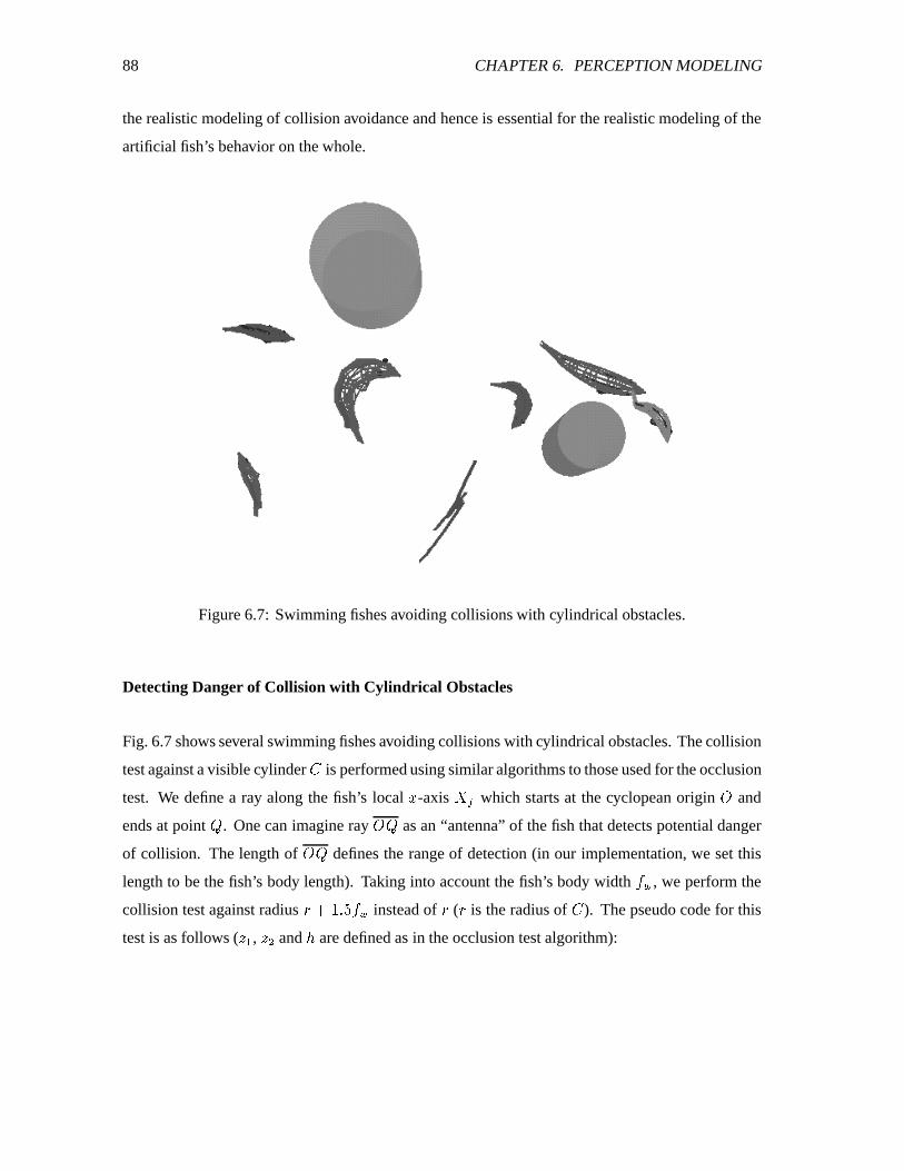
88 CHAPTER 6. PERCEPTION MODELING
the realistic modeling of collision avoidance and hence is essential for the realistic modeling of the
artificial fish’s behavior on the whole.
Figure 6.7: Swimming fishes avoiding collisions with cylindrical obstacles.
Detecting Danger of Collision with Cylindrical Obstacles
Fig. 6.7 shows several swimming fishes avoiding collisions with cylindrical obstacles. The collision
test against a visible cylinder is performed using similar algorithms to those used for the occlusion
test. We define a ray along the fish’s local ¡ -axis ¢ / which starts at the cyclopean origin � and
ends at point £ . One can imagine ray � £ as an “antenna” of the fish that detects potential danger
of collision. The length of � £ defines the range of detection (in our implementation, we set this
length to be the fish’s body length). Taking into account the fish’s body width ¤W¥ , we perform the
collision test against radius ¦5§u*�PRQ�¤ ¥ instead of ¦ ( ¦ is the radius of ). The pseudo code for this
test is as follows ( ¨�© , ¨+ª and « are defined as in the occlusion test algorithm):
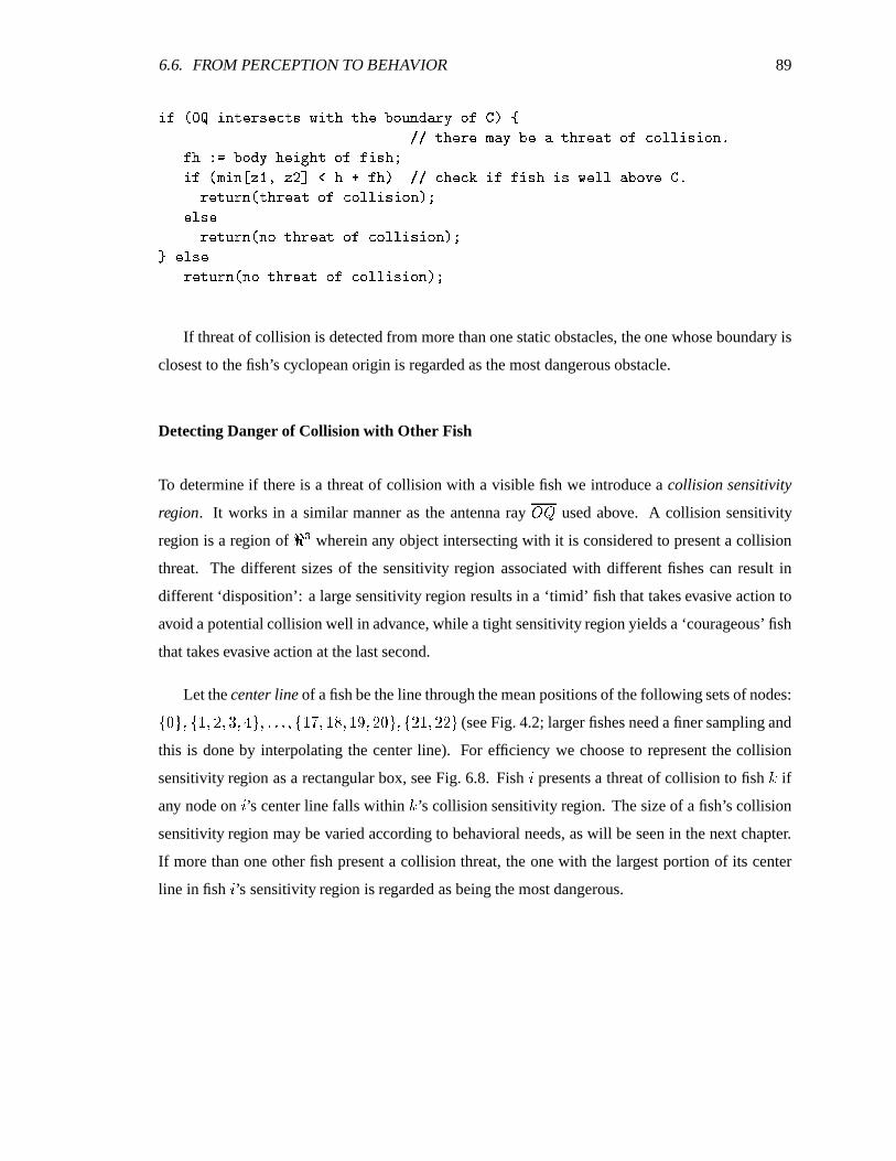
6.6. FROM PERCEPTION TO BEHAVIOR 89
> ^ ` ��¬ >-E�B�q{= i q���B i �?>+BA�B�A?q� _ D�E ® p{= ��_�^I� h��o�o�B�A?q�= q&�fp � ?q�p�BA�=�q�p�B _�^ � _ r�r�> i > _ E5v^ A�e�b[ _ ® � AFq�>+@A�B _^�^ > i Aln> ^ `���>�E k�¯ c ��¯�z m±°�A�� ^ AHh o�ou�+A?q��{�d> ^u^ > i A9> i ��q;r�r²p+ _ t q � v= q�B�D�=E³`�B�A�=�q�p�B _^ � _ r�r > i > _ E~hfnq;r i q= q�B�D�=E³`´E _ BA�=�q�p{B _^ � _ r�r > i > _ E~hfn� q�r i q= q�BD�=E³`´E _ BA�=�q�p�B _�^ � _ r�r�> i > _ EHhfnIf threat of collision is detected from more than one static obstacles, the one whose boundary is
closest to the fish’s cyclopean origin is regarded as the most dangerous obstacle.
Detecting Danger of Collision with Other Fish
To determine if there is a threat of collision with a visible fish we introduce a collision sensitivity
region. It works in a similar manner as the antenna ray � £ used above. A collision sensitivity
region is a region of µl¶ wherein any object intersecting with it is considered to present a collision
threat. The different sizes of the sensitivity region associated with different fishes can result in
different ‘disposition’: a large sensitivity region results in a ‘timid’ fish that takes evasive action to
avoid a potential collision well in advance, while a tight sensitivity region yields a ‘courageous’ fish
that takes evasive action at the last second.
Let the center line of a fish be the line through the mean positions of the following sets of nodes:· '�¸�) · *�)º¹�) 3 )�»�¸�)WP-P-P!) · *�¼�)W*+½�)-*+¾ )¿¹�'�¸�) · ¹�*�)¿¹¹�¸ (see Fig. 4.2; larger fishes need a finer sampling and
this is done by interpolating the center line). For efficiency we choose to represent the collision
sensitivity region as a rectangular box, see Fig. 6.8. Fish X presents a threat of collision to fish À if
any node on X ’s center line falls within À ’s collision sensitivity region. The size of a fish’s collision
sensitivity region may be varied according to behavioral needs, as will be seen in the next chapter.
If more than one other fish present a collision threat, the one with the largest portion of its center
line in fish X ’s sensitivity region is regarded as being the most dangerous.
90 CHAPTER 6. PERCEPTION MODELING
f
Sensitivity Region
X
Z f
f
Y
Figure 6.8: The fish’s collision sensitivity region.
6.7 Synthetic Vision Models
As we have mentioned earlier, when the virtual environment becomes highly complex, for example,
when the shapes of the obstacles or other objects are highly irregular, more sophisticated geometric
methods for perception modeling can be employed. An alternative approach to geometric methods
is one that involves building synthetic vision models of animals.
In the context of artificial life, we may also be interested in developing models of animal vision
that are biologically more faithful. For instance, we may be interested in modeling the process of
extracting useful perceptual information from the retinal images of an animal’s vision system and
studying how this process affects an animal’s behavior.
Synthetic vision models can be built based on the animated retinal images rendered from an
artificial animal’s “point of view”. One obvious advantage of this approach is that the retinal
images readily respect the occlusion relationships between objects in the animal’s view. In addition,
these retinal images are perspective projections of the 3D virtual world and hence are biologically
plausible models of animal vision. Some aspects of animal perception, such as the recognition
of object textures or environmental illumination, cannot be captured by geometric methods but
are unique properties that have to be extracted from images. The synthetic vision approach for
animation was first explored by Renault, Magnenat-Thalmann, and Thalmann (1990) in guiding
synthetic actors’ navigation through a dynamic world.
A simple procedure of synthetic vision is to render each object in the scene with a unique shaded
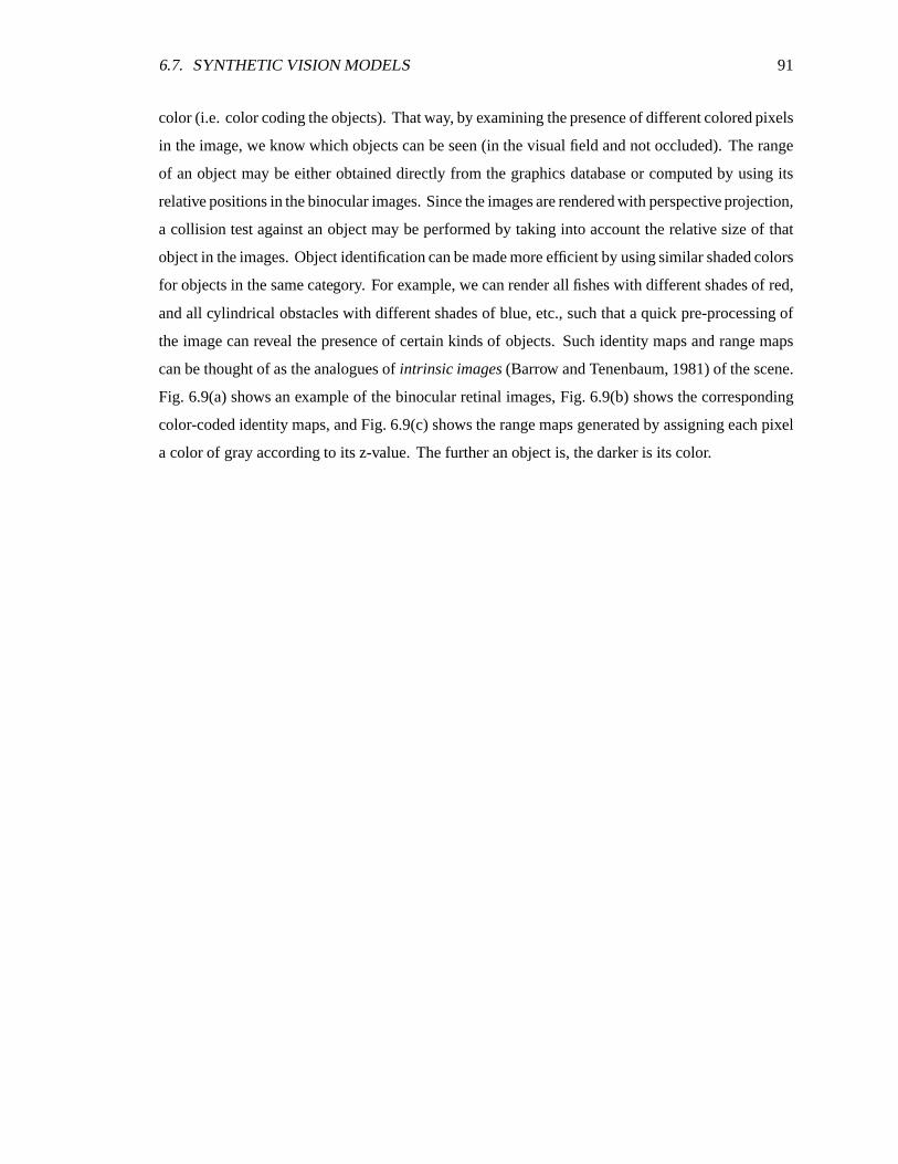
6.7. SYNTHETIC VISION MODELS 91
color (i.e. color coding the objects). That way, by examining the presence of different colored pixels
in the image, we know which objects can be seen (in the visual field and not occluded). The range
of an object may be either obtained directly from the graphics database or computed by using its
relative positions in the binocular images. Since the images are rendered with perspective projection,
a collision test against an object may be performed by taking into account the relative size of that
object in the images. Object identification can be made more efficient by using similar shaded colors
for objects in the same category. For example, we can render all fishes with different shades of red,
and all cylindrical obstacles with different shades of blue, etc., such that a quick pre-processing of
the image can reveal the presence of certain kinds of objects. Such identity maps and range maps
can be thought of as the analogues of intrinsic images (Barrow and Tenenbaum, 1981) of the scene.
Fig. 6.9(a) shows an example of the binocular retinal images, Fig. 6.9(b) shows the corresponding
color-coded identity maps, and Fig. 6.9(c) shows the range maps generated by assigning each pixel
a color of gray according to its z-value. The further an object is, the darker is its color.
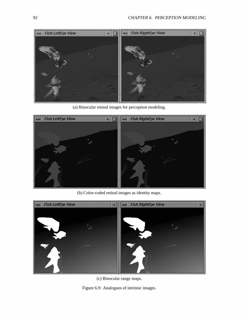
92 CHAPTER 6. PERCEPTION MODELING
(a) Binocular retinal images for perception modeling.
(b) Color-coded retinal images as identity maps.
(c) Binocular range maps.
Figure 6.9: Analogues of intrinsic images.
Chapter 7
The Behavior System
Action selection in the artificial fish is controlled by its behavior system. The behavior system
consists of the habits and mental state of the fish, an intention generator and a set of behavior
routines (Fig. 7.1). The behavior system runs continuously within the fish’s simulation loop. At
each time step the intention generator issues an intention based on the fish’s habits, mental state, and
incoming sensory information. It then chooses and executes a behavior routine which in turn selects
and runs the appropriate motor controllers. It is important to note that the behavior routines are
incremental by design. Their job is to get the artificial fish one step closer to fulfilling its intention
during the current time step. Moreover, at any given moment in time, there is only one intention
or one active behavior in the artificial fish’s behavior system. This hypothesis is commonly made
by ethologists when analyzing the behavior of fishes, birds and four-legged animals of or below
intermediate complexity (e.g. dogs, cats) (Tinbergen, 1951; Manning, 1979).
In this chapter, we first list a set of design criteria for effective action selection mechanisms
that guides our design of the behavior system. Next we discuss the implementation scheme we
choose for the behavior control (or action selection) of the artificial fish, considering especially the
overall structure of the different control levels and stages. We then describe in more detail how this
is implemented via the intention generator and the behavior routines. In addition, we explain how
some of the primitive behaviors, such as collision avoidance and moving target pursuit, as well as
some of the more complex, motivational behaviors, such as schooling and mating, are generated.
We also introduce the different types of artificial fishes that we have implemented to date. Finally,
we present results and discuss possible improvements to our design.
93
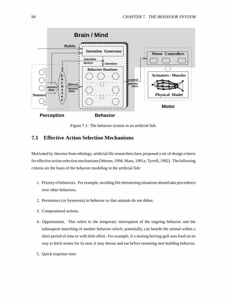
94 CHAPTER 7. THE BEHAVIOR SYSTEM
Motor
Perception Behavior
Motor Controllers
Sensors
filtered
data
eterssensory
Brain / Mind
Behavior Routines
intentionintentiondesires
param-
datasensory
Habits
control
Intention Generator
Actuators / Muscles
Physical Model
Focusser
Figure 7.1: The behavior system in an artificial fish.
7.1 Effective Action Selection Mechanisms
Motivated by theories from ethology, artificial life researchers have proposed a set of design criteria
for effective action selection mechanisms (Werner, 1994; Maes, 1991a; Tyrrell, 1992). The following
criteria are the basis of the behavior modeling in the artificial fish:
1. Priority of behaviors. For example, avoiding life-threatening situations should take precedence
over other behaviors.
2. Persistence (or hysteresis) in behavior so that animals do not dither.
3. Compromised actions.
4. Opportunism. This refers to the temporary interruption of the ongoing behavior and the
subsequent launching of another behavior which, potentially, can benefit the animal within a
short period of time or with little effort. For example, if a nesting herring-gull sees food on its
way to fetch stones for its nest, it may detour and eat before resuming nest building behavior.
5. Quick response time.
7.2. BEHAVIOR CONTROL AND ETHOLOGY 95
7.2 Behavior Control and Ethology
It is often possible to break down complex behavior patterns into smaller units,
some of which are immediately equitable with reflexes. Behavior is frequently
organized in a hierarchical way ... Thus the higher control systems must
compete for control of reflexes rather in the manner that reflexes compete for
control of muscles.
— A. Manning
The behavior control scheme in our artificial animal can be viewed as consisting of two important
relationships. One relationship is between the motor controllers and muscles/fins, and the other
is between some higher control mechanisms and the motor controllers. The motor controllers
coordinate and control the muscles and fins in order to form useful motor skills while, in a similar
manner, higher control mechanisms compete for the control of the motor controllers to generate
meaningful behaviors. This paradigm is consistent with the animal behavior theory proposed by the
ethologist Manning (1979).
In our framework, the higher control mechanisms correspond to the fish’s behavior system, where
the action selection process—the competition over the control of the motor controllers—happens
at two levels: the intention level and the action level. Intentions are governed by the intention
generator and actions are governed by the focusser and the behavior routines. Fig. 7.2 illustrates the
overall control scheme for action selection in the artificial fish.
7.2.1 The Intention Level
At the intention level, different desires compete over what should be done (which desire is to become
the current intention), given the animal’s external and internal conditions. This process can be well
explained by a typical scene generated in our simulation: A fish is heading towards food when it
encounters an obstacle in the way. It makes appropriate turns in order to avoid colliding with the
obstacle, and once the obstacle is cleared it resumes pursuing the food. Such a behavioral sequence
is the result of the competition between the desire to eat food and the desire to avoid collision.
7.2.2 The Action Level
Even when an intention has been decided, it remains to determine how the intention should be
fulfilled through the successive selection of motor actions. The selected sequence of actions, hence
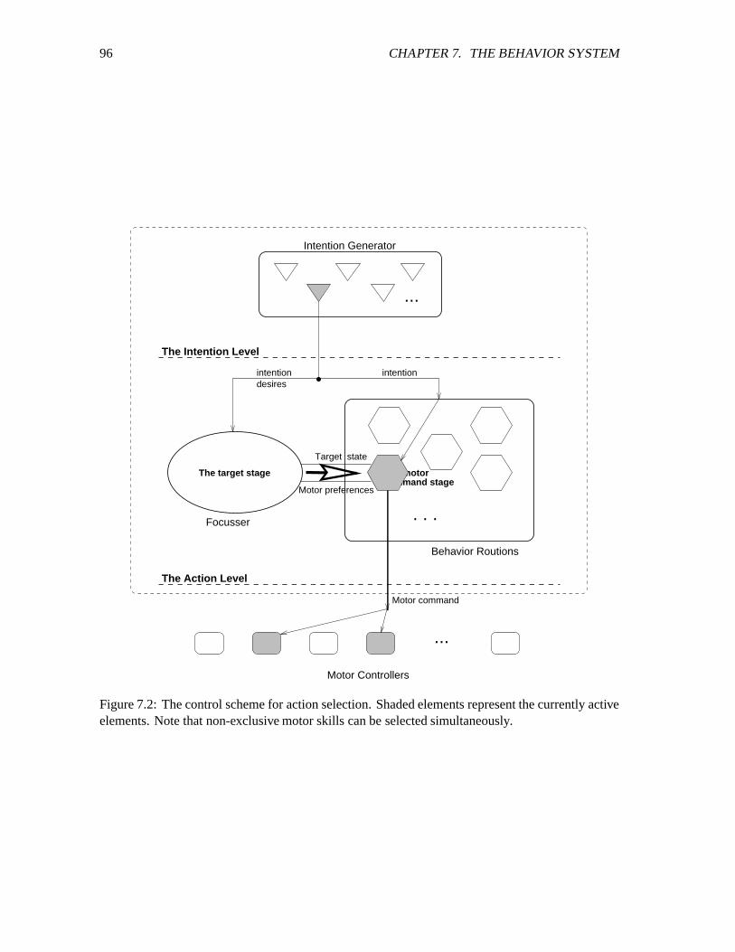
96 CHAPTER 7. THE BEHAVIOR SYSTEM
The Intention Level
The Action Level
Focusser
Intention Generator
...
. . .
Motor Controllers
Behavior Routions
intentionintentiondesires
...
Motor preferences
Target state
Motor command
command stageThe motor The target stage
Figure 7.2: The control scheme for action selection. Shaded elements represent the currently activeelements. Note that non-exclusive motor skills can be selected simultaneously.
7.2. BEHAVIOR CONTROL AND ETHOLOGY 97
the behavioral outcome, depends on the dynamics of the 3D virtual world as well as the dynamics
of the multiple desires of the fish. The latter manifests its effect through the motor preferences
and hence, although there is only one intention or winning behavior at any instant in time, other
behaviors can nonetheless influence the creature’s actions.
We can further analyze the control at this level at two stages—the target stage where the target,
i.e. the object of interest given the current intention, is chosen and the motor command stage where
the final, detailed motor command is calculated. The target stage control is governed by the focusser
and the motor command stage control is governed by the behavior routines.
The control process at the target stage can be viewed as the ‘competition’ amongst the set of
potential targets to become the current target. This is particularly obvious in the cases described in
Section 6.5.3, where the fish tries to decide to which food morsel or mate it should attend. Since
the desirability of each potential target may change over time (due to the dynamics of the virtual
world and the motor preferences), the target may change over time. Consider the case when the fish
intends to eat and there are multiple available food sources; it is possible that a fish may perform an
interesting zigzagging behavior due to the competition between potential targets.
Once the current target is chosen, control is then passed to the active behavior routine. The
final choice of a motor controller and the appropriate control parameters are computed based on the
current state of the fish and the target, as well as the values of the motor preferences (see Section 6.5.3
for examples and details).
7.2.3 Summary
The intricacy of the behaviors we have been able to emulate in the artificial fishes results from the
dynamic interactions between different intentions and between different choices of actions. The
separation of the intention level and the action level in the behavioral control and action selection
scheme makes the design more intuitive and efficient. In particular, since the function of the
intention generator is independent from those of the behavior routines, new behaviors can be added
into the behavior repertoire in steps: First, the behavior routine of a new behavior can be written and
tested independently from the intention generator (and from other behavior routines that are not a
component routine). The intention generator can then be modified to incorporate the new intention
and can also be tested independently.
In the following sections, we describe the implementation of the intention generator, the behavior
98 CHAPTER 7. THE BEHAVIOR SYSTEM
routines, and how they work in conjunction with the perception system to govern effective action
selection in an artificial fish. We start with the fish’s static habits and its dynamic mental state.
7.3 Habits
The animator establishes the innate character of each artificial fish through a set of binary habit
parameters. These parameters determine whether the fish is male or female, and whether it likes,
dislikes, or does not care about
1. brightness,
2. darkness,
3. cold,
4. warmth,
5. schooling.
‘Does not care’ is represented by assigning identical values to the two contradicting habit
parameters. For instance, if both brightness and darkness parameters are assigned ‘1’ or ‘0’ then the
fish does not care about the lighting patterns in its environment.
7.4 Mental State
Unlike a fish’s habits, which are static, its mental state varies over time. The mental state of an
animal can be viewed as consisting of several distinct desires. For example, the desire to drink or
the desire to eat. In order to model an artificial fish’s mental state, it is important to make certain that
the modeled desires resemble the three fundamental properties of natural desires: (a) they should
be time varying; (b) they should depend on either internal urge or external stimuli or both; (c) they
should be satisfiable (see Section 7.4 for more details).
Currently, the artificial fish has three mental state variables, hunger Á , libido  , and fear à .
The range of each variable is %R'�)W*-, , with higher values indicating a stronger desire to eat, mate and
avoid predators, respectively. Á and  are determined both by internal urge and by external sensory
stimuli, while à is solely induced by the latter, i.e., the perception of predators. The variables are
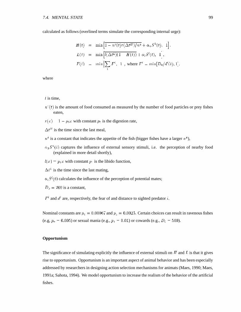
7.4. MENTAL STATE 99
calculated as follows (overlined terms simulate the corresponding internal urge):
Á ��Ä¿�Å0 JÆKNMÈÇ * 6 \ < ��Ä�� ¦ �!ÉLÄ�ÊË� 4 \ : §&ÌUÍ�Î Í ��Ä�� )�*-Ï�) ��Ä¿�Ð0 JÆKNMÈÇ Ñ �!ÉLÄ�Ò �¿� * 6 Á ��Ä¿�¿� §&ÌUÓÔÎ Ó ��Ä�� )�*-Ï�)à ��Ä¿�Ð0 JÆKNM ÇÖÕ T à T )�* Ï ) where à T 0 JLKNMH%(SØ× 4 � T ��Ä�� )+*-,�)
where
Äis time,
\ < ���� is the amount of food consumed as measured by the number of food particles or prey fisheseaten,
¦ � ¡ ��0 * 6�٠׿¡ with constantÙ × is the digestion rate,ÉLÄ Ê
is the time since the last meal,
\ : is a constant that indicates the appetite of the fish (bigger fishes have a larger \ : ),ÌUÍ�Î Í ��Ä�� captures the influence of external sensory stimuli, i.e. the perception of nearby food
(explained in more detail shortly),
Ñ � ¡ ��0�Ù ©´¡ with constantÙ © is the libido function,ÉLÄ Ò
is the time since the last mating,
ÌUÓÔÎ Ó ��Ä�� calculates the influence of the perception of potential mates;
SØ× 0 ¹�'�' is a constant,
à T and � T are, respectively, the fear of and distance to sighted predator X .Nominal constants are
Ù × 0 '�PR''�'�Ú�¼ andÙ © 0 '�PR'�'¹�Q . Certain choices can result in ravenous fishes
(e.g,Ù × 0 '�PR'�'�Q ) or sexual mania (e.g.,
Ù © 0 '�P('�* ) or cowards (e.g., SØ× 0 Q'�' ).
Opportunism
The significance of simulating explicitly the influence of external stimuli on Á and  is that it gives
rise to opportunism. Opportunism is an important aspect of animal behavior and has been especially
addressed by researchers in designing action selection mechanisms for animats (Maes, 1990; Maes,
1991a; Sahota, 1994). We model opportunism to increase the realism of the behavior of the artificial
fishes.
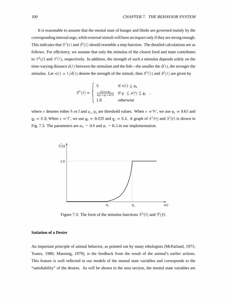
100 CHAPTER 7. THE BEHAVIOR SYSTEM
It is reasonable to assume that the mental state of hunger and libido are governed mainly by the
corresponding internal urge, while external stimuli will have an impact only if they are strong enough.
This indicates that Î Í ��Ä�� and Î Ó ��Ä¿� should resemble a step function. The detailed calculations are as
follows. For efficiency, we assume that only the stimulus of the closest food and mate contributes
to Î Í ��Ä�� and Î Ó ��Ä¿� , respectively. In addition, the strength of such a stimulus depends solely on the
time-varying distance � ��Ä¿� between the stimulant and the fish—the smaller the � ��Ä¿� , the stronger the
stimulus. Let Û ��Ä��10 * 4 � ��Ä¿� denote the strength of the stimuli, then Î Í ��Ä¿� and Î Ó ��Ä¿� are given by
Î�Ü ��Ä¿�j0ÝÞÞÞß ÞÞÞà' if Û ��Ä¿� Y]áW©â�ãÖäNåÔæ�ç�èª çgé´æ�ç�è�æ�â�ãêäNå if áW©�Y[Û ��Ä�� Y]á-ª*�PR' otherwise
)where ¡ denotes either « or Ñ and áW© , á-ª are threshold values. When ¡ 0
‘ « ’, we use áW© 0 '�PR'�Q andá ª 0 '�P(¹ ; When ¡ 0‘ Ñ ’, we use á © 0 '�P('�¹�Q and á ª 0 '�PO* . A graph of Î Í ��Ä¿� and Î Ó ��Ä�� is shown in
Fig. 7.3. The parameters are ÌUÍ 0 '�PR½ and ÌUÓ 0 '�P(Q in our implementation.
1 s(t)2
1.0
q q
S (t)x
Figure 7.3: The form of the stimulus functions Î Í ��Ä�� and Î Ó ��Ä¿� .Satiation of a Desire
An important principle of animal behavior, as pointed out by many ethologists (McFarland, 1971;
Toates, 1980; Manning, 1979), is the feedback from the result of the animal’s earlier actions.
This feature is well reflected in our models of the mental state variables and corresponds to the
“satisfiability” of the desires. As will be shown in the next section, the mental state variables are
7.5. INTENTION GENERATOR 101
directly responsible for activating the matching behaviors. If a behavior is successful, its outcome
should be able to satisfy, albeit perhaps gradually, the desire that triggered the behavior in the first
place. It is essential to model satisfiability, otherwise a behavior may never terminate once activated.
The formulation of the mental state variables exhibits satisfiability as follows: The value of Ãdepends only on the strength of the external stimulus. This means that if the appropriate stimulus
does not exist or is weak, Ã will remain low (or satiated). This can be achieved by two means—first,
the reactive fleeing action of the fish and, second, the dynamic nature of the virtual world. The
values of Á and  are mainly controlled by the corresponding internal urge component whose value
decreases as the result of successful feeding and mating. The external stimulus components, as
we have shown, represent dynamic opportunities and hence are kept at low values under normal
conditions.
Note that in the formulation of Á , the internal urge component restrains the stimulus component
such that the fish will not keep taking opportunities to eat food (even when opportunities keep
presenting themselves) to the exclusion of all other behaviors. For example, once the amount of
food taken \ < exceeds twice the value of the fish’s appetite \ : , then Á becomes zero. This situation
continues until ¦ �!ÉLÄ Ê � Y�' indicating the complete digestion of the food, at which moment, \ < is
reset to zero.
7.5 Intention Generator
Fig. 7.4 illustrates a simplified generic intention generator which is responsible for the goal-directed
behavior of the artificial fish in its dynamic world.
The intention generator is based on a priority hierarchy of behaviors. Life threatening behaviors,
such as collision avoidance, have highest priority. As indicated in the figure, the intention generator
first checks the sensory information stream to see if there is any immediate danger of collision. If
there is (see Chapter 6 for collision test) then the intention ë generated is to avoid collision. If there is
no immediate danger of collision, the neighborhood is searched for predators, the fear state variableà and the most dangerous predator ì for which à .dí à T (for any predator X ) are calculated. If
the total fear Ãxî�¤�× (where '�PO*LY�¤�×ïY�'�P(Q is a threshold value) evasive action is to be taken. If
the most dangerous predator is not too threatening (i.e. à .�𠤩 where ¤©�îu¤{× ) and the fish has a
schooling habit, then the school intention is generated, otherwise the escape intention is generated.
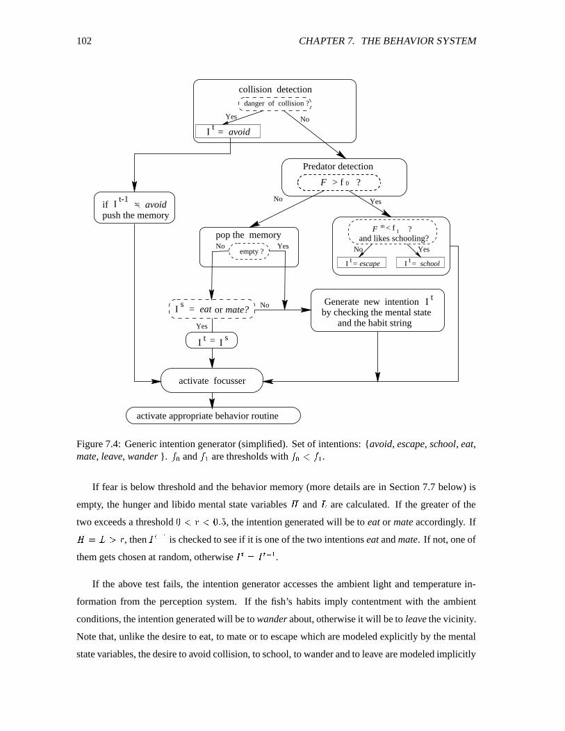
102 CHAPTER 7. THE BEHAVIOR SYSTEM
Predator detection
NoYes
danger of collision ?
collision detection
Yes
mate?or= eat
= escape
by checking the mental state
activate appropriate behavior routine
activate focusser
=
Generate new intention
and the habit string
t
?m
and likes schooling?YesNo
F
I
Yes
No
No
< f
s
I t
II
I t-1
I s
t
I
= avoidtI
1
t
F > f ?0
= school
=push the memory
avoidif
empty ?No
pop the memoryYes
Figure 7.4: Generic intention generator (simplified). Set of intentions: {avoid, escape, school, eat,mate, leave, wander }. ¤�× and ¤© are thresholds with ¤�× ð ¤© .
If fear is below threshold and the behavior memory (more details are in Section 7.7 below) is
empty, the hunger and libido mental state variables Á and  are calculated. If the greater of the
two exceeds a threshold ' ð ¦ ð ' PRQ , the intention generated will be to eat or mate accordingly. IfÁ 0 Â]î[¦ , then ë ägæ © is checked to see if it is one of the two intentions eat and mate. If not, one of
them gets chosen at random, otherwise ë ä 0 ë äñæ © .If the above test fails, the intention generator accesses the ambient light and temperature in-
formation from the perception system. If the fish’s habits imply contentment with the ambient
conditions, the intention generated will be to wander about, otherwise it will be to leave the vicinity.
Note that, unlike the desire to eat, to mate or to escape which are modeled explicitly by the mental
state variables, the desire to avoid collision, to school, to wander and to leave are modeled implicitly
7.5. INTENTION GENERATOR 103
by their intrinsic behavioral priorities (level in the hierarchy), sensory stimuli and innate habits. The
following diagram shows all the desires ordered according to their levels in the priority hierarchy:
Desire to avoid collisionòDesire to flee from predatorò
Desire to eat, Desire to mateòDesire to schoolò
Desire to wander, Desire to leave
7.5.1 Why Hierarchy?
Ethological Background
Ethologists have long believed that the control of action selection in animals is hierarchical in
structure (Lorenz, 1981; Tinbergen, 1951; Dawkins, 1976). This classical view is supported by
extensive observation of and numerous experiments on animal behavior. Tinbergen (1951) described
a “working hypothesis” of an action selection mechanism composed of a hierarchy of nodes. The
top level nodes represent high-level motivational behaviors, such as “reproduction”. The lowest
level nodes correspond to simple sub-behaviors such as “lay eggs” and “comb feathers”. There is
a feeding of activation down through the hierarchy. Nodes in the same level inhibit one another so
that only one can be active at any time. Lorenz (1981) described a similar idea which emphasizes
the effect of both internal and external stimuli in activating a specific behavior.
Implementation Advantages
Using a hierarchy to implement behavior arbitration offers certain advantages:
Handling Complexity and Conflict: Hierarchical structures are highly intuitive and hence easier
to design and to diagnose. Very complex systems can be put together in a modular fashion.
104 CHAPTER 7. THE BEHAVIOR SYSTEM
Additionally, in a hierarchy of behaviors, conflicts between them are greatly reduced by the
more or less fixed priority preferences inherited in the structure.
Increasing Efficiency: Efficiency is obtained by information sharing. Knowledge obtained or pro-
cessed by behaviors higher in the hierarchy can be used by behaviors lower in the hierarchy.
For example, in the intention generator, when control flows down to the behavior ‘eating’,
previously processed sensory information about surrounding obstacles (by the ‘avoiding ob-
stacle’ behavior) can be used when the focusser is activated to compute the motor preferences
(see the next section or Section 6.5.2) for performing the eating behavior.
Compared with distributed control structures, hierarchical control structures offer lower flexibility
but higher controllability. In particular, hierarchical control involves a much smaller number of
control parameters and hence makes it easy to converge to a desirable choice, while this is not
necessarily true for distributed control.
7.6 Intention-Guided Perception: Control of the Focusser
As is described in the previous chapter, after the intention generator chooses an intention, it invokes
the focusser. For example, when the avoid intention is generated, the perception focusser is activated
to locate the positions of the obstacles, paying special attention to the most dangerous one. To enable
the choice of favorable actions, the focusser must compute motor preferences in accordance with
the environmental conditions (see Section. 6.5.3 for details). This process requires the availability
of " —the strength of the desire from which a motor preference was assigned a value. In the current
implementation, motor preferences may be derived from four desires: avoid (collision), fear, eat and
mate. Let " : , " / , " < and " . denote the strength of these four desires, respectively. Their values are
given by:
" : 0 *�PR'�)" / 0 Ã 4 "�ó�)" < 0 Á 4 " ó )" . 0 Â 4 " ó )
where " ó ( ë 0 ·{ô )öõ�)ö¤�)öì$¸ ) is the strength of the current intention and if ë�÷0 ·{ô )ºõ )º¤ )ºì$¸ , " ó 0 *PR' .
7.7. PERSISTENCE IN BEHAVIOR 105
Once the focusser has computed and collected all the motor preferences, it passes only in-
formation about the geometry, positions, and/or velocities of the attended object along with these
preferences to the appropriate behavior routine.
7.7 Persistence in Behavior
In a complex dynamic world, an artificial fish should have some persistence in its behavior, especially
in its intentions, otherwise it will tend to dither, perpetually changing its mind. Basic persistence
in the behaviors is modeled implicitly by the intrinsic ranking (prioritization) between them, the
continuity in the mental state variables, and the constancy of the habits. For instance, the collision
avoidance behavior precedes all other behaviors and once invoked, will only terminate when the
collision is cleared. Once the mental state of hunger is high enough to activate the feeding behavior,
the continuity in Á (in particular the internal urge component) ensures that the activation level will
not drop abruptly until the fish succeeds in taking more food. However, special attention needs
to be paid to the maintenance of persistence in the case when an ongoing behavior is interrupted
temporarily. In our case, there are two possible situations where an ongoing behavior may be
interrupted: it may be interrupted by a behavior higher in the priority hierarchy triggered by some
event or by an opportunity-triggered behavior.
7.7.1 Behavior Memory
If the current behavior is interrupted, the intention generator is able to store in a single-item short term
memory (we do not wish to give artificial fish an unnaturally large memory capacity) the current
intention and some associated information that may be used to resume the interrupted behavior.
The typical use of this behavior memory is illustrated in Fig. 7.4. The persistence serves mainly
to make longer duration behaviors such as feeding, mating and schooling more robust. Suppose
for example that the current behavior is mating and that an imminent collision is detected. This
causes an avoid intention and the storage of the mate intention (we refer to the stored intention
as ë â in Fig. 7.4) along with the identity of the mating partner. After the obstacle is cleared, the
intention generator commands the focusser to generate up-to-date heading and range information
about the mating partner, assuming it is still in viewing range. A similar scenario may occur during
feeding. Moreover, feeding and mating can interrupt one another if appropriate opportunities present
themselves.
106 CHAPTER 7. THE BEHAVIOR SYSTEM
7.7.2 Inhibitory Gain and Fatigue
To further ensure persistence in a behavior that has been interrupted and then resumed, we adopt
the concept of inhibitory gain from ethology (Ludlow, 1980). Inhibitory gain was first proposed
by Ludlow to model the control mechanism in animals that balances persistence and opportunism.
It is elicited by the winning behavior and is a negative value imposed on the activation energy
(strength of desire) of all the competing behaviors. This helps to keep the activation of the winning
behavior relatively high and hence induces persistence in that behavior. The higher the value of the
inhibitory gain, the more persistent the behavior that releases it. In our case, since behaviors are
layered in a hierarchy by their intrinsic priorities, the number of competing behaviors is reduced
to those in the same layer rather than to all of the other behaviors had a distributed structure been
used. The inhibitory gain ø 0|6 '�PR¹�" (where " is the activation value of the active behavior) is
added to the competing behaviors only when the current behavior is one resumed from the behavior
memory. Let us take the same example as above. When the mating behavior is resumed from
the obstacle avoidance behavior, ø is added to Á to help maintain the persistence/continuity of the
mating behavior by inhibiting further interruptions, say, from opportunistic feeding.
Excessive persistence in behavior can be undesirable in certain situations. For example, if we
do not put food in the virtual marine world, a hungry fish would not engage in any behavior (in
the same or lower priority layer) other than foraging. This can be avoided by modeling fatigue in
behavior. Fatigue is also important for behavior time-sharing (McFarland, 1993a), in which low
priority activities are given a chance to execute despite the presence of a higher priority activity.
We model fatigue of a behavior by simply multiplying the corresponding activation value of that
behavior with a decay function of time. A similar model of inhibitory gain and fatigue was proposed
by Blumberg (1994).
7.7.3 Persistence in Targeting
Different persistence can also be exhibited in the way an animal chooses its targets over time. Our
design of the intention generator and focusser simplifies the modification of existing personalities
and behaviors and the addition of new ones. For example, we can create artificial fishes with
different persistences by augmenting the focusser with a positive valued threshold. Suppose the
current intention of a predator fish is to eat and let the distance to some currently targeted prey be ÑÔùand the distance to some other prey be ÑOú . If Ñ ù 6 Ñûú is greater than the threshold, the fish will target
7.8. BEHAVIOR ROUTINES 107
the new prey. Varying the threshold will vary the fish’s level of persistence. The same heuristic can
be applied to mates when the fish is trying to mate. One can make the fish “fickle” by setting the
value of the threshold close to zero or make it “devoted” by setting a large value.
7.8 Behavior Routines
Once the intention generator selects an intention, it attempts to satisfy the intention by passing
control to a behavior routine along with the data from the perception focusser. The artificial fish
currently includes nine behavior routines listed below plus five subroutines (listed within brackets
below) which serve the obvious purposes:
1. avoiding-static-obstacle
2. avoiding-fish
3. chasing-target
4. eating-food (suck-in)
5. mating (looping, circling, ascending, nuzzling)
6. leaving
7. wandering
8. escaping
9. schooling
The activated behavior routine uses the focused perceptual data to select appropriate MCs and
provide them with the proper motor control parameters. Note that more than one MC may be
chosen if they are not mutually exclusive. For instance, i �F>º�HC ��� and p i ��qWE ®�C ��� can be selected
simultaneously. We now briefly describe the function of the routines.
The avoiding-static-obstacleand avoiding-fish routines enable a fish to avoid potential collisions.
The chasing-target routine guides a fish as it swims towards a goal. These more primitive, perception-
driven behaviors are essential components of the more advanced motivational behaviors such as
preying, schooling, and mating. We will give a more detailed description of these behaviors in the
subsequent section.
The eating-food routine tests the distance � from the fish’s mouth to the targeted food (see
Fig. 7.6). If � is greater than some small threshold value, the routine chasing-target is invoked.
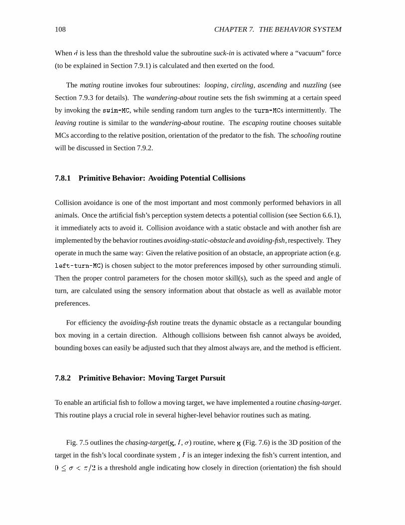
108 CHAPTER 7. THE BEHAVIOR SYSTEM
When � is less than the threshold value the subroutine suck-in is activated where a “vacuum” force
(to be explained in Section 7.9.1) is calculated and then exerted on the food.
The mating routine invokes four subroutines: looping, circling, ascending and nuzzling (see
Section 7.9.3 for details). The wandering-about routine sets the fish swimming at a certain speed
by invoking the i �?>ö�fC ��� , while sending random turn angles to the BD�=�E?C ��� s intermittently. The
leaving routine is similar to the wandering-about routine. The escaping routine chooses suitable
MCs according to the relative position, orientation of the predator to the fish. The schooling routine
will be discussed in Section 7.9.2.
7.8.1 Primitive Behavior: Avoiding Potential Collisions
Collision avoidance is one of the most important and most commonly performed behaviors in all
animals. Once the artificial fish’s perception system detects a potential collision (see Section 6.6.1),
it immediately acts to avoid it. Collision avoidance with a static obstacle and with another fish are
implemented by the behavior routines avoiding-static-obstacle and avoiding-fish, respectively. They
operate in much the same way: Given the relative position of an obstacle, an appropriate action (e.g.r q ^ B C�BD�=EFC ��� ) is chosen subject to the motor preferences imposed by other surrounding stimuli.
Then the proper control parameters for the chosen motor skill(s), such as the speed and angle of
turn, are calculated using the sensory information about that obstacle as well as available motor
preferences.
For efficiency the avoiding-fish routine treats the dynamic obstacle as a rectangular bounding
box moving in a certain direction. Although collisions between fish cannot always be avoided,
bounding boxes can easily be adjusted such that they almost always are, and the method is efficient.
7.8.2 Primitive Behavior: Moving Target Pursuit
To enable an artificial fish to follow a moving target, we have implemented a routine chasing-target.
This routine plays a crucial role in several higher-level behavior routines such as mating.
Fig. 7.5 outlines the chasing-target( ü , ë , ý ) routine, where ü (Fig. 7.6) is the 3D position of the
target in the fish’s local coordinate system , ë is an integer indexing the fish’s current intention, and'�Y±ý ð±þU4 ¹ is a threshold angle indicating how closely in direction (orientation) the fish should
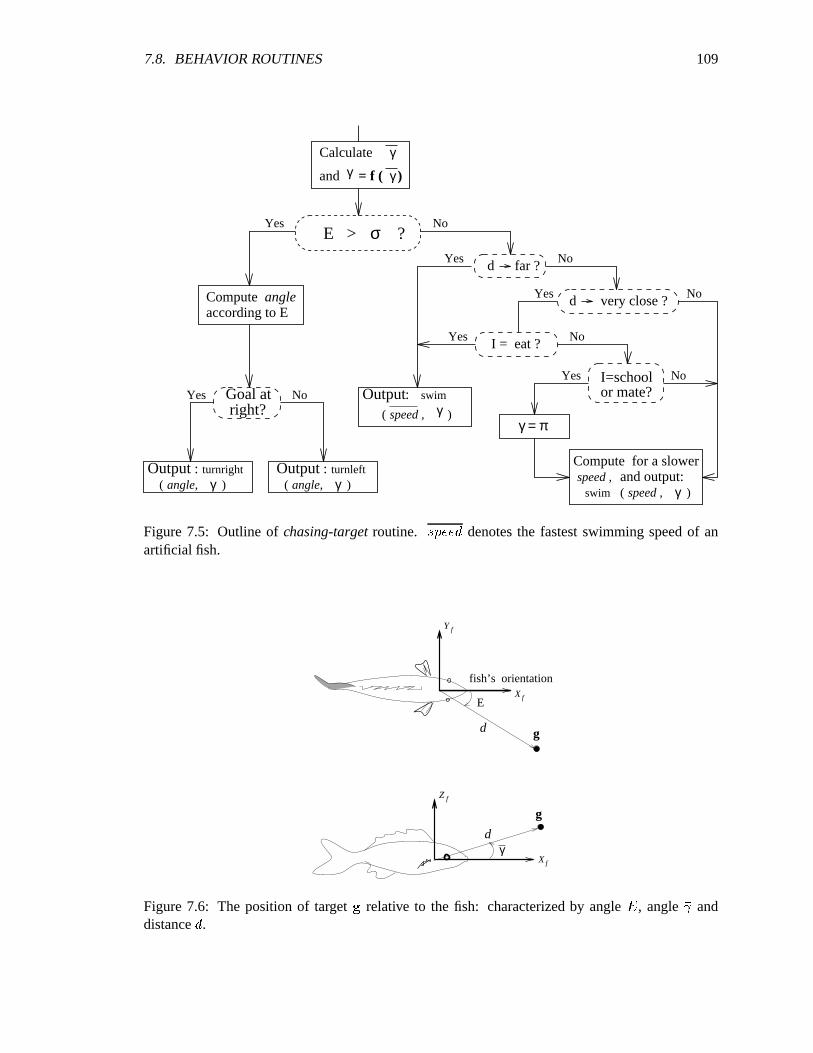
7.8. BEHAVIOR ROUTINES 109
or mate?Yes No
E > ?Yes No
Goal atright?
Yes
d
far ?d
very close ?Yes
I=school
No
I = eat ?Yes No
NoYes
No
σ
Calculate
and = f ( )
γγ γ
Output : turnright Output : turnleft
Output:
γ = π
Compute angleaccording to E
angle, γ angle, γ
speed , γ
Compute for a slowerspeed , and output:
speed , γ( ) ( )
( )
swim
swim ( )
Figure 7.5: Outline of chasing-target routine. ÿ�������� denotes the fastest swimming speed of anartificial fish.
Y
d
d
E
f
g
gfZ
fish’s orientation
f
γ
X f
X
Figure 7.6: The position of target � relative to the fish: characterized by angle � , angle anddistance � .
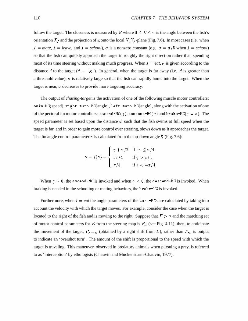
110 CHAPTER 7. THE BEHAVIOR SYSTEM
follow the target. The closeness is measured by � where � ������� is the angle between the fish’s
orientation ��� and the projection of � onto the local ������� -plane (Fig. 7.6). In most cases (i.e. when���mate,
���leave, and
���school), � is a nonzero constant (e.g. � � ����� when
���school)
so that the fish can quickly approach the target in roughly the right direction rather than spending
most of its time steering without making much progress. When���
eat, � is given according to the
distance � to the target ( � � �!� � �!� ). In general, when the target is far away (i.e. � is greater than
a threshold value), � is relatively large so that the fish can rapidly home into the target. When the
target is near, � decreases to provide more targeting accuracy.
The output of chasing-target is the activation of one of the following muscle motor controllers:i#"%$'&)(#*,+.- speed / , 0 $�132546(�437 098 (�*,+3- angle / , :<;�= 46(�437 038 (�*,+3- angle / , along with the activation of one
of the pectoral fin motor controllers: > i@? ;�8�A (�*,+,-B / , A<; i.? ;�8�A (#*,+,-C / and D,06>�E6; (#*,+,-C � �F/ . The
speed parameter is set based upon the distance � , such that the fish swims at full speed when the
target is far, and in order to gain more control over steering, slows down as it approaches the target.
The fin angle control parameter is calculated from the up-down angle (Fig. 7.6):
�HG - / �IJJJK JJJL M ����N if
� � ���F��OP ����O if RQ �F��O����O if RSUT �F��O
When VQ � , the > i@? ;�8<A (�*,+ is invoked and when VS � , the A<; i@? ;�8�A (�*,+ is invoked. When
braking is needed in the schooling or mating behaviors, the D,06>�E6; (#*,+ is invoked.
Furthermore, when�W�
eat the angle parameters of the 497 038 (#*5+ s are calculated by taking into
account the velocity with which the target moves. For example, consider the case when the target is
located to the right of the fish and is moving to the right. Suppose that � Q � and the matching set
of motor control parameters for � from the steering map is XZY (see Fig. 4.11), then, to anticipate
the movement of the target, X Y\[,]^Y (obtained by a right shift from � ), rather than X Y , is output
to indicate an ‘overshot turn’. The amount of the shift is proportional to the speed with which the
target is traveling. This maneuver, observed in predatory animals when pursuing a prey, is referred
to as ‘interception’ by ethologists (Chauvin and Muckensturm-Chauvin, 1977).

7.8. BEHAVIOR ROUTINES 111
Figure 7.7: A peaceful marine world. See the original color image in Appendix D.
Figure 7.8: The smell of danger. See the original color image in Appendix D.
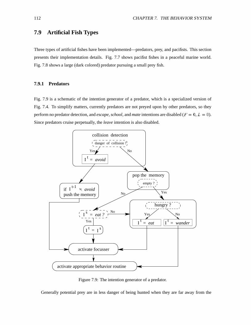
112 CHAPTER 7. THE BEHAVIOR SYSTEM
7.9 Artificial Fish Types
Three types of artificial fishes have been implemented—predators, prey, and pacifists. This section
presents their implementation details. Fig. 7.7 shows pacifist fishes in a peaceful marine world.
Fig. 7.8 shows a large (dark colored) predator pursuing a small prey fish.
7.9.1 Predators
Fig. 7.9 is a schematic of the intention generator of a predator, which is a specialized version of
Fig. 7.4. To simplify matters, currently predators are not preyed upon by other predators, so they
perform no predator detection, and escape, school, and mate intentions are disabled ( _ � � , ` � � ).Since predators cruise perpetually, the leave intention is also disabled.
YesNo
No
No
Yes
activate focusser
activate appropriate behavior routine
Yes
collision detection
hungry ?
NoYes
I t= eat
I t= avoid
t-1
= wander
danger of collision ?
empty ?
tI
pop the memory
I
t =
I s= eat ?
I
=if avoid
sI
push the memory
Figure 7.9: The intention generator of a predator.
Generally potential prey are in less danger of being hunted when they are far away from the
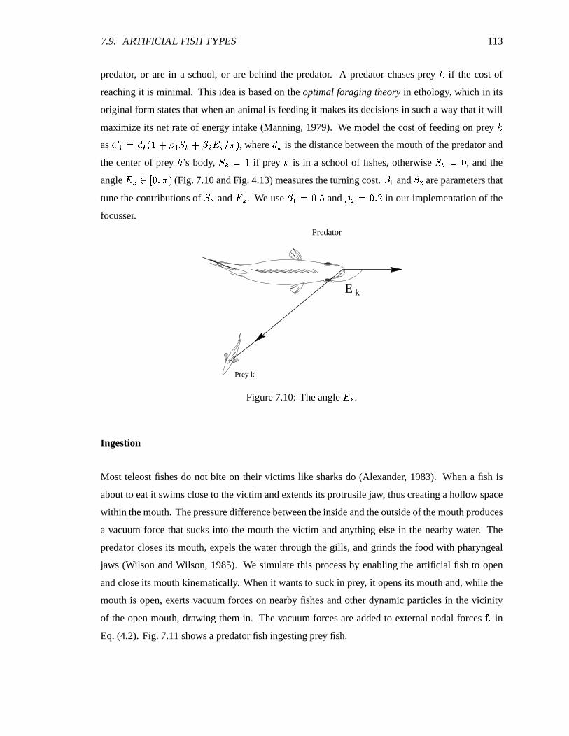
7.9. ARTIFICIAL FISH TYPES 113
predator, or are in a school, or are behind the predator. A predator chases prey a if the cost of
reaching it is minimal. This idea is based on the optimal foraging theory in ethology, which in its
original form states that when an animal is feeding it makes its decisions in such a way that it will
maximize its net rate of energy intake (Manning, 1979). We model the cost of feeding on prey aas bdc � �.c -fedMVgZh�i c MVg%j �kc����F/ , where �.c is the distance between the mouth of the predator and
the center of prey a ’s body, i c � e if prey a is in a school of fishes, otherwise i c � � , and the
angle �kcmlonp�,qf�F/ (Fig. 7.10 and Fig. 4.13) measures the turning cost. g)h and g\j are parameters that
tune the contributions of i c and �kc . We use g)h � �,rp� and g\j � �,rsN in our implementation of the
focusser.
Prey k
Predator
E k
Figure 7.10: The angle �tc .
Ingestion
Most teleost fishes do not bite on their victims like sharks do (Alexander, 1983). When a fish is
about to eat it swims close to the victim and extends its protrusile jaw, thus creating a hollow space
within the mouth. The pressure difference between the inside and the outside of the mouth produces
a vacuum force that sucks into the mouth the victim and anything else in the nearby water. The
predator closes its mouth, expels the water through the gills, and grinds the food with pharyngeal
jaws (Wilson and Wilson, 1985). We simulate this process by enabling the artificial fish to open
and close its mouth kinematically. When it wants to suck in prey, it opens its mouth and, while the
mouth is open, exerts vacuum forces on nearby fishes and other dynamic particles in the vicinity
of the open mouth, drawing them in. The vacuum forces are added to external nodal forces uCv in
Eq. (4.2). Fig. 7.11 shows a predator fish ingesting prey fish.
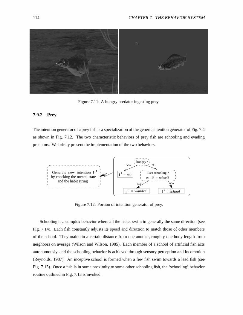
114 CHAPTER 7. THE BEHAVIOR SYSTEM
Figure 7.11: A hungry predator ingesting prey.
7.9.2 Prey
The intention generator of a prey fish is a specialization of the generic intention generator of Fig. 7.4
as shown in Fig. 7.12. The two characteristic behaviors of prey fish are schooling and evading
predators. We briefly present the implementation of the two behaviors.
hungry?
likes schooling ?
I t = wander
NoYes
No Yes
= schooltI
t
by checking the mental stateand the habit string
Generate new intention I= eat
= school?orI t
sI
Figure 7.12: Portion of intention generator of prey.
Schooling is a complex behavior where all the fishes swim in generally the same direction (see
Fig. 7.14). Each fish constantly adjusts its speed and direction to match those of other members
of the school. They maintain a certain distance from one another, roughly one body length from
neighbors on average (Wilson and Wilson, 1985). Each member of a school of artificial fish acts
autonomously, and the schooling behavior is achieved through sensory perception and locomotion
(Reynolds, 1987). An inceptive school is formed when a few fish swim towards a lead fish (see
Fig. 7.15). Once a fish is in some proximity to some other schooling fish, the ‘schooling’ behavior
routine outlined in Fig. 7.13 is invoked.
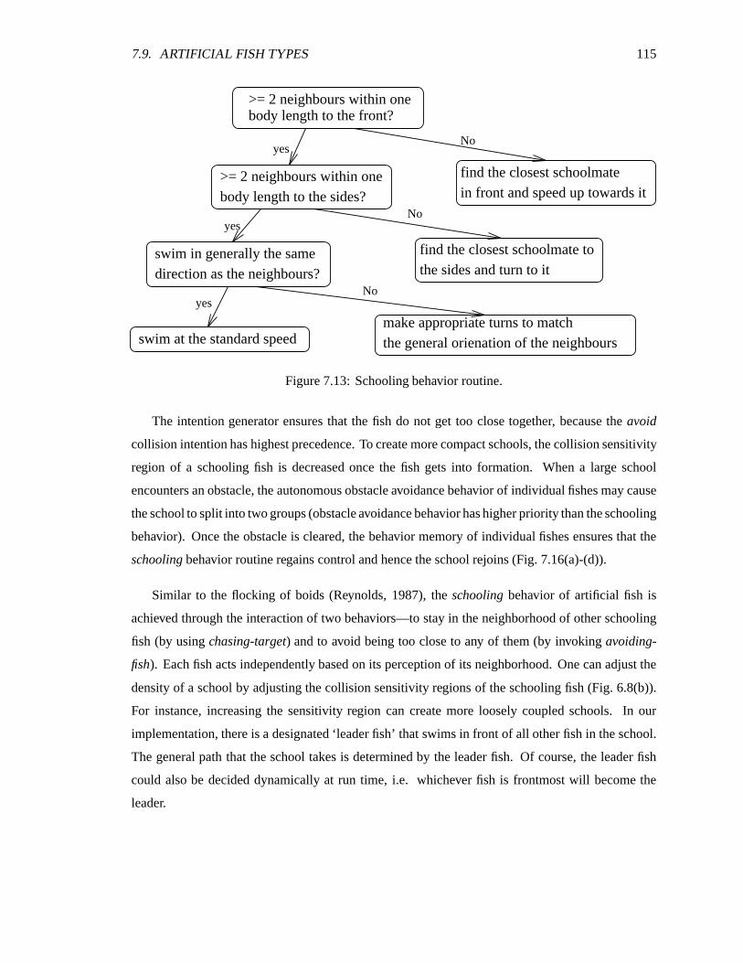
7.9. ARTIFICIAL FISH TYPES 115
>= 2 neighbours within one body length to the front?
find the closest schoolmate in front and speed up towards it
swim in generally the samedirection as the neighbours?
yesNo
yes
yes
No
No
swim at the standard speed
body length to the sides?
the sides and turn to it
make appropriate turns to matchthe general orienation of the neighbours
find the closest schoolmate to
>= 2 neighbours within one
Figure 7.13: Schooling behavior routine.
The intention generator ensures that the fish do not get too close together, because the avoid
collision intention has highest precedence. To create more compact schools, the collision sensitivity
region of a schooling fish is decreased once the fish gets into formation. When a large school
encounters an obstacle, the autonomous obstacle avoidance behavior of individual fishes may cause
the school to split into two groups (obstacle avoidance behavior has higher priority than the schooling
behavior). Once the obstacle is cleared, the behavior memory of individual fishes ensures that the
schooling behavior routine regains control and hence the school rejoins (Fig. 7.16(a)-(d)).
Similar to the flocking of boids (Reynolds, 1987), the schooling behavior of artificial fish is
achieved through the interaction of two behaviors—to stay in the neighborhood of other schooling
fish (by using chasing-target) and to avoid being too close to any of them (by invoking avoiding-
fish). Each fish acts independently based on its perception of its neighborhood. One can adjust the
density of a school by adjusting the collision sensitivity regions of the schooling fish (Fig. 6.8(b)).
For instance, increasing the sensitivity region can create more loosely coupled schools. In our
implementation, there is a designated ‘leader fish’ that swims in front of all other fish in the school.
The general path that the school takes is determined by the leader fish. Of course, the leader fish
could also be decided dynamically at run time, i.e. whichever fish is frontmost will become the
leader.
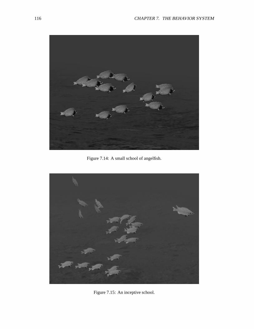
116 CHAPTER 7. THE BEHAVIOR SYSTEM
Figure 7.14: A small school of angelfish.
Figure 7.15: An inceptive school.
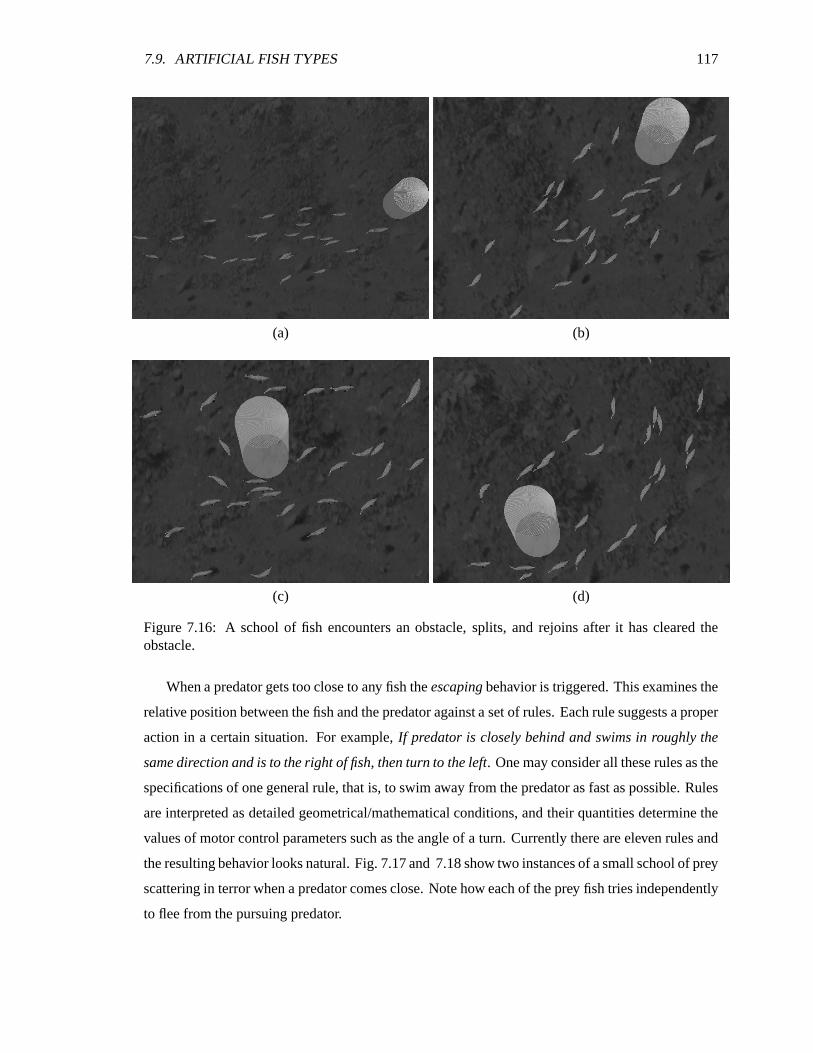
7.9. ARTIFICIAL FISH TYPES 117
(a) (b)
(c) (d)
Figure 7.16: A school of fish encounters an obstacle, splits, and rejoins after it has cleared theobstacle.
When a predator gets too close to any fish the escaping behavior is triggered. This examines the
relative position between the fish and the predator against a set of rules. Each rule suggests a proper
action in a certain situation. For example, If predator is closely behind and swims in roughly the
same direction and is to the right of fish, then turn to the left. One may consider all these rules as the
specifications of one general rule, that is, to swim away from the predator as fast as possible. Rules
are interpreted as detailed geometrical/mathematical conditions, and their quantities determine the
values of motor control parameters such as the angle of a turn. Currently there are eleven rules and
the resulting behavior looks natural. Fig. 7.17 and 7.18 show two instances of a small school of prey
scattering in terror when a predator comes close. Note how each of the prey fish tries independently
to flee from the pursuing predator.
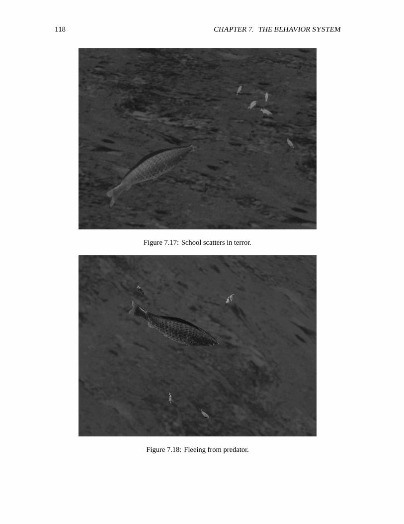
118 CHAPTER 7. THE BEHAVIOR SYSTEM
Figure 7.17: School scatters in terror.
Figure 7.18: Fleeing from predator.
7.9. ARTIFICIAL FISH TYPES 119
The eleven rules based on which a prey fish flees from a predator are listed below (note “me” or
“mine” indicate the fleeing prey fish):
if predator is far:
– if predator is in front, then turn 180 degrees;
– else if predator is behind, then swim forward at full speed;
– else if predator is to the left side, then turn right;
– else if predator is to the right side, then turn left;
if predator is close:
w If predator is in front:
– if predator’s heading is roughly perpendicular to mine, then:x if predator is heading towards my left side, then turn right;x else turn left;
– else turn 180 degrees;
w Else if predator is behind:
– if predator’s heading is roughly the same as mine and is approaching, then:x if predator is to the left, then turn right;x else turn left;
– else if predator’s heading is roughly perpendicular to mine, then:x if predator is heading towards my left side, then turn right;x else turn left;
– else swim forward at full speed;
w Else if predator is to the side:
– if predator is to the left, then turn right;
– else turn left;
7.9.3 Pacifists
The intention generator of a pacifist differs from that of a prey in that intention mate is enabled and
the intentions escape and school are disabled. Piscatorial mating behaviors show great interspecies
and intra-species diversity (Thresher, 1984). However, two behaviors are prevalent: (i) nuzzling,
where typically the male approaches the female from underneath and nudges her abdomen repeatedly
until she is ready to spawn, and (ii) spawning ascent, where in its simplest form, the female rapidly
120 CHAPTER 7. THE BEHAVIOR SYSTEM
swims towards the surface pursued by the male and releases gametes at the peak of her ascent.
Moreover, courtship dancing is common in many species, albeit with substantial variation. Two
frequently observed patterns are looping, in which the male swims vigorously up and down in a
loop slightly above and in front of the female, and circling, in which the male and female circle,
seemingly chasing each other’s tail. Fig. 7.19 shows photographs of natural fish displaying various
mating behaviors (Thresher, 1984).
The complex mating rituals observed in the majority of animals are composed of a sequence of
sub-behaviors (e.g. courting, spawning ascent) performed in a unique order. This is referred to as
fixed action patterns by ethologists (Tinbergen, 1951). We have implemented a mating behavior
routine which simulates courtship looping, circling, spawning ascent, and nuzzling in sequence (see
Fig. 7.20 and Fig. 7.9.3(a)-(f)). This sequence is represented as a finite-state machine where each
state is linked with a component behavior and has a boolean transition function. The transition
function evaluates the associated behavior to see if it is completed, if positive, a transition is
performed and the next component behavior is activated.
A male fish selects a mating partner based on the following criteria: A female of the same species
is more attractive than one of different species, and closer females are more attractive than ones
further away. A female selects a partner similarly, but shows preference to male fish size (stronger,
more protective) rather than proximity. Suppose some fish y has selected a potential partner z then
one of three things may happen:
Fish z ’s intention is not to mate: Fish y approaches z and follows it around by performing the
chasing-target behavior.
Fish z ’s intention is to mate but not with fish y : If y is female it will choose another potential
mate. Otherwise y is male and it will perform looping behavior in front of z for a certain
amount of time. If z is suitably impressed during this time period then she will select y and
the courtship sequence continues, otherwise y will discontinue looping and leave z to find a
new potential partner. Fig. 7.20 shows two examples where two male poker fish vying for the
attention of a female by performing elaborate looping behavior.
Fish z ’s intention is to mate with fish y : Courtship behavior starts with the male looping in front
of the female while she hovers and bobs her head. The female’s hovering and head bobbing
is accomplished through motor control of her pectoral fins.
The male looping behavior is simulated by invoking chasing-target, with the ‘target’ being a
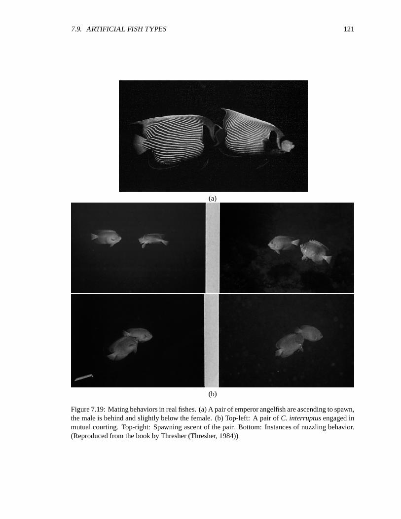
7.9. ARTIFICIAL FISH TYPES 121
(a)
(b)
Figure 7.19: Mating behaviors in real fishes. (a) A pair of emperor angelfish are ascending to spawn,the male is behind and slightly below the female. (b) Top-left: A pair of C. interruptus engaged inmutual courting. Top-right: Spawning ascent of the pair. Bottom: Instances of nuzzling behavior.(Reproduced from the book by Thresher (Thresher, 1984))
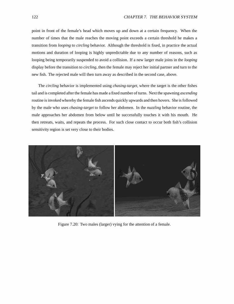
122 CHAPTER 7. THE BEHAVIOR SYSTEM
point in front of the female’s head which moves up and down at a certain frequency. When the
number of times that the male reaches the moving point exceeds a certain threshold he makes a
transition from looping to circling behavior. Although the threshold is fixed, in practice the actual
motions and duration of looping is highly unpredictable due to any number of reasons, such as
looping being temporarily suspended to avoid a collision. If a new larger male joins in the looping
display before the transition to circling, then the female may reject her initial partner and turn to the
new fish. The rejected male will then turn away as described in the second case, above.
The circling behavior is implemented using chasing-target, where the target is the other fishes
tail and is completed after the female has made a fixed number of turns. Next the spawning ascending
routine is invoked whereby the female fish ascends quickly upwards and then hovers. She is followed
by the male who uses chasing-target to follow her abdomen. In the nuzzling behavior routine, the
male approaches her abdomen from below until he successfully touches it with his mouth. He
then retreats, waits, and repeats the process. For such close contact to occur both fish’s collision
sensitivity region is set very close to their bodies.
Figure 7.20: Two males (larger) vying for the attention of a female.
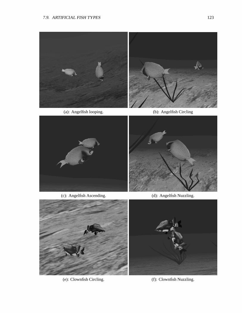
7.9. ARTIFICIAL FISH TYPES 123
(a): Angelfish looping. (b): Angelfish Circling
(c): Angelfish Ascending. (d): Angelfish Nuzzling.
(e): Clownfish Circling. (f): Clownfish Nuzzling.
124 CHAPTER 7. THE BEHAVIOR SYSTEM
7.10 Discussion
In this section we examine the properties of our action selection mechanism against a set of cri-
teria commonly accepted by researchers in designing animats. Possible extensions of our current
implementation are also discussed.
7.10.1 Analysis
The set of design criteria for effective action selection mechanisms listed in the beginning of this
chapter can also be used to evaluate the effectiveness of an action selection mechanism. Next, we
examine the properties of our design of the artificial fish’s behavior system against each of those
criteria and present the result.
Priority of Different Behaviors
The priorities of the range of behaviors we have emulated are implemented by the hierarchical
structure of the intention generator. Life-preserving behaviors (collision avoidance, escape from
predators) are guaranteed to take precedence over other behaviors. Behaviors at the same priority
level in the hierarchy, such as eating and mating, are further prioritized by the dynamics of the
corresponding desires.
Persistence in Behavior
Persistence in behavior is achieved by the use of the simple memory, and the modeling of inhibitory
gain and fatigue described in Section 7.7.
Compromised Actions
Compromised actions are enabled in the behavior system via the use of motor preferences. This
design is considerably more efficient than that of a free-flow hierarchy (Tyrrell, 1993b). In a free-
flow hierarchy, every behavior must compute a recommendation for the next action. There will be no
winner until all of the recommendations arrive at the motor command level, where a winning action
is decided by fusing all the recommendations (see Appendix C.2 for more detail about free-flow
7.10. DISCUSSION 125
hierarchy). While a free-flow hierarchy pays no special attention to the most desirable behavior
given the current situation, our design of the intention generator takes the opposite approach. It picks
a winning behavior at an early stage such that irrelevant sensory information need not be processed.
This reflects the advantages of a winner-takes-all selection process. However, unlike a conventional
winner-takes-all process, the use of the motor preferences allows unselected behaviors to influence
how the winning behavior is performed. We believe that our implementation is a good compromise
between efficiency and functionality.
Moreover, the qualitative nature of the motor preferences simplifies both the process of generating
them and the way of using them (see Section 6.5.3). This is in direct contrast to the quantitative
action recommendations used in Tyrrell’s implementation. Merging the recommendations into a
single motor command was shown by Tyrrell to be a complicated and difficult problem even when
all the actions are specified in a 2D discrete world. It will thus be even more problematic if the
actions are defined in a 3D continuous world. In addition, it is doubtful that most animals make their
decisions to act by carefully evaluating and optimizing all possible actions. For this reason, using
qualitative motor preferences seems to be more biologically plausible.
Opportunism
Opportunism is enabled through explicit modeling of the effect of external stimulus on the mental
state variables (Section 7.4). Fig. 7.21 shows a clownfish, previously engaged in mating rituals,
takes an opportunity to eat the nearby plankton.
Real-Valued Sensory Readings
In addition, real-valued sensory readings (as opposed to binary predicates) have been used throughout
the design of the behavior system. The particular form of sensory information passed from the
perception to the behavior system affects how effectively the behavior system couples perception
to action. We believe that real-valued sensory readings are more convenient to use especially when
deriving motor control parameters for specifying continuous 3D actions. The convincing animation
results we have been able to obtain demonstrates the success of using real-valued sensory information.
Binary sensory readings may be sufficient for behavior arbitration in a virtual environment with
modest complexity as is shown by Maes (1991a). (For more details about Maes’ implementation,
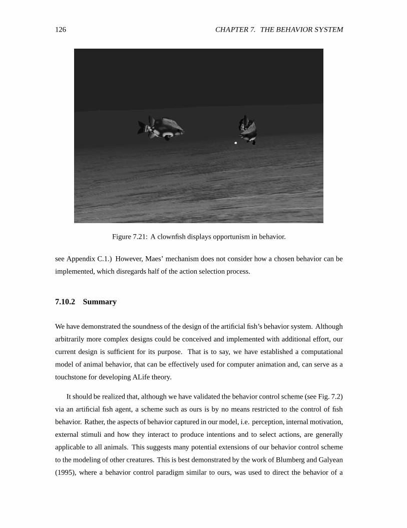
126 CHAPTER 7. THE BEHAVIOR SYSTEM
Figure 7.21: A clownfish displays opportunism in behavior.
see Appendix C.1.) However, Maes’ mechanism does not consider how a chosen behavior can be
implemented, which disregards half of the action selection process.
7.10.2 Summary
We have demonstrated the soundness of the design of the artificial fish’s behavior system. Although
arbitrarily more complex designs could be conceived and implemented with additional effort, our
current design is sufficient for its purpose. That is to say, we have established a computational
model of animal behavior, that can be effectively used for computer animation and, can serve as a
touchstone for developing ALife theory.
It should be realized that, although we have validated the behavior control scheme (see Fig. 7.2)
via an artificial fish agent, a scheme such as ours is by no means restricted to the control of fish
behavior. Rather, the aspects of behavior captured in our model, i.e. perception, internal motivation,
external stimuli and how they interact to produce intentions and to select actions, are generally
applicable to all animals. This suggests many potential extensions of our behavior control scheme
to the modeling of other creatures. This is best demonstrated by the work of Blumberg and Galyean
(1995), where a behavior control paradigm similar to ours, was used to direct the behavior of a
7.10. DISCUSSION 127
kinematic graphical dog creature.
On the one hand we realize that a crucial step in our behavior control scheme is the construction
of effective motor controllers. Realistic visual effects depend on how well the motor controllers can
control the underlying model of the animal, to produce realistic locomotion. On the other hand,
abstracting motor controllers is a necessary step towards the modeling of higher level behaviors.
Currently, motor control in complex creatures, such as articulated figures, remains an unsolved
problem. However when the underlying control problem for such creatures is solved, we believe
the design of our behavioral control scheme can provide the starting point for the modeling of the
behaviors of the animal in question. Thus, as we have stated in Chapter 2, the unavailability of
motor controllers for a particular animal, should not imply a lack of generality of the control scheme
we have proposed.
For animals that have complex cognitive abilities, additional control layers may be added on top
of the current control scheme. The current control scheme can serve as a reactive behavioral control
layer for the more basic behaviors of the animal, such as collision avoidance, foraging and mating.
Moreover, many higher animals possess actuators (e.g. limbs) that are beyond the necessity of
locomotion, for example, the arms and hands of primates and humans. These actuators may provide
a large number of motor skills relevant to manipulation which are mutually exclusive to those used
for locomotion. Consequently, the chances of being able to fulfill more than one intention at a time
are greatly increased. This suggests that it may be advantageous to permit multiple intentions to
be active simultaneously. For instance, a synthetic human actor should be able to fulfill both the
intention of searching for someone in a crowded room and the intention of not spilling a cup of
coffee.
Let us consider drawing a spectrum of various behavior control schemes, with the strictly
winner-takes-all and the free-flow selection processes occupying the two extremes. It is reasonable
to assume that a desirable control scheme would be a compromise between the extremes. In
particular, such a scheme should allow multiple intentions to be active simultaneously while still
maintaining reasonable simulation speed. This can be done by restricting the allowable number
of active intentions. In addition, in order to generate behavior-oriented, harmonic movements, a
more elaborate fusion mechanism at the motor level would be necessary to collect and combine the
resulting motor commands.

128 CHAPTER 7. THE BEHAVIOR SYSTEM
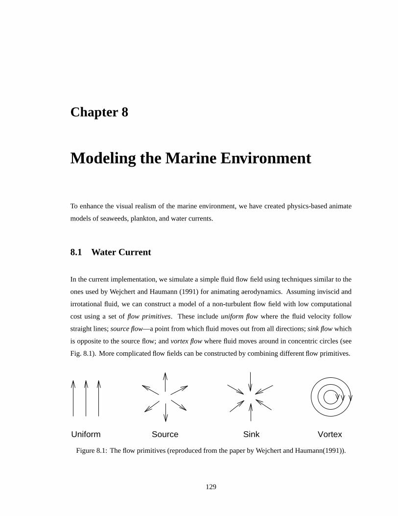
Chapter 8
Modeling the Marine Environment
To enhance the visual realism of the marine environment, we have created physics-based animate
models of seaweeds, plankton, and water currents.
8.1 Water Current
In the current implementation, we simulate a simple fluid flow field using techniques similar to the
ones used by Wejchert and Haumann (1991) for animating aerodynamics. Assuming inviscid and
irrotational fluid, we can construct a model of a non-turbulent flow field with low computational
cost using a set of flow primitives. These include uniform flow where the fluid velocity follow
straight lines; source flow—a point from which fluid moves out from all directions; sink flow which
is opposite to the source flow; and vortex flow where fluid moves around in concentric circles (see
Fig. 8.1). More complicated flow fields can be constructed by combining different flow primitives.
Uniform Sink VortexSource
Figure 8.1: The flow primitives (reproduced from the paper by Wejchert and Haumann(1991)).
129
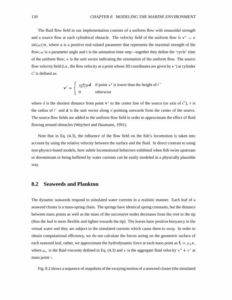
130 CHAPTER 8. MODELING THE MARINE ENVIRONMENT
The fluid flow field in our implementation consists of a uniform flow with sinusoidal strength
and a source flow at each cylindrical obstacle. The velocity field of the uniform flow is {�| �~}sin -^��� /C{ , where
}is a positive real-valued parameter that represents the maximal strength of the
flow; � is a parameter angle and � is the animation time step—together they define the ‘cycle’ time
of the uniform flow; { is the unit vector indicating the orientation of the uniform flow. The source
flow velocity field (i.e., the flow velocity at a point whose 3D coordinates are given by {�� ) at cylinder
b is defined as:
{ � �IK L ��!���@���!��� if point {�� is lower than the height of b� otherwise
where � is the shortest distance from point { � to the center line of the source (or axis of b ), � is
the radius of b and � is the unit vector along � pointing outwards from the center of the source.
The source flow fields are added to the uniform flow field in order to approximate the effect of fluid
flowing around obstacles (Wejchert and Haumann, 1991).
Note that in Eq. (4.3), the influence of the flow field on the fish’s locomotion is taken into
account by using the relative velocity between the surface and the fluid. In direct contrast to using
non-physics-based models, here subtle locomotional behaviors exhibited when fish swim upstream
or downstream or being buffeted by water currents can be easily modeled in a physically plausible
way.
8.2 Seaweeds and Plankton
The dynamic seaweeds respond to simulated water currents in a realistic manner. Each leaf of a
seaweed cluster is a mass-spring chain. The springs have identical spring constants, but the distance
between mass points as well as the mass of the successive nodes decreases from the root to the tip
(thus the leaf is more flexible and lighter towards the tip). The leaves have positive buoyancy in the
virtual water and they are subject to the simulated currents which cause them to sway. In order to
obtain computational efficiency, we do not calculate the forces acting on the geometric surface of
each seaweed leaf, rather, we approximate the hydrodynamic force at each mass point as uBv ���\� { ,
where�\�
is the fluid viscosity defined in Eq. (4.3) and { is the aggregate fluid velocity { | M { � at
mass point y .Fig. 8.2 shows a sequence of snapshots of the swaying motion of a seaweed cluster (the simulated
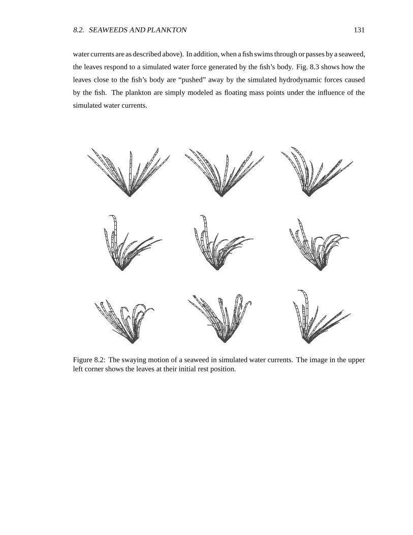
8.2. SEAWEEDS AND PLANKTON 131
water currents are as described above). In addition, when a fish swims through or passes by a seaweed,
the leaves respond to a simulated water force generated by the fish’s body. Fig. 8.3 shows how the
leaves close to the fish’s body are “pushed” away by the simulated hydrodynamic forces caused
by the fish. The plankton are simply modeled as floating mass points under the influence of the
simulated water currents.
Figure 8.2: The swaying motion of a seaweed in simulated water currents. The image in the upperleft corner shows the leaves at their initial rest position.
132 CHAPTER 8. MODELING THE MARINE ENVIRONMENT
Figure 8.3: The seaweed responds to hydrodynamic forces produced by a passing fish.
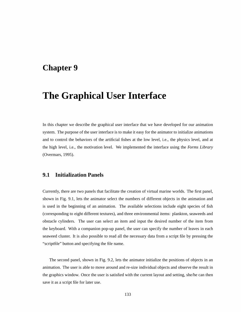
Chapter 9
The Graphical User Interface
In this chapter we describe the graphical user interface that we have developed for our animation
system. The purpose of the user interface is to make it easy for the animator to initialize animations
and to control the behaviors of the artificial fishes at the low level, i.e., the physics level, and at
the high level, i.e., the motivation level. We implemented the interface using the Forms Library
(Overmars, 1995).
9.1 Initialization Panels
Currently, there are two panels that facilitate the creation of virtual marine worlds. The first panel,
shown in Fig. 9.1, lets the animator select the numbers of different objects in the animation and
is used in the beginning of an animation. The available selections include eight species of fish
(corresponding to eight different textures), and three environmental items: plankton, seaweeds and
obstacle cylinders. The user can select an item and input the desired number of the item from
the keyboard. With a companion pop-up panel, the user can specify the number of leaves in each
seaweed cluster. It is also possible to read all the necessary data from a script file by pressing the
“scriptfile” button and specifying the file name.
The second panel, shown in Fig. 9.2, lets the animator initialize the positions of objects in an
animation. The user is able to move around and re-size individual objects and observe the result in
the graphics window. Once the user is satisfied with the current layout and setting, she/he can then
save it as a script file for later use.
133
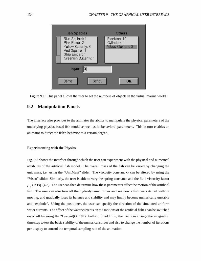
134 CHAPTER 9. THE GRAPHICAL USER INTERFACE
Figure 9.1: This panel allows the user to set the numbers of objects in the virtual marine world.
9.2 Manipulation Panels
The interface also provides to the animator the ability to manipulate the physical parameters of the
underlying physics-based fish model as well as its behavioral parameters. This in turn enables an
animator to direct the fish’s behavior to a certain degree.
Experimenting with the Physics
Fig. 9.3 shows the interface through which the user can experiment with the physical and numerical
attributes of the artificial fish model. The overall mass of the fish can be varied by changing the
unit mass, i.e. using the “UnitMass” slider. The viscosity constant � v can be altered by using the
“Visco” slider. Similarly, the user is able to vary the spring constants and the fluid viscosity factor�\�(in Eq. (4.3). The user can then determine how these parameters affect the motion of the artificial
fish. The user can also turn off the hydrodynamic forces and see how a fish beats its tail without
moving, and gradually loses its balance and stability and may finally become numerically unstable
and “explode”. Using the positioner, the user can specify the direction of the simulated uniform
water currents. The effect of the water currents on the motions of the artificial fishes can be switched
on or off by using the “Current(On/Off)” button. In addition, the user can change the integration
time step to test the basic stability of the numerical solver and also to change the number of iterations
per display to control the temporal sampling rate of the animation.
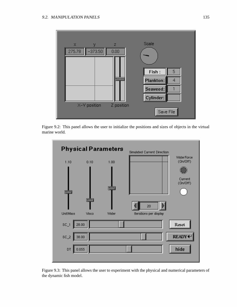
9.2. MANIPULATION PANELS 135
Figure 9.2: This panel allows the user to initialize the positions and sizes of objects in the virtualmarine world.
Figure 9.3: This panel allows the user to experiment with the physical and numerical parameters ofthe dynamic fish model.
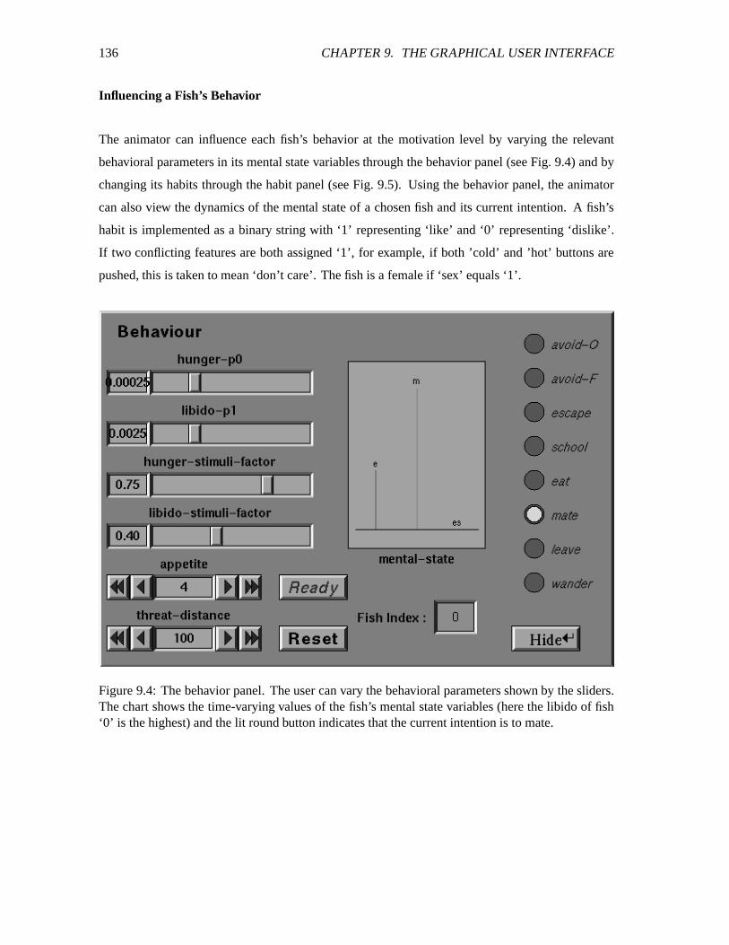
136 CHAPTER 9. THE GRAPHICAL USER INTERFACE
Influencing a Fish’s Behavior
The animator can influence each fish’s behavior at the motivation level by varying the relevant
behavioral parameters in its mental state variables through the behavior panel (see Fig. 9.4) and by
changing its habits through the habit panel (see Fig. 9.5). Using the behavior panel, the animator
can also view the dynamics of the mental state of a chosen fish and its current intention. A fish’s
habit is implemented as a binary string with ‘1’ representing ‘like’ and ‘0’ representing ‘dislike’.
If two conflicting features are both assigned ‘1’, for example, if both ’cold’ and ’hot’ buttons are
pushed, this is taken to mean ‘don’t care’. The fish is a female if ‘sex’ equals ‘1’.
Figure 9.4: The behavior panel. The user can vary the behavioral parameters shown by the sliders.The chart shows the time-varying values of the fish’s mental state variables (here the libido of fish‘0’ is the highest) and the lit round button indicates that the current intention is to mate.
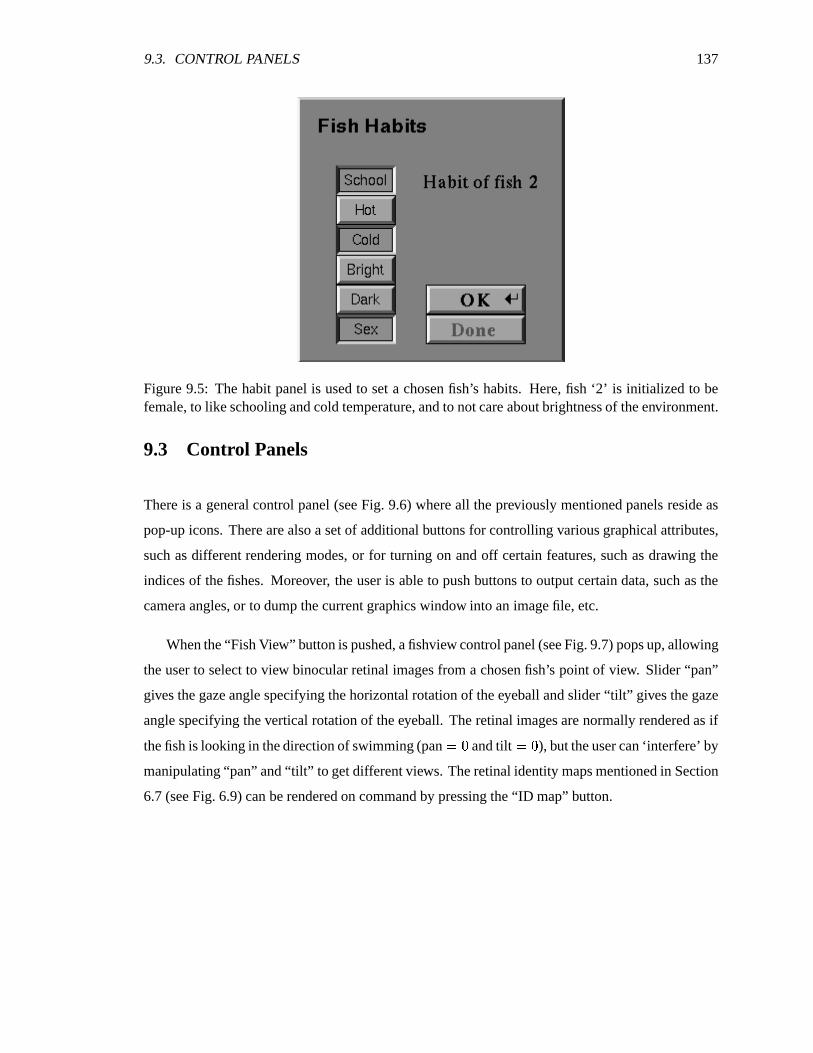
9.3. CONTROL PANELS 137
Figure 9.5: The habit panel is used to set a chosen fish’s habits. Here, fish ‘2’ is initialized to befemale, to like schooling and cold temperature, and to not care about brightness of the environment.
9.3 Control Panels
There is a general control panel (see Fig. 9.6) where all the previously mentioned panels reside as
pop-up icons. There are also a set of additional buttons for controlling various graphical attributes,
such as different rendering modes, or for turning on and off certain features, such as drawing the
indices of the fishes. Moreover, the user is able to push buttons to output certain data, such as the
camera angles, or to dump the current graphics window into an image file, etc.
When the “Fish View” button is pushed, a fishview control panel (see Fig. 9.7) pops up, allowing
the user to select to view binocular retinal images from a chosen fish’s point of view. Slider “pan”
gives the gaze angle specifying the horizontal rotation of the eyeball and slider “tilt” gives the gaze
angle specifying the vertical rotation of the eyeball. The retinal images are normally rendered as if
the fish is looking in the direction of swimming (pan ��� and tilt ��� ), but the user can ‘interfere’ by
manipulating “pan” and “tilt” to get different views. The retinal identity maps mentioned in Section
6.7 (see Fig. 6.9) can be rendered on command by pressing the “ID map” button.
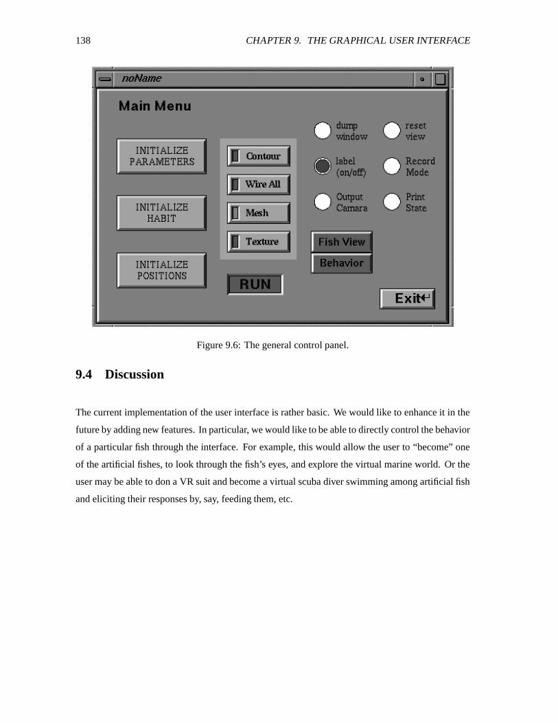
138 CHAPTER 9. THE GRAPHICAL USER INTERFACE
Figure 9.6: The general control panel.
9.4 Discussion
The current implementation of the user interface is rather basic. We would like to enhance it in the
future by adding new features. In particular, we would like to be able to directly control the behavior
of a particular fish through the interface. For example, this would allow the user to “become” one
of the artificial fishes, to look through the fish’s eyes, and explore the virtual marine world. Or the
user may be able to don a VR suit and become a virtual scuba diver swimming among artificial fish
and eliciting their responses by, say, feeding them, etc.
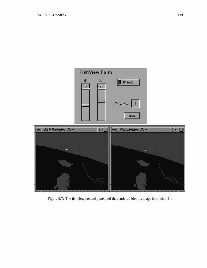
9.4. DISCUSSION 139
Figure 9.7: The fishview control panel and the rendered identity maps from fish ‘1’.

140 CHAPTER 9. THE GRAPHICAL USER INTERFACE
Chapter 10
Animation Results
The visual results of the research described in this dissertation are captured in a number of short
animation clips and two mini animation films “Go Fish!” and “A National Geo-Graphics Society
Special: The Undersea World of Jack Cousto”. “Go Fish!” was made in 1993 and was selected and
presented at the ACM SIGGRAPH’93 Electronic Theater Evening Program (Tu, Terzopoulos and
Fiume, 1993). “The Undersea World of Jack Cousto” was made in 1994 and was presented at the
ACM SIGGRAPH’95 Electronic Theater Evening Program. Both animations were subsequently
broadcast in various television science programs internationally. � “Go Fish!” has also won several
awards, including the 1994 Canadian Academy of Multimedia and Arts and Sciences International
Award for Technical Excellence. In the following sections, we briefly describe “Go Fish!” and “The
Undersea World of Jack Cousto”, as well as the contents of some additional animation shorts.
10.1 “Go Fish!”
“Go Fish!” runs for two minutes and four seconds and was produced by the author along with her
supervisors, Professor Demetri Terzopoulos and Professor Eugene Fiume.
The animation first illustrates the construction of a dynamic fish model. The mass-spring-damper
biomechanical substructure with its 12 primary contractile muscles is simulated in real time. The
substructure is then enclosed in a realistically shaped NURBS surface to create the fish body. The fish
�The interested reader is referred to the author’s home page http://www.dgp.toronto.edu/people/tu/go-fish.html for
a list of programs in which the two animations were shown.
141
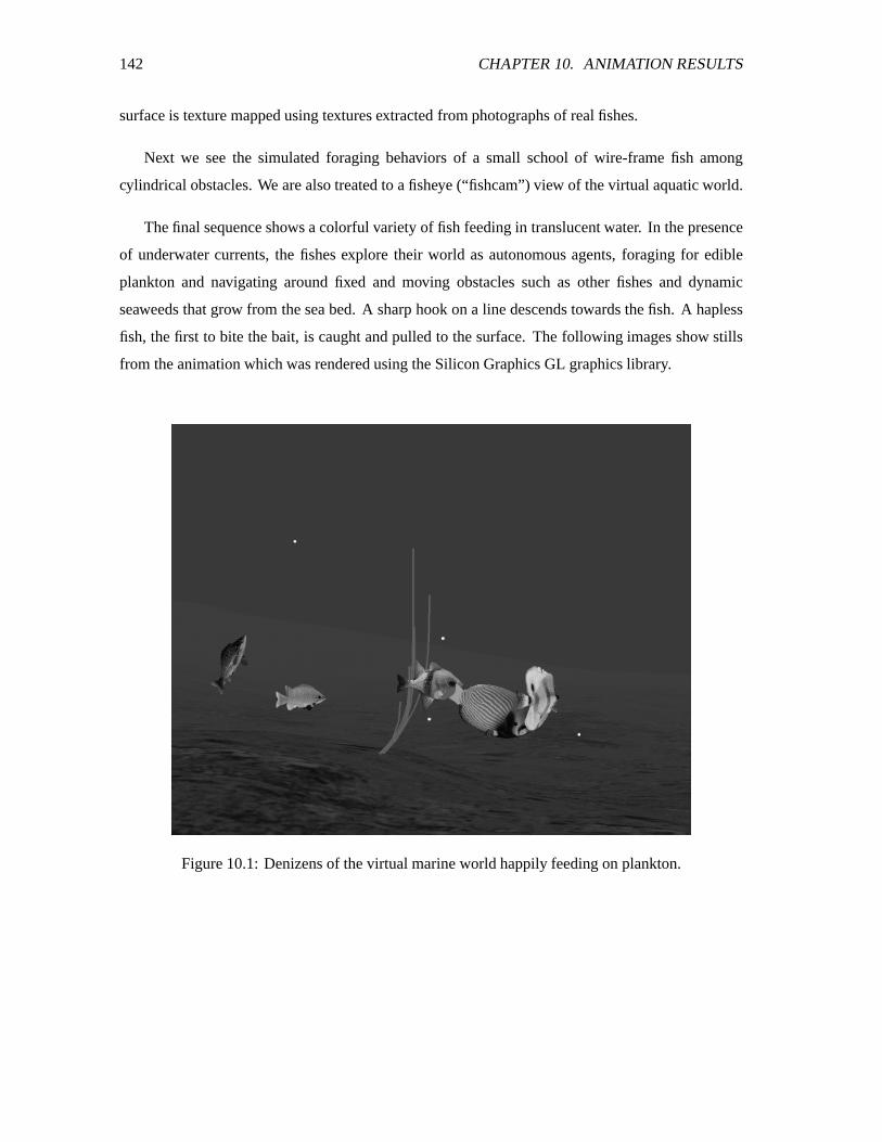
142 CHAPTER 10. ANIMATION RESULTS
surface is texture mapped using textures extracted from photographs of real fishes.
Next we see the simulated foraging behaviors of a small school of wire-frame fish among
cylindrical obstacles. We are also treated to a fisheye (“fishcam”) view of the virtual aquatic world.
The final sequence shows a colorful variety of fish feeding in translucent water. In the presence
of underwater currents, the fishes explore their world as autonomous agents, foraging for edible
plankton and navigating around fixed and moving obstacles such as other fishes and dynamic
seaweeds that grow from the sea bed. A sharp hook on a line descends towards the fish. A hapless
fish, the first to bite the bait, is caught and pulled to the surface. The following images show stills
from the animation which was rendered using the Silicon Graphics GL graphics library.
Figure 10.1: Denizens of the virtual marine world happily feeding on plankton.
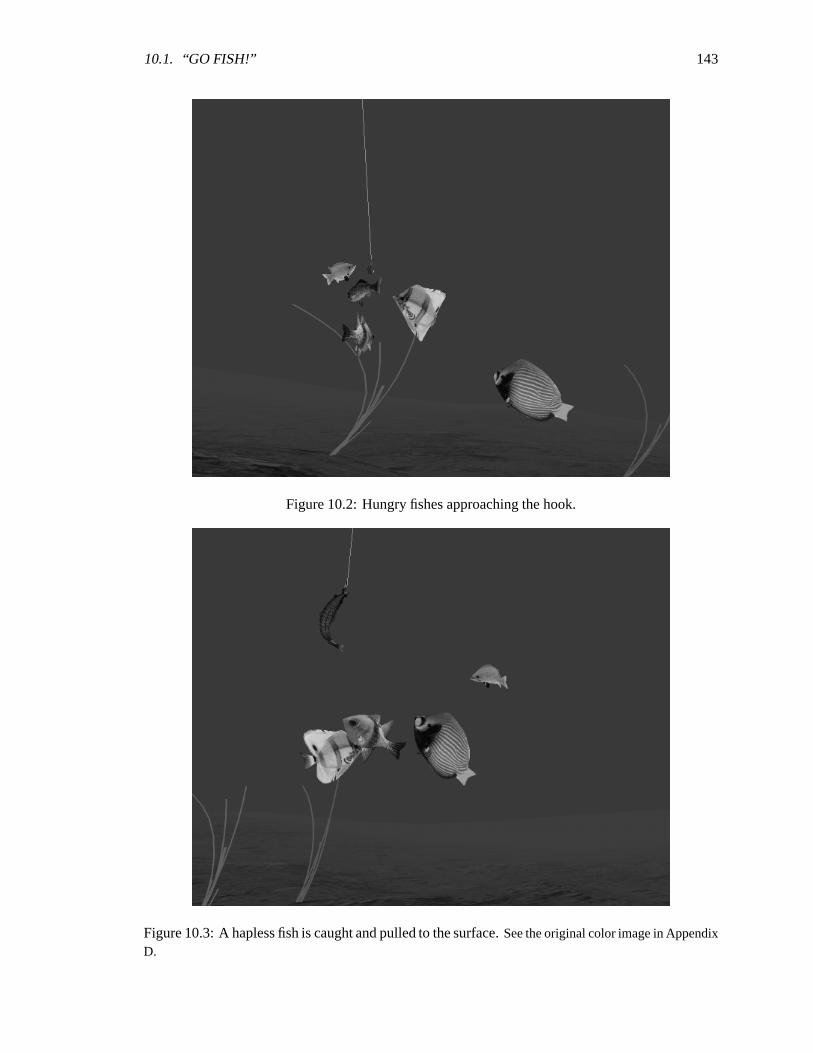
10.1. “GO FISH!” 143
Figure 10.2: Hungry fishes approaching the hook.
Figure 10.3: A hapless fish is caught and pulled to the surface. See the original color image in AppendixD.
144 CHAPTER 10. ANIMATION RESULTS
10.2 “The Undersea World of Jack Cousto”
The French oceanographer Jacques Cousteau has become legendary for his spectacular cinematog-
raphy of natural marine life. The reader may be familiar with the magnificent underwater doc-
umentaries produced by the Jacques Cousteau Foundation or those of the National Geographic
Society.
We have implemented an animation system that enables an animator to produce intriguing
“nature documentaries” of an artificial undersea world, not by conventional means, but by assuming
the role of a marine cinematographer analogous to that played by Cousteau. Unlike Cousteau,
however, who must deal with a physical camera in a physical world, our animator uses a virtual
camera to explore and record artificial life inhabiting a virtual marine world. To demonstrate this new
gender of computer animation, we have created a mini animated parody of a National Geographic
underwater documentary.
Our “National Geo-Graphics” documentary explores “The Undersea World of Jack Cousto”.
Jack’s cinematography reveals a mysterious world of colorful artificial fishes. We observe mating
rituals and other elaborate behaviors. Dangerous predators stalk in the deceptively peaceful habitat.
The following images show stills from the animation, which was rendered using the photorealistic
RenderManTM package.
“The Undersea World of Jack Cousto” runs for two minutes and thirty seconds and was produced
by the author along with her colleague Radek Grzeszczuk and Professor Demetri Terzoupoulos.
10.3 Animation Short: Preying Behavior
At the beginning of the animation, the ‘food chain’ phenomenon of a small underwater ecosystem is
displayed: various species of colorful ‘pacifist’ fishes are happily feeding on floating plankton (food
particles) while a ferocious predator fish is stalking a prey fish, hoping to devour it. The remainder
of the animation demonstrates the hunting behavior of the predator and the evasive behavior of the
prey. We see the greedy predator chasing after each prey until the prey is in close proximity, at
which point the predator opens its mouth and vigorously sucks in the prey. Moreover, we can see the
five reddish prey fish of the same species forming a school in an attempt to escape from the predator
while the predator is eating other prey. When the still hungry predator finally approaches the school,
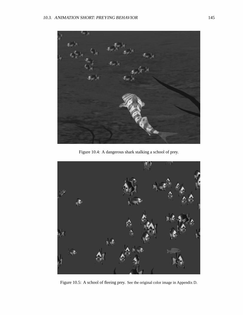
10.3. ANIMATION SHORT: PREYING BEHAVIOR 145
Figure 10.4: A dangerous shark stalking a school of prey.
Figure 10.5: A school of fleeing prey. See the original color image in Appendix D.
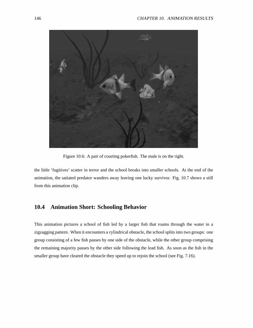
146 CHAPTER 10. ANIMATION RESULTS
Figure 10.6: A pair of courting pokerfish. The male is on the right.
the little ‘fugitives’ scatter in terror and the school breaks into smaller schools. At the end of the
animation, the satiated predator wanders away leaving one lucky survivor. Fig. 10.7 shows a still
from this animation clip.
10.4 Animation Short: Schooling Behavior
This animation pictures a school of fish led by a larger fish that roams through the water in a
zigzagging pattern. When it encounters a cylindrical obstacle, the school splits into two groups: one
group consisting of a few fish passes by one side of the obstacle, while the other group comprising
the remaining majority passes by the other side following the lead fish. As soon as the fish in the
smaller group have cleared the obstacle they speed up to rejoin the school (see Fig. 7.16).
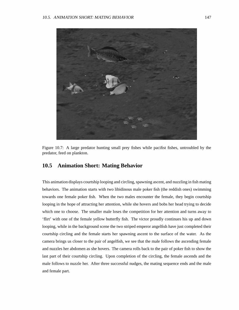
10.5. ANIMATION SHORT: MATING BEHAVIOR 147
Figure 10.7: A large predator hunting small prey fishes while pacifist fishes, untroubled by thepredator, feed on plankton.
10.5 Animation Short: Mating Behavior
This animation displays courtship looping and circling, spawning ascent, and nuzzling in fish mating
behaviors. The animation starts with two libidinous male poker fish (the reddish ones) swimming
towards one female poker fish. When the two males encounter the female, they begin courtship
looping in the hope of attracting her attention, while she hovers and bobs her head trying to decide
which one to choose. The smaller male loses the competition for her attention and turns away to
‘flirt’ with one of the female yellow butterfly fish. The victor proudly continues his up and down
looping, while in the background scene the two striped emperor angelfish have just completed their
courtship circling and the female starts her spawning ascent to the surface of the water. As the
camera brings us closer to the pair of angelfish, we see that the male follows the ascending female
and nuzzles her abdomen as she hovers. The camera rolls back to the pair of poker fish to show the
last part of their courtship circling. Upon completion of the circling, the female ascends and the
male follows to nuzzle her. After three successful nudges, the mating sequence ends and the male
and female part.

148 CHAPTER 10. ANIMATION RESULTS
Chapter 11
Conclusion and Future Work
11.1 Conclusion
In this dissertation we presented the results of research spanning the fields of computer graphics and
artificial life. With regard to computer graphics, we have proposed, implemented, and demonstrated
an animation framework that enables the creation of realistic animations of certain natural ecosystems
with minimal intervention from the animator. In our approach, the virtual creatures are self-
animating, as are real animals and humans. Thus, the strength of our approach to animation lies
in the fact that it turns the role of the animator from that of a graphical model puppeteer to that
of an virtual nature cinematographer, a job not unlike that done by nature cinematographers of
the National Geographic Society. Our artificial life approach has advanced the state-of-the-art of
computer animation, as evidenced by the unprecedented complexity and realism of the behavioral
animations that we have been able to achieve without keyframing. With regard to artificial life, we
have successfully modeled complete animals of nontrivial complexity. The convincing simulation
results validate our computational models, which capture the essential features of all biological
animals—biomechanics, locomotion, perception, and behavior.
In particular, we have developed a physics-based, virtual marine world inhabited by life-like
artificial life forms that emulate the appearance, motion, and behavior of fishes in their natural
habitats. Each artificial fish is an autonomous agent with a deformable body actuated by internal
muscles, with eyes, and with a brain that includes behavior, perception and motor centers. Through
controlled muscle actions, artificial fishes are able to swim through simulated water in accordance
with simplified hydrodynamics. Their functional fins enable them to locomote, maintain balance,
149
150 CHAPTER 11. CONCLUSION AND FUTURE WORK
and maneuver in the water. Though rudimentary compared to real animals, their brains are nonethe-
less able to capture many of the most important characteristics of animal behavior and carry out
perceptually guided motor tasks. In accordance with their perception of the virtual world and their
internal desires, their brains arbitrate a repertoire of behaviors and subsequently select appropriate
actions. The piscine behaviors the fishes exhibit include collision avoidance, foraging, preying,
fleeing, schooling, and mating. The easy extensibility of our approach to the modeling of additional
behaviors is suggested most evidently by the complex patterns of mating behavior that we have been
able to emulate in artificial fishes.
With regard to the implementation, we have pursued a bottom-up, compositional approach in
which we started by modeling the basic physics of the animal and its environment. Upon the
simulated physics substrate, we effectively modeled the animal’s means of locomotion. This in turn
positioned us to model the animal’s perceptual awareness of its world, its motivation, and last but
not least, its behavior. The compositional nature of our approach to synthesizing artificial fishes
was proven crucial to achieving realism. Partial solutions that do not adequately model physics,
locomotion, perception, motivation and behavior, and do not combine these models intimately within
the agent will not produce convincing results.
In addition to realism,computational efficiency has been one of the most important design criteria
of our implementation. The fidelity of our models was carefully chosen to achieve satisfactory com-
putational efficiency. We have strived successfully to achieve visually convincing animations with
low computational cost. Using a Silicon Graphics R4400 Indigo � Extreme workstation, a simulation
of ten artificial fishes, fifteen food particles and four static obstacles can run at about 4 frames/sec,
including wireframe rendering time and user interface running time. With a Reality Engine � graphics
board on the Silicon Graphics ONYX workstation, the same simulation with hardware-supported
GL, fully texture mapped surface rendering runs at about 3 frames/sec. Considering the complexity
of the animations, the simulation speed we have been able to achieve is more than satisfactory. The
main tradeoffs that we have made in order to gain high simulation speed is the simplification of the
virtual environment and the algorithms used for simulating the fish’s perceptual capability.
11.2 Additional Impact in Animation and Artificial Life
The work reported in this dissertation has promoted further research on automatic motion synthesis
for computer animation and on locomotion learning for artificial life. Grzeszczuk and Terzopoulos
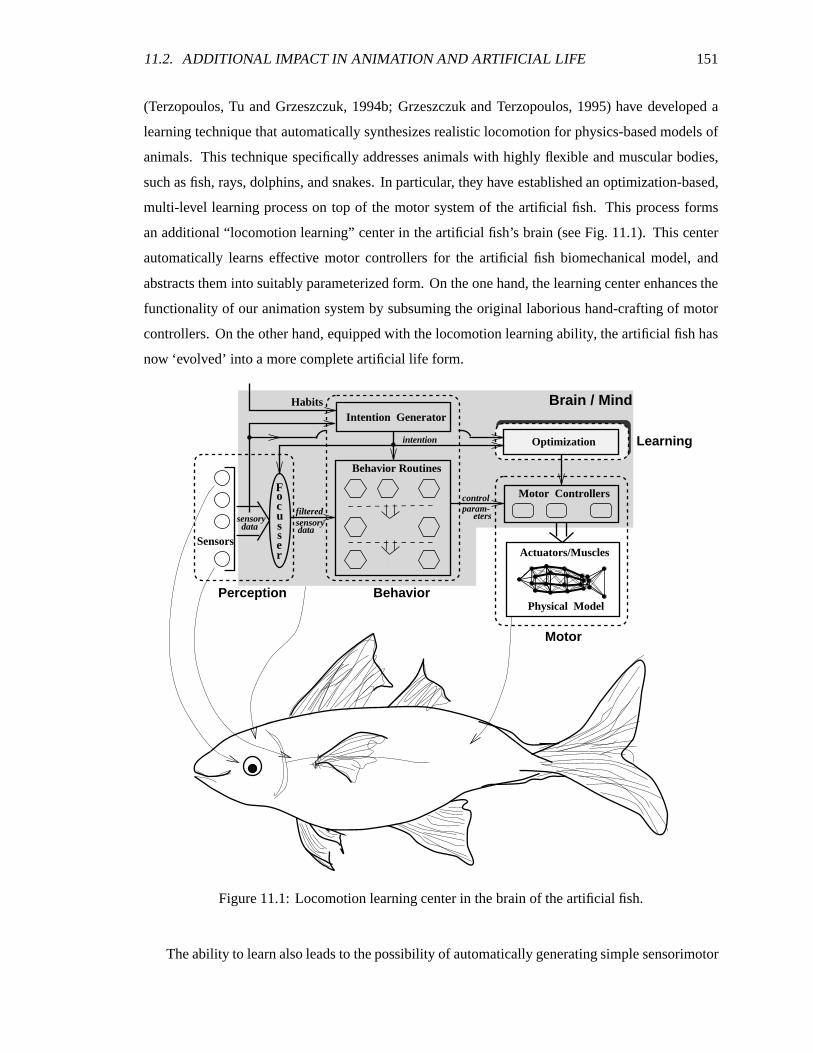
11.2. ADDITIONAL IMPACT IN ANIMATION AND ARTIFICIAL LIFE 151
(Terzopoulos, Tu and Grzeszczuk, 1994b; Grzeszczuk and Terzopoulos, 1995) have developed a
learning technique that automatically synthesizes realistic locomotion for physics-based models of
animals. This technique specifically addresses animals with highly flexible and muscular bodies,
such as fish, rays, dolphins, and snakes. In particular, they have established an optimization-based,
multi-level learning process on top of the motor system of the artificial fish. This process forms
an additional “locomotion learning” center in the artificial fish’s brain (see Fig. 11.1). This center
automatically learns effective motor controllers for the artificial fish biomechanical model, and
abstracts them into suitably parameterized form. On the one hand, the learning center enhances the
functionality of our animation system by subsuming the original laborious hand-crafting of motor
controllers. On the other hand, equipped with the locomotion learning ability, the artificial fish has
now ‘evolved’ into a more complete artificial life form.
filtered
Habits
control
Learning
Intention Generator
Actuators/Muscles
Motor Controllers
intention
Perception
Behavior Routines
Behavior
Brain / Mind
Sensors
sensory
param- eters
data
Physical Model
Optimization
sensorydata
Motor
coF
u
ress
Figure 11.1: Locomotion learning center in the brain of the artificial fish.
The ability to learn also leads to the possibility of automatically generating simple sensorimotor
152 CHAPTER 11. CONCLUSION AND FUTURE WORK
tasks for artificial animals, such as the fish. First steps along these lines have already been made:
Greszczuk and Terzopoulos (1995) imbue the artificial fish with the ability to learn to maneuver and
reach a visible target. This is done by enabling the animals to learn to put into practice the compact,
efficient controllers that they have previously learned. In this way, Grzeszczuk and Terzopoulos
have developed dolphin models that can learn to perform a variety of “SeaWorld stunts”.
11.3 Impact in Computer Vision and Robotics
Our work opens up several exciting avenues of research in related fields. For example, the software
that we have developed has made possible interesting new approaches to computer vision and
robotics.
Clearly the artificial fish is a situated virtual robot that offers a much broader range of perceptual
and animate capabilities, lower cost, and higher reliability than can be expected from present-day
physical robots like those described in (Maes, 1991b). For at least these reasons, artificial fishes
in their dynamic world can serve as a proving ground for theories that profess competence at
effectively linking perception to action (Ballard, 1991). To date, this thesis work has formed the
basis for computer vision research—an approach termed animat vision that has been pioneered by
Terzopoulos (Terzopoulos and Rabie, 1995; Terzopoulos, 1995).
The animat vision methodology employs artificial animals or animats as realistic, active observers
of their dynamic world. This approach can potentially liberate a significant segment of the computer
vision research community from their dependence on expensive robot hardware. It addresses the
needs of scientists who are motivated to understand and ultimately reverse engineer the powerful
vision systems found in higher animals. As is argued by Terzopoulos (1995),
Readily available hardware systems are terrible models of biological animals. For
lack of a better alternative, however, [vision scientists] have been struggling with
inappropriate hardware in their ambition to understand the complex sensorimotor
functions of real animals. Moreover, their mobile robots typically lack the compute
power necessary to achieve real-time response within a fully dynamic world while
permitting active vision research of much significance.
The artificial fishes and their habitats that we have developed are rich enough for grounding
biologically inspired active vision systems as is shown by Terzopoulos and Rabie (1995). They
11.4. POTENTIAL APPLICATIONS IN ETHOLOGY 153
have enabled active vision algorithms to be implemented entirely in software, thus circumventing
the problems of hardware vision.
11.4 Potential Applications in Ethology
A picture is worth a thousand words...
Ethologists have long hoped to simulate animals in computers in order to facilitate the systematic
study of animal behavior. As early as the seventies, ethologists Remy and Bernadette Chauvin
expressed their keen interest in such an approach to the analysis of animal behavior (Chauvin
and Muckensturm-Chauvin, 1977). More recently, McFarland (1993b) and Roiblat (1994) also
emphasized the importance of such an approach:
“It is possible that ethologists will profit to a greater extent from the possibilities offered
by simulation models... The availability of simulation programs makes it possible to
identify which instructions devolve from a purely ethological interpretation and which
from a cognitive one. A comparison of the program’s behavior with the behavior actually
displayed by the animal should enable the validity of the corresponding interpretation
to be assessed.” (Roiblat, 1994)
To this end, our artificial fish can act as a prototype model animal that provides a novel and potentially
useful investigative tool. Although in several ways crude at this stage, our model can be furnished
with more sophisticated behavioral mechanisms, more elaborate muscle models, etc.
Prior simulation models only allowed the modeling of one aspect of the problem to be investigated
in isolation. Our model of artificial animals exemplifies a unified and complete system that allows a
whole animal to be studied, from the biomechanical motor system to the perception-driven behavior
system within a physics-based virtual world. In this way our approach allows the investigation of
complex interactions between these different levels.
Moreover, the results of our simulation are displayed in a convenient and easy to interpret form.
In effect what we have produced can be viewed as a sophisticated scientific visualization tool for
ethologists that may enable new insights to be gleaned and new relationships discovered. Our work
demonstrates the potential of realistic computer animation in applications to ethology.
154 CHAPTER 11. CONCLUSION AND FUTURE WORK
11.5 Other Artificial Animals
The title of this dissertation emphasizes the generality of our artificial animal approach to computer
animation, rather than its specific application in this thesis to fishes. The main components of our
approach—modeling form and appearance, biomechanics, locomotion, perception, and behavior—
carry over to the realistic modeling of other animals, although the details of each of these components
may, to one degree or another, be animal specific. Consider, for example, the design of a realistic
artificial cat.
� It is important to capture natural feline form and appearance, but clearly cats and fish differ
dramatically, so different 3D models and textures would be needed to model a cat.
� Cat biomechanics obey Newton’s laws of motion, as do fish biomechanics. Quite unlike
the highly deformable fish body, however, an artificial cat would require the biomechanical
modeling of an articulated skeleton actuated by skeletal muscles.
� With regard to locomotion, there are obvious differences between the hydrodynamic swimming
of a fish and the natural quadrupedal gait of the cat that exploits gravity and friction due to
foot-ground contact. Nevertheless, for both the fish and the cat, it is crucial to the design of
the higher level behavioral modeling to abstract the locomotion ability of the animal into a set
of parameterized motor controllers.
� Perceptual modeling is essential in both the cat and the fish. The perception model that we
have developed can with slight modification emulate the basic visual capabilities of a cat, but
one may also wish to model the auditory capability of cats.
� The artificial cat requires a behavior system at least as sophisticated at the one for the artificial
fish, including habits, mental state, an intention generator and behavior routines. Certain
innate characteristics, such as gender, mental variables, such as hunger, and behaviors, such
as collision avoidance, are common to both fish and cats, but behaviors such as scratching
in the litterbox are feline specific and would require the implementation of specific behavior
routines. However, the structure of our behavior control scheme remains appropriate.
To develop more complex artificial animals patterned after humans and other primates that have
sophisticated intelligent behaviors,our approach can serve in the development of a reactive behavioral
substrate that supports a higher-level reasoning system.
11.6. FUTURE RESEARCH DIRECTIONS 155
11.6 Future Research Directions
11.6.1 Animation
The behavioral animation system that we have proposed and demonstrated can be improved and
further developed in many aspects. We are interested in exploring future research in a number of
directions.
Physics-based Motor Control
Physics-based modeling offers many advantages and has, in our case, proven to be successful in
generating realistic motions of fishes. However, the associated control problem for more complicated
creatures remains a difficult endeavor. We would like to explore ways of simplifying the control
problem, perhaps by exploiting analytical solutions to the given physical system.
Better Hydrodynamics and a Greater Variety of Marine Animals
In the current implementation of the artificial fish system, we model only simplified hydrodynamics
in the virtual environment. An interesting future research direction would be to establish more
sophisticated models of hydrodynamics. This would allow us to further examine the complex
interactions between the characteristics of such a hydrodynamic environment and the motion and
behavior of the artificial fishes. Furthermore, we want to implement more marine animals to enhance
our virtual undersea world, such as eels, seahorses and jellyfish, etc.
More Elaborate Perception Model
As we have mentioned in Chapter 6, we would like to develop more sophisticated algorithms for
modeling artificial animal’s perception in more complex virtual environment. We are also interested
in synthesizing various elaborate sensing abilities of animals, for instance, modeling diffusion for
olfactory sensing.
156 CHAPTER 11. CONCLUSION AND FUTURE WORK
Modeling Emotion for Behavior Control
Emotion is an important factor of animal behavior. It plays an essential role in describing the
‘personalities’ of an animal. Unlike habits, the emotion of an animal is typically associated with one
or more specific objects, rather than with some generic condition. The involvement of emotion may
often cause an animal to exhibit ‘unusual’ behavior. For example, although is generally friendly to
humans, a cat may dislike a particular person and react strongly against him/her. We would like to
incorporate a model of emotion into our behavior control scheme to enhance the behavior realism
of the animals being animated. This model will allow additional differentiation between characters
in an animation as well as offering additional high-level means of controlling their behavior.
Higher Directability
Last but not least, we would like to explore an intuitive way of directing the autonomous artificial
creatures to a high degree. In the current implementation, it is easiest to create animations in which
we do not demand highly specific control over what the creatures do and when they do it, as long
as they behave naturally. However, it is not unusual to want to create an animation which shows,
say, two or more events happening at roughly the same time and place. For example, when making
the animation “The Undersea World of Jack Cousto” (Tu, Grzeszczuk and Terzopoulos, 1995), we
wanted to show, in a period of less than one minute of animation, two fishes displaying mating
rituals while a large school of fish passes by in the background stalked by a predator shark. The most
difficult part of achieving this sort of scenario is to roughly synchronize the mating, the schooling
and the preying and to make schooling/preying happen in roughly the right place (the background). �To achieve these sorts of synchronizations, the animator would have to spend a fair amount of
time performing multiple trials, tuning the relevant parameters until the desired action sequence is
achieved. An obvious way of simplifying the problem is to suspend the forward simulation of the
school of fish and the shark and run a trial simulation to determine the time at which the mating
occurs. Once this is known, we can start simulating the school of fish and the shark roughly around
the same time. Of course, we may still need to influence the path of the school which is done by
scripting the path of the ‘lead’ fish. Currently, these detailed manipulations are done by hand and
hence may be cumbersome.
�It is easy to let the mating happen early into the animation by setting the libido parameter of the two fishes high
enough.
11.6. FUTURE RESEARCH DIRECTIONS 157
It may be possible, however, to build a higher level controller on top of the animation system we
currently have in order to accomplish similar tasks in a much more convenient way. A promising
approach for accomplishing this level of control would be employ some descriptive language for
monitoring the animation process and exerting direct control over the various aspects of the simula-
tion; e.g. the start time of some specific creatures and their paths, etc. Therefore, one of the future
research directions could be to define and develop such a language and its interface to the current
animation system. Blumberg and Galyean (1995) recently proposed and implemented a system that
addresses interactive “directability” of animated autonomous creatures. Their work marked a first
step towards the aforementioned future research direction.
11.6.2 Artificial Life
The long-term goal of our research in the regard of artificial life is a computational theory that can,
potentially, account for the interplay of locomotion, perception and behavior in higher animals. We
believe that a good touchstone of such a theory is its ability to produce visually convincing results
in the form of realistic computer graphics animations with little or no animator intervention. �An obvious research direction would address the goals of researchers interested in evolving
artificial life. We may be within reach of computational models that can imitate the spawning
behaviors of the female fish and fertilization by the male. Through simulated sexual reproduction
in a competitive world, gametes representing artificial fish genotypes can be fused to evolve new
varieties of artificial fishes. Interestingly, Pokhilko, Pajitnov, et al., have already demonstrated the
simulated breeding of fish models much simpler than ours using genetic algorithms, and this idea
has resulted in the fascinating computer game program “El-Fish” (Corcoran, 1992).
�In the context of artificial life there are no constraints on what should happen when.
Appendix A
Deformable Contour Models
A “snake” (Kass, Witkin and Terzopoulos, 1987) is a dynamic deformable contour in the x-y image
plane. We define a discrete deformable contour as equally-spaced nodes indexed by ���� ������� ,
with time varying positions ��������� ����� ������� � ���!�"��# . The deformable contour’s dynamic behavior
can be influenced interactively by incorporating user-specified forces (e.g. mouse forces) into its
equations of motion. Such behavior is governed by the system of first-order ordinary differential
equations:$&% �'�
% �(*) � (*+ � �-, �/. �0�� 1�2���� (A.1)
where $ is a velocity-dependent damping constant,) � ����� are “tension” forces which make the
deformable contour act like a series of springs that resist deformation,+ �����"� are “rigidity” forces
which make the contour act like thin wire that resists bending, and , �!����� are forces in the image plane,13� ����� plus the simulated mouse forces applied to the contour.
A 4657 deformable mesh consists of 4 ( contours, of which run vertically, each with 4nodes, and 4 of which run horizontally each with nodes. The crossing points on the deformable
mesh are nodes shared by the intersecting contours.
We express) � , the tension forces, in terms of the deformation of the springs connecting node
to its two neighboring nodes and+ � , the rigidity forces, in terms of the second order forward finite
differences as follows: ) � ��8 ��9:��;1�=< 8 �?> � 9:�?> � ;��@> � (A.2)
+ � ��A ��B � �!����B � <DCE����B � ( ������<FC A ��������B � <FCE��� ( �'�@> � � ( A �?> � �����G<FCE���?> � ( �'�@> � � (A.3)
158
159
where 8 and A are parameters, 9 � is the deformation of the spring connecting node to node ( �(i.e. its current length minus its rest length), and ;�� is the unit vector from ��� to ����B � . Note that
) �and
+ � vanish in the absence of deformation and bending.
To make the outline of the fish in the image stand out, we convert the original RGB color image
into a gray-scale image H=� �' � � . The gradient of H , call it I 3 � �� J� � , forms a potential field whose
“ravines” coincide with the dark outline of the profile of the fish. The image force field can then be
expressed as the gradient of I 3 � �� J� � , i.e. , 3� ��K I 3 � �' � � ) such that the ravines act as attractors
to deformable contours. The contours descend and stabilize at the bottoms of the nearest ravines.
In order to let the ravines attract the deformable contours from some distance away, the potential
function I 3 � �� � � is computed as follows:
I 3 � �� � � ��LNMPORQ�QSK HG� �� � � QTQT
where L M O denotes convolution with a 2D Gaussian smoothing filter of width U which broadens the
ravines of K H .
Often the user may initialize the border of the deformable mesh too far from the edges of the
fish body and hence the deformable contours may become attracted by nearby dark features and fail
to localize the correct outline. Should this be the case, the user can apply simulated spring forces,1V� ���"� by using the mouse to guide a deformable contour towards the ravine of interest (Kass, Witkin
and Terzopoulos, 1987).
Another case frequently encountered is where the profile of the fish is not composed of edges
that are consistently dark or consistently white. For example, in the fish image shown in Fig. 5.6(a),
part of the profile that bounds the tail and the upper body is made of white edges while the lower
body is demarcated from the background by dark lines. In this case if , 3� is generated such that the
deformable contours are attracted to dark edges then most of the profile in Fig. 5.6(a) can not be
captured properly. It is hence useful to constrain certain nodes of the border contours to selected
anchor points WE� in the image (the interface allows the user to interactively place anchor points using
the mouse). The constraints prevent the deformable contours from straying far from the anchor
points, regardless of the image forces and other mouse forces. This can be achieved by attaching
the deformable contour nodes with springs to their corresponding anchor points:
,EX� �ZY �[W\�]<^���_�

160 APPENDIX A. DEFORMABLE CONTOUR MODELS
where Y is the spring constant. Using this mechanism we can also effectively deal with images
where the profile of the fish is obscure.
The total external force , � is therefore obtained by combining the image force , 3� , the mouse
force , V� and the constraint force , X� . The deformable contour can then be simulated by integrating
the system of ordinary differential equations (A.1) forward through time using an Euler integration
method (Press et al., 1986).
Appendix B
Visualization of the Pectoral Motions
The geometric model of a pectoral fin is a five-vertex polygonal surface with one vertex, i.e. the
“root”, fixed at a certain control point of the NURBS surface of the display fish model. Let us denote
the root vertex as `ba and the four other vertices, ordered clockwise, as ` � to `�c respectively (see
Fig. B.1(a)). The visualization problem is then to determine the time-varying trajectories of `�� , �d�� C ef �g . It is reasonable to assume constant lengths of the vectors `ba�� , �d�� C Jef "g pointing
from ` a to the other vertices. Therefore the control problem becomes that of determining the
directions of these vectors over time.
Expressing vectors ` a�� , �h�� C ef /g , in the fish’s local coordinate system (see Fig. 4.14)
simplifies the implementation of the fin motions. Once the new positions of `ia!� ’s are computed in
the fish’s local coordinate system, they are transformed back to the world coordinates system for
graphics display.
B.1 Animating the Pectoral Flapping Motion
To achieve the flapping motion, let us define displacement vectors jk�!���"� which, when added to `ba�� , �l�� C em /g , yield the new directions of ` a�� . Let the normal of the plane formed by ` a � and ` a!cbe a unit vector `'n . The pectoral flapping motions are modeled by simply specifying the direction
of the displacement vectors jo�!���"� along `�n and then letting the lengths of jo�!����� vary over time in a
161
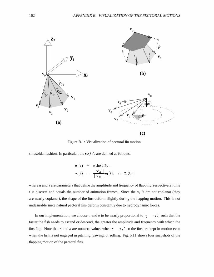
162 APPENDIX B. VISUALIZATION OF THE PECTORAL MOTIONS
θ
v r
(a)
x
y
z
f
f
f
v01
vvv04 03
02
0v
v1
(c)
e
0v
3v
(b)
0v
v1
v4
2v
3v
v1
2vv
4
Figure B.1: Visualization of pectoral fin motion.
sinusoidal fashion. In particular, the j � �!�"� ’s are defined as follows:
j � ����� � 8qp!r@s � A �"�!`�n j � ����� � t ` a!� t
t `ia � t j � �!�"� � C em "gG
where 8 and A are parameters that define the amplitude and frequency of flapping, respectively; time
� is discrete and equals the number of animation frames. Since the `ia!� ’s are not coplanar (they
are nearly coplanar), the shape of the fins deform slightly during the flapping motion. This is not
undesirable since natural pectoral fins deform constantly due to hydrodynamic forces.
In our implementation, we choose 8 and A to be nearly proportional to Q $ <FubvwC Q such that the
faster the fish needs to ascend or descend, the greater the amplitude and frequency with which the
fins flap. Note that 8 and A are nonzero values when $ � uxvwC so the fins are kept in motion even
when the fish is not engaged in pitching, yawing, or rolling. Fig. 5.11 shows four snapshots of the
flapping motion of the pectoral fins.
B.2. ANIMATING THE PECTORAL OARING MOTION 163
B.2 Animating the Pectoral Oaring Motion
The oaring motion of the pectoral fins is most distinguishable in natural fishes with relatively large,
flat bodies that do not bend as much when swimming or turning. We capture this visual detail in our
artificial butterfly fish and emperor angelfish.
To achieve the oaring motion of the pectoral fins, we let `'� , �y�z C Jef "g rotate about a pre-
defined unit vector `�{ such that each `ia!� traces out a cone shape (see Fig. B.1(c)). The rotation
is computed using unit quaternions | � �[}J~ p �/��vECk� �p!r@s �/��vECk��`�{:� , where � is the rotation angle
(Shoemake, 1985). Let the initial `ba�� , before rotation, be denoted by `x�a!� , then we can compute the
new `ba�� with the formula
� �f ` a!� � ���|z� �f ` �a!� �/|where �| denotes the conjugate of | . With � varying from 0 to C�u , each `ia!� sweeps a complete cone
corresponding to one full stroke of rowing. The speed with which � changes represents the speed
of rowing. We choose � � + � where parameter+
is proportional to the fish’s swimming speed Q2Q ` Q2Qthus the faster the fish swims the faster the fins beat. Note that the above | defines a “forward”
oaring motion towards the direction of swimming ��� . To obtain a backward oaring motion, we can
simply let | � �[}J~ p �[�zvwC�� < p!r@s �[�zvwC���`�{J� .In our animations, when a butterfly fish or an emperor angelfish turns, one of the pectoral fins
rows forward and the other backward as is observed in many natural, flat-body fishes. The backward
oaring motions of both fins are useful when an artificial fish brakes and retreats. Fig. 5.12 shows
snapshots of a butterfly fish with its forward oaring pectoral fins.
Appendix C
Prior Action Selection Mechanisms
C.1 Behavior Choice Network
Maes (1990; 1991a) proposed a distributed, non-hierarchical mechanism which takes into account
both internal and external stimuli in making behavioral choices. The nodes of the network represent
behavior units and are connected by special purpose links, such as inhibitory links. The overall
behavior of the network is an emergent property of interactions among the nodes, and of interactions
between the nodes and the environment. More specifically, activation energy flows from both
external sensory readings and internal motivations to different behavioral components. Different
components use the links of the network to excite and inhibit each other. After some time, the
activation energy accumulates in the component that represents the “best” choice, which is taken
as the winner, given the current situation and motivational state of an agent. This mechanism was
originally used, and proven successful, in solving relatively simple problems in a traditional AI
setting (i.e. blocks world), such as choosing actions in a correct sequence so as to sand a board or
spray paint a block (Maes, 1990). By incorporating some biological aspects into the mechanism, it
is able to deal with more complex action selection problems (Maes, 1991a).
The main advantages of Maes’ action selection mechanism are: first, the activation energy is
a continuous flow which allows smooth transition from behavior to behavior; second, it is more
flexible and reactive as opposed to being centrally controlled; finally, the distributed structure makes
the action selection process more robust.
Some limitations have also been pointed out by Maes herself and others (Sahota,1994; Blumberg,
164
C.2. FREE-FLOW HIERARCHY 165
1994). For example, it is not clear how to achieve global functionality using this mechanism and
careful tuning of parameters is needed. However, this is common to practically all distributed
architectures and is not unique to this work. Also, since sensory inputs of each node are in the form
of binary predicates, potentially useful information may be discarded. Moreover, Tyrrell (1993a) has
made a critical investigation of the strictly non-hierarchical and distributed computational structure
used by Maes. It is believed that the underlying structure for action selection, as suggested by
ethologists, is intrinsically hierarchical, rather than “flatly” distributed. It is argued that some of the
computational deficiencies due to the non-hierarchical structure of Maes’ mechanism indicate that
it is not well able to deal with animal-like action selection problems (Tyrrell, 1993a).
C.2 Free-Flow Hierarchy
In order to allow the combining of evidence from different behavioral candidates and the selection
of compromised actions, roboticists Rosenblatt and Payton (Rosenblatt and Payton, 1989) proposed
an alternative action selection process. In their mechanism, all behavior nodes express preferences
for each of a set of motor actions, rather than making a decision as to which is the most suitable.
The final choice is a weighted sum of all the preferences. This method was later extended by
Tyrrell (1993b) to form what is known as free-flow hierarchies. A free-flow hierarchy implements
Rosenblatt and Payton’s selection process within a hierarchical action selection architecture like
that of Tinbergen (1951). All nodes in the hierarchy can influence the subsequent behavior of the
agent. Activities express weighted preferences for activities lower in the hierarchy. This process
propagates throughout the whole hierarchy, and as a result, instead of making a decision at each
layer, a decision is only made at the lowest (i.e. action) level when the most highly preferred motor
action is chosen.
Simulation results (Tyrrell, 1993a) show that the free-flow hierarchy outperforms Maes’ mech-
anism and several other mechanisms. However, as Blumberg (1994) points out, the relatively better
performance of free-flow hierarchies may be gained at the expense of high complexity and low effi-
ciency. This is because no focus of attention is employed in a free-flow hierarchy, and preferences
need to be carefully weighted. In particular, real-time solutions may not be possible since decisions
can only be made after all sensory information is processed and preferences from all components are
calculated. Furthermore, all hierarchical structures suffer from a lack of flexibility in the sense that
connections between components, i.e. precedences, cannot be easily altered. Free-flow hierarchies
are no exception.
166 REFERENCES
References
Adler, H. E. (1975). Fish Behavior: Why Fishes do What They Do. T.F.H Publications, NeptuneCity, NJ.
Agre, P. and Chapman, D. (1987). Pengi: An implementation of a theory of activity. Proc. of AAAI,pages 268–272.
Alexander, R. (1982). Locomotion of Animals. Chapman & Hall, New York.
Alexander, R. (1983). Animal Mechanics. Blackwell Scientific Publications, Oxford, England, 2ededition.
Alexander, R. (1992). Exploring Biomechanics. Scientific American Library, New York.
Anderson, T. and Donath, M. (1990). Animal behavior as a paradigm for developing robot autonomy.In Robotics and Autonomous Systems, number 6, pages 145–168. Elservier Science PublishersB.V., North-Holland.
Armstrong, W. and Green, M. (1985). The dynamics of articulated rigid bodies for purposes ofanimation. The Visual Computer, 1(4):231–240.
Badler, N., Barsky, B., and Zeltzer, D. (1991). Making Them Move. Morgan Kaufmann.
Badler, N., Phillips, C., and Webber, B. (1993). Simulating Humans: Computer Graphics Animationand Control. Oxford University Press, New York.
Ballard, D. (1991). Animate vision. Artificial Intelligence, (48):57–86.
Barrow, H. G. and Tenenbaum, J. M. (1981). Computational vision. Proceedings of the IEEE,69(5):572–595.
Barzel, R. and Barr, A. H. (1988). A modeling system based on dynamic constraints. ACM ComputerGraphics, SIGGRAPH’88, 22(4):179–188.
Bathe, K.-J. and Wilson, E. L. (1976). Numerical Methods in Finite Element Analysis. Prentice-Hall,Englewood Cliffs, New Jersey.
Beer, R. (1990). Intelligence as Adaptive Behavior. Academic press, NY.
Beer, R. and Chiel, H. (1991). The neural basis of behavioral choice in an artificial insect. In Meyer,J.-A. and Wilson, S., editors, From Animals to Animats: The First International Conference onSimulation of Adaptive Behavior, pages 247–254. The MIT Press, Cambridge, MA.
Blake, R. (1983). Fish Locomotion. Cambridge University Press, Cambridge, England.
Blumberg, B. (1994). Action-selection in hamsterdam: Lessons from ethology. In Cliff, D., Hus-bands, P., Meyer, J.-A., and S, W., editors, From Animals to Animats: The Third InternationalConference on Simulation of Adaptive Behavior, pages 108–117. The MIT Press, Cambridge,MA.
Blumberg, B. and Galyean, T. (1995). Multi-level direction of autonomous creatures for real-timevirtual environments. In ACM Computer Graphics, Annual Conference Series, Proceedings ofSIGGRAPH’95, pages 47–54, Los Angeles, CA. ACM Computer Graphics.
REFERENCES 167
Braitenberg, V. (1984). Vehicles, experiments in synthetic psychology. The MIT Press, Cambridge,Massachusetts.
Brooks, R. (1986). A robust layered control system for a mobile robot. IEEE Journal of Roboticsand Automation, 1(RA-2):14–23.
Brooks, R. (1991). Intelligence without representation. Artificial Intelligence, (47):139–159.
Calvert, T. W., Chapman, J., and Patla, A. (1980). The integration of subjective and objective datain the animation of human movement. In Computer Graphics (SIGGRAPH ’80 Proceedings),volume 14, pages 198–203.
Carlbom, I., Terzopoulos, D., and Harris, K. M. (1994). Computer-assisted registration, segmen-tation, and 3D reconstruction from images of neuronal tissue sections. IEEE Transactions onmedical imaging, 13(2):351–362.
Chauvin, R. and Muckensturm-Chauvin, B. (1977). Behavioral Complexity. International Univer-sity Press, New York.
Cliff, D., Husbands, P., Meyer, J.-A., and S, W., editors (1994). From Animals to Animats: TheThird International Conference on Simulation of Adaptive Behavior, Cambridge, MA. TheMIT Press.
Coderre, B. (1987). Modeling behavior in Petworld. Artificial Life: The proceedings of an interdis-ciplinary workshop on the synthesis and simulation of living systems, VI:407–420.
Corcoran, E. (1992). One fish, two fish: How to raise a school of tempting software toys. ScientificAmerican.
Dawkins, R. (1976). Hierarchical organization: A candidate principle for ethology. In Bateson, P.and R., H., editors, Growing Points in Ethology. Cambridge University Press.
Dawkins, R. (1989). The Selfish Gene. Oxford University Press, Oxford, England, 2ed edition.
Foley, J., van Dam, A., Feiner, S., and Hughes, J. (1990). Computer Graphics Principles andPractice. Addison-Wesley, 2 edition.
Funge, J. (1995). Constraints and computer animation. Ph.D. Qualifying Exam Paper.
Girard, M. (1991). Constrained optimization of articulated animal movement in computer animation.In Badler, N., Barsky, B., and Zeltzer, D., editors, Making Them Move. Morgan Kaufmann.
Grzeszczuk, R. and Terzopoulos, D. (1995). Automated learning of muscle-actuated locomotionthrough control abstraction. ACM Computer Graphics, SIGGRAPH’95 Annual ConferenceProceedings, pages 63–70.
Hodgins, J., Wooten, W., Brogan, D., and O’Brien, J. (1995). Animating human athletics. In ACMComputer Graphics, Annual Conference Series, Proceedings of SIGGRAPH’95, pages 71–78,Los Angeles, CA. ACM Computer Graphics.
Hodgins, J. K., Sweeney, P. K., and Lawrence, D. G. (1992). Generating natural-looking motion forcomputer animation. Graphics Interface, pages 265–272.
168 REFERENCES
Isaacs, P. and Cohen, M. (1987). Controlling dynamic simulation with kinematic constraints, behav-ior functions, and inverse dynamics. ACM Computer Graphics, SIGGRAPH’87, 22(4):215–224.
Kaelbling, L. (1987). An architecture for intelligent reactive systems. In Proceedings of the 1986Workshop: Reasoning about Actions and Plans. Morgan Kaufmann.
Kass, M., Witkin, A., and Terzopoulos, D. (1987). Snakes: Active contour models. InternationalJournal of Computer Vision, 1(4):321–331.
Langton, C. G., editor (1987). Artificial Life: The proceedings of an interdisciplinary workshop onthe synthesis and simulation of living systems, volume VI. Aanta Fe Institute, Studies in theSciences of Complexity, Addison-Wesley.
Lasseter, J. (1987). Principles of traditional animation applied to 3D computer animation. In Stone,M. C., editor, Computer Graphics (SIGGRAPH ’87 Proceedings), volume 21, pages 35–44.
Lee, Y., Terzopoulos, D., and Waters, K. (1993). Constructing physics-based facial models ofindividuals. Proceedings of Graphics Interface’93, pages 1–8.
Lee, Y., Terzopoulos, D., and Waters, K. (1995). Realistic modeling for facial animation. ACMComputer Graphics, SIGGRAPH’95 Annual Conference Proceedings, pages 55–62.
Levy, S. (1992). Artificial Life. Vintage Books, NY.
Liu, Z., Gortler, S. J., and Cohen, M. F. (1994). Hierarchical spacetime control. In Proceedings ofSIGGRAPH ’94 (Orlando, Florida, July 24–29, 1994), pages 35–42. ACM Press.
Lorenz, K. (1973). Foundations of Ethology. Springer-Verlag, New York.
Lorenz, K. (1981). The Foundations of Ethology. Simon and Schuster, New York.
Ludlow, A. (1980). The evolution and simulation of a decision maker. In Toates, F. and Halliday,T., editors, Analysis of Motivational Processes. Academic Press, London.
Maes, P. (1990). Situated agents can have goals. In Maes, P., editor, Designing Autonomous Agents,pages 49–70. The MIT Press, Cambridge, Massachusetts.
Maes, P. (1991a). A bottom-up mechanism for behavior selection in an artificial creature. In Meyer,J.-A. and Wilson, S., editors, From Animals to Animats: The First International Conference onSimulation and Adaptive Behavior. The MIT Press, Cambridge, Massachusetts.
Maes, P., editor (1991b). Designing Autonomous Agents. The MIT Press, Cambridge, MA.
Magnenat-Thalmann, N. and Thalmann, D. (1990). Computer Animation Theory and Practice.Computer Science Workbench. Springer-Verlag, 2ed edition.
Manning, A. (1979). An Introduction to Animal Behavior. Addison-Wesley Publications, Mas-sachusetts, 3rd edition.
Massey, B. (1983). Mechanics of Fluids. Van Nostrand Reinhold (UK) Co. Ltd., Molly MillarsLane, Wokingham, Berkshire, England, 5 edition.
Mataric, M. (1994). Interaction and Intelligent Behavior. PhD thesis, Department of EECS, MIT,Cambridge, MA.
REFERENCES 169
McFarland, D. (1971). Feedback Mechanisms in Animal Behaviour. London Academic Press.
McFarland, D. (1987). The Oxford Companion to Animal Behaviour. Oxford University Press.
McFarland, D. (1993a). Animal Behaviour: Psychobiology, Ethology, and Evolution. LongmanScientific and Technical, Harlow, England, 2nd edition.
McFarland, D. (1993b). Intelligent Behavior in Animals and Robots. MIT Press, Cambridge, Mass.
McFarland, D. and Sibly, R. (1975). The behavioural final common path. Philosophical Transactionsof the Royal Society (Series B), (270):265–293.
McKenna, M., Pieper, S., and Zeltzer, D. (1990). Control of a virtual actor: The roach. ACMSIGGRAPH 1990 Symposium on Interactive 3D Graphics, 24(2):165–174.
Meyer, J.-A. and Guillot, A. (1991). Simulation of adaptive behavior in animats: Review andprospect. In Meyer, J.-A. and Wilson, S., editors, From Animals to Animats: The FirstInternational Conference on Simulation of Adaptive Behavior. The MIT Press, Cambridge,MA.
Miller, G. S. (1988). The motion dynamics of snakes and worms. ACM Computer Graphics,SIGGRAPH’88, 22(4):169–177.
Ngo, J. and Marks, J. (1993). Spacetime constraints revisited. ACM Computer Graphics, SIG-GRAPH’93, (27):343–350.
Overmars, M. (1995). Forms Library. Department of Computer Science, Utrecht University,Utrecht, the Netherlands, version 2.3 edition.
Pandy, M. G., Anderson, F. C., and Hull, D. G. (1992). A parameter optimization approach for theoptimal control of large-scale musculoskeletal systems. Transactions of the ASME, 114(450).optimal control from biologists.
Platt, J. and Barr, A. (1988). Constraint methods for flexible models. ACM Computer Graphics,SIGGRAPH’88, pages 279–288.
Press, W. H., Flannery, B. P., Teukolsky, S. A., and Vetterling, W. T. (1986). Numerical Recipes:The Art of Scientific Computing. Cambridge University Press, Cambridge, U.K.
Prince, J. (1981). How Animals Move. Elsevier/Nelson Books, New York.
Raibert, M. H. and Hodgins, J. K. (1991). Animation of dynamic legged locomotion. ACM ComputerGraphics, SIGGRAPH’91, 25(4):349–358.
Renault, O., Magnenat-Thalmann, N., and Thalmann, D. (1990). A vision-based approach tobehavioural animation. Visualization and Computer Animation, 1:18–21.
Resnick, M. (1987). LEGO, Logo, and Life. Artificial Life: The proceedings of an interdisciplinaryworkshop on the synthesis and simulation of living systems, VI:397–406.
Reynolds, C. (1982). Computer animation with scripts and actors. ACM Computer Graphics,SIGGRAPH’82, 16(3):289–296.
Reynolds, C. (1987). Flocks, herds, and schools: A distributed behavioral model. ACM ComputerGraphics, SIGGRAPH’87, 21(4):25–34.
170 REFERENCES
Roiblat, H. (1994). Mechanism and process in animal behavior: Models of animals, animals asmodels. In Cliff, D., Husbands, P., Meyer, J.-A., and Wilson, S., editors, From Animalsto Animats: The Third International Conference on Simulation of Adaptive Behavior, pages12–21. The MIT Press, Cambridge, Massachusetts.
Rosenblatt, K. and Payton, D. (1989). A fine-grained alternative to the subsumption architecturefor mobile robot control. In Proceedings of the IEEE/INNS International Joint Conference onNeural Networks. IEEE.
Sahota, M. K. (1994). Action selection for robots in dynamic environments through inter-behaviourbidding. In Cliff, D., Husbands, P., Meyer, J.-A., and S, W., editors, From Animals to Animats:The Third International Conference on Simulation of Adaptive Behavior, pages 138–142. TheMIT Press, Cambridge, MA.
Shoemake, K. (1985). Animating rotation with quaternion curves. In Barsky, B. A., editor, ComputerGraphics (SIGGRAPH ’85 Proceedings), volume 19, pages 245–254.
Sims, K. (1994). Evolving virtual creatures. In Glassner, A., editor, Proceedings of SIGGRAPH ’94(Orlando, Florida, July 24–29, 1994), Computer Graphics Proceedings, Annual ConferenceSeries, pages 15–22. ACM SIGGRAPH, ACM Press. ISBN 0-89791-667-0.
Smythe, R. (1975). Vision In The Animal World. The Macmillan Press.
Stewart, A. J. and Cremer, J. F. (1992). Beyond keyframing: An algorithmic approach to animation.In Proceedings of Graphics Interface ’92, pages 273–281.
Sun, H. and Green, M. (1993). The use of relations for motion control in an environment withmultiple moving objects. Graphics Interface’93, pages 209–218.
Tansley, K. (1965). Vision in Vertebrates. Chapman and Hall, London, England.
Terzopoulos, D. (1995). Modeling living systems for computer vision. Proceedings of IJCAI’95,1:1003–1013.
Terzopoulos, D. and Fleischer, K. (1988). Deformable models. The Visual Computer, 4(6):306–331.
Terzopoulos, D., Maes, P., Prusinkiewicz, P., Reynolds, C., Sims, K., and Thalmann, D. (1995).Artificial life for graphics, animation, and virtual reality. ACM SIGGRAPH’95 Course NotesVol. 7.
Terzopoulos, D., Platt, J., Barr, A., and Fleischer, K. (1987). Elastically deformable models. ACMComputer Graphics, SIGGRAPH’87, 21(4):205–214.
Terzopoulos, D. and Rabie, T. (1995). Animat vision. Proc. Fifth International Conference onComputer Vision.
Terzopoulos, D., Tu, X., and Grzeszczuk, R. (1994a). Artificial fishes with autonomous locomotion,perception, behavior, and learning in a simulated physical world. In Brooks, R. and Maes, P.,editors, Artificial Life IV: Proceedings of the Fourth International Workshop on the Synthesisand Simulation of Living Systems, pages 17–27, Cambridge, MA. The MIT Press.
Terzopoulos, D., Tu, X., and Grzeszczuk, R. (1994b). Artificial fishes with autonomous locomotion,perception, behavior, and learning in a simulated physical world. Artificial Life, 1(4):327–350.
REFERENCES 171
Terzopoulos, D. and Waters, K. (1990). Physically-based facial modelling, analysis, and animation.Visulization and Computer Animation, 1:73–80.
Thalmann, D. (1995). Virtual sensors: A key tool for the artificial life of virtual actor. In Shin,S. Y. and Kunii, T. L., editors, Computer Graphics and Application: Proceedings of the ThirdPacific Conference on Computer Graphics and Applications (Pacific Graphics ’95), pages22–40, Singapore. World Scientific.
Thresher, R. E. (1984). Reproduction in Reef Fishes. T.F.H. Publications, Neptune City, NJ.
Tinbergen, N. (1950). The hierarchical organization of nervous mechanisms underlying instinctivebehaviour. Symposia of the Society for Experimental Biology, (4):305–512.
Tinbergen, N. (1951). The Study of Instinct. Clarendon Press, Oxford, England.
Toates, F. (1980). Animal Behaviour: A System Approach. John Wiley & Sons, Chichester, England.
Tsotsos, J., Culhane, S., Wai, W., Lai, Y., Davis, N., and Nuflo, F. (1995). Modeling visual attentionvia selective tuning. Artificial Intelligence. In press.
Tu, X., Grzeszczuk, R., and Terzopoulos, D. (1995). The Undersea World of Jack Cousto. ACMSIGGRAPH’95 Electronic Theater.
Tu, X. and Terzopoulos, D. (1994a). Artificial fishes: Physics, locomotion, perception, behavior. InACM Computer Graphics, Annual Conference Series, Proceedings of SIGGRAPH’94, pages43–50, Orlando, FL. ACM Computer Graphics.
Tu, X. and Terzopoulos, D. (1994b). Perceptual modeling for the behavioral animation of fishes. InChen, J. e. a., editor, Fundamentals of Computer Graphics: Proceedings of the Second PacificConference on Computer Graphics and Applications (Pacific Graphics ’94), pages 185–200,Singapore. World Scientific.
Tu, X., Terzopoulos, D., and Fiume, E. (1993). Go Fish! ACM SIGGRAPH Video Review Issue91: SIGGRAPH’93 Electronic Theater.
Tyrrell, T. (1992). Defining the action selection problem. Proceedings of the Fourteenth AnnualConference of the Cognitive Science Society.
Tyrrell, T. (1993a). Computational Mechanisms for Action Selection. PhD thesis, Centre forCognitive Science, University of Edinburgh.
Tyrrell, T. (1993b). The use of hierarchies for action selection. In Meyer, J.-A., Roitblat, H.,and S.W., W., editors, From Animals to Animats: The Second International Conference onSimulation of Adaptive Behavior, pages 138–146. The MIT Press, Cambridge, MA.
van de Panne, M. and Fiume, E. (1993). Sensor-actuator networks. ACM Computer Graphics,Annual Conference Series, Proceedings of SIGGRAPH’93.
Varela, F. J. and Bourgine, P., editors (1991). The First European Conference on Artificial Life,Cambridge, MA. The MIT Press.
Webb, P. (1984). Body form, locomotion and foraging in aquatic vertebrates. American Zoologist,24(1):107–120.
172 REFERENCES
Webb, P. W. (1989). Form and function in fish swimming. Scientific American, 251(1).
Wejchert, J. and Haumann, D. (1991). Animation aerodynamics. ACM Computer Graphics, SIG-GRAPH’91, 25(4):19–22.
Werner, G. (1994). Using second order neural connections for motivation of behavioral choices. InCliff, D., Husbands, P., Meyer, J.-A., and S, W., editors, From Animals to Animats: The ThirdInternational Conference on Simulation of Adaptive Behavior, pages 108–117. The MIT Press,Cambridge, MA.
Wilhelms, J. (1987). Using dynamic analysis for realistic animation of articulated bodies. IEEEComputer Graphics & Applications, 7(6):12–27.
Wilhelms, J. (1990). Behavioral animation using an interactive network. In Thalmann, N. andThalmann, D., editors, Computer Animation’90, pages 95–106. Springer-Verlag.
Wilson, R. and Wilson, J. Q. (1985). Watching Fishes. Harper and Row, New York.
Wilson, S. W. (1990). The animat path to ai. In Meyer, J. and Wilson, S., editors, The FirstInternational Conference on Simulation of Adaptive Behavior, pages 15–21. The MIT Press,Cambridge, MA.
Witkin, A. and Kass, M. (1988). Spacetime constraints. ACM Computer Graphics, SIGGRAPH’88,22(4):159–168.
Witkin, A. and Welch, W. (1990). Fast animation and control of nonrigid structures. ACM ComputerGraphics, SIGGRAPH’90, 24(4):243–252.
Zeltzer, D. (1982). Motor control techniques for figure animation. IEEE Computer Graphics andApplication, 2(9):53–59.

Appendix D
Color Images
173
Top Related