


Languages
Pages
Legal


1
Nadia N. Qadri1,2, Martin Fleury2, Muhammad Altaf1,2 and Mohammed Ghanbari2 1COMSATS Institute of Information Technology, Pakistan, 2University of Essex, United Kingdom
This paper seeks to establish under what conditions (mobility, network size, wireless channel) multi-source
video streaming is feasible across a wireless Vehicular Ad Hoc Network (VANET). Overlay networks with
multiple sources have proven to be robust, distributed solutions to multimedia transport, including streaming.
To achieve video streaming over a VANET overlay, this paper introduces a spatial partition of a video stream
based on Flexible Macroblock Ordering. Tests show this can achieve a gain of over 5 dB in video quality
(PSNR) depending on video content and packet loss rates. However, routing of streamed services over
multiple hops and multiple paths may lead to significant packet losses, resulting in unacceptable quality of
service. The paper examines the impact of differing traffic densities and road layouts upon an overlay
network’s performance. The work modeled the emerging IEEE 802.11p for wireless VANETs. The research
demonstrates that the vehicles’ mobility pattern and their drivers’ behaviour need to be carefully modeled to
determine signal reception. The paper also considers the impact of the wireless channel, which also should be
more realistically modeled.
1. Introduction Wireless Vehicular Ad hoc Networks (VANETs) [1] within cellular networks1 [2]: relieve congested cells; extend
coverage; and service dead-spots. As new ‘push’ multimedia services are introduced into 3G cellular networks, the
same services may be extended into VANETs. VANETs can also support the exchange or sharing of personal video
clips (as occurs in social networks). Furthermore, video streaming has an additional role in reporting traffic
congestion and accidents [3], as captured by roadside cameras. The IEEE 802.11p standard for wireless
communication over a VANET [4] is close to ratification, further encouraging the introduction of VANET services.
1 This assumes dual cellular and ad hoc interfaces or relay vehicles for those vehicles not so equipped.
Multi-Source Video Streaming in a Wireless Vehicular Ad Hoc Network

2
This paper considers multi-source video streaming across a VANET, which is achieved by means of an overlay
network (see Section 2). We have organized our multi-source streaming system as an overlay network, in which a
number of destination vehicles receives the same streaming data from multiple peers within the overlay. The
presence of multiple sources means that if one source fails during the streaming process another can step in. In a
VANET a source could easily fail if the vehicle was parked or moved out of the area. We also require multi-sources
as the video stream is split into several streams in order to exploit path diversity. The paper seeks to establish under
what circumstances (vehicle mobility, network size, wireless channel conditions) streaming is feasible within an
overlay network. Ad hoc networks and peer-to-peer (P2P) overlays are decentralized, autonomous and highly
dynamic in a fairly similar way. Therefore, it is natural to suppose [5] that the P2P paradigm of data distribution
conveniently maps onto a VANET. In the wired Internet, overlay networks have proved to be a robust way of coping
with server bottlenecks [6]. Though file download is a common P2P application, streaming from multiple sources is
effective [7] in guarding against the departure of one or more of the sources from the overlay network. Similarly, in a
VANET vehicles leave an area or are simply parked. There is also a high risk of broken links, as a vehicle goes out of
range. Multiple delivery paths within the P2P network reduce the risk of adverse channel conditions and allow
bandwidth sharing across the VANET.
VANETs bring several advantages to video streaming within an ad hoc network. Battery power is no longer a
problem, implying that larger buffers (with passive and active energy consumption) can serve to absorb any latency
arising from multi-hop routing. Satellite navigation systems in cars already use GPS devices and consequently these
devices can assist in location-aware routing. We consider urban VANETs. Within a city, because of traffic
congestion, high speeds do not generally arise. Therefore, connections are on average longer and Doppler effects are
limited. Vehicle motion is indeed restricted by the road geometry but, compared to a highway VANET, vehicle
motion is no longer linear.
In the context of P2P streaming, this paper shows that greater realism is needed in modeling road layouts and
driver behaviour. Some mobility modeling software such as BonnMotion2 [8] incorporate an ideal model of road
layouts and as such do not account for traffic signals at intersections or other obstacles that give rise to queuing.
While these models may be perfectly adequate for generic comparisons, clustering of vehicles within wireless range
2 BonnMotion is available form http://iv.cs.uni-bonn.de/wg/cs/applications/bonnmotion/ (accessed 21/10/09)
3
results in increased access contention. Interestingly, behaviour at bottlenecks [9] in the presence of obstacles of
whatever form3 is similar in road systems across the globe. Such behaviour results in synchronized traffic, evidenced
by clusters of vehicles passing along a road. Five different clustering patterns [9] have been identified from
mathematical modeling. Vehicular mobility can be split into macro-mobility effects such as road layout, number of
lanes, and speed limits, and micro-mobility effects, especially driver behaviour, which should account for the
presence of other vehicles, both nearby and due to traffic congestion. This implies that the fixed speed simulations
that are common in ad hoc network modeling are no longer applicable to VANETs, whereas vehicle density has a
more important role to play. It is difficult to conduct repeated live experiments and because the complex vehicle
mobility models that arise are unlikely to be represented analytically, simulation is the main tool for research on
VANETs [10]. The recent trend amongst research supported by the manufacturers [10] is for detailed simulations
[11] to represent the large number of variables (vehicle density, car speeds, driver behaviour, road obstacles, road
topologies …) that can occur.
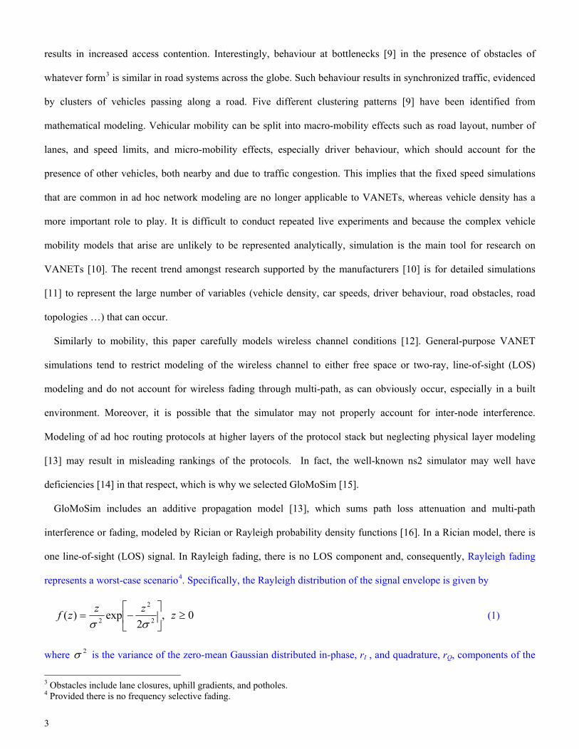
Similarly to mobility, this paper carefully models wireless channel conditions [12]. General-purpose VANET
simulations tend to restrict modeling of the wireless channel to either free space or two-ray, line-of-sight (LOS)
modeling and do not account for wireless fading through multi-path, as can obviously occur, especially in a built
environment. Moreover, it is possible that the simulator may not properly account for inter-node interference.
Modeling of ad hoc routing protocols at higher layers of the protocol stack but neglecting physical layer modeling
[13] may result in misleading rankings of the protocols. In fact, the well-known ns2 simulator may well have
deficiencies [14] in that respect, which is why we selected GloMoSim [15].
GloMoSim includes an additive propagation model [13], which sums path loss attenuation and multi-path
interference or fading, modeled by Rician or Rayleigh probability density functions [16]. In a Rician model, there is
one line-of-sight (LOS) signal. In Rayleigh fading, there is no LOS component and, consequently, Rayleigh fading
represents a worst-case scenario4. Specifically, the Rayleigh distribution of the signal envelope is given by
,2
exp)( 2
2
2 ⎥⎦
⎤⎢⎣
⎡−=
σσzzzf 0≥z (1)
where 2σ is the variance of the zero-mean Gaussian distributed in-phase, rI , and quadrature, rQ, components of the
3 Obstacles include lane closures, uphill gradients, and potholes. 4 Provided there is no frequency selective fading.

4
signal envelope:
)()()( 22 trtrtz QI += (2)
The Rician distribution is given by
,2
)(exp)( 202
22
2 ⎟⎠⎞
⎜⎝⎛
⎥⎦
⎤⎢⎣
⎡ +−=
σσσzsIszzzf 0≥z (3)
where the in-phase and quadrature components are no longer Gaussian, as there is a fixed LOS component. I0 is the
modified Bessel function of zeroth order. The average power in the non-LOS components is given by 22σ and s2 is
the power of the LOS component. The fading parameter 22 2σsK = is the ratio of these powers. In fact, the right-
hand-side of (3) can be rewritten in terms of K and the average received power [16]. If K = 0 then (3) reverts to a
Rayleigh distribution and with ∞=K there is only a LOS component. The Rayleigh distribution represents a
situation in which nodes are highly mobile. The restrictions of an urban topology make highly mobile nodes unlikely.
In communication, between vehicles in a city there will often be a LOS component, as vehicles will be aligned along
road segments and mobility is often restricted. We consider a Rician fading channel, as the Rician distribution
includes a LOS component. Setting K = 3 (or 4.7 dB) by default results in a moderate departure from the Rayleigh
distribution and, in fact, in many cases K does not exceed 7 dB [17].
Simulations may also mislead if they take no account of packet length by thresholding the Signal-to-Interference-
Noise Ratio (SINR) level rather than determining the Bit Error Rate (BER), which is a feature of GloMoSim but is
not present in ns2 [13]. Notice that signal reception thresholding is acceptable if all packets are long [13]. However,
the latter is not normally the case for video communication. GloMoSim also includes an additive node interference
model and does not use the capture threshold model of ns2, which is criticized in [18]. Therefore, in summary closer
modeling of wireless conditions in this paper includes in the results: 1) an additive node interference model; 2) fading
and a simple path loss model, as remains common; and 3) appropriate treatment of signal reception.
Packet losses are likely to be greater than those reported in simulation studies primarily concerned with protocol
development. The Scalable Video Coding (SVC) extension of H.264/Advanced Video Codec (AVC) [19] allows
lightweight creation of quality layers suitable for transport over multiple paths. A key problem with SVC is that there
are complex interdependencies between the layers. In particular, the base layer must arrive intact, before

5
reconstruction of enhancements layers can take place. At a cost in overhead, application layer FEC can be applied.
However, without knowledge of the FEC present at the PHY layer AP-FEC may simply overlap what is already
present. Alternatively, negative acknowledgements can be sent [20] but this only adds to the generally high end-to-
end delays in this type of network. Therefore, in this paper, though SVC remains a promising alternative, we
introduce spatial Multi-Description Coding (MDC) to counter the effect of packet loss on video streams. In MDC
[21], a video stream is decomposed into two or more descriptions, each of which is sufficient to reconstruct the video
sequence but both of which are required to reconstruct the video at good quality. MDC can be achieved through
temporal decomposition of the frame sequence [22] but this may lead to additional anchor frames or encoder-decoder
drift, unless specialist codecs are employed. Instead, we consider spatial decomposition. By employing checkerboard
Flexible Macroblock Ordering (FMO) [23], an error-resilience feature of the H.264/AVC [24], each frame can be
separated into two or more slices. These slices can aid the reconstruction of adjacent macroblocks in another slice in
the event of the packet bearing that slice being lost. Checkerboard FMO is the only one of the H.264/AVC FMO
types that has this property. To achieve reconstruction error, error concealment [25] at the decoder is necessary,
which might tax the processor available to a battery-powered device but is not a barrier to its use within a vehicle.
Therefore, the application of spatial FMO to MDC within a VANET is the final contribution of this paper.
Prior work by us [26] or by others [27] considered the possibility of combining overlay networks with mobile ad
hoc networks (MANETs) but did not considered an extension to VANETs, in which quite different mobility patterns
occur, different assumptions are made, such as the possibility of buffering, and more rigorous channel modeling is
necessary. The work in [27] applied the random waypoint model [28], typical of MANET modeling, to find routing
protocol performance under file download. The research employed a shadowing wireless model but, as the simulator
was ns2, a simple capture threshold was in use. The paper does, however, summarize prior work on overlays
combined with MANETs. Our work in [26], did consider MDC over the overlay but again this was in the context of
a MANET. However, the work in [26] for a MANET applied temporal MDC and not spatial MDC. This is
significant, as we now think spatial MDC is more efficient for the reasons outlined earlier. In other words, work with
temporal MDC may underestimate the ability to stream video. In [29], simple temporal splitting occurred with the
simulation environment the same as that of [27]. In fact, in what may be termed the pioneering stage of ad hoc
networks, there was considerable investigation of video streaming [30] but the simulation environments were

6
simplified. For example, in [31] the inadequacy of general-purpose MANET mobility modeling for VANETs is
highlighted. The FMO facility of H.264/AVC is giving rise to a number of ways of exploiting spatial MDC. The
closest work to our use of spatial FMO was independently outlined in [32]. However, the analysis in [32] was for a
very general mobile environment and only examined the resulting video quality. As a further example, in [33], FMO
is used to isolate regions of interest (ROIs), while redundant slices are sent to protect the ROI. A problem with this
scheme may indeed be the extra data sent in the redundant slices, while checkerboard FMO does not entail such
overheads or the need to identify ROIs.
Therefore, our work represents a realistically modeled scheme for streaming video over a VANET, by means of an
overlay network with multi-sources. In combining spatial FMO, MDC, VANET, and overlay, it most likely arrives at
a unique combination. As such it demonstrates a way forward for ‘infotainment’ within automotive networks, which
are a growing sector of the wireless communications industry.
2. Overlay network streaming Fig. 1 illustrates an application overlay functioning within a VANET, in which the overlay network is mapped onto
the physical network. Thus, the overlay node placement is logically different to that of the physical placement of the
nodes. We simulate a mesh architecture with all-to-all connectivity [7], Fig. 2. This approach is more robust than a
tree-based architecture, because, when a stream comes from various sources, communication does not break-down
when a subset of peers disconnects. In the example scenario illustrated, seven nodes form a mesh within which two
nodes are the original source nodes for the same video. A likely way that two nodes in a VANET could acquire the
same video clip is that both could have passed a roadside unit offering informational/advertising video clips.
However, it is also possible that these two nodes previously could have acquired the same video from a single node,
prior to the distribution process illustrated in Fig. 2. Three nodes (node C, node D and node E) receive video from
these two source nodes. The three nodes in turn also act as sources to two further nodes (node F and node G). Hence,
nodes C, D and E download and upload at the same time i.e. act as receivers and sources at the same time. All
receiving nodes, C to G, are served by multiple sources. Moreover in Fig. 2, nodes F and G can receive data from an
alternative source if a source ceases to be available.

7
Figure 1. An example of an application overlay over VANET (after [27])
Figure 2. Mesh-based overlay topology sending video streams from sources to receivers (after [27])
Peer selection for streaming purposes can either be achieved in one of three ways. Firstly, it is achieved in a
hybrid fashion, by including some server nodes in the manner of commercial P2P streaming. Secondly, a structured
overlay can be organized that allows quicker discovery of source peers than in an unstructured overlay. However,
structured overlays require the source data to be placed in particular nodes, which may not be practical in a VANET.
Therefore, we assume an unstructured and decentralized overlay such as Gnutella, KaZaa, or GIA [34].

8
3. Modeling a VANET
3.1 Simulation settings We employed the Global Mobile System Simulator (GloMoSim) [15] simulation library to generate results.
GloMoSim as developed by the authors of [15] is based on a layered approach similar to the OSI seven-layer network
architecture. For video transport IP framing was employed with UDP transport, as TCP transport can introduce
unbounded delay, which is not suitable for delay-intolerant video streaming. The default network configuration
consisted of seven nodes forming an overlay network, as arranged in Fig. 2, with these nodes selected from a total of
100 nodes (vehicles) forming the complete VANET. GloMoSim was altered so that nodes start at random locations
rather than at the origin, to avoid biased results.
3.2 Default radio environment IEEE 802.11p [4] has four 10 MHz service channels suitable for video streaming, with other channels dedicated to
control and safety applications. Receiver sensitivity in the simulation was set to -92 dBm. IEEE 802.11p’s Binary
Phase Shift Keying (BPSK) modulation mode with 1/2 coding rate was simulated. Accordingly, the data-rate was set
to 3 Mbps. (Request to Send / Clear to Send) (RTS/CTS) signaling was turned on. As a default, a two-ray path loss
model with an omni-directional antenna height of 1.5 m at receiver and transmitter was selected for which the
reflection coefficient was -0.7, which is the same as that of an asphalt road surface. The plane earth path loss
exponent was set to 4.0, with the direct path exponent set for free space propagation (2.0). In IEEE 802.11p
transmission is at 5.9 GHz, when the two-ray crossover distance is about 556.5 m, which is calculated from (4).
λπ rt
crosshh
d4
= (4)
where ht and hr are the transmitter and receiver antenna heights respectively, and λ is the transmission wavelength.
3.3 Mobility modeling In VanetMobiSim [35], as used by us, a variety of urban road layouts can be generated of increasing density by
means of the random backbone mode using Voronoi tessellations. In the simulations, a square 1000 m2 area was
defined and nodes (vehicles) were initially randomly placed within the area. Other spatial settings to do with road
clusters, intersection density, lanes (2) and speeds are given in Table I. The number of clusters refers to the number

9
of rectangular areas with a road density of 2 obstacles/ 100 m2 (2e-4) for the Downtown model (to create randomly a
non-homogeneous simulation terrain), while the remainder of the terrain is at the minimum road density, which was
the same as that for a residential area, i.e. 2e-5. The number of traffic lights (at intersections) and time intervals
between changes are also defined. In the following paragraph, the equation variable annotations in Table 1 are
identified, with some uncommented terms explained at the end of this Section. These values in Table 1 were the
defaults for VanetMobiSim.
The real advantage of VanetMobiSim is the variety of driver behaviour models. A summary of mobility
configurable settings applied in the simulations is also given in Table 1. The Constant Speed Motion (CSM), the
simplest of these, does not produce realistic motions (as it is possible for vehicles to overlap during motion) and is
included for comparison with earlier results in other papers. In this model the speed of each vehicle is determined on
the basis of the local state of each car and any external effect is ignored. A vehicle follows a random movement
(across the road topology) in the sense that a destination is selected and vehicle moves towards it, possibly pausing at
intersections. In the Fluid Traffic Model (FTM), the traffic density affects a vehicle’s speed. This model describes the
vehicle’s speed as a monotonically decreasing function of the traffic density. When traffic congestion reaches a
critical state, then the node speed is constrained by (5).
⎥⎥⎦
⎤
⎢⎢⎣
⎡⎟⎟⎠
⎞⎜⎜⎝
⎛−=
jamkksss 1,max maxmin (5)
where s is the output speed, smin and smax are minimum and maximum speed constraints respectively, kjam is the
vehicular density at which a traffic jam is declared, and k is the current vehicle density of the road the vehicle of
interest is moving on. lnk = , where n is the number of vehicles on that road and l is the length of the road.
The Intelligent Driver Model (IDM) accords with car-following model [9] based on live observations. The
instantaneous acceleration of a vehicle is computed by (6).
⎥⎥⎦
⎤
⎢⎢⎣
⎡⎟⎠⎞
⎜⎝⎛−⎟⎟
⎠
⎞⎜⎜⎝
⎛−=
24
0
*1s
svva
dtdv (6)
where a is the maximum acceleration of the vehicle, v is the current speed of the vehicle, v0 is the desired velocity, s
is the distance from the preceding vehicle and s* is a desired dynamical distance, as given by (7).

10
abvvvTss
2* 0
Δ++= (7)
where s0 is the minimum desirable bumper-to-bumper distance, and T is the minimum safe time between two
vehicles. The speed difference with respect to front vehicle velocity is ∆v, and the normal de-acceleration rate is b.
VanetMobiSim modifies IDM by modeling intersection management (IDM-IM) as a lead vehicle approaches an
intersection. Whenever a vehicle approaches an intersection with stop signs or traffic lights the parameters in (8) are
used in IDM-IM to set its speed.
⎩⎨⎧
=Δ−=vvSs σ
(8)
where σ is now the current distance to the intersection and S is a safety distance, as the vehicle does not stop exactly
at the intersection. Once the vehicle is halted at the intersection detailed behaviour, which depends on other vehicles
on other roads leading into the intersection and the state of the traffic lights if present, is described in [35]. The IDM-
IM includes lane change behaviour in the IDM-LC model. At intersections, if a lane ceases to exist on the other side
of the intersection, a vehicle will wait until a gap appears. More generally, for overtaking using lanes, a game-
theoretical model [36] is applied. A lane change will occur if the advantage of a vehicle changing lanes to a new lane
is greater than the disadvantage to following vehicles in the current lane and the new lane. This is measured in terms
of acceleration, a, by inequalities (9) and (10).
thrlnew
lcurnewcurbias
l aaaaapaaa +−−−>±− )( (9)
safelnew aa −> (10)
Thus (al- a) is the gain in acceleration from moving o lane l, with similar expressions for the loss in acceleration for a
following vehicle in the current lane and the new lane (when the lane swapping vehicle joins it). p is a driver
politeness factor, abias is a lane bias factor encouraging lane changes to a particular side, and asafe restricts movements
avoid a driver in the new lane having to decelerate too quickly as a result of the lane change. The term athr is a
minimum acceleration below which lane changing has limited value. The values of some of these parameters can be
found in Table 1.
In Table 1, “Recalculation of movement parameters interval” is the interval after which the simulator recalculates
parameters and makes a decision on those parameters. This time interval does not have a direct impact on the

11
simulation time but indicates the update frequency. In the CSM model, pause time is set to zero because, unlike in a
general ad hoc network, it is not expected that a vehicle will malinger for any reason. The minimum and maximum
stay times are times spent parking or stopping for any reason. These are set to low values by default.
Therefore, the micro-mobility models presented by VanetMobiSim are of increased sophistication in driver
behaviour. Notice though that when driver behaviour is introduced into simulations it is no longer possible to easily
examine node speed dependencies, as the vehicles will have a range of speeds depending on local conditions, even
though the minimum and maximum speeds are not exceeded.
Table 1. VanetMobiSim configurable settings with road layout and mobility models
Global Parameters Terrain dimension 1000 m2 Graph type Space graph
(Downtown model) No. of road clusters 4 Min. intersection density 2e-5 Max. traffic lights 6 Time interval between traffic lights change
10 s
Number of lanes 2 Min. stay 10 s Max. stay 100 s Nodes (vehicles) 50, 100 Min. speed (smin) 3.2 m/s (7 mph) Max. speed (smax) 13.5 m/s (30 mph) CSM model Min. and max. pause time 0 s FTM Model Density of traffic jam 0.2 cars/m Recalculation of traffic parameters interval
0.1 s
IDM Model, IDM-IM Model, IDM-LC Model Length of vehicle 5 m Max. acceleration (a) 0.6 m/s2 Normal deceleration (b) 0.5 m/s2 Traffic jam distance 2 m Node’s safe time headway (T) 1.5 s Recalculation of movement parameters interval
0.1 s
Other Parameters of IDM-LC Model Safe deceleration (asafe) 4 m/s2 Politeness factor of drivers when changing lane (p)
0.5
Threshold acceleration for lane change (athr)
0.2 m/s2
12
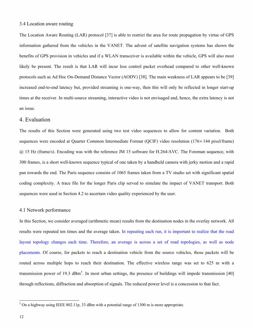
3.4 Location aware routing
The Location Aware Routing (LAR) protocol [37] is able to restrict the area for route propagation by virtue of GPS
information gathered from the vehicles in the VANET. The advent of satellite navigation systems has shown the
benefits of GPS provision in vehicles and if a WLAN transceiver is available within the vehicle, GPS will also most
likely be present. The result is that LAR will incur less control packet overhead compared to other well-known
protocols such as Ad Hoc On-Demand Distance Vector (AODV) [38]. The main weakness of LAR appears to be [39]
increased end-to-end latency but, provided streaming is one-way, then this will only be reflected in longer start-up
times at the receiver. In multi-source streaming, interactive video is not envisaged and, hence, the extra latency is not
an issue.
4. Evaluation The results of this Section were generated using two test video sequences to allow for content variation. Both
sequences were encoded at Quarter Common Intermediate Format (QCIF) video resolution (176×144 pixel/frame)
@ 15 Hz (frame/s). Encoding was with the reference JM 15 software for H.264/AVC. The Foreman sequence, with
300 frames, is a short well-known sequence typical of one taken by a handheld camera with jerky motion and a rapid
pan towards the end. The Paris sequence consists of 1065 frames taken from a TV studio set with significant spatial
coding complexity. A trace file for the longer Paris clip served to simulate the impact of VANET transport. Both
sequences were used in Section 4.2 to ascertain video quality experienced by the user.
4.1 Network performance In this Section, we consider averaged (arithmetic mean) results from the destination nodes in the overlay network. All
results were repeated ten times and the average taken. In repeating each run, it is important to realize that the road
layout topology changes each time. Therefore, an average is across a set of road topologies, as well as node
placements. Of course, for packets to reach a destination vehicle from the source vehicles, those packets will be
routed across multiple hops to reach their destination. The effective wireless range was set to 625 m with a
transmission power of 19.3 dBm5. In most urban settings, the presence of buildings will impede transmission [40]
through reflections, diffraction and absorption of signals. The reduced power level is a concession to that fact.
5 On a highway using IEEE 802.11p, 33 dBm with a potential range of 1300 m is more appropriate.

13
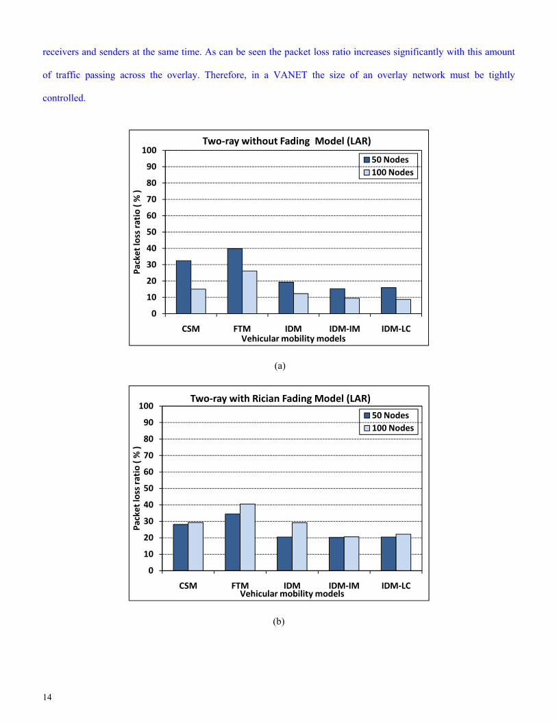
In Fig. 3a, the packet loss ratios (ratio of packets sent to packets lost) would make unprotected streaming of video
feasible in the denser network if lane changing was permitted, as losses below 10% occur in that scenario. It is
possible that for packet loss rates up to 20% but no more than 30% (see Section 4.2), inclusion of error resilience or
application-layer forward error correction could compensate for high packet loss rates. Fig. 3a shows that more
careful modeling of driver behaviour can actually decrease the predicted level of packet loss (going from CSM to
IDM-LC). However, lane-changing (IDM-LC) which allows increased mobility is not always possible within a city.
A feature of Fig. 3b and 3c is that more careful wireless channel modeling results in a drop in packet loss.
However, the introduction of fading models causes the simulator to report greater packet losses in the denser network
(100 nodes). This is because, when path loss only is modeled, then the distance between nodes is the principal effect
and the sparser network (50 nodes) results in greater losses. However, if the nodes are closer together then
interference at road obstacles due to traffic queuing increases the number of packet losses. In addition, both sparse
and dense networks suffer from additional packet loss from fading. Fig. 4 varies the fading parameter or factor K
arising from the Rician distribution for reasonable values of K [17] with the IDM-IM mobility model. When K is
lower than 3, then an increase in packet loss occurs and the packet loss behaviour begins to resemble that for the
Rayleigh distribution, Fig. 3c. When K is higher than the default value of 3, the increasing dominance of the LOS
component means that the packet loss regime depends more on the LOS component. As K reaches 6 (7.8 dB) then the
sparser network begins to suffer more packet losses, perhaps because of a relative increasing impact of path loss
rather than fading.
The impact of cross-traffic on packet loss was assessed. Four nodes that were not part of the overlay were
introduced, each sending 100 packets of packet length 400 bytes as a CBR stream, again with the IDM-IM mobility
model for Rician fading with K = 3. Such messages could represent text safety alerts. From Table *, it is apparent
that moderate cross traffic does not greatly affect the packet loss ratios, though it might prove important to video
quality as the losses reach above 20% (as it is difficult to reconstruct even with error resilience once losses reach
above 20%). However, varying the overlay size certainly does have a significant effect on packet loss ratios. In the
‘More Peers’ scenario of Table 2, a total of 14 peers were part of the overlay. Two peers were source peers initially
and six peers acted as receivers. These same six peers served four more peers. These four peers sent streams to two
more peers. These means that 12 peers acted as source and 12 peers were receivers. Amongst these ten peers acted as
14
receivers and senders at the same time. As can be seen the packet loss ratio increases significantly with this amount
of traffic passing across the overlay. Therefore, in a VANET the size of an overlay network must be tightly
controlled.
0
10
20
30
40
50
60
70
80
90
100
CSM FTM IDM IDM-IM IDM-LC
Pack
et lo
ss ra
tio
( % )
Vehicular mobility models
Two-ray without Fading Model (LAR)
50 Nodes100 Nodes
(a)
0
10
20
30
40
50
60
70
80
90
100
CSM FTM IDM IDM-IM IDM-LC
Pack
et lo
ss ra
tio
( % )
Vehicular mobility models
Two-ray with Rician Fading Model (LAR)
50 Nodes100 Nodes
(b)

15
0
10
20
30
40
50
60
70
80
90
100
CSM FTM IDM IDM-IM IDM-LC
Pack
et lo
ss ra
tio
( % )
Vehicular mobility models
Two-ray with Rayleigh Fading Model (LAR)
50 Nodes100 Nodes
(c)
Figure 3. Packet loss ratio compared by mobility model for different network sizes for (a) no fading, (b) Rician fading, and (c) Rayleigh fading, with routing by the LAR protocol
0
5
10
15
20
25
30
35
40
45
50
2 3 4 5 6 7
Pack
et lo
ss ra
tio
( % )
Rician K factor values
50 Nodes100 Nodes
Figure 4. Packet loss ratio with Rician fading and varying K factor for an IDM-IM mobility model and LAR routing
Table 2. Packet loss ratios when either introducing cross-traffic or more peers into the overlay for an IDM-IM mobility model, Rician fading model with K = 3, and LAR routing.
Scenarios Cross Traffic More Peers 50 Nodes 22.22% 45.75% 100 Nodes 21.45% 46.43%

16
As might be expected, when the node density increases, then end-to-end-delay increases. The number of hops
traversed by a packet increases on average, resulting in longer delay. This is illustrated by the differences between
the results for different network sizes, Fig. 5, for the original overlay scenario with seven nodes. However, an
interesting feature of these results is that more realistic modeling actually indicates that the delay for the sparser
networks is less than predicted by the coarser mobility models. That is the effect of network sparseness is equalized
to some extent when the effects of driver behaviour are taken into account. For the denser network of 100 nodes,
delay is forecast to be less under a two-ray model. When fading is taken into account, Fig. 5b, c, then predicted delay
increases. At the levels of delay reported, one-way video streaming is the main option but this is not a problem as
overlay network applications are generally not interactive. Therefore, the main role of estimating the delay is to assist
in buffer dimensioning, which for the Paris video stream at 15 Hz obviously requires about a 45 frame buffer. The
size of the buffer will affect start-up delay experienced by the user. If the user consciously selects a clip then delay
will be perceptible, as it is not below 250 ms and ideally about 100 ms. If delivery is automatic, e.g. in a congestion
monitoring application, then the user will not be aware of the start time of streaming.
0
2
4
6
8
10
12
CSM FTM IDM IDM-IM IDM-LC
Ave
rage
end
-to-
end
dela
y ( s
)
Vehicular mobility models
Two-ray without Fading Model (LAR)
50 Nodes100 Nodes
(a)

17
0
2
4
6
8
10
12
CSM FTM IDM IDM-IM IDM-LC
Ave
rage
end
-to-
end
dela
y ( s
)
Vehicular mobility models
Two-ray with Rician Fading Model (LAR)
50 Nodes
100 Nodes
(b)
0
2
4
6
8
10
12
CSM FTM IDM IDM-IM IDM-LC
Ave
rage
end
-to-
end
dela
y ( s
)
Vehicular mobility models
Two-ray with Rayleigh Fading Model (LAR)
50 Nodes
100 Nodes
(c)
Figure 5. End-to-end delay compared by mobility model for different network sizes for (a) no fading, (b) Rician fading, and (c) Rayleigh fading, with routing by the LAR protocol
Fig. 6 considers the efficiency of the routing process by charting the per-packet control packet overhead. The LAR
protocol has reduced the levels of overhead below those normally experienced. However, when fading is present
overhead does increase. There is also an energy consumption implication, as transmission for a battery-driven device
can consume as much as 80% of the energy. However, for VANETs, assuming the transceivers are re-chargeable
from the engine’s alternator, there is not such an implication.

18
0
0.1
0.2
0.3
0.4
0.5
0.6
0.7
0.8
0.9
1
CSM FTM IDM IDM-IM IDM-LC
Cont
rol o
verh
ead
( pac
kets
)
Vehicular mobility models
Two-ray without Fading Model(LAR)
50 Nodes100 Nodes
(a)
0
0.1
0.2
0.3
0.4
0.5
0.6
0.7
0.8
0.9
1
CSM FTM IDM IDM-IM IDM-LC
Cont
rol o
verh
ead
( pac
kets
)
Vehicular mobility models
Two-ray with Rician Fading Model (LAR)
50 Nodes100 Nodes
(b)

19
0
0.1
0.2
0.3
0.4
0.5
0.6
0.7
0.8
0.9
1
CSM FTM IDM IDM-IM IDM-LC
Cont
rol o
verh
ead
( pac
kets
)
Vehicular mobility models
Two-ray with Rayleigh Fading Model(LAR)
50 Nodes100 Nodes
(c)
Figure 6. Control overhead in packets for different mobility models with 50 and 100 nodes with two-ray propagation path-loss model with (a) no fading, (b) Rician fading, and (c) Rayleigh fading, with routing by the LAR protocol
4.2 Video performance
We considered the consequences of applying spatial multi-description coding to the dual streams. For FMO error
resilience [23], compressed frame data is normally split into a number of slices each consisting of a set of
macroblocks [41]. Slice resynchronization markers ensure that if a slice is lost then the decoder is still able to
continue with entropic decoding. Therefore, a slice is a unit of error resilience and it is normally assumed that one
slice forms a packet, after packing into a Network Abstraction Layer unit (NALU) in H.264/AVC [24]. Each NALU
is further encapsulated by a Real-Time Protocol (RTP) header [42] within an IP/UDP packet, resulting in an
additional 40 bytes. For comparison purposes, one simple form of spatial ‘MDC’ is to employ slicing (without FMO)
in which the top part of the encoded frame forms one slice and the bottom half forms the other slice. Then each set of
slices (top and bottom) form a description but these cannot be used to reconstruct the other if the packet bearing that
slice is lost. Instead, previous frame replacement must be employed by the decoder.
In checkerboard FMO, the macroblocks equivalent to the white squares of a checker or chess board form one
slice while the remaining macroblocks form the other slice. Error concealment is a non-normative feature of
H.264/AVC. In our experiments, the motion vectors of macroblocks from correctly received slices are utilized to
reconstruct macroblocks from missing FMO slices. This takes place if the average motion activity is sufficient (more

20
than a quarter pixel). Research in [25] gives details of which motion vector to select to give the smoothest block
transition. It is also possible to select the intra-coded frame method of spatial interpolation, which provides smooth
and consistent edges at an increased computational cost. However, temporal error concealment is preferable, unless
‘high motion activity’ or scene cuts are present. The method of concealment can be selected depending on the
smoothness of reconstructed macroblock border transitions. As the lower complexity H.264 Baseline Profile was
employed the Group of Pictures [41] frame structure was IPPPPP…To reduce error propagation both MDC schemes
employed Gradual Decoder Refresh [24] by insertion of an intra-coded row of macroblocks into each encoded frame,
cycling the replaced row through the video sequence.
In Fig. 7, packet losses at rates up to 30% were generated from a Uniform distribution and the Peak Signal-to-
Noise Ratio (PSNR) was calculated. PSNR is given by (11).
PSNR =( )
⎥⎥⎥⎥
⎦
⎤
⎢⎢⎢⎢
⎣
⎡
−∑∑i j
recref
peak
jiYjiYN
V210
)),(),((1log20 (11)
where ),( jiYref and ),( jiYrec are the reference and reconstructed pixels respectively, with I and j ranging over the
rows and columns of the frame. The reference is taken to be the raw video prior to encoding. N is the total number of
pixels in that frame and Vpeak is the peak pixel value of a pixel with 8-bit resolution, i.e. 255.
To ensure convergence each data point was the mean of fifty tests. From the Figure it is apparent that apart from
zero packet loss, simple slicing (MDC) fares badly in comparison to checkerboard FMO with MDC (MDC with
Error Res.). At zero packet loss the extra overhead from including the FMO macroblock mapping in a packet results
in a drop in quality (if the datarate is the same as for simple slicing). However, from 8% packet loss onwards, the
video quality for both sequences using simple slicing would be unacceptable. For Paris, the video quality using
checkerboard FMO in conjunction with error concealment results in reasonable video quality. Though the PSNR
drops below 30 dB, it is generally the case that users will tolerate PSNRs above 25 dB for mobile applications. In
fact, it is possible to equate PSNR to the ITU-R’s Mean Opinion Scores [29], when the range 25 to 31 dB inclusive
is approximately equivalent to a score of 3 or “fair” (from a range 1 to 5 with 5 being “excellent”. For Foreman, the
drop in quality is steeper reflecting the more complex source coding task. However, below 20 % packet loss ratio, the

21
quality would be tolerable. From Fig. 3b, this occurs under Rician channel conditions and IDM models when there
are fifty vehicles in the network.
0
5
10
15
20
25
30
35
0 8 9 12 15 16 19 20 21 22 26 28 29 30
PSN
R (d
B)
Loss ratio (%)
MDCMDC with Error Res.
(a)
0
5
10
15
20
25
30
35
40
0 8 9 12 15 16 19 20 21 22 26 28 29 30
PSN
R (d
B)
Loss ratio (%)
MDCMDC with Error Res.
(b)
Figure 7. Applying MDC with and without error resilience to dual path video streaming of (a) the Foreman sequence, (b) the Paris sequence.
5. Concluding remarks
As the integration of wireless networks takes place, it is likely that multimedia exchange will spread to VANETs.

22
Some high-end cars already include WLAN capability and the advantages that the emerging IEEE 802.11p standard
will bring for traffic safety will encourage manufacturers further in that direction. Video streaming has advantages
over download in terms of regulated bandwidth usage, reasonable start-up delay for longer sequences, and
commercial confidentiality. Multi-source streaming across an overlay networks is potentially a robust form of video
delivery. However, the size of such overlays will need to be strictly controlled in a VANET to prevent an increase in
competing traffic amongst the overlay nodes, leading to unacceptable increases in packet loss ratios. This paper has
shown that more realistic mobility and driver behaviour modeling, along with probabilistic fading models causes
considerable differences in reported packet loss ratios, even with a reasonable number of nodes. Nevertheless, the
spatial MDC method introduced in this paper is able to counter adverse conditions present in a VANET.
References
[1] Jajubiak, J., and Koucheryavy, Y.: ‘State of the art and research challenges for VANETs’, Proc. IEEE Consumer
Commun. and Networking Conf., Las Vegas, NV, USA, Jan. 2008, pp. 912-916.
[2] Wu, H., Qiao, C., De, S. and Tonguz, O: ‘Integrated cellular and ad hoc relaying service: iCAR’, IEEE J. on Sel.
Areas in Communs., 2001, 19, (10), pp. 2105-2113.
[3] Guo, M., Ammar, M. H., and Zegura, E. W.: ‘V3: A vehicle-to-vehicle live video streaming architecture’, Proc.
3rd IEEE Int. Conf. on Pervasive Computing and Communs., Kauai Island, HI, USA, Mar. 2005, pp. 171-180.
[4] Jiang, D. and Delgrossi, L.: ‘IEEE 802.11p: Towards an international standard for wireless access in vehicular
environments’, Proc. IEEE Vehicular Technol. Conf., Singapore, May 2008, pp. 2036-2040
[5] Yan, L.: ‘Can P2P benefit from MANET? Performance evaluation from users' perspective’, Proc. Int. Conf. on
Mobile Sensor Networks, Limassol, Cyprus, Jun. 2005, pp. 1026-1035
[6] Zheng, W., Liu, X., Shi, S., Hu, J. and Dong, H.: ‘Peer-to-peer: A technical perspective’, in Wu, J. (ed.):
‘Handbook on Theoretical and Algorithmic Aspects of Sensor, Ad Hoc Wireless, and Peer-to-Peer Networks’,
Wu, J. (Ed.), (Auerbach Pubs., 2006), pp. 591-615
[7] Yong, L., Guo, Y., and Liang, C.: ‘A survey on peer-to-peer video streaming systems’, Peer-to-Peer Networking
and Applications, 2008, 1, pp. 18-28
23
[8] Universität of Bonn, ‘BonnMotion: A Mobility Scenario Generation and Analysis Tool’, User Manual, June 10,
2009
[9] Treiber, M., Henneke, A., and Helbing, D.: ‘Congested traffic states in empirical observations and microscopic
simulations’, Phys. Rev. E, Aug. 2000, 62, (2), pp. 1805-1824.
[10] Tonguz, O. K., Viriyasitavat, W. and Bai, F.: ‘Modeling urban traffic: A cellular automata approach’, IEEE
Communs. Mag., May 2009, 47, (5), pp. 142-150
[11] Liu, B., Khorashadi, B., Du, H., Ghosal, D., Chuah, C.-N., and Zhang, M.: ‘VGSim: An integrated
networking and microscopic vehicular mobility simulation platform’, IEEE Communs. Mag., May 2009, 47, (5),
pp. 134-141
[12] Matolak, D.W.: ‘Channel modeling for vehicle-to-vehicle communications’, IEEE Communs. Mag., May
2008, 46, (5), pp. 76-83.
[13] Takai, M., Martin, J., and Bagrodia, R.: ‘Effects of wireless physical layer modeling in mobile ad hoc
networks’, Proc. Int. Symp. on Mobile Ad Hoc Networking and Computing, Chicago, USA, 2001, pp. 87-94
[14] Wellens, M., Petrova, M., Riihijärvi, J., and Mähönen, P.: ‘Building a better mousetrap: Need for more
realism in simulation’, Proc. 2nd Ann. Conf. on Wireless on Demand Network Syst. and Services, St. Moritz,
Switzerland, Jan. 2005, pp. 150-157
[15] Zeng, X., Bagrodia, R., and Gerla, M.: ‘GloMoSim: A library for parallel simulation of large-scale wireless
networks’, Proc. 12th Workshop on Parallel and Distributed Simulations, Banff, Canada, May 1998, pp. 154-161
[16] Goldsmith, A.: ‘Wireless Communications’, (Cambridge University Press, 2005)
[17] Doukas, A., and Kalivas, G.: ‘Rician K factor estimation for wireless communication systems’, Proc. IEEE
Int. Conf. on Wireless and Mobile Communs., Bucharest, Romania, Jul. 2006, pp. 69-73
[18] Iyer, A., Rosenburg, C. and Karnik, A.: ‘What is the right model for wireless channel interference?’, IProc.
3rd Int. Conf. on QoS in Heterogeneous Wired/Wireless Networks, 2006, Ontario, Canada, Article no. 2
[19] Schwartz, H., Marpe, D., and Wiegand, T.: ‘Overview of the scalable video coding extension of the
H.264/AVC standard’, IEEE Trans. Circuits Syst. Video Technol., 2007, 17, (9), pp. 1103-1120

24
[20] Mao, S., Lin, S., Panwar, S. S., Wang, Y., and Celebi. E.: ‘Video transport over ad hoc networks:
multistream coding with multipath transport’, IEEE J. on Sel. Areas in Communs., 2003, 21, (4), pp. 1721-1737
[21] Wang, Y., Reibman, A. R. and Lin, S.: ‘Multiple description coding for video delivery’, Proceedings of the
IEEE, Jan. 2005, 93, (1), 57-70
[22] Apostolopoulos, J.: ‘Reliable video communication over lossy packet networks using multiple state
encoding and path diversity’, Visual Comms.: Image Processing, Jan. 2001, 392-409
[23] Lambert, P, de Neve, W., Dhondt, Y. and Van de Walle, R.: ‘Flexible macroblock ordering in H.264/AVC’,
J. of Visual Communication and Representation, Apr. 2004, 17 , (2), 358-378
[24] Wenger, S.: ‘H264/AVC over IP’, IEEE Trans. Circ. Syst. Video Technol., July 2003, 13, (7), pp. 645-656
[25] Vars, V. and Hannuksela, M. N.: ‘Non-normative error concealment algorithms’, ITU-T SGI6 Doc., VCEG-
N62, 2001
[26] Qadri, N., Altaf, M., Liotta, A., Fleury, M., and Ghanbari, M., ‘Effective video streaming using mesh P2P
with MDC over MANETS’, J. of Mobile Multimedia, 2009, 5, (4), pp. 301-317
[27] Oliveira, L. B., Siqueira, I.G. and Loureiro, A.A.F.: ‘On the performance of ad hoc routing protocols under a
peer-to-peer application’, J. of Parallel and Distributed Computing, 2005, 65, (11), pp. 1337-1347
[28] Broch, J., Maltz, D.A., Johnson, D.B. et al.: ‘A performance comparison of multi-hop wireless ad hoc
network routing protocols’, Proc. ACM MOBICOM, Dallas, Texas, USA, Oct. 1998, pp. 85-97
[29] Chow, C.-O. and Ishii, H., ‘Enhancing real-time video streaming over mobile ad hoc networks using
multipoint-to-point communication’, Computer Communications, 2007, 30, pp. 1754-1764
[30] Zhang, Q.: ‘Video delivery over wireless multi-hop networks’, Proc. Int. Symp. on Intelligent Signal Proc.
and Commun. Syst., Dec. 2005, pp. 793-796
[31] Djenouri, D., Nekka, E. and Soualhi, W.: ‘Simulation of mobility models in vehicular ad hoc networks’,
Proc. ACM Int. Conf. on Ambient Media and Systs., Quebec, Canada, Feb. 2007, article no. 4
[32] Lamy-Bergot, C., Candillon, B., Pesquet-Popescu, B. and Gadat, B.: ‘A simple, multiple description coding
scheme for improved peer-to-peer video distribution over mobile links’, Proc. IEEE Packet Coding Symposium,
Chicago, USA, Apr. 2009.

25
[33] Yang, J. and Gong, S.: ‘A content-based layered multiple description coding scheme for robust video
transmission over ad hoc networks’, Proc. IEEE Int. Symp. on Elec. Commerce and Security, 2009, pp.21-24
[34] Chawathe, Y., Ratnasamy, S., Breslau, L., Lanham, N. and Shenker, S.: ‘Making Gnutella-like P2P systems
scalable’, Proc. of ACM SIGCOMM, Aug. 2003, pp. 407–418
[35] Fiore, M., Härri, J., Filali, F., and Bonnet, C.: ‘Vehicular mobility simulation for VANETs’, Proc. 40th Ann.
Simulation Symp., Norfolk, VI, USA, Mar. 2007, pp. 301-307
[36] Kesting, A., Treiber, M., and Helbing, D.: ‘General lane-changing model MOBIL for car-following models’,
Transportation Research Record, 2007, 1999, pp. 86-94
[37] Ko, Y. B., and Vaidya, N. H.: ‘Location-Aided-Routing (LAR) in mobile ad-hoc networks’, Proc.
ACM/IEEE MOBICOM, Dallas, Texas, USA, Oct. 1998, pp. 66-75
[38] Perkins, C. E., and Royer, E.M., ‘Ad Hoc On-Demand Distance Vector routing’, Proc. IEEE Workshop on
Mobile Computing Syst. and Applications, New Orleans, USA, Feb. 1999, pp. 90-100
[39] Qadri, N. N., and Liotta, A.: ‘A comparative analysis of routing protocols for MANETs’, Proc. IADIS Int.
Conf. on Wireless Applications and Computing, Amsterdam, Holland, Nov. 2008
[40] Oishi, J., Asukura, K., and Watanabe, T.: ‘A communication model for inter-vehicle communication
simulation systems based on properties of urban areas’, Int. J. of Computer Science and Network Security, 2006,
6, (10), pp. 213-219
[41] Ghanbari, M.: ‘Standard Codecs: Image Compression to Advanced Video Coding’, (IET Press, Stevenage,
UK, 2003)
[42] Wenger, S., Hannuksela, M.M., Stockhammer, T., Westerlund, M. and Singer, D.: ‘RTP payload format for
H.264’, RFC 3984, Feb. 2005
Top Related