


Languages
Pages
Legal


APPLYING GENERATIVE ADVERSARIAL NETWORKS TO
INTELLIGENT SUBSURFACE IMAGING
AND IDENTIFICATION
By
William Rice
Dr. Dalei WuProfessor of Computer Science(Chair)
Dr. Li YangProfessor of Computer Science(Committee Member)
Dr. Yu LiangProfessor of Computer Science(Co-Chair)

APPLYING GENERATIVE ADVERSARIAL NETWORKS TO
INTELLIGENT SUBSURFACE IMAGING
AND IDENTIFICATION
By
William Rice
A Thesis Submitted to the Faculty of the University ofTennessee at Chattanooga in Partial
Fulfillment of the Requirements of the Degreeof Master of Science: Computer Science
The University of Tennessee at ChattanoogaChattanooga, Tennessee
May 2019
ii
ABSTRACT
To augment training data for machine learning models in Ground Penetrating Radar (GPR)
data classification and identification, this thesis focuses on the generation of realistic GPR
data using Generative Adversarial Networks. An innovative GAN architecture is proposed for
generating GPR B-scans, which is, to the author’s knowledge, the first successful application
of GAN to GPR B-scans. As one of the major contributions, a novel loss function is
formulated by merging frequency domain with time domain features. To test the efficacy of
generated B-scans, a real time object classifier is proposed to measure the performance gain
derived from augmented B-Scan images. The numerical experiment illustrated that, based on
the augmented training data, the proposed GAN architecture demonstrated a significant
increase (from 82% to 98%) in the accuracy of the object classifier.
iii

ACKNOWLEDGEMENTS
To begin, I would like to acknowledge my wife, Shannon, she was here for all of the ups,
downs, and how every new project is ”The hardest problem I’ve ever solved”. I could not have
made it this far without her by my side. Furthermore, I would like to thank Dr. Wu, Dr. Liang,
and everyone in the lab for giving me the opportunity to conduct research in an academic
environment and facilitate my growth as a researcher. In addition, I would like to thank Mike
Tatum, Brent Spell, Josh Ziegler, and the rest of the team at Pylon ai. From the very beginning
they challenged me, which enabled me to grow in the field of machine learning. Without
them, I would not have been able to undertake a research project as challenging as this. I also
would like to include a special thank you to my thesis committee. The road to defense has
been rocky, but we finally made it.
iv

TABLE OF CONTENTS
ABSTRACT...............................................................................................................................iii
ACKNOWLEDGEMENTS .......................................................................................................iv
LIST OF TABLES ....................................................................................................................vii
LIST OF FIGURES .................................................................................................................viii
LIST OF ABBREVIATIONS ....................................................................................................ix
LIST OF SYMBOLS ..................................................................................................................x
CHAPTER ..................................................................................................................................
1. INTRODUCTION............................................................................................................1
1.1 Problem Statement .....................................................................................................11.2 Significance of the Study ...........................................................................................11.3 Objectives of the Study ..............................................................................................21.4 Proposed Approach ....................................................................................................21.5 Organization of Thesis ...............................................................................................3
2. BACKGROUND..............................................................................................................4
2.1 Introduction................................................................................................................42.2 Ground Penetrating Radar..........................................................................................4
2.2.1 Hands-on Collection.........................................................................................52.2.2 B-scan Feature Processing................................................................................62.2.3 Frequency B-scan .............................................................................................8
2.3 Neural Networks ........................................................................................................92.4 Statistical Distance.....................................................................................................9
2.4.1 Mean Squared Error .........................................................................................92.4.2 KL Divergence ...............................................................................................102.4.3 Wasserstein Distance ......................................................................................10
2.5 Generative Models ...................................................................................................112.6 Generative Adversarial Networks and Applications ................................................112.7 Evaluation of Generative Models.............................................................................12
2.7.1 Optimization Paradox.....................................................................................132.8 Object Recognition ..................................................................................................132.9 Classification Evaluation Metrics ............................................................................14
2.9.1 Accuracy.........................................................................................................142.9.2 Precision .........................................................................................................14
v
2.9.3 Recall..............................................................................................................152.9.4 F1-Score .........................................................................................................15
3. METHODOLOGY.........................................................................................................16
3.1 Introduction..............................................................................................................163.2 Software ...................................................................................................................163.3 Generating Training Data with GprMax ..................................................................163.4 Challenges with Using GprMax...............................................................................183.5 GAN Architecture ....................................................................................................19
3.5.1 Generator Architecture ...................................................................................203.5.2 Discriminator Architecture.............................................................................213.5.3 Wasserstein Loss ............................................................................................223.5.4 Frequency Domain Loss.................................................................................233.5.5 Training Algorithm.........................................................................................23
3.6 Object Identification Model .....................................................................................24
4. RESULTS AND DISCUSSION ....................................................................................27
4.1 Introduction..............................................................................................................274.2 Unsupervised GAN Experiments with Real B-scans...............................................27
4.2.1 Realistic Noise Comparison ...........................................................................274.2.2 Sample Diversity ............................................................................................28
4.3 Supervised GAN Experiments .................................................................................294.3.1 Class Conditioning Examples ........................................................................304.3.2 Sample Diversity ............................................................................................314.3.3 Frequency Sample Diversity ..........................................................................32
4.4 Object Identification Performance ...........................................................................334.4.1 Time Domain..................................................................................................344.4.2 Frequency Domain .........................................................................................364.4.3 Combined Approach.......................................................................................38
4.5 Summary ..................................................................................................................41
5. CONCLUSION..............................................................................................................42
5.1 Final Thoughts .........................................................................................................425.2 Future Work .............................................................................................................42
5.2.1 Sophisticated Object Detection in Real Time ................................................425.2.2 Ideal GAN Architecture: gprGAN.................................................................43
REFERENCES .........................................................................................................................45
VITA .........................................................................................................................................49
vi

LIST OF TABLES
3.1 Generator Architecture...............................................................................................21
3.2 Discriminator Architecture ........................................................................................22
3.3 Single Classifier Architecture ....................................................................................25
3.4 Combined Classifier Architecture..............................................................................25
4.1 Baseline Object Detection Performance ....................................................................34
4.2 Frequency Object Detection Performance .................................................................36
4.3 Combined Object Detection Performance .................................................................38
vii

LIST OF FIGURES
1.1 Proposed GAN Architecture ........................................................................................3
2.1 Generator and Discriminator Architecture...................................................................5
2.2 GPR Data Collection on MLK.....................................................................................6
2.3 Before and After Pre-processing..................................................................................7
2.4 Frequency B-scan Creation Process.............................................................................8
2.5 Frequency B-scan.........................................................................................................8
3.1 Generator and Discriminator Architecture.................................................................17
3.2 Time and Frequency Domain Training Data Example ..............................................18
3.3 GprMax Config File Example....................................................................................19
4.1 Soil Variance Comparison in Similar B-scans ...........................................................28
4.2 Realistic Generated Images........................................................................................29
4.3 Generated B-scan of Each Class ................................................................................31
4.4 Generated Time B-scans ............................................................................................32
4.5 Generated Frequency B-scans using Figure 2.5.........................................................33
4.6 Time Results...............................................................................................................35
4.7 Frequency Results ......................................................................................................37
4.8 Combined Results ......................................................................................................40
5.1 Preliminary Results With YOLO-Lite .......................................................................43
viii

LIST OF ABBREVIATIONS
GPR, Ground Penetrating Radar
GAN, Generative Adversarial Network
GANs, Generative Adversarial Networks
ANN, Artificial Neural Network
CNN, Convolution Neural Network
YOLO, You Only Look Once
RCNN, Region Convolution Neural Network
EM, Electromagnetic
RNN, Recurrent Neural Network
NN, Neural Network
FDTD, Finite Difference Time Domain
TP, True Positive
FP, False Positive
TN, True Negative
FN, False Negative
PVC, Polyvinylchloride
STFT, Short Term Fourier Transform
MSE, Mean Squared Error
KLD, Kullback-Leiber divergence
JSD, Jensen-Shannon divergence
ix

LIST OF SYMBOLS
Σ, Summation
P, Probability of event
f , Function that accepts arguments
λ , Penalty term for loss function
KL(P||Q), KL divergence of P and Q
W (pr, pθ ), Wasserstein distance between the prior and posterior distribution
α , learning rate
E, Expected
θ , output vector
sup, suprema
maxw∈W , maximum of w in W
Ex∼pr [ fw(x)], expected distribution of function when input is x
λ (‖∇xDw(x)‖2−1)2, gradient penalty term
φ , frequency transformation
L(i), Loss at iteration i
z, latent distribution
x v Pr, sample x that has probability distribution Pr
Dw, discriminator weight
y, predicted value
L(i)2 , second loss term at iteration i
x

G(z), generator output
∇, gradient
n, batch size
xi

CHAPTER 1
INTRODUCTION
1.1 Problem Statement
Model performance in machine learning is heavily dependent upon the availability of
training data. Furthermore, in situ applications of machine learning require data to be
indicative of the real world environment the applications plan to infer in. For buried object
detection, this would be a B-scan image that bears a close resemblance to B-scans collected in
the field. However, these data are not widely available, and when available, the number of
samples is few. In situations like this, data augmentation can produce many samples to
enhance classification of buried objects [25]. In the world of Ground Penetrating Radar, an
open source software named gprMax is used to simulate the presence of underground objects
[30]. This software is based on Finite Difference Time Domain (FDTD) [17], a numerical
method to solve Maxwell’s equations that govern waves propagation within a specific
medium. The problem with this type of simulated data is that it bears little resemblance to a
B-scan that would be obtained in the real world. Furthermore, due to the complexity of
FDTD, time to complete a single simulation can take several hours. Thus making the
synthesis of a large set of images for training data, virtually impossible. To solve this problem,
we propose a novel generative model architecture to synthesize realistic B-scans in real time.
In addition, to benchmark the generative model, a classifier is produced that is capable of
running in real time on an edge server.
1.2 Significance of the Study
The significance of this study is to demonstrate that generative models can be
successfully applied to GPR data. Furthermore, the generated data can be used in lieu of field
collected samples to improve classifiers for the detection of underground objects.
1

1.3 Objectives of the Study
The objectives of this study are three fold. The first is to establish a generative
architecture for the generation of pseudo realistic B-scans. The second is to develop a real
time classifier, capable of being deployed on an edge sever. The final is to incorporate
frequency information into time-domain architectures.
1.4 Proposed Approach
In this thesis, Generative Adversarial Networks (GANs) will be investigated for GPR
data augmentation for object identification. Both simulated and real GPR data will be
considered as inputs to the generator of a GAN to generate realistic GPR data. Based on the
feature analysis of GPR data, a novel objective function and the architecture of GAN are
proposed. An algorithm for GAN training with different types of training data is developed.
The impact of GAN-synthesized data on the performance of GPR image classification is
evaluated. To the best knowledge of the authors, very few work has been done on studying
GANs for GPR data analysis in a united framework combining data augmentation and data
classification. A detailed diagram of the overall system structure is depicted in Figure 1.1
2

Figure 1.1
Proposed GAN Architecture
1.5 Organization of Thesis
The remainder of the thesis is organized as follows: Chapter 2 begins with an
introduction to theoretical background for the information contained herein. Chapter 3 is the
proposed methodology of the experiments is established along with the architectures of the
proposed models. Chapter 4 is the discussion of the results. In Chapter 5, the thesis is
concluded with final thoughts and an outline for future work.
3

CHAPTER 2
BACKGROUND
2.1 Introduction
This chapter begins with the theory and applications of Ground Penetrating radar.
Then, the necessary background and theory behind Neural Networks is briefly presented.
Next, information is then extended with an in depth look at the principle and applications of
generative models, which presents the basis for an introduction to Generative Adversarial
networks where a large part of this thesis is contained. In support of this, the traditional means
of evaluating generative models is explored. Finally, the principles of object identification and
classification are presented to introduce the real time classification model.
2.2 Ground Penetrating Radar
Ground Penetrating Radar (GPR) is one of the most widely used non-destructive
techniques for subsurface imaging and detection of underground objects, such as landmines,
utilities, and archaeological artifacts. In the GPR scanning process, an electromagnetic wave
is propagated into the target subsurface medium through a transmitting antenna, and upon
reflection of the underground object, returned to a receiving antenna. This process is carried
out across the above-ground surface for multiple passes. As shown in Figure 4.3 (a), a
reflection signal scattering from the underground object can be received and recorded by the
receive antenna. As the GPR antennas moves, the reflection signals from the buried object
from a number of different angles are received with varying wave propagation distance and
amplitude. As a result, the buried object exhibits the hyperbolic image feature in the radar
image in Figure 4.3 (b). For each hyperbola composition point, its time index and signal
amplitude are determined by a number of object properties, including the depth, size, material
type and object shape and the dielectric constant of burying medium. Each time the signal is
4

sent into the material the reflected signal is measured as an A-scan signal, which is a
1-dimensional representation of the signal. A series of A-scans, when concatenated
sequentially, form a 2-dimensional high resolution image called B-scan, as shown in figure
2.1. Within such B-scan images, underground objects appear particularly as
hyperbolic-shaped signatures. The detection of buried objects can be therefore considered as
the detection of reflected hyperbolas in GPR images.
Figure 2.1
Generator and Discriminator Architecture
2.2.1 Hands-on Collection
In March 2019, our team was able to walk alongside University of Vermont and get
hands on experience in the collection of GPR data. Figure 2.2 depicts a real B-scan in the
5

location that it was taken. The collection process took several days to complete, and from this
process we were able to obtained around 20 images. As one can see, collection in the field is a
time consuming process. The collection time coupled with the amount of scans collected, is
the primary reason GPR data are few.
Figure 2.2
GPR Data Collection on MLK
2.2.2 B-scan Feature Processing
B-scans, along with other features, are commonly analyzed to detect or identify
subsurface objects. As an alternative to visual examination of B-scans by GPR technicians,
machine learning techniques have been applied to analyze B-scans for object detection [34,
29, 7, 25, 19]. By combining Hilbert transform and classic artificial neural network (ANN),
the work in [34] used amplitude and time from GPR A-Scan to detect the shape, material and
depth of a buried object. Extracting a signal envelope, peak detection of envelope and depth of
buried empty tube from A-Scan through analytic signal technique [6]. Gilmore et.al [7]
extracted features using the Hu’s seven invariant moments algorithm, and latter passed them
through an ANN classifier [29] to detect targets, however many false negatives were observed.
While these techniques have been modestly effective, their performance is limited by the
6

insufficient amount of real-world labeled GPR datasets for training the corresponding models
or classifiers. To deal with the scarcity of GPR data, simulation-based methods have been
proposed to increase the availability of training data, but these methods fail to represent the
full spectrum of features found in real GPR data. Therefore, classifiers trained on simulated
B-scan images tend to perform poorly on real world B-scan images. A successful remedy is
the combination of simulated and collected real-world GPR data in training [25].
(a)Before
(b)After
Figure 2.3
Before and After Pre-processing
7

2.2.3 Frequency B-scan
Figure 2.4
Frequency B-scan Creation Process
Figure 2.5
Frequency B-scan
8

2.3 Neural Networks
Neural Networks are a subset of machine learning algorithms that are inspired by
neuron connections in the human brain. At the most basic level, the network consists of a
single computational node that takes a vectored input, which is multiplied by a hidden weight,
and transformed with a non-linearity to achieve an activated output. The idea is that the
hidden weight can be optimized to produce a desired output. Networks may contain multiple
nodes with many hidden layers. Some of the largest models can have hundreds of layers. For
the purposes of this thesis, it is important to think of a neural network as an estimator of a
probability distribution when given a conditional input. In fact, the activated output is
commonly referred to as the posterior distribution. The name posterior simply indicates that it
is the output distribution in respect of the prior, or to put succinctly, the inputs [9]. This
probabilistic approach will be very important in the next section, as it is a vital attribute of
understanding how to measure the difference between distributions which is a core principle
of generative models.
2.4 Statistical Distance
Statistical Distance is simply a measure of the difference between two distributions. In
the context of machine learning, it is possible to train a model to reduce this difference. In the
following subsections, we will discuss several ways to measure this difference, and how we
can apply neural networks as a means of reducing this difference [9].
2.4.1 Mean Squared Error
Although not technically a statistical distance metric, we can think of Mean Squared
Error (MSE) as a means of calculating how different the expected output is from the observed.
Equation 2.1 is a generalized form of this concept. If we recall from the previous section, that
a neural network can output a conditional distribution. From this output, we can calculate the
difference between itself and the expected output. Furthermore, we can optimize the model to
minimize this difference to coerce the output to be more similar to our expected output. In the
next part, we will discuss another method of measuring difference between the observed and
9

expected. A measure that is specifically designed for this problem [9].
MSE(θ) = Eθ
[(θ −θ)2] (2.1)
2.4.2 KL Divergence
Kullback-Leiber divergence (KLD)[20] can be thought of as a measure of the
difference between two distributions P and Q. Due to its asymmetric nature, KLD is not
actually a true measurement of distance. However, the former conceptualization can remain
for our purposes. An important feature of KLD is that it cannot be negative. Therefore, the
minimum value is 0, at which, indicates that P and Q are the same distribution . Equation 2.2,
depicts the mathematical formula of KLD. Similar to MSE, this difference can be minimized
by a neural network and has been successfully used as a loss function [9]. However, the next
measure is the most important in relation to this thesis.
DKL(P ‖ Q) = ∑x∈X
P(x) log(
P(x)Q(x)
)(2.2)
2.4.3 Wasserstein Distance
A distribution can be described in terms of probability mass. If we know the shape of
the mass, we can derive a method that moves mass in one distribution to match a target
distribution. This is the idea of Optimal Transport Theory and the Wasserstein metric is a
solution to this problem. Commonly referred to as the earth mover’s distance, the Wasserstein
metric tells us how much mass we need to move to turn a given distribution into the target
distribution. The task then becomes an issue of finding the proper function that transforms pr
into pΘ as shown in Equation 2.3. The importance in this, is that we can use a neural network
to approximate the function, by training a model to minimize the Wasserstein distance. In
approximating this function, we are able to take a prior distribution and transform it to closely
10

match the target distribution. In the next section, we will see how this process can be applied
to generate realistic data [28].
W (pr, pθ ) = sup‖ f‖L≤1
Es∼pr [ f (s)]−Et∼pθ[ f (t)] (2.3)
2.5 Generative Models
Generative models are a subset of Neural Networks that enable the synthesis of
realistic data. Research into this type of model has exploded over the last few years, mainly
due to the types of problems that are able to be solved by them. For instance, generative
models have been widely successful at generating realistic Speech, Music, Images, and
Videos. The basis of this ability lies in the way neural networks are universal function
approximators [13]. This allows a model to be fed inputs, learn the features of these inputs,
and then produce outputs with the likeness of the input data. If we look at our inputs and
outputs as probability distributions one can begin to see how it would be very important to be
able to measure the differences in two probability distributions [9].
2.6 Generative Adversarial Networks and Applications
A Generative Adversarial Network (GAN) is a form of generative model, in which two
separate models are entangled in a zero-sum game. The generative portion of the network is
denoted as the generator (G). The goal of the generator is to synthesize the most realistic
posterior distribution. In opposition of the generator, the discriminator (D), decides if the
posterior distribution is legitimate, or a counterfeit. This process is carried out in tandem
during training and can lead to instability [8]. The input to the generator is a Gaussian noise
vector N (0,1). A transformation is applied to this vector, thus producing a posterior with
equal dimensionality as the target distribution. Furthermore, this process is carried out by
interpolation of the input vector through one or more deconvolution operations[citation]. The
discriminator decomposes this output distribution into a binary probability through a sigmoid
activation. The basics of this min-max game have changed very little since first proposal.
11

Generative Adversarial Networks have received wide attention in the machine learning
field for their potential to learn high-dimensional, complex real data distribution [8, 12].
Specifically, they do not rely on any assumptions about the distribution and can generate
real-like samples from latent space in a simple manner. This powerful property leads GANs to
be used in many generative tasks to replicate the real-world rich content such as images,
videos, speech, written language, and music [12]. There has been some work done on
employing GANs for data augmentation in image classification using deep learning [12].
Furthermore, GAN can also be interpreted to measure the discrepancy between the generated
data distribution and the real data distribution and then learn to reduce it. The discriminator is
used to implicitly measure the discrepancy. Despite the advantage and theoretical support of
GAN, many shortcomings have been found due to the practical issues and inability to
implement the assumption in theory including the infinite capacity of the discriminator. There
have been many attempts to solve these issues by changing the objective function, the
architecture, etc. Moreover, the most recent additions to the adversarial framework have
improved on many weak points in the original architecture. Wasserstein Loss has been used in
GAN models to improve the stability of the adversarial game [4]. Moreover, this architecture
can be further improved with the use of a gradient penalty term [10].
2.7 Evaluation of Generative Models
Many generative architectures use Mean Opinion Score (MOS) or other qualitative
metrics for model evaluation [15]. This type of evaluation is readily available via Amazon
Turkers or similar service that allows the general public to give an opinion. In our case,
qualitative evaluation is unrealistic due to the requirement of domain expertise to detect the
realistic nature of each synthesized GPR signal. Moreover, we would like to stray away from
qualitative evaluation and use a more quantitative method. In this work, we validate the
quality of generated output by an improvement factor in the recognitive ability of our object
identification model. It is important to note the parallels between this technique and the
commonly used Inception Score [27]. However, with the lack of widespread availability of
benchmark classifiers applied to this domain, we use another method.
12

2.7.1 Optimization Paradox
Evaluation of a generative models presents a very unique challenge in respect to other
machine learning models. As we recently covered, the idea is that we train a generative model
to match the distribution of the training set in the output distribution. In minimizing this
distance, we approach the distribution of the training set. The challenge is that at some point
during this process variation is lost. Traditionally, this would be called over-fitting. However,
detecting over-fitting in a generative model presents an evaluation paradox. The main question
is: how do you maximize the difference in distributions as a metric for detecting over-fitting,
when the entire principle of optimization is to reduce this difference? As one can see, this
presents a rather tricky environment for evaluating generative models. The answer to the
perfect evaluation method for generative models is a hot topic, that at the time of this writing,
does not have a definitive solution. However, in principle there exists an optimization point
which retains qualitative realism, but also allows for maximum variability. It is finding this
balance, that encompasses all major challenges of generative model evaluation.
2.8 Object Recognition
Object Recognition can be simply thought of as taking an image, and determining
what object is in that image. In the case of this thesis, the objects are the different materials of
underground cylinders. This is essentially a classification problem. One takes images with N
classes and trains a model to predict correctly each of these classes when presented with a new
image. An important note is that these types of models are only able to predict supervised
classes. For instance, if a model was trained to be a dog detector, and only saw images of
dogs. The model would perform poorly on images of a zebra. Therefore, in the scope of this
thesis, the only concern is for the model to predict a class out of the N classes available during
training. However, it would be possible to add an additional class (N +1) to allow for a catch
all that accepts anything that is not one of the supervised classes. This is beyond the scope of
this work, because the only images being used are known to contain one of the classes of
cylinders.
13

2.9 Classification Evaluation Metrics
As we saw in Section 2.7, evaluation is an important aspect of machine learning.
Below, the most common evaluation metrics for classification are discussed. A precursor to
this discussion, requires a few simple definitions. True Positive (TP), is the number of correct
predictions. In contrast, True Negative (TN) is the number of correct predictions for the
negative class. Furthermore, a False Negative (FN) is when the class was actually negative,
but the model predicted the class to be positive. Likewise, a False Negative (FN), is a positive
class that is classified as negative.
2.9.1 Accuracy
By far, the most ubiquitous evaluation metric is accuracy. As depicted in 2.4, accuracy
is simply the fraction of true positives and true negatives over all of the observations. In
Chapter 4., accuracy is reported. However, often it is more important to measure not only what
the classifier gets right, but how wrong the classifier is. The following equations will shed light
on the incorrectness of the model and allow us to make inferences based on this information.
T P+T NT P+T N +FP+FN
(2.4)
2.9.2 Precision
Precision is a measure of how often the model makes the correct prediction when
looking at both correct predictions and predictions the model got wrong, when it was actually
correct. Equation 2.5 is the equation for precision. It is the measure of True Positives over the
total number of positive predictions.
T PT P+FN
(2.5)
14

2.9.3 Recall
The next metric discussed is recall. To put plainly, this metric determines how often
the model is right when giving a positive class prediction. Equation 2.6 shows that recall is
defined as the number of True Positives over the total number of positive predictions. Now an
even better evaluation metric would be the combination of precision and recall. F1-Score is
exactly this metric.
T PT P+FP
(2.6)
2.9.4 F1-Score
F1-Score combines both precision and recall into a single metric. This allows for ease
of optimization. When looking at maximizing only the F1-Score, by default, it is also possible
to maximize precision and recall. This is arguably one of the best metrics for classification
problems. From Equation 2.7, it can be seen that F1-Score combines precision and recall to
form a powerful evaluation metric.
2 · precision · recallprecision+ recall
(2.7)
15

CHAPTER 3
METHODOLOGY
3.1 Introduction
The following sections are a detailed overview of the experiments conducted. First,
training synthesis through gprMax is discussed. The topics covered are automation of training
data generation and pre-processing. Then, a step by step look at the model architectures used,
along with their respective loss functions, and the algorithm for training these models.
3.2 Software
For programming, python is the only language used. All machine learning experiments
were carried out with tf . keras which is part of the main tensorflow package [1]. In addtion,
for preprocessing we use numpy which is part of the scipy ecosystem [16]. Finally, for
visualization, we use matplotlib [14].
3.3 Generating Training Data with GprMax
To acquire training data for the GAN model, we use gprMax, an open source software
to simulate electromagnetic wave propagation. It solves Maxwell’s equations in 3D using the
Finite Difference Time Domain (FDTD) method [30]. We generate cylinders with diverse
dielectric properties in range of substrate mixtures. For purposes of sample diversity we focus
on a range of cylinder diameters in Peplinksi soil [24], with a range of sand to clay ratio for
each image. To provide additional randomness, we apply a seed value that is randomly
selected and applied to each iteration of training data generation. Therefore, each image
produced by gprMax is unique. A total of 150 A-scan traces comprise the B-scan of a single
simulation as show in Figure 3.1.
16

Figure 3.1
Generator and Discriminator Architecture
We re-size the B-scan to (256,256) with hamming interpolation. This centers the
hyperbola, and ensures the the height and width dimensions are divisible by 2 for simplicity in
upsampling N(0,1) in the generator and downsampling G(z) in the discriminator. When
producing the gprMax A-scans, we use dielectric properties that include three different pipe
materials, metallic, plastic and concrete with radius ranging from 2 - 80mm, time window of
12e-9, and ricker waveform 1.5 GHz. The materials are used as classes, which allow us to
condition the generator and identify the material with the object detection model.
17

(a) Time Domain (b) Frequency Domain
Figure 3.2
Time and Frequency Domain Training Data Example
3.4 Challenges with Using GprMax
First, it is necessary to mention that GprMax is a wonderful project and can do some
really great things. However, using GprMax as a source for training data did not come without
a set of challenges. The python interface is clunky and the documentation outlines only the
most basic software features. The user is bound to a command line interface in python. This
forces the user to sequentially generate each B-scan from the command line. Even with
CUDA support, large models can take up to four hours on an Nvidia GTX 1080Ti. Now,
imagine that the user wanted to generate one thousand B-scans. This would consume a great
amount of the users time. An important note is that generation of many B-scans with varying
features is possible. However, this task is left up to adding blocks of python in text files which
has its flaws. For a solution to this we took a few steps to making this process user friendly.
First, we managed to script the systematic of synthesis of B-scans with random sampling of
feature combinations strictly in python without the use of the command line interface.
Additionally, this can be accomplished in a Jupyter notebook though is not recommended for
long generation sessions. Another solution was greatly reducing the model size.
Unfortunately, this is a scaled down approach. Therefore, the models are not to the scale of
18

real world scenarios. This relates to the aforementioned generation time. Fortunately, we were
able to use the cluster at the SimCenter. In doing this, we were able to distribute the
generation jobs across multiple GPU’s and greatly reduce the time to generate a single B-scan
to roughly three minutes. Figure 3.3 depicts a typical configuration file for GprMax.
Figure 3.3
GprMax Config File Example
3.5 GAN Architecture
The architecture proposed is a deep convolutional structure. Previous work suggested
that a convolution with the filter with dimension of (5,5) is superior to other options for the
modeling of ground penetrating radar data [3]. Therefore, we set the kernel size of all
convolutions to 5 by 5. The generator, is conditioned to upsample a noise vector into a class
from a supervised label. This is accomplished by introducing a label embedding vector and
concatenating it with the posterior of the generator [21]. From this output, we calculate
Wasserstein loss with gradient penalty [10] against the true image. The discriminator is used
to determine validity of the generated output by directly comparing the two images. We
19

calculate the Wasserstein distance between both real and fake images. In addition, the
discriminator is trained to produce a predicted label for the generated image. For this output,
we calculate categorical cross entropy between the predicted label and the true label. To
improve overall model quality, we apply a Frequency domain loss function to G(z).x
3.5.1 Generator Architecture
Table 3.1 depicts the architecture of the generator. As depicted, the generator takes the
inputs of a random noise vector and a label for the desired class. The label in then passed
through an embedding layer which allows for multiplication with the noise tensor. This is the
vital step for the introduction of class conditioning and leaves us with a single input for the
remaining layers. Next, the combined input is passed through a dense layer which gives us the
dimensonality to be able to reshape the tensor into the 3-Dimensional shape of an image.
From this point, we begin the upsampling process. We derive the upsampling method from
[5], which indicates that many upsampling layers are favorable. In addition, we pass the
upsampled vector though a convolution layer. This allows us to retain only the important
information that we upsampled. Each time the input passes though an upsampling layer it
doubles in size. The output is then activated with ReLU [22] and then passed through a batch
normalization layer for regularization. We continue this process until the generator input is the
same size as our target image. Finally, a Tanh [31] activation is applied to restrict the output to
the range (-1, 1). The important part of the generator is that we want to learn the
transformation of a noise vector into an image. We use a gaussian noise vector because it
contains the least amount of prior knowledge [9]. Therefore, the primary learning objective is
not what the generator learns from the noise vector, but how we can exploit the functional
approximation property of neural networks to transform the noise vector into an image.
20

Table 3.1
Generator Architecture
Operation Output ShapeInput N(0,1) (n, 100)
Label (n, 1)Embedding (n, 1, 100)
Flatten (n, 100)Multiply (n, 100)
Dense(8*8*128) (n, 8192)Reshape(8, 8, 128) (n, 8, 8, 128)
BatchNormalization(momentum=0.8) (n, 8, 8, 128)ConvTranspose2D(filters=128, kernel-size=5) (n, 16, 16, 128)Conv2D(filters=256, kernel-size=5, strides=1) (n, 16, 16, 256)
ReLU (n, 16, 16, 256)BatchNormalization(momentum=0.8) (n, 16, 16, 256)
ConvTranspose2D(filters=256, kernel-size=5) (n, 32, 32, 256)Conv2D(filters=128, kernel-size=5, strides=1) (n, 32, 32, 128)
ReLU (n, 32, 32, 128)BatchNormalization(momentum=0.8) (n, 32, 32, 128)
ConvTranspose2D(filters=128, kernel-size=5) (n, 64, 64, 128)Conv2D(filters=64, kernel-size=5, strides=1) (n, 64, 64, 64)
ReLU (n, 64, 64, 64)BatchNormalization(momentum=0.8) (n, 64, 64, 64)
ConvTranspose2D(filters=64, kernel-size=5) (n, 128, 128, 64)Conv2D(filters=32, kernel-size=5, strides=1) (n, 128, 128, 32)
ReLU (n, 128, 128, 32)BatchNormalization(momentum=0.8) (n, 128, 128, 32)
ConvTranspose2D(filters=32, kernel-size=5) (n, 256, 256, 32)Conv2D(filters=16, kernel-size=5, strides=1) (n, 256, 256, 16)
ReLU (n, 256, 256, 16)BatchNormalization(momentum=0.8) (n, 256, 256, 16)
Conv2D(filters=1, kernel-size=5, strides=1) (n, 256, 256, 1)Tanh (n, 256, 256, 1)
3.5.2 Discriminator Architecture
Table 3.2, is an example of the discriminator architecture. The discriminator accepts a
tensor in the shape of a real image (256, 256, 1). During training, it receives both real and fake
images and directly compares the two. This feedback is used to condition the generator to
make better images. We use LeakyReLU[32] activation to reduce mode collapse, because the
21
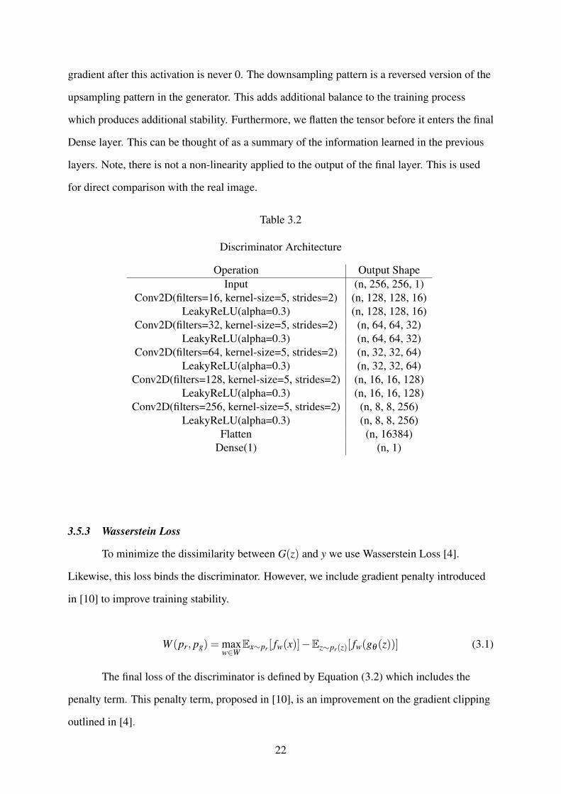
gradient after this activation is never 0. The downsampling pattern is a reversed version of the
upsampling pattern in the generator. This adds additional balance to the training process
which produces additional stability. Furthermore, we flatten the tensor before it enters the final
Dense layer. This can be thought of as a summary of the information learned in the previous
layers. Note, there is not a non-linearity applied to the output of the final layer. This is used
for direct comparison with the real image.
Table 3.2
Discriminator Architecture
Operation Output ShapeInput (n, 256, 256, 1)
Conv2D(filters=16, kernel-size=5, strides=2) (n, 128, 128, 16)LeakyReLU(alpha=0.3) (n, 128, 128, 16)
Conv2D(filters=32, kernel-size=5, strides=2) (n, 64, 64, 32)LeakyReLU(alpha=0.3) (n, 64, 64, 32)
Conv2D(filters=64, kernel-size=5, strides=2) (n, 32, 32, 64)LeakyReLU(alpha=0.3) (n, 32, 32, 64)
Conv2D(filters=128, kernel-size=5, strides=2) (n, 16, 16, 128)LeakyReLU(alpha=0.3) (n, 16, 16, 128)
Conv2D(filters=256, kernel-size=5, strides=2) (n, 8, 8, 256)LeakyReLU(alpha=0.3) (n, 8, 8, 256)
Flatten (n, 16384)Dense(1) (n, 1)
3.5.3 Wasserstein Loss
To minimize the dissimilarity between G(z) and y we use Wasserstein Loss [4].
Likewise, this loss binds the discriminator. However, we include gradient penalty introduced
in [10] to improve training stability.
W (pr, pg) = maxw∈W
Ex∼pr [ fw(x)]−Ez∼pr(z)[ fw(gθ (z))] (3.1)
The final loss of the discriminator is defined by Equation (3.2) which includes the
penalty term. This penalty term, proposed in [10], is an improvement on the gradient clipping
outlined in [4].
22

L = Ex∼ Pg[Dw(x)]− [Dw(x)]+λ (‖∇xDw(x)‖2−1)2 (3.2)
3.5.4 Frequency Domain Loss
In Equation (3.3), φ represents the B-scan frequency transformation outlined in [33]
with some minor modifications. Each A-scan that is contained in the B-scan has a Short Term
Fourier Transform (STFT) [2] with 1024 FFT bins and 16 segment size applied. From these
transforms, we take the max frequency from each A-scan. The max frequencies are then
concatenated back together to form a Frequency B-scan. We do take the transformation a step
further, by converting the Frequency B-scan to gray-scale. This allows for a 1:1 comparison
with time domain B-scans. Furthermore, we are able to use the same number of channels in
the model architecture.
E(x,z)∼P
[∣∣∣∣φ(x)−φ(G(z))∣∣∣∣] (3.3)
3.5.5 Training Algorithm
Algorithm 1 is the process we follow for training the GAN model. This process does
not differ greatly from [10]. However, we do make some modifications. The first modification
is we adopt a faster α for Adam [18]. We found the original learning rate as specified in the
paper to cause slower convergence. We also add 3.3 to line 9. This loss is added directly to the
respective Wasserstein losses. We minimize the weighted sum of all losses for the generator
and discriminator individually. The algorithm begins with samples of real data and latent
variable. For each iteration of the training loop, the discriminator is updated a total of five
times for each generator update. This is specified by the ncritic argument, which is consistent
in naming with the original paper.
23

Algorithm 1 WGAN with gradient penalty.We use default values of λ = 10, ncritic = 5, α = 0.0003Require: The gradient penalty coefficient λ , the number of critic iterations per generator ncritic,the batch size m, Adam hyper-parameter α .Require: initial critic parameters w0, initial generator parameters θ0.
1: while validation loss is still decreasing do2: for t=1,...,ncritic do3: for i=1,...,m do4: Sample B-scan x v Pr, latent variable z v p(z)5: x←− G0(z)6: x←− εx+(1− ε)x7: L(i)←− Dw(x)−Dw(x)+λ (‖∇xDw(x)‖2−1)2
8: L(i)2 ←−
[∣∣∣∣φ(x)−φ(G(z))∣∣∣∣]
9: end for10: w←− Adam(∇w
1m ∑
mi=1 L(i),w,α)
11: end for12: Sample a batch of latent variable {z(i)}m
i=1 v p(z)13: θ ←− Adam(∇w
1m ∑
mi=1−Dw(Gθ (z)),θ ,w,α)
14: end while
3.6 Object Identification Model
We train a separate auxiliary classifier to predict the object in the image. This is a basic
classifier that uses cross entropy to create a separation boundary between classes. The
architecture consists of two convolution layers that lead into a fully connected layer. The
output of the final fully connected layer is activated with softmax to generate a categorical
probability distribution. The loss function 3.4 is traditional categorical cross entropy.
−M
∑c=1
yo,c log(y) (3.4)
We apply this loss to both the Time B-scan and Frequency B-scan to maximize the
probability of a correct class prediction. Figure 3.3 depicts the basic classifier architecture.
The basic classifier has two convolution layers, both activated with Leaky ReLU [32]. We use
this opposed to traditional ReLU to mimic the architecture of the discriminator. In the initial
tests we sought to use the discriminator as the classifier. However, this leads to extreme over
fitting in the discriminator and poor performance for the classification task. Moreover, this
24

also had a negative effect in the adversarial game, with the generator being able to constantly
fool the discriminator. An important note in using a separate classifier is that this simple
architecture can be a stand in for more complex object detection models such as
Faster-RCNN[26] or Mask-RCNN[11]. This was an additional reason for not using the
discriminator as the object detection model. To enable the use of the Time B-scan and
Frequency B-scan, the architecture has a slight modification as depicted in Figure 3.4. The
additional fully connected layer allows us to calculate a separate loss for the Frequency
B-scan which is useful in training.
Table 3.3
Single Classifier Architecture
Operation Output ShapeInput B-scan (n, 256, 256, 1)
Conv2D(filters=2, kernel size=1, strides=2) (n, 128, 128, 2)LeakyReLU(alpha=0.3) (n, 128, 128, 2)
Conv2D(filters=4, kernel size=1, strides=2) (n, 64, 64, 4)LeakyReLU(alpha=0.3) (n, 64, 64, 4)
Flatten (n, 16384)Dense (n, 3)
Table 3.4
Combined Classifier Architecture
Operation Output ShapeInput Time B-scan (n, 256, 256, 1)
Input Frequency B-scan (n, 256, 256, 1)SingleClassifier(Time B-scan) (n, 64, 64, 4)
SingleClassifier(Frequency B-scan) (n, 64, 64, 4)Multiply (n, 64, 64, 4)Flatten (n, 16384)Dense (n, 3)
The auxiliary classifier is trained in three scenarios. The first, data containing only
images from gprMax are adopted. We use this performance as a baseline to compare our other
25

experiments. The second, we use the full gprMax generated dataset with additional GAN
generated images. Finally, we add a concurrent frequency domain optimization function to the
generator, then train the object detection model to identify cylinder material from the b-scan
with the assistance of information from the frequency representation.
26

CHAPTER 4
RESULTS AND DISCUSSION
4.1 Introduction
In the following sections, the results of the experiments along with their significance
are presented and discussed. To begin, the GAN results are presented and discussed.
Furthermore, many generated images are included for the reader to get a qualitative look.
Finally, the object identification performance is displayed and discussed. This is the key area
to identify the validity of the generative models ability to synthesize realistic images that
improve the classification performance.
4.2 Unsupervised GAN Experiments with Real B-scans
In this section, we will be looking at experiments with real B-scan images. These are
unsupervised because we do not have labels for these data. However, it is still possible to
demonstrate that the GAN architecture can produce aesthetically pleasing images from field
collected B-scans. These data were collected by University of Vermont at their GPR test site
and consist of several underground cylinders of various material. An important distinction to
make is that due to the lack of hyperbola variation in the training data, only certain hyperbola
are possible in the generated sets. However, in GPR we actually want to limit the shape
variation of the generated hyperbola. Therefore the focus is on variation in the noise
surrounding the hyperbola. The next section demonstrates that our model is not limited in the
capacity of background variation even with the retention of original hyperbola shape.
4.2.1 Realistic Noise Comparison
Figure 4.1 demonstrates the level of noise variation in two similar B-scans. The
hyperbola is virtually the same, but as one can see the noise surrounding has drastic
27

differences. If we recall in Section 2.2, the noise is indicative of the dielectric properties of the
surround soil. Therefore, a different level of background perturbation allows us to mimic
different soil types that may have not been present in the training set. Resiliency to different
soil types is a prime feature to have in a robust classifier for underground objects and a major
focus of this work. Moreover, as will be demonstrated in Section 4.3, it is possible to
condition the possible locations of the hyperbola if positional variation in the training set is
present. In this case, there will be interpolation between all possible hyperbola positions.
However, this still does not affect the shape or material of the hyperbola.
(a) Generated A (b) Generated B
Figure 4.1
Soil Variance Comparison in Similar B-scans
4.2.2 Sample Diversity
An important discussion of generative results is the diversity of the samples. In Figure
4.2, we can see that our generative model supplies a diverse set of samples. Note that the
hyperbolas do not see much variation, this is the desired behavior. Moreover, one should pay
special attention to how the noise changes between samples. Visually, not a single noise
distribution is identical. In Section 2.7.1, we discussed a paradox when it comes to evaluating
generative models. This paradox is especially important in sample diversity of unsupervised
experiments which we do not have explicit class labels. The argument is that at what point are
we simply memorizing the training distribution and how to define this point. Qualitatively, we
28

see that our generative model does produce visually different images, but saying definitely that
our model is not simply memorizing the training examples is a bit elusive. We do know that
not a single identical image is produced, and that the images are visually realistic. However,
exactly how close the images are to the training set is not quantitatively clear. The next section
discusses the class conditioning results, which is a better approach to identify sample
diversity.
Figure 4.2
Realistic Generated Images
4.3 Supervised GAN Experiments
In this section, we will look at the results of Supervised GAN Experiments. These are
the set of experiments that contain class conditioning. This is only possible with the use of
29

GprMax that allows us to simulate the material of the underground object and retain a
definitive label. This is necessary in the classification task and also a major drawback of
collected B-scans. In the field, B-scans that are collected do not have a ground truth class label
due to the subjective nature of real B-scan evaluation. In this experiment, we can generate
realistic type data that does have a definitive class label. Therefore, we are able to map a set of
image features to the label.
4.3.1 Class Conditioning Examples
Figure 4.3 shows examples of the different classes that were the targets. The GAN
model was able to learn distinct features of each class and then generate images of this type
when given a label. An important note on continuation of this work is that ideally one would
want to be able to combine the Unsupervised with the Supervised to generate a real B-scan
with a known class. This is theoretically possible, however it is beyond the scope of this work.
30

(a) Concrete (b) Metallic
(c) PVC
Figure 4.3
Generated B-scan of Each Class
4.3.2 Sample Diversity
To demonstrate the diversity in samples, the reader is directed to Figure 4.4. As one
can see the diversity compared to the unsupervised experiments, especially in the hyperbola, is
greater. This is due to the ability of being able to control the exact location of the hyperbola.
Therefore, in the simulation through GprMax we can make certain that there is maximum
variability in the training data. Furthermore, we get interpolation between positions of the
hyperbola. This effect is due to defining a range where the hyperbola can occur. Moreover,
with multiple hyperbola positions the model can learn the probable location of where a
hyperbolas can occur which is evident by the high variability of hyperbola location in the
31

generated set. Another important aspect is that even though the hyperbola changes position, it
does not change shape and retains the characteristics of the particular material class. This is of
vital importance because any change in shape or visibility can be interpreted as a different
object than the desired target one.
Figure 4.4
Generated Time B-scans
4.3.3 Frequency Sample Diversity
Figure 4.5 demonstrates the diversity in the generated Frequency B-scans. An
important note is that these are not all of the possible variations, but a small subset for
conciseness. In the frequency domain, we see that the model retains the ability to generate a
wide array of features. Identical to the previous sections, we do not want to see variation in the
hyperbola shape. Again, notice the noise variation, which ranges from very little noise in the
32

background, to almost masking the hyperbola. This level of variation will be important in
classifier evaluation.
Figure 4.5
Generated Frequency B-scans using Figure 2.5
4.4 Object Identification Performance
The following sections are the performance of the proposed classifier in each test
scenario. The main objective is to demonstrate improvement in two places. We would like to
see performance improvement with data augmentation via GAN generated images and further
improvement when combining the time and frequency B-scans.
33

4.4.1 Time Domain
For this set of experiments, we are only using time domain B-scans. These are the
traditional B-scan representations that are present in the field collected examples presented in
Section 4.2 and simulated in first part of Section 4.3. Performance in this area is a key
baseline to realized performance in the subsequent sections.
Table 4.1
Baseline Object Detection Performance
Before AugmentationClass Accuracy Precision Recall F1 N
Concrete 1.00 0.54 1.00 0.70 20Metallic 0.81 1.00 0.82 0.90 11
PVC 0.50 0.67 0.57 0.62 14All 0.77 0.74 0.80 0.75 45
After AugmentationClass Accuracy Precision Recall F1 N
Concrete 1.00 0.88 1.00 0.93 14Metallic 0.91 1.00 0.91 0.95 11
PVC 0.90 0.95 0.90 0.92 20All 0.94 0.94 0.94 0.93 45
From Table 4.1, we present the tabular results of the baseline performance. It is
important to point out that these results are still in the upper half in regards to the performance
metrics. However, as it will be demonstrated, there is still room for improvement. PVC is by
far the worst performing material class. This is due to the lack of reflectivity in PVC cylinders.
In Figure 4.3, it can be seen that PVC is visually, the least prominent hyperbola followed
closely by concrete. From the results, this visibility difference translates to the classifier
performance. Metallic, being the most visually prominent, is easily identified by the detection
model. The lower portion of Table 4.1 shows the performance achieved by training the
classifier with augmented data. Overall, there is a performance increase when adding
augmented training data. Most importantly, this is seen in the weak areas of the classifier. In
the accuracy of PVC there is significant improvement that closes the gap between PVC and
metallic cylinders. This means that when more samples are present in the training data that an
overall increase in classifier performance will be realized.
34

(a) Accuracy (b) Precision
(c) Recall (d) F1
Figure 4.6
Time Results
Figure 4.6 is a visual representation of the performance improvement. The blue bar is
the performance without augmentation and the orange is improvement factor with
augmentation. The total bar height is the final result achieved in each performance metric.
35

Note that for metallic cylinders performance does not have a large increase, but augmentation
improved almost every metric for concrete and PVC cylinders. Next, we will see how the
classifier performs in only the frequency domain.
4.4.2 Frequency Domain
The next section discusses a classifier only trained on frequency B-scans. This
experiment was to determine if the frequency representation leads to better performance in a
particular class.
Table 4.2
Frequency Object Detection Performance
Before AugmentationClass Accuracy Precision Recall F1 N
Concrete 0.21 0.80 0.21 0.33 19Metallic 0.18 1.00 0.62 0.77 16
PVC 0.20 0.75 0.90 0.51 10All 0.20 0.86 0.58 0.54 45
After AugmentationClass Accuracy Precision Recall F1 N
Concrete 0.64 0.83 1.00 0.90 19Metallic 0.36 1.00 0.88 0.93 16
PVC 0.60 1.00 0.60 0.67 10All 0.53 0.94 0.83 0.83 45
Table 4.2 contains the numerical performance results. The classification of PVC
outperformed that of metallic in accuracy when using a frequency B-scan. The significance in
this is that if frequency information is given to the classifier that the weakest class in the
baseline is able to be detected at a better rate than the strongest performing baseline class.
Notice that precision in the frequency domain is high in all of the classes. Recall is an
additional area in which PVC performs well. Although, performance is not quite as good as
the time domain classifier trained with augmented data. Next, let us look at how augmentation
can improve performance in the frequency domain. The bottom half of 4.2 contains the
metrics after augmentation. Overall, there is improvement in all metrics.
36

(a) Accuracy (b) Precision
(c) Recall (d) F1
Figure 4.7
Frequency Results
Figure 4.7 is a visual demonstration of the improvement factor realized by using
augmented data. An important area of improvement is in the Concrete class. Identification of
37

Concrete was greatly improved by augmentation. Again, this is due to the improved detection
ability that comes from using a frequency representation. This is evident when compared to
the Metallic class. This class has the smallest improvement factor, because it was initially the
best performing and also the most visible class. Finally, we will take a look at the performance
when using a combined approach for material classification.
4.4.3 Combined Approach
In the combined approach, we are using both time domain and frequency domain
B-scans. This essentially is doubling the amount of features used for classification. As
reviewed in previous sections, frequency representations allowed improvement for the weak
areas of material classification. A combined approach will yield an improved classifier for all
materials.
Table 4.3
Combined Object Detection Performance
Before AugmentationClass Accuracy Precision Recall F1 N
Concrete 1.00 0.54 1.00 0.70 18Metallic 0.91 1.00 0.93 0.96 14
PVC 0.55 1.00 0.69 0.62 13All 0.82 0.85 0.87 0.76 45
After AugmentationClass Accuracy Precision Recall F1 N
Concrete 1.00 0.88 1.00 0.93 14Metallic 1.00 1.00 1.00 1.00 11
PVC 0.95 1.00 0.90 0.95 20All 0.98 0.96 0.97 0.96 45
Table 4.3, depicts the classification scores achieved before the use of augmented data.
Compared to the baseline, this approach realizes a significant increase in all evaluation
metrics. Notice that PVC is still the worst performer in accuracy. However, it still sees an
improvement from the baseline. This indicates that using a combined approach did improve
the results of a weak class in accuracy. This is also true for the other metrics in relation to
PVC. Concrete did not see an improvement from the baseline when adding features from the
38

frequency domain. This is unusual due to the increased performance in all metrics from the
frequency domain experiments. However, it is important to note that Concrete already
achieved max values in accuracy and precision in the baseline test. Therefore, the
improvement did not occur in precision only. The two other classes, Metallic and PVC, saw
performance improvement in every metric with the combined approach. Thus meaning that a
combined approach is superior to using only time domain or frequency domain features
individually. Now, we will look at the effect augmentation had on the combined classifier
performance.
39

(a) Accuracy (b) Precision
(c) Recall (d) F1
Figure 4.8
Combined Results
Figure 4.8, shows the improvement factor of adding augmented data. The
improvement factor is smallest among all of the experiments. This is due to the already
40
significant performance increase from incorporating frequency domain features. Continuing
the previous trends, PVC is the weakest and also enjoys the most performance improvement
from augmented data.
4.5 Summary
In conclusion, it was demonstrated that GAN could be successfully applied to GPR
data. This is shown in both real and simulated B-scans. In addition, we looked at how the
class conditioning could be applied to GAN to generate labeled training data for a classifier.
With this training data, it was shown that GAN augmentation can improve a classifier.
Furthermore, frequency domain features can be applied in a combined classifier, which
enabled an additional boost in the scoring metrics for the classifier.
41

CHAPTER 5
CONCLUSION
5.1 Final Thoughts
The application of generative models to any domain, has its challenges. As we saw
with applying GAN to GPR, there are some unique challenges to overcome. This thesis is a
first step to further exploration of generative models for GPR. From this work, it was
determined that GAN can successfully be applied to real GPR images. In addition, with the
use of labeled training data, a conditional generative architecture can be applied for data
augmentation. Furthermore, it was shown that a real-time classifier can be trained to detect the
material of underground objects, and that this model can be improved with the incorporation of
frequency domain features in classification. Moreover, With the addition of GAN synthesized
data, we can train a classifier that detects objects with very high classification scores.
5.2 Future Work
Future research opportunities are, for the most part, infinite. However, the following
are some immediate areas where improvement could be made as a continuation of this work.
5.2.1 Sophisticated Object Detection in Real Time
The first major improvement would be the addition of a more complex object detection
model. Due to the desire of real time constraints, a model similar to YOLO-Lite [23] would be
ideal. Figure 5.1, shows some preliminary work in adding YOLO to GPR data. From the
figure, it is evident that more work needs to be done in this area.
42

Figure 5.1
Preliminary Results With YOLO-Lite
This would not be the first work in the field on using sophisticated object detection.
However, to my knowledge, an architecture that is capable of advanced object detection in real
time has not been explored in the GPR space.
5.2.2 Ideal GAN Architecture: gprGAN
Recently, a major realization of the nature of GPR data came to mind. Ground
penetrating radar data is sequential in nature. In review of earlier material, a single B-scan
consists of multiple A-scans. Therefore, it follows that an architecture could exist that
encapsulates the sequential aspect of GPR data. This is most important reason the proposed
model architecture presented in this work, is not named gprGAN or similar, a trait
commonplace in publishing work on adversarial models. A model capable of bearing the
moniker gprGAN, would be able to synthesize sequences of A-scans to assemble a B-scan.
Ideally, this model would be trained on one dimensional wave-forms, and have the ability to
learn temporal dependencies in the segments of B-scans. Therefore, a coherent matrix of
43

A-scans could be generated. The loss function would be a culmination of statistical distances
between each A-scan in the sequence. Furthermore, it would be necessary to encompass the
entire sequence of A-scans. Naturally, this sounds like a hierarchical model architecture and
that could be one way of accomplishing this. In addition, it would be necessary to extending
class conditioning to a multilabel problem. This would have diameter, material, and location
learned independent of each other and the ability to mix these classes in conditional
generation. However, a deeper exploration of this idea is necessary, but it would truly be a
model capable of the title gprGAN.
44

REFERENCES
[1] M. Abadi et al. “TensorFlow: Large-Scale Machine Learning on HeterogeneousDistributed Systems”. In: arXiv e-prints, arXiv:1603.04467 (Mar. 2016),arXiv:1603.04467. arXiv: 1603.04467 [cs.DC].
[2] J. Allen. “Short Term Spectral Analysis, Synthesis, and Modification by DiscreteFourier Transform”. In: IEEE Transactions on Acoustics, Speech, and SignalProcessing 25.3 (June 1977), pp. 235–238. ISSN: 0096-3518. DOI:10.1109/TASSP.1977.1162950.
[3] M. Almaimani et al. “Classifying GPR Images Using Convolutional Neural Networks”.In: EAI, Sept. 2018. DOI: 10.4108/eai.21-6-2018.2276629.
[4] M. Arjovsky, S. Chintala, and L. Bottou. “Wasserstein Generative AdversarialNetworks”. In: Proceedings of the 34th International Conference on Machine Learning.Vol. 70. Proceedings of Machine Learning Research. International Convention Centre,Sydney, Australia: PMLR, Aug. 2017, pp. 214–223. URL:http://proceedings.mlr.press/v70/arjovsky17a.html.
[5] E. L. Denton et al. “Deep Generative Image Models using a Laplacian Pyramid ofAdversarial Networks”. In: CoRR abs/1506.05751 (2015). arXiv: 1506.05751. URL:http://arxiv.org/abs/1506.05751.
[6] R. Ghozzi et al. “Extraction of Geometric Parameters of Underground Tube UsingGPR”. In: 2017 International Conference on Control, Automation and Diagnosis(ICCAD). Jan. 2017, pp. 060–063. DOI: 10.1109/CADIAG.2017.8075631.
[7] C. Gilmore et al. “GPR Target Detection Using a Neural Network Classifier of ImageMoments as Invariant Features”. In: 2004 10th International Symposium on AntennaTechnology and Applied Electromagnetics and URSI Conference. July 2004, pp. 1–4.DOI: 10.1109/ANTEM.2004.7860619.
[8] I. J. Goodfellow et al. “Generative Adversarial Networks”. In: ArXiv e-prints (June2014). arXiv: 1406.2661 [stat.ML].
[9] I. Goodfellow, Y. Bengio, and A. Courville. Deep Learning.http://www.deeplearningbook.org. MIT Press, 2016.
[10] I. Gulrajani et al. “Improved Training of Wasserstein GANs”. In: Advances in NeuralInformation Processing Systems 30. Curran Associates, Inc., 2017, pp. 5767–5777.URL: http://papers.nips.cc/paper/7159-improved-training-of-wasserstein-gans.pdf.
45

[11] K. He et al. “Mask R-CNN”. In: CoRR abs/1703.06870 (2017). arXiv: 1703.06870.URL: http://arxiv.org/abs/1703.06870.
[12] Y. Hong et al. “How Generative Adversarial Nets and its variants Work: An Overviewof GAN”. In: CoRR abs/1711.05914 (2017). arXiv: 1711.05914. URL:http://arxiv.org/abs/1711.05914.
[13] K. Hornik, M. Stinchcombe, and H. White. “Multilayer Feedforward Networks areUniversal Approximators”. In: Neural Networks 2.5 (1989), pp. 359–366. ISSN:0893-6080. DOI: https://doi.org/10.1016/0893-6080(89)90020-8. URL:http://www.sciencedirect.com/science/article/pii/0893608089900208.
[14] J. D. Hunter. “Matplotlib: A 2D Graphics Environment”. In: Computing In Science &Engineering 9.3 (2007), pp. 90–95. DOI: 10.1109/MCSE.2007.55.
[15] Q. Huynh-Thu et al. “Study of Rating Scales for Subjective Quality Assessment ofHigh-Definition Video”. In: IEEE Transactions on Broadcasting 57.1 (Mar. 2011),pp. 1–14. ISSN: 0018-9316. DOI: 10.1109/TBC.2010.2086750.
[16] E. Jones, T. Oliphant, P. Peterson, et al. SciPy: Open Source Scientific Tools for Python.2001. URL: http://www.scipy.org/.
[17] R. M. Joseph and A. Taflove. “FDTD Maxwell’s Equations Models for NonlinearElectrodynamics and Optics”. In: IEEE Transactions on Antennas and Propagation45.3 (Mar. 1997), pp. 364–374. ISSN: 0018-926X. DOI: 10.1109/8.558652.
[18] D. P. Kingma and J. Ba. “Adam: A Method for Stochastic Optimization”. In: CoRRabs/1412.6980 (2014). arXiv: 1412.6980. URL: http://arxiv.org/abs/1412.6980.
[19] J. S. Kobashigawa et al. “Classification of Buried Targets Using Ground PenetratingRadar: Comparison Between Genetic Programming and Neural Networks”. In: IEEEAntennas and Wireless Propagation Letters 10 (2011), pp. 971–974. ISSN: 1536-1225.DOI: 10.1109/LAWP.2011.2167120.
[20] S. Kullback and R. A. Leibler. “On Information and Sufficiency”. In: Ann. Math.Statist. 22.1 (Mar. 1951), pp. 79–86. DOI: 10.1214/aoms/1177729694. URL:https://doi.org/10.1214/aoms/1177729694.
[21] M. Mirza and S. Osindero. “Conditional Generative Adversarial Nets”. In: CoRRabs/1411.1784 (2014). arXiv: 1411.1784. URL: http://arxiv.org/abs/1411.1784.
[22] V. Nair and G. E. Hinton. “Rectified Linear Units Improve Restricted BoltzmannMachines”. In: Proceedings of the 27th International Conference on InternationalConference on Machine Learning. ICML’10. Haifa, Israel: Omnipress, 2010,pp. 807–814. ISBN: 978-1-60558-907-7. URL:http://dl.acm.org/citation.cfm?id=3104322.3104425.
46

[23] J. Pedoeem and R. Huang. “YOLO-LITE: A Real-Time Object Detection AlgorithmOptimized for Non-GPU Computers”. In: CoRR abs/1811.05588 (2018). arXiv:1811.05588. URL: http://arxiv.org/abs/1811.05588.
[24] N. R. Peplinski, F. T. Ulaby, and M. C. Dobson. “Dielectric Properties of Soils in the0.3-1.3-GHz Range”. In: IEEE Transactions on Geoscience and Remote Sensing 33.3(May 1995), pp. 803–807. ISSN: 0196-2892. DOI: 10.1109/36.387598.
[25] M.-T. Pham and S. Lefevre. “Buried Object Detection from B-scan Ground PenetratingRadar Data using Faster-RCNN”. In: CoRR abs/1803.08414 (2018). arXiv:1803.08414. URL: http://arxiv.org/abs/1803.08414.
[26] S. Ren et al. “Faster R-CNN: Towards Real-Time Object Detection with RegionProposal Networks”. In: CoRR abs/1506.01497 (2015). arXiv: 1506.01497. URL:http://arxiv.org/abs/1506.01497.
[27] T. Salimans et al. “Improved Techniques for Training GANs”. In: arXiv e-prints,arXiv:1606.03498 (June 2016), arXiv:1606.03498. arXiv: 1606.03498 [cs.LG].
[28] F. Santambrogio. “Introduction to Optimal Transport Theory”. In: arXiv e-prints,arXiv:1009.3856 (Sept. 2010), arXiv:1009.3856. arXiv: 1009.3856 [math.CA].
[29] N. P. Singh and M. J. Nene. “Buried Object Detection and Analysis of GPR Images:Using Neural Network and Curve Fitting”. In: 2013 Annual International Conferenceon Emerging Research Areas and 2013 International Conference on Microelectronics,Communications and Renewable Energy. June 2013, pp. 1–6. DOI:10.1109/AICERA-ICMiCR.2013.6576024.
[30] C. Warren, A. Giannopoulos, and I. Giannakis. “GprMax: Open Source Software toSimulate Electromagnetic Wave Propagation for Ground Penetrating Radar”. In:Computer Physics Communications 209 (2016), pp. 163–170. ISSN: 0010-4655. DOI:https://doi.org/10.1016/j.cpc.2016.08.020.
[31] A.-M. Wazwaz. “The Tanh and the Sine-cosine Methods for Compact and NoncompactSolutions of the Nonlinear Klein-Gordon Equation”. In: Appl. Math. Comput. 167.2(Aug. 2005), pp. 1179–1195. ISSN: 0096-3003. DOI: 10.1016/j.amc.2004.08.006. URL:http://dx.doi.org/10.1016/j.amc.2004.08.006.
[32] B. Xu et al. “Empirical Evaluation of Rectified Activations in Convolutional Network”.In: CoRR abs/1505.00853 (2015). arXiv: 1505.00853. URL:http://arxiv.org/abs/1505.00853.
[33] W. Zhang et al. “Time-frequency Analysis of Enhanced GPR Detection of RF TaggedBuried Plastic Pipes”. In: NDT & E International 92 (2017), pp. 88–96. ISSN:0963-8695. DOI: https://doi.org/10.1016/j.ndteint.2017.07.013. URL:http://www.sciencedirect.com/science/article/pii/S0963869516302377.
47

[34] Y. Zhang, D. Huston, and T. X. yzhang. “Underground Object Characterization basedon Neural Networks for Ground Penetrating Radar Data”. In: NondestructiveCharacterization and Monitoring of Advanced Materials, Aerospace, and CivilInfrastructure 2016. Vol. 9804. 2016.
48
VITA
After graduating with a Bachelor of Science in Interdisciplinary Studies with a focus on
Biology and Business from East Tennessee State University, Will Rice decided to change
directions and pursue a Masters in Computer Science. In the first year of Masters study, he
landed an internship in network administration at Life Care Centers of America. Within the
first few months, he discovered a passion for machine learning which lead to an internship in
speech and natural language processing at Pylon, ai where he was able to flourish in
applications of machine learning and most importantly, generative models. Will assisted in the
design and deployment of many deep learning models. The most complex being, a state of the
art Text-to-Speech system which is a core component of the app RadioBrain. With a desire to
enhance his technical writing, he decided that an important component to his education would
be the completion of a thesis that applied generative models to a real world application. This
was successfully accomplished with the guidance of Dr. Wu and Dr. Liang in the Networked
Intelligence lab in the University of Tennessee at Chattanooga’s Sim Center. In May 2019, he
graduated with an MSc. in Computer Science.
49
Top Related