


Languages
Pages
Legal


Applying Case Based Decision Theory to the Netflix Competition
Michael Naaman
Abstract
The Netflix competition started out in 2005 as a grassroots competition to improve on the
Cinematch recommendation system by 10% in RMSE with the winner receiving one million
dollars in prize money. Nearly three years later, there was no single algorithm that won the day,
but this paper presents an alternative algorithm that performed better than the Cinematch
algorithm, but fell short of the winning blend of algorithms. We will also show how are approach
can be combined with other algorithms to make further improvements in recommendation
systems.

Introduction
The Netflix project was a competition to help solve an information problem. Netflix is a
company that rents movies on the Internet. Customers make a list of movies that they are
interested in and Netflix mails them those movies as they become available. Then the customer
watches the movies and sends it back to Netflix, but Netflix charges only a membership fee
without any late fees or rental fees. Thus Netflix can only increase its revenue by getting new
members or by getting its old members to upgrade to a more expensive membership. For
example, a customer could upgrade from two movies being sent at a time to three movies at a
time.
They beauty of being an Internet company is that Netflix has a huge centralized
collection of movies that can be distributed cheaply, but that is also the problem: Netflix has so
many movies that the customers are flooded with choices. It was easy for customers to search
for movie they wanted, but there was no knowledgeable rental store clerk to recommend a good
drama like there was in a physical movie rental store.
The solution was to try to make a virtual recommendation system so that people could
find movies that were unknown to them or maybe even a forgotten classic. This way Netflix
could send the customers recommended movies every time they logged on or added a movie to
their rental queue. Hopefully, these recommendations might also be added to the queue and the
customer would get more movies they enjoyed. So Netflix allowed its customers to rate any
movie in the catalogue, including the movies the customer had rented or browsed. Then the
company developed an algorithm called Cinematch that tried to predict which movies the
customer might like based on the ratings of other customers. The idea was to find a movie that
John Doe might like, but hadn't already rented by figuring out which other customers were very

similar to John Doe. Then for any particular movie that John Doe had never rated or rented, the
similar customers could be used as a proxy for John Doe's preferences, thereby allowing Netflix
to make recommendations based on the similar customers' preferences.
As Netflix saw it, the quality of its recommendation system was what would make them
stand apart from future competitors, so they outsourced it to everyone. They developed the
Netflix Prize in which anyone who could beat the Cinematch program by 10% in RMSE, root
mean square error, would win a million dollars and publish the results.
It turned out to be quite difficult to reach that 10% improvement and took almost three
years. There was no single idea that won the day. The winning team, BellKor, was a blend of
algorithms from the most successful teams and there were 107 different estimators used in the
winning algorithm. As Abu-Mostafa (2012) points out, even the winning algorithm was only a
10.06% improvement on the CineMatch algorithm. In fact this bound was so tight that the
second place team, The Ensemble, submitted a solution that tied the BellKor team, but alas it
was submitted 20 minutes too late. While the 10% improvement was chosen rather arbitrarily, it
proved to be a monumentally difficult task.
The setup of the contest was to supply the competitors with three things: the quiz set, the
probe set, and the training set. The training set contains data on the 480189 customers and
17770 movies. The movie titles are given, but for privacy reasons the customer names are not
given. For each customer there is a file that contains all of the ratings that customer has ever
made, except for the ones that have been removed for the quiz set, and the date of that rental.
The quiz set is a randomly chosen subset of the training set with the ratings removed. The quiz
set is where teams make their predictions and send them to Netflix. Netflix computes the RMSE
for the quiz set and sends the results back. Finally, the probe set is another subset of the training
set, but this time the ratings are not removed. The idea of the probe set is that teams could
practice with a similar dataset in order to hone their algorithms.
There were thousands of teams all over the world using all different types of algorithms.
To fix ideas, we present some of the algorithms other teams have used.
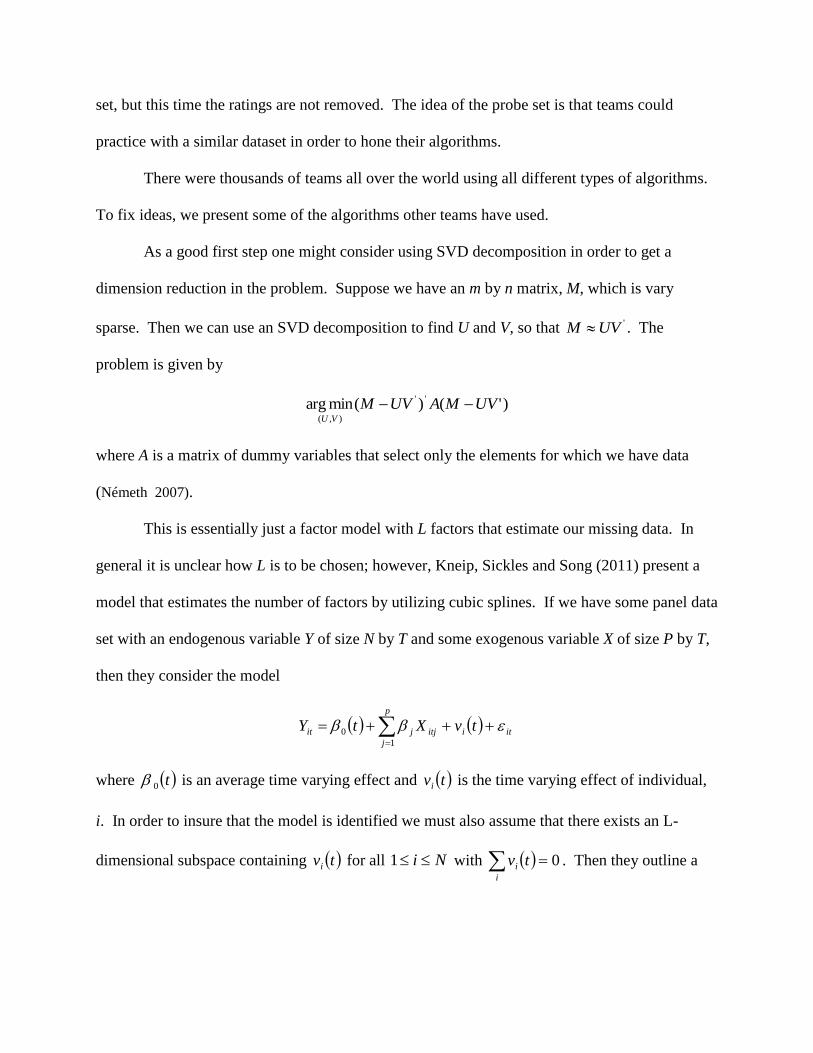
As a good first step one might consider using SVD decomposition in order to get a
dimension reduction in the problem. Suppose we have an m by n matrix, M, which is vary
sparse. Then we can use an SVD decomposition to find U and V, so that 'UVM . The
problem is given by
)'()(minarg ''
),(
UVMAUVMVU
where A is a matrix of dummy variables that select only the elements for which we have data
(Németh 2007).
This is essentially just a factor model with L factors that estimate our missing data. In
general it is unclear how L is to be chosen; however, Kneip, Sickles and Song (2011) present a
model that estimates the number of factors by utilizing cubic splines. If we have some panel data
set with an endogenous variable Y of size N by T and some exogenous variable X of size P by T,
then they consider the model
p
j
itiitjjit tvXtY1
0
where t0 is an average time varying effect and tvi is the time varying effect of individual,
i. In order to insure that the model is identified we must also assume that there exists an L-
dimensional subspace containing tvi for all Ni 1 with i
i tv 0 . Then they outline a

methodology utilizing a spline basis, which is beyond the scope of this paper, to estimate
p ,1 and the time varying effects )(,1 tvtv n by minimizing
i
Tm
i
ti
p
j
itjitjjtit dssvT
tvXXYYT 1
2)(
,
2
1
1
over and all m-times continuously differentiable functions )(,1 tvtv n with
],0[ Tt . There is also a test that can be performed on the size of L. This approach is nice
because it allows not only the factors to be estimated, but also the number of factors to be used.
While the previous model examined methods to estimate time varying effect, we might
also be interested in the spatial relationship of effects. Blazek and Sickles (2010) investigate the
knowledge and spatial spillovers in the efficiency of shipbuilding during World War II.
Suppose we are producing a ship, q, through some manufacturing process, which takes L
units of labor to produce one ship. In many manufacturing settings, there is an element of
learning by doing based on experience, so assume that shipyard, i, in region, j, learns to build
ship, h, according to the equation
hijhij AEL
where A is a constant, hijE is the experience of shipyard i in region j that will be used in the
production of ship h and 0 represents a parameter ensuring that the number of labor units to
produce a single output good is decreasing as experience increases. Unfortunately experience is
not a measurable quantity, so an econometrician might use the total amount of output as a proxy
for experience so that
hT
m
ijm
O
hij qE1
which is the total cumulative output of shipyard i up until
the time that the production of ship h will begin. However, shipyards within any region are
likely to be hiring and firing workers from the same labor pool, which means we should expect
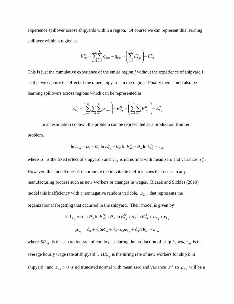
experience spillover across shipyards within a region. Of course we can represent this learning
spillover within a region as
O
hij
I
n
O
hnj
T
m
I
n
ijmnjm
W
hij EEqqEjh j
11 1
This is just the cumulative experience of the entire region j without the experience of shipyard i
so that we capture the effect of the other shipyards in the region. Finally there could also be
learning spillovers across regions which can be represented as
W
hij
J
n
I
O
hno
W
hij
T
m
J
n
I
o
nom
A
hij EEEqEjh j
1 101 1 1
In an estimation context, the problem can be represented as a production frontier
problem.
hij
A
hijA
W
hijW
O
hijOihij vEEEL lnlnlnln
where i is the fixed effect of shipyard i and hijv is iid normal with mean zero and variance 2
V .
However, this model doesn't incorporate the inevitable inefficiencies that occur in any
manufacturing process such as new workers or changes in wages. Blazek and Sickles (2010)
model this inefficiency with a nonnegative random variable, hij , that represents the
organizational forgetting that occurred in the shipyard. Their model is given by
hijhij
A
hijA
W
hijW
O
hijOihij vEEEL lnlnlnln
hijhijhijhijhij HRwageSR 3210
where hijSR is the separation rate of employees during the production of ship h, hijwage is the
average hourly wage rate at shipyard i, hijHR is the hiring rate of new workers for ship h in
shipyard i and 0hij is iid truncated normal with mean zero and variance 2 so hij will be a
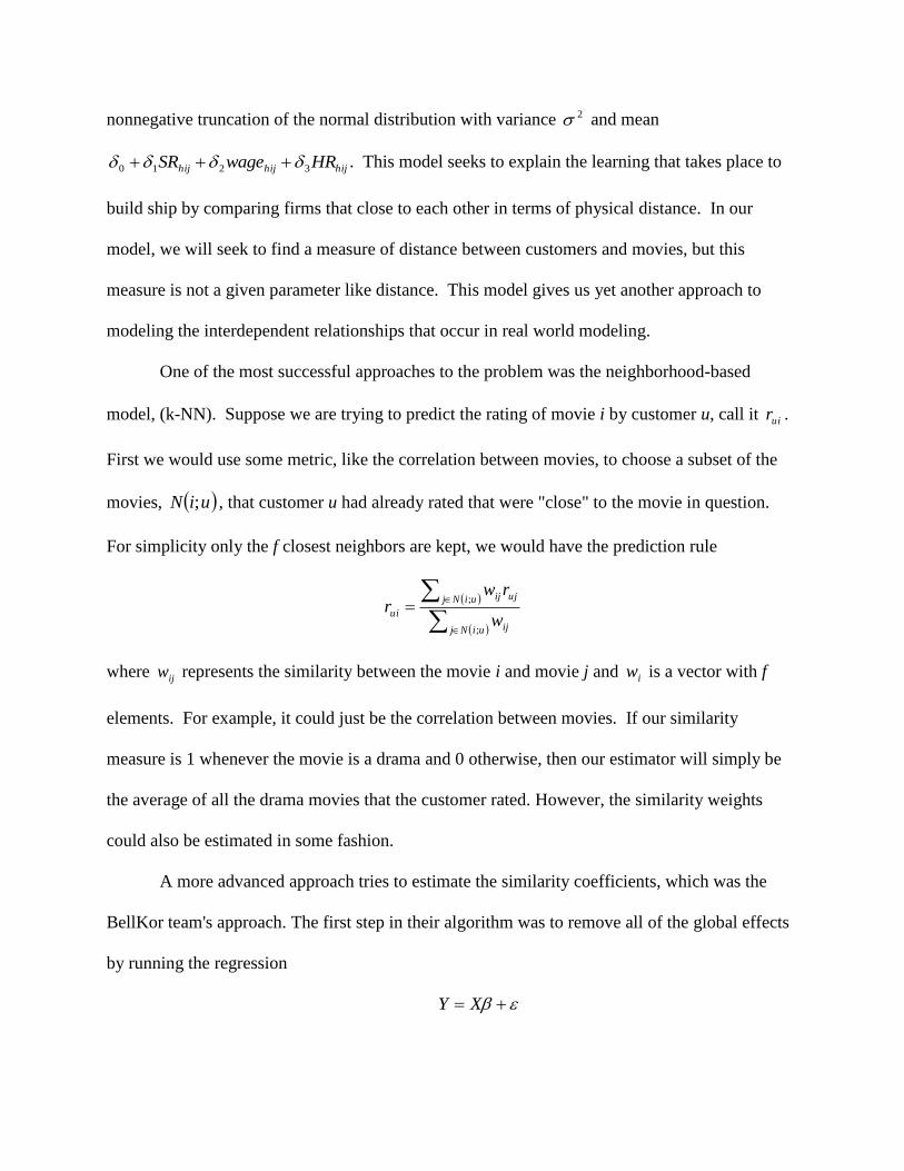
nonnegative truncation of the normal distribution with variance 2 and mean
hijhijhij HRwageSR 3210 . This model seeks to explain the learning that takes place to
build ship by comparing firms that close to each other in terms of physical distance. In our
model, we will seek to find a measure of distance between customers and movies, but this
measure is not a given parameter like distance. This model gives us yet another approach to
modeling the interdependent relationships that occur in real world modeling.
One of the most successful approaches to the problem was the neighborhood-based
model, (k-NN). Suppose we are trying to predict the rating of movie i by customer u, call it uir .
First we would use some metric, like the correlation between movies, to choose a subset of the
movies, uiN ; , that customer u had already rated that were "close" to the movie in question.
For simplicity only the f closest neighbors are kept, we would have the prediction rule
uiNj ij
uiNj ujij
uiw
rwr
;
;
where ijw represents the similarity between the movie i and movie j and iw is a vector with f
elements. For example, it could just be the correlation between movies. If our similarity
measure is 1 whenever the movie is a drama and 0 otherwise, then our estimator will simply be
the average of all the drama movies that the customer rated. However, the similarity weights
could also be estimated in some fashion.
A more advanced approach tries to estimate the similarity coefficients, which was the
BellKor team's approach. The first step in their algorithm was to remove all of the global effects
by running the regression
XY
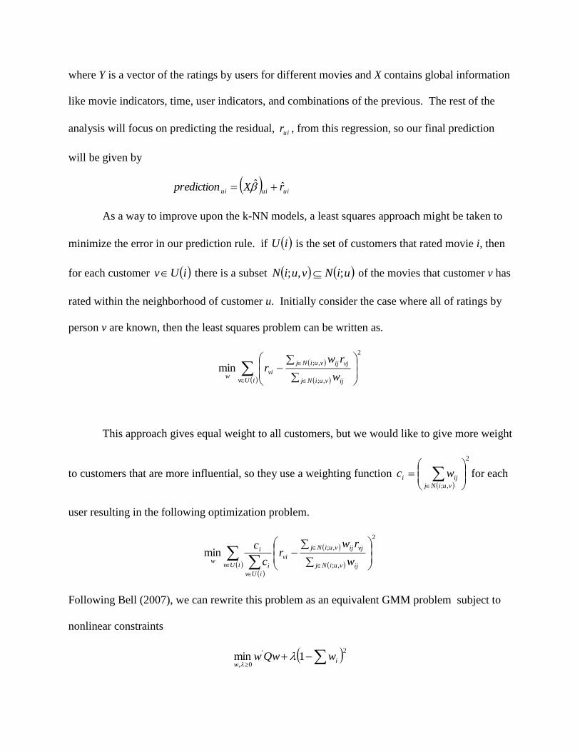
where Y is a vector of the ratings by users for different movies and X contains global information
like movie indicators, time, user indicators, and combinations of the previous. The rest of the
analysis will focus on predicting the residual, uir , from this regression, so our final prediction
will be given by
uiuiui rXprediction ˆˆ
As a way to improve upon the k-NN models, a least squares approach might be taken to
minimize the error in our prediction rule. if iU is the set of customers that rated movie i, then
for each customer iUv there is a subset uiNvuiN ;,; of the movies that customer v has
rated within the neighborhood of customer u. Initially consider the case where all of ratings by
person v are known, then the least squares problem can be written as.
iUv vuiNj ij
vuiNj vjij
viw w
rwr
2
,;
,;min
This approach gives equal weight to all customers, but we would like to give more weight
to customers that are more influential, so they use a weighting function
2
,;
vuiNj
iji wc for each
user resulting in the following optimization problem.
iUv vuiNj ij
vuiNj vjij
vi
iUv
i
i
w w
rwr
c
c2
,;
,;min
Following Bell (2007), we can rewrite this problem as an equivalent GMM problem subject to
nonlinear constraints
2'
0,1min
i
wwQww

where
)(
)(
iUv
jk
iUv
vivkvivjjk
jk
rrrr
Q
and
otherwise
vuiNkjjk
0
,;,1 . However, this approach
ignores some information between customers. If we have some measure, jks , of the similarity
between customers, then we have the simple modification
otherwise
vuiNkjs jk
jk0
,;,
Previously it had been assumed that the ratings were known, but in reality the number of
terms that determine the support for jkQ can vary greatly within the data set, so a shrinkage
factor was used
)(
2)(ˆ
iUv
jk
jk
jk
iUv
vivkvivjjk
jk
Qf
rrrr
Q
where 2f is the number of elements in Q and is a shrinkage parameter. Of course we can
repeat this process by reversing the roles of customers and movies, but it is less effective,
however, the two different results can be combined for further improvements.
Instead of removing the global effects and then estimating the residuals, a refinement can
be made that estimates the global effects and the residuals simultaneously. The basic problem is
given by
0
);();(min
0 ;
2
;
22
,
2
;;
0
0,,
vi
j viRj
ij
viNj
ijj
ivk
viNj
ij
k
viRj
jvvjij
ivvicw
kk
kk
wc
viN
c
viR
rw
r

where viRk ; is the set of the k most similar movies to movie v that have available ratings. This
set takes into account the information of the levels of the ratings, but information is also
available implicitly because the act of rating a movie says provides information that should be
utilized. In order to use this implicit information, viN k ; is the set of k most similar movies to
movie v that are rated by customer i, even if the actual rating is unavailable because it is part of
the quiz set. Previously the term was estimated by a fixed effects approach, but it will be
driven by the data with this approach.
An alternative to k-NN is a latent factor approach. Paterek, A. (2007) approached the
problem by utilizing an augmented SVD factorization model. Under this model, the
optimization problem becomes
iv
vi
j
jivv
T
iivviqp
qppqr, 0
2222
0,,
min
where this sum is taken over all known customer-movie pairs with known ratings. This turned
out to be a very effective approach, but a refinement can be made that includes implicit feedback
as in the previous model.
0
0
;
min
;
222
0
2
;
,
2
0,,,
uiNj
jiv
vi
j
j
k
uiNj
j
vv
iv
v
T
iivviyqp
k
k
yqp
uiN
y
pm
mqr
Here implicit information is being applied to the user portion of the matrix factorization,
which improves RMSE. To get an idea on how these two different algorithms are combines.

This approach still doesn't include the movie-customer interaction term of the SVD model, so the
two approaches can be combined into a single optimization problem given below
0
0
0
;
);();(min
;
222
;
2
;
2
0
2
;
,
2
;;
0
0,,
uiNj
jiv
viRj
ij
viNj
ij
vi
j
j
k
uiNj
j
vv
ivk
viNj
ij
k
viRj
jvvjij
v
T
iivvicw
k
kk
k
kk
yqp
wc
uiN
y
pm
viN
c
viR
rw
mqr
This is just one example of combining two different algorithms into a single approach.
Over the course of the competition, many of the teams collaborated and started to use many
different algorithms until the winning algorithm, which was composed of 3 teams and 107
algorithms. One of the most important lessons learned during the competition was the
importance of using a diverse set of predictors in order to achieve greater accuracy.
Case based utility is based on the idea that memories of our past decisions and the results
of those decisions generate our preferences. That is to say we can represent our preferences as a
linear function of our memories. As discussed in chapter 1, Let A be the set of acts that are
available to the decision maker from some decision problem p. Also let Mr)q,(a,=c be the
triple consisting of the act, a, chosen in a decision problem, p, and the outcome, r, that resulted
from the act. For any given subset of memories, I, preferences can be expressed over acts
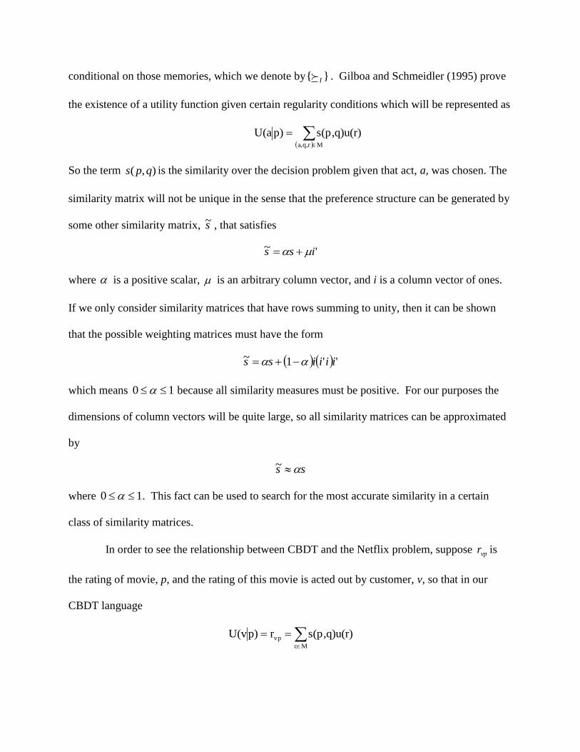
conditional on those memories, which we denote by }{ I . Gilboa and Schmeidler (1995) prove
the existence of a utility function given certain regularity conditions which will be represented as
Mrq,a,
q)u(r)s(p,)pU(a
So the term ),( qps is the similarity over the decision problem given that act, a, was chosen. The
similarity matrix will not be unique in the sense that the preference structure can be generated by
some other similarity matrix, s~ , that satisfies
'~ iss
where is a positive scalar, is an arbitrary column vector, and i is a column vector of ones.
If we only consider similarity matrices that have rows summing to unity, then it can be shown
that the possible weighting matrices must have the form
''1~ iiiiss
which means 10 because all similarity measures must be positive. For our purposes the
dimensions of column vectors will be quite large, so all similarity matrices can be approximated
by
ss ~
where 10 . This fact can be used to search for the most accurate similarity in a certain
class of similarity matrices.
In order to see the relationship between CBDT and the Netflix problem, suppose vpr is
the rating of movie, p, and the rating of this movie is acted out by customer, v, so that in our
CBDT language
Mc
vp q)u(r)s(p,r)pU(v
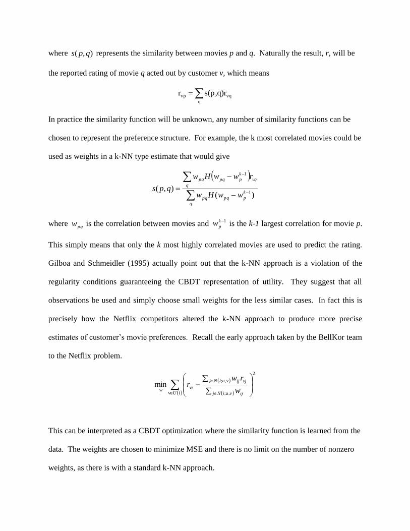
where ),( qps represents the similarity between movies p and q. Naturally the result, r, will be
the reported rating of movie q acted out by customer v, which means
q
vqvp q)rs(p,r
In practice the similarity function will be unknown, any number of similarity functions can be
chosen to represent the preference structure. For example, the k most correlated movies could be
used as weights in a k-NN type estimate that would give
q
k
ppqpq
q
vq
k
ppqpq
wwHw
rwwHw
qps)(
),(1
1
where pqw is the correlation between movies and 1k
pw is the k-1 largest correlation for movie p.
This simply means that only the k most highly correlated movies are used to predict the rating.
Gilboa and Schmeidler (1995) actually point out that the k-NN approach is a violation of the
regularity conditions guaranteeing the CBDT representation of utility. They suggest that all
observations be used and simply choose small weights for the less similar cases. In fact this is
precisely how the Netflix competitors altered the k-NN approach to produce more precise
estimates of customer’s movie preferences. Recall the early approach taken by the BellKor team
to the Netflix problem.
iUv vuiNj ij
vuiNj vjij
viw w
rwr
2
,;
,;min
This can be interpreted as a CBDT optimization where the similarity function is learned from the
data. The weights are chosen to minimize MSE and there is no limit on the number of nonzero
weights, as there is with a standard k-NN approach.

But we may also have a situation where there is similarity between act decision problem
pairs. For example, if our set of acts consists of buying or selling a stock and our set of decision
problems consists of buying the stock when the price is high or low, then we may have a
situation where "buying the stock when the price is low" is more similar to "selling the stock
when the price is high" than "selling the stock when the price is low". Gilboa and Schmeidler
(1997) provide axioms that allow a generalization that includes similarity over the pair of
decision problems and acts by
Mrb,q,
b))u(r)(q,a),w((p,U(a)
This generalization allows for cases and acts to be separated. There are many possibilities, but
Gilboa and Schmeidler (1997) provide a multiplicative approach that satisfies the necessary
axioms. It was presented as
bawqpwbqapw ap ,,,,,
Since the weights are positive, the logarithm or both sides can be taken to derive an additively
separable similarity function given by
bawqpwbqapw ap ,,,,,
This is the similarity function that will be used in our model. As before the utility of any result is
simply the reported ratings of a movie, so
Mqb,
bqapap rb)(a,wq)(p,wr
where apr is the rating provided by customer, a, for movie, p. Recall that the movie represents
the decision problem and the customer represents the act of providing a rating. This weighting
function would have been difficult to implement in practice, so a first order approximation was
used.

b
bpa
q
aqpap b)r(a,wq)r(p,wr
This weighting function keeps only the most informative movie ratings, which are presumably
the ratings made by customer, a, for other similar movies. Similarly the ratings of movie, p, are
weighted by the most similar customers. By assumption 1),( xxw , this fact can used to rewrite
the multiplicatively separable weighting function can be written as
paM/,
bqap
M,
bpa
M,
aqp
Mqb,
bqapap b)r(a,wqp,wb)r(a,wq)r(p,wb)r(a,q)w(p,wrqbpbqa
If the third term is drop, the equivalence can be seen, but a generalization of our model that will
incorporate this functional form will be given later.
b
bpa2
q
aqp1ap b)r(a,wq)r(p,wr
As discussed previously, we are interested in the class of weighting matrices that have rows
summing to unity. As previously demonstrated the weighting matrices will not be unique, but all
of the qualifying matrices can be represented with the functional form above as long as the
restriction 10 21 is imposed. Finally our CBDT based model will have the functional
form
b
bpa
q
aqpap b)r(a,w1q)r(p,wr
with 10 . The details of how such a model can be implemented to predict movie ratings in
the Netflix competition will be discussed below.
Model
This model began as a class project at Rice University. Naaman, Dingh, and Taylor
(2012) used this class project as a springboard to develop a full-scale algorithm for the Netflix

competition. Most of the algorithms focused on using only the information between movies
because there were so many more customers than users and each movie has much more data than
each customer, which is clearly more effective than just using information between customers.
We wanted to directly incorporate this symmetry into our algorithm instead of trying to mash
two different results together. What set our algorithm apart is that it tries to combine the two
sides sort of like digging a tunnel from both sides of the river instead of just one side. However,
the trick was to make sure the tunnel met in the middle.
In calculus one can represent a function at any given point by using the first derivative of
the function evaluated at some other point suitably close. This concept guided are thinking in
that we could take an expansion of the customer's preferences around a particular customer-
movie pair by choosing a small neighborhood of customers and movies that were in some sense
"close" to that customer-movie pair. This seemed to point us in the direction of spatial
regression and case based utility.
Suppose that we have an 1N vector of endogenous variables y and that there exists
some linear expansion of iy in terms of the other endogenous variables so that we can write
i
j
jiji ywy with 0iE
In the context of spatial regression, we interpret the weights as being a representation of a
point on a map using other landmarks on that map. So it seems reasonable to assume that this is a
convex representation, 0W with j
ijw 1 for all i. These weights might be the result of some
other estimation procedure, which is not pursued in this model. Previously examples were given
where some sort of weighted least squares subject to constraints estimated the weights.
Switching to matrix notation, we can write
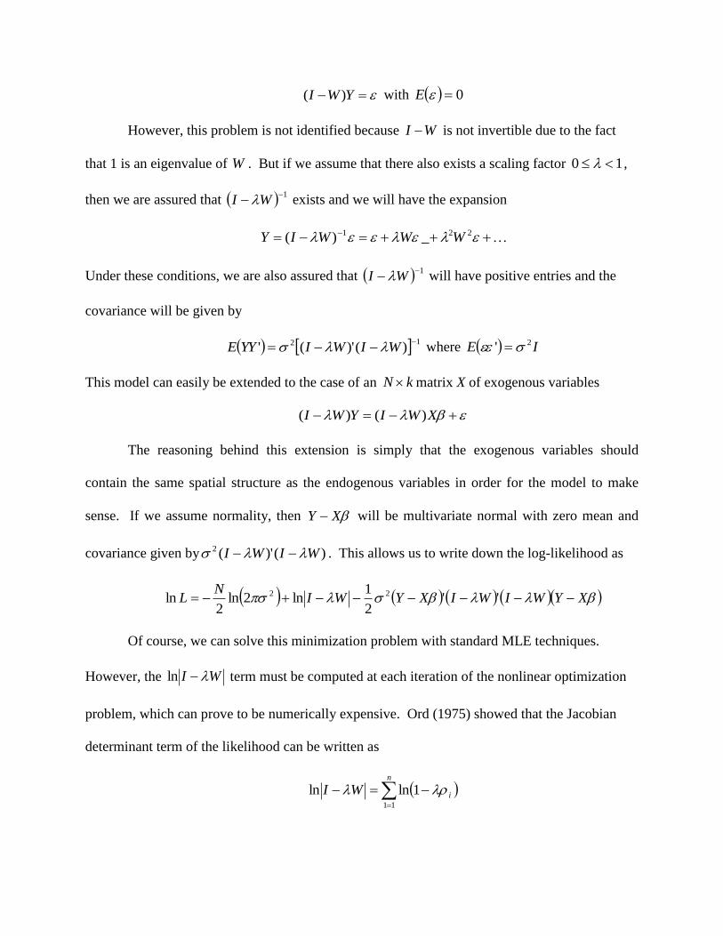
YWI )( with 0E
However, this problem is not identified because WI is not invertible due to the fact
that 1 is an eigenvalue of W . But if we assume that there also exists a scaling factor 10 ,
then we are assured that 1 WI exists and we will have the expansion
221 _)( WWWIY
Under these conditions, we are also assured that 1 WI will have positive entries and the
covariance will be given by
12 )()'('
WIWIYYE where IE 2'
This model can easily be extended to the case of an kN matrix X of exogenous variables
XWIYWI )()(
The reasoning behind this extension is simply that the exogenous variables should
contain the same spatial structure as the endogenous variables in order for the model to make
sense. If we assume normality, then XY will be multivariate normal with zero mean and
covariance given by )()'(2 WIWI . This allows us to write down the log-likelihood as
XYWIWIXYWIN
L ''2
1ln2ln
2ln 22
Of course, we can solve this minimization problem with standard MLE techniques.
However, the WI ln term must be computed at each iteration of the nonlinear optimization
problem, which can prove to be numerically expensive. Ord (1975) showed that the Jacobian
determinant term of the likelihood can be written as
n
iWI11
1lnln

where nii 1, is the set of eigenvalues of the spatial weighting matrix. If we appeal to the
Schur decomposition of a matrix, in general W will not be symmetric, which allows us to write
TQSQW where S is an upper triangular matrix with the eigenvalues of W on the diagonal of S
and Q is an orthogonal matrix.
SIQSIQQSIQWI TT lnlnlnln
The result follows when we realize that SI is an upper triangular matrix with a diagonal
entry iiiS 1 , so the result follows and we have much faster computation. However,
Anselin and Hudak (1992) do find evidence for numerical instability for eigenvalues in matrices
with more than 1000 entries, but for our purposes all of our weighting matrices will not be so
large. This basic model can be extended in many different directions, which are beyond the
scope of this paper, but details can be found in Anselin (1988a).
This approach made sense to us because we felt that correlations could be used as a
measure of distance between customers and movies. If we had some meaningful weighting
matrices that represented the "distance" between movies and customers, then we could apply
some spatial regression techniques to reduce RMSE. However, we couldn't find anything in the
literature that matched up with our needs, which meant our approach was ad hoc and the result of
trial and error.
The first step was to take correlations between movies over the customers that had rated
both movies and take correlations between customers over the movies they had in common.
However, this does not give a good measure of similarity because two customers may only have
one movie in common which tells us little about how similar their preferences are, so the
correlations are weighted based on the number of matches two customers or movies had. So if
customer u has rated p number of movies and customer v has rated q of the movies that customer

u has rated, then the weight for the correlation would simply be sq
q
where s is a scaling factor
that could be p or just a parameter. However if the scaling parameter depends on p, then the
weighted correlation matrix will be asymmetric because the weight for the correlation between
customer u and customer v would still be given by sq
q
, but the scaling parameter would
depend on how many movies customer v has rated. We decided to leave s as a global scaling
parameter so that when z is large the weight will be close to unity and when z is small the weight
will scale the correlation down to zero. It made sense that if two customers had rated a large
number of movies, but they only had a couple movies in common, then they were probably not
very similar and the high correlations were due to the small sample size.
The next global step of our model was the same as most of the other competitors and that
was to get rid of the fixed effects. Let uir be the rating that customer u gave to movie i with the
convention that ur is the average rating of customer u over all the movies that customer u has
rated; and ir is the average rating of movie i over all the customers that have rated movie i; and
r is the grand mean which is the average rating over all customers and all movies. This leaves
us with the residuals given by
rrrry iuuiui
We also tried a random effects model, but that did not perform as well as the fixed effects
approach in terms of out of sample RMSE. Some other panel techniques were also applied, but
they provided no improvement in out of sample RMSE. But the rest of our model will be
working with the residuals of the fixed effects model.
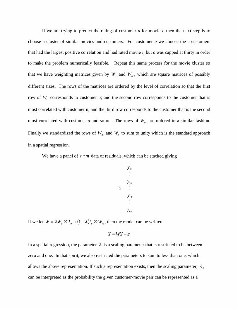
If we are trying to predict the rating of customer u for movie i, then the next step is to
choose a cluster of similar movies and customers. For customer u we choose the c customers
that had the largest positive correlation and had rated movie i, but c was capped at thirty in order
to make the problem numerically feasible. Repeat this same process for the movie cluster so
that we have weighting matrices given by cW and mW , which are square matrices of possibly
different sizes. The rows of the matrices are ordered by the level of correlation so that the first
row of cW corresponds to customer u; and the second row corresponds to the customer that is
most correlated with customer u; and the third row corresponds to the customer that is the second
most correlated with customer u and so on. The rows of mW are ordered in a similar fashion.
Finally we standardized the rows of mW and cW to sum to unity which is the standard approach
in a spatial regression.
We have a panel of mc* data of residuals, which can be stacked giving
cm
c
m
y
y
y
y
Y
1
1
11
If we let mcmc WIIWW 1 , then the model can be written
In a spatial regression, the parameter is a scaling parameter that is restricted to be between
zero and one. In that spirit, we also restricted the parameters to sum to less than one, which
allows the above representation. If such a representation exists, then the scaling parameter, ,
can be interpreted as the probability the given customer-movie pair can be represented as a
WYY

weighted sum of the most similar users and 1 is the probability that the customer-movie pair
is represented as a weighted sum of the most similar movies.
Finally we are ready to minimize the log likelihood,
YWIWIYWIL cmcmcm ''2
1ln
where mcmc WIIWW 1 . In order to improve the speed of this nonlinear
optimization problem, we can again appeal to the Schur decomposition of a matrix. Let
'PPTW cc and 'QQTW mm where P and Q are orthogonal matrices with cT and mT being
upper triangular matrices with the eigenvalues of cW and mW on the diagonals, respectively.
This allows the WI cm ln term on the optimization problem to be rewritten as
c
i
m
j
jimcmcmc
mcmcmccm
TIITII
QPTIITIIQPWI
1 1
11ln1ln
''1lnln
where cii 1, is the set of eigenvalues for cW and mjj 1, is the set of eigenvalues
for mW and the last equality follows from the properties of upper triangular matrices. This
allows for a much quicker numerical computation of the optimization problem.
Once we have our estimator, ̂ in hand, then our prediction for the rating that customer u
will give to movie i is given by 1)ˆ( YWrrr iu and we repeat this process for the next
customer-movie pair. We can extend this model by using the rest of the 1* mc predictions to
impute the missing data. When we move on to the next customer-movie pair, there might be
some overlap in the predicted values of missing data, but we can simply average the different
predictions of the same missing data point. Then we can repeat the whole process using our
averaged predictions for the missing data.

Estimation
The algorithm that we used in the Netflix competition begins with forming the fixed
effects predictor and residual given by
uiuiui
iuui
rry
rrrr
ˆ
ˆ
In general any prediction rule can be used, but the main focus of this approach is to
estimate the residual of the predictor.
The next step in the preprocessing is done by finding the weighting matrix, mW , for the
movie effect. Our weighting matrix is computed by shrinking the Pearson correlation, which
means an element of the movie weighting matrix will be given by
where ijq is the number of common customers for movie i and j. On the right hand side, we
have the Pearson correlation over all of the common customers for movie i and j. On the left, we
have our shrinkage factor, which will be 1 whenever 480189ijq .
This means there will be very little shrinkage for a large number of common customers.
Conversely the weight will be essentially 0 whenever there are few common customers to
support the correlation as a measure of similarity. In a similar fashion, the customer weighting
matrix is calculated as
2.
2
.
..
480189
2
k
iki
k
iki
jkj
k
iki
ij
ij
ijm
rrrr
rrrr
q
qW
2.
2
.
..
17770
2
k
jjk
k
iik
jjk
k
iik
ij
ij
ijc
rrrr
rrrr
p
pW

Once these matrices are formed, the last step of the preprocessing is to find the eigenvalues of
the weighting matrices so that the log-likelihood can be written as
YWIWIY cmcm
c
i
m
j
ji
''2
111ln
1 1
From this point can be estimated be a simple line search. Since we are only interested in
prediction, the asymptotic distribution of our estimator was not worked out, but bootstrapping
the standard errors is feasible, but it was not computationally feasible for our large data set.
Once the estimate is in hand, the prediction for the quiz set can be made for the rating of
customer c for movie m.
1.... )ˆ( YWrrrr mc
pred
cm
There will now be cm-1 other predictions which can be used to impute the missing data, so this
predicted rating will replace any missing data. If there is already a prediction from some other
regression then the predictions will be averaged. The number of predictions that have been made
will be saved so that the averaging can always be done over all of the predictions that have been
made for any missing data point. Of course if the data is not missing, then there is no need to
predict it. This whole procedure is then repeated creating a new predicted rating until we
achieve convergence in RMSE over the probe set. After convergence is reached, all of the
predictions can be submitted for the quiz set.
Results
In order to get an idea about the relationship between the movie and user effects, we
iteratively estimated the RMSE of the different fixed effects. First we calculated the RMSE just
using the overall mean as our predictor; then we added the movie effect to our estimator; and

finally, we estimated the RMSE over the full fixed effects model consisting of customer and
movie effects.
Predictor RMSE Improvement
Overall mean 1.130 NA
Movie mean and overall mean 1.053 0.077
Customer mean, movie mean, and overall mean 0.984 0.069
The main thing to notice about the table above is that adding the movie effect produces a
larger improvement than adding the customer effect to our predictor. Since there are many more
customers than movies, it stands to reason that the movie mean is a more robust predictor than
the user mean because on average there are many more customer ratings for any given movie
than movie ratings for any given user due to the discrepancy between the number of movies and
customers.
We wanted to know the effectiveness of the different parts of our model running a linear
regression over our actual RMSE that came from running our model over the entire probe.
9
1̀i
jijij zRMSE
Independent variable Estimate
Grand mean
00100.0
00010.

Movie mean
00102.0
11608.
User mean
00107.0
0.04138
Lambda
00113.0
0.02369-
Number of ratings in the mc* data set
00118.0
0.08695
Average of the first row of mW
00194.0
0.13912
Average of the first row of cW
00154.0
0.03404 -
Average of all of mW except for the first row 00193.0
0.10803
Average of all of cW except for the first row
00147.0
0.03275
The user mean was not nearly as effective as the movie mean in explaining a small
decrease in RMSE of the model and the grand mean was less effective than both the movie mean
and user mean. This falls in line with the experiences of the other competitors. In fact, most of
the competitors used a movie centric approach which exploited the robustness of the between
movie effects. The next thing to notice is that the spatial weight, lambda, is negatively correlated
with RMSE, so there is strong evidence supporting a spatial approach. As expected the number
of ratings in the data set is also negatively correlated with RMSE, which simply indicates that the
model improves as our data set fills up with actual ratings.

In our model, the single most effective factor was the average of the first row of mW
which is the average weight given to the most similar movies that have been rated by the
customer in question. As we have more highly correlated movies, the average of the first row of
mW increases which leads to a decrease in RMSE in terms of conditional expectation. As we
saw with the customer mean and movie mean, the movie effect is more relevant than the
customer effect, but the model is improved by combing both effects.
It seems counterintuitive that the average entry of cW and mW , excluding the first row of
both matrices, is positively correlated with RMSE. However, this is really a measure of the
similarity between the movies and customers that we are using as a basis to make out estimate
for any given customer-movie pair. In essence, there is some overlap in our neighborhood of
customers and movies. Ideally we would have a set of movies or customers that is very similar
to the rating we are trying to predict, but the set of movies or customers themselves are not very
similar to each other.
The final RMSE for our model over the probe set is given in the table below with some
naïve models as well.
Predictor RMSE Improvement on Cinematch
Overall mean 1.130 -17%
Movie mean and overall
mean
1.053 -15%
Customer mean, movie
mean, and overall mean
0.984 -2%
Cinematch 0.965 0%

Spatial Model (Probe Set) 0.93 3.76%
Spatial Model (Quiz Set) 0.88 8.8%
Winning Algorithm 0.865 10.006%
This is very close to the 10% improvement that we would need to win the Netflix
competition; however, this result is for the probe set which was for practice. When the algorithm
was applied to the Quiz set, the RMSE was 0.92 which was a 4.7% improvement on the
Cinematch algorithm which was well short of the 10% improvement needed to win. Despite our
best efforts, we were never able to explain the discrepancy in accuracy between the two data sets.
Conclusions
In the Netflix competition, we found significant improvements in RMSE by using a
spatial model approach that incorporates the interrelationship between movies and customers.
One drawback of this approach is its computationally difficulty, but the computational burden
can still be handled by most data sets that are encountered in the field and by a judicious choice
of the maximum size of the neighborhood used to make predictions.
There are also future extensions to this model by using more advanced weighting
matrices. One possible future improvement of this model would to use a more complicated
weighting matrix. Recall that the multiplicatively separable model can be written in SBDT form
as
paM/,
bqap
M,
bpa
M,
aqpap b)r(a,wqp,wb)r(a,wq)r(p,wrqbpbqa
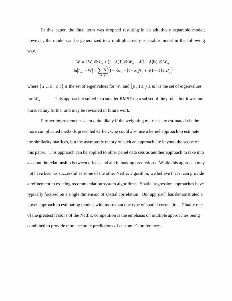
In this paper, the final term was dropped resulting in an additively separable model;
however, the model can be generalized to a multiplicatively separable model in the following
way.
c
i
m
j
jijicm
mcmcmc
WI
WWWIIWW
1 1
111ln
1)1(
where cii 1, is the set of eigenvalues for cW and mjj 1, is the set of eigenvalues
for mW . This approach resulted in a smaller RMSE on a subset of the probe, but it was not
pursued any further and may be revisited in future work.
Further improvements seem quite likely if the weighting matrices are estimated via the
more complicated methods presented earlier. One could also use a kernel approach to estimate
the similarity matrices, but the asymptotic theory of such an approach are beyond the scope of
this paper. This approach can be applied to other panel data sets as another approach to take into
account the relationship between effects and aid in making predictions. While this approach may
not have been as successful as some of the other Netflix algorithm, we believe that it can provide
a refinement to existing recommendation system algorithms. Spatial regression approaches have
typically focused on a single dimension of spatial correlation. Our approach has demonstrated a
novel approach to estimating models with more than one type of spatial correlation. Finally one
of the greatest lessons of the Netflix competition is the emphasis on multiple approaches being
combined to provide more accurate predictions of customer's preferences.

REFERENCES
1. Anselin, L. (1988a). Spatial Econometrics: Methods and Models. Kluwer Academic,
Dordrecht.
2. Anselin, L. (1988b). Lagrange multiplier test diagnostics for spatial dependence and
spatial heterogeneity. Geographical Analysis 20, 1–17.
3. Anselin, L. (1992). Space and applied econometrics. Special Issue, Regional Science and
Urban Economics 22.
4. Anselin, L. and A. Bera (1998). Spatial dependence in linear regression models with an
introduction to spatial econometrics. In: A. Ullah and D. E. A. Giles, Eds., Handbook of
Applied Economic Statistics, pp. 237–289. New York: Marcel Dekker.
5. Anselin, L. and S. Hudak (1992). Spatial econometrics in practice, a review of software
options Regional Science and Urban Economics 22, 509–536.
6. Aten, B. (1996). Evidence of spatial autocorrelation in international prices. Review of
Income and Wealth 42, 149–63.
7. Baltagi, B. and Dong Li (1999). Prediction in the panel data model with spatial
correlation. In L. Anselin and R. Florax (Eds.), Advances in Spatial Econometrics.
Heidelberg: Springer-Verlag.
8. Bell, R., and Y. Koren (2007). Scalable Collaborative Filtering with Jointly Derived
Neighborhood Interpolation Weights. IEEE International Conference on Data Mining
(ICDM'07), IEEE.
9. Bell, R., and Y. Koren (2007). Improved Neighborhood-based Collaborative filtering.
KDD-Cup and Workshop, ACM press.

10. Bell, R., and Y. Koren, and C. Volinsky (2007). The BellKor solution to the Netflix
Prize. http://www.netflixprize.com/assets/ProgressPrize2007_KorBell.pdf.
11. Gilboa I. and D. Schmeidler (1995). Case-based decision theory, Quart. J. Econ. 110,
605–639.
12. Gilboa, I. and D. Schmeidler (1997). Act-similarity in case-based decision theory, Econ.
Theory 9, 47–61.
13. Gilboa, I. and D. Schmeidler (2001). A Theory of Case-Based Decision, Cambridge
Univ. Press, Cambridge, UK.
14. Kneip, A., R.C. Sickles, and W. Song (2011). A New Panel Data Treatment for
Heterogeneity in Time Trends. Econometric Theory.
15. Konstan, J., G. Karypis, J. Riedl, and B. Sarwar (2001). Item-based Collaborative
Filtering Recommendation Algorithms. Proc. 10th International Conference on the
World Wide Web, pp.285-295.
16. Konstan, J., G. Karypis, J. Riedl, and B. Sarwar (2000). Application of Dimensionality
Reduction in Recommender System – A Case Study. WEBKDD’2000.
17. Koren, Y. (2008). Factorization Meets the Neighborhood: a Multifaceted Collaborative
Filtering Model. Proc. 14th ACM Int. Conference on Knowledge Discovery and Data
Mining (KDD'08), ACM press.
18. Koren, Y. Factor in the Neighbors: Scalable and Accurate Collaborative Filtering.
http://public.research.att.com/~volinsky/netflix/factorizedNeighborhood.pdf, submitted.
19. Linden, G., B. Smith and J. York (2003). Amazon.com Recommendations: Item-to-item
Collaborative Filtering, IEEE Internet Computing 7, 76–80.

20. Leroux, J., J.A. Rizzo, and R.C. Sickles (2010). The Role of Self-Reporting Bias in
Health, Mental Health and Labor Force Participation: a Descriptive Analysis. Journal of
Empirical Economics.
21. MaCurdy, Thomas (1983). A Simple Scheme for Estimating an Intertemporal Model of
Labor Supply and Consumption in the Presence of Taxes and Uncertainty. International
Economic Review, 24:2, 265-289.
22. Naaman, M., Trang Dinh, and Jonathon Taylor (2008). Netflix Group Project.
manuscript, Rice University.
23. Németh, B., Gábor Takács, István Pilászy, and Domonkos Tikk (2007). Major
components of the gravity recommendation system. ACM SIGKDD Explorations
Newsletter 9: 80.
24. Németh, B., Gábor Takács, István Pilászy, and Domonkos Tikk (2007). "On the
Gravity Recommendation System" (PDF), Proc. KDD Cup Workshop at SIGKDD, San
Jose, California, pp. 22–30, http://www.cs.uic.edu/~liub/KDD-cup-
2007/proceedings/gravity-Tikk.pdf.
25. Ord, J.K. (1975). Estimation methods for models of spatial interaction. Journal of the
American Statistical Association 70, 120–126.
26. Pencavel, John (1986), “Labor Supply of Men: A Survey,” in O. Ashenfelter and R.
Layard (eds.), Handbook of Labor Economics, Vol. 1, North-Holland, Amsterdam, pp. 3-
102.
27. Paterek, A. (2007). Improving Regularized Singular Value Decomposition for
Collaborative Filtering. KDD-Cup and Workshop, ACM press.
28. Prescott, E. (2004). Why Do Americans Work So Much More than Europeans?.
Quarterly Review of the Federal Reserve Bank of Minneapolis, pp. 2-13.
29. Prescott, E. (2006). Nobel Lecture: The Transformation of Macroeconomic Policy and
Research. Journal of Political Economy 114, pp. 203-235.
30. Ragan, K. (2005). Taxes, Transfers and Time Use: Fiscal Policy in a Household
Production Model. manuscript, University of Chicago.
31. Riedl, J. (2006). ClustKNN: a highly scalable hybrid model-& memory-based CF
algorithm. In Proc. of WebKDD'06: KDD Workshop on Web Mining and Web Usage
Analysis, at 12th ACM SIGKDD Int. Conf. on Knowledge Discovery and Data Mining,
Philadelphia, PA, USA.
32. Rogerson, R. (2006). Understanding Differences in Hours Worked. Review of Economic
Dynamics 9, pp. 365-409.
33. Rogerson, R. (2007). Taxes and Market Work: Is Scandinavia an Outlier?. Economic
Theory 32, pp. 59-85.
34. Rogerson, R. (2008). Structural Transformation and the Deterioration of European Labor
Market Outcomes. Journal of Political Economy 116, pp. 235-259.
35. Rogerson, R., and Johanna Wallenius (2008). Micro and Macro Elasticities in a Life
Cycle Model with Taxes. NBER Working Papers 13017, National Bureau of Economic
Research, Inc.
36. Rogerson, R. (2009). Market Work, Home Work, and Taxes: A Cross-Country Analysis.
Review of International Economics, Blackwell Publishing, vol. 17(3), pages 588-601.
37. Roweis, S. (1997). EM Algorithms for PCA and SPCA. Advances in Neural Information
Processing Systems 10, pp. 626–632.
38. Rupert, P., Richard Rogerson, and Randall Wright (1995). Estimating Substitution
Elasticities in Household Production Models. Economic Theory 6, pp. 179-193.
39. Tibshirani, R. (1996) Regression Shrinkage and Selection via the Lasso. Journal of the
Royal Statistical Society B 58.
40. Wang, J., A. P. de Vries and M. J. T. Reinders (2006). Unifying User-based and Item-
based Collaborative Filtering Approaches by Similarity Fusion. Proc. 29th ACM SIGIR
Conference on Information Retrieval, pp. 501–508.
Top Related