


Languages
Pages
Legal

AmJ
TAa
b
c
d
e
a
ARRAA
KLPMNB
1
tb
N7
h1
Applied Soft Computing 56 (2017) 317–330
Contents lists available at ScienceDirect
Applied Soft Computing
j ourna l h o mepage: www.elsev ier .com/ locate /asoc
neural network-based local rainfall prediction system usingeteorological data on the Internet: A case study using data from the
apan Meteorological Agency
omoaki Kashiwao a,b,∗, Koichi Nakayama a, Shin Ando c, Kenji Ikeda d, Moonyong Lee e,lireza Bahadori b
Department of Electronics and Control Engineering, National Institute of Technology, Niihama College, 7-1 Yagumo-cho, Niihama, Ehime 792-8580, JapanSchool of Environment, Science and Engineering, Southern Cross University, P.O. Box 157, Lismore, NSW 2480, AustraliaGraduate School of Science and Engineering, Ehime University, 3, Bunkyo-cho, Matsuyama, Ehime 790-8577, JapanGraduate School of Institute of Technology and Science, Tokushima University, 2-1 Minamijosanjima-cho, Tokushima 770-8506, JapanSchool of Chemical Engineering, Yeungnam University, Dae-dong 214-1, Gyeongsan 712-749, Republic of Korea
r t i c l e i n f o
rticle history:eceived 8 August 2015eceived in revised form 9 February 2017ccepted 3 March 2017vailable online 18 March 2017
eywords:ocal rainfall predictionrecipitationeteorological dataeural networksig data
a b s t r a c t
In this study, we develop and test a local rainfall (precipitation) prediction system based on artificialneural networks (ANNs). Our system can automatically obtain meteorological data used for rainfall pre-diction from the Internet. Meteorological data from equipment installed at a local point is also sharedamong users in our system. The final goal of the study was the practical use of “big data” on the Internetas well as the sharing of data among users for accurate rainfall prediction. We predicted local rainfallin regions of Japan using data from the Japan Meteorological Agency (JMA). As neural network (NN)models for the system, we used a multi-layer perceptron (MLP) with a hybrid algorithm composed ofback-propagation (BP) and random optimization (RO) methods, and radial basis function network (RBFN)with a least squares method (LSM), and compared the prediction performance of the two models. Pre-cipitation (total amount of rainfall above 0.5 mm between 12:00 and 24:00 JST (Japan standard time))at Matsuyama, Sapporo, and Naha in 2012 was predicted by NNs using meteorological data for each cityfrom 2011. The volume of precipitation was also predicted (total amount above 1.0 mm between 17:00and 24:00 JST) at 16 points in Japan and compared with predictions by the JMA in order to verify theuniversality of the proposed system. The experimental results showed that precipitation in Japan can bepredicted by the proposed method, and that the prediction performance of the MLP model was superiorto that of the RBFN model for the rainfall prediction problem. However, the results were not better than
those generated by the JMA. Finally, heavy rainfall (above 10 mm/h) in summer (Jun.–Sep.) afternoons(12:00–24:00 JST) in Tokyo in 2011 and 2012 was predicted using data for Tokyo between 2000 and 2010.The results showed that the volume of precipitation could be accurately predicted and the caching rateof heavy rainfall was high. This suggests that the proposed system can predict unexpected local heavyrainfalls as “guerrilla rainstorms.”© 2017 Elsevier B.V. All rights reserved.
. Introduction
Accurate prediction of rainfall (precipitation) is challenging dueo the complexity of meteorological phenomena. Rainfall is causedy a variety of meteorological conditions and the mathematical
∗ Corresponding author at: Department of Electronics and Control Engineering,ational Institute of Technology, Niihama College, 7-1 Yagumo-cho, Niihama, Ehime92-8580, Japan.
E-mail address: [email protected] (T. Kashiwao).
ttp://dx.doi.org/10.1016/j.asoc.2017.03.015568-4946/© 2017 Elsevier B.V. All rights reserved.
model for it is nonlinear. Numerical weather prediction systems runby the Japan Meteorological Agency (JMA) operate on supercom-puters, and are based on the method used to simulate equations ofmeteorological phenomena using a mesoscale model and a localforecast model [1]. However, it is difficult for users in generalto use supercomputers. At the same time, weather forecastingmethods based on neural networks (NNs) [2–5], which are imple-
mented on general-purpose computers, have been investigatedintensively in recent years [6]. NNs can be applied for the iden-tification of nonlinear systems in various fields of engineering (inparticular, our research group has used NNs in petroleum engineer-
3 oft Co
ip[rbTf[iMfoatbisMsetar
i5pgTitoaItpacoeoFJuotetJroJcwt
afsbpootia
18 T. Kashiwao et al. / Applied S
ng [7–15,10,16–18,16,19,20]), and can be used for meteorologicalrediction of rainfall [21–30], the direction of wind, its velocity31], rainfall runoffs [32–36], and landslides [37]. However, pastesearch on local rainfall (weather) prediction in Japan has onlyeen performed in a limited number of areas and terms [23,25,31].herefore, in this paper, we develop a system to predict local rain-all (and other weather relevant to crop harvests, etc.) based on NNs38]. In our system, arbitrary meteorological data can be automat-cally obtained from the Internet and used for rainfall prediction.
oreover, data from equipment installed at a local point is usedor more accurate local rainfall prediction at each point. If mete-rological data can be shared among users via the Internet, theccuracy of rainfall prediction can be enhanced. In first stage ofhe research, we verify the effectiveness of local rainfall predictionased on NNs using meteorological data obtained from the Internet
n Japan. Practical use of “big data” on the Internet is an importantubject of research that has a wide variety of applications [39,40].oreover, big data analysis based on NNs has been studied inten-
ively in various fields in recent years [41,42]. If big data can befficiently used in the proposed developed system, rainfall predic-ion can be rendered more accurate, and our system can hence bepplied for the prediction of other meteorological phenomena inelated areas of research due to its combination with NNs.
In recent years, urban areas in Japan have witnessed increas-ng amounts of unexpected local heavy rainfall at approximately0–100 mm/h—called “guerrilla rainstorm”—due to the heat islandhenomenon and global warming [43–46]. It is difficult to predictuerrilla rainstorms, which occur suddenly in summer afternoons.hey cause floods and bring traffic to a standstill, which results
n significant economical loss. The prediction of such rainfall ishus important for disaster prevention. In this study, mechanismsf rainfall in Japan and heavy summer afternoon rainfall in Tokyore identified as NNs using meteorological data obtained from thenternet. Past and present meteorological data can be obtained fromhe website of the JMA [47]. Our previous paper reported on therediction of heavy rainfall in summer afternoons in Tokyo as wells precipitation in Matsuyama, Sapporo, and Naha in order to theonfirm effectiveness of our method based on only hitting numbersf precipitation day prediction [38]. In this study, the results werevaluated once again on the basis of an evaluation method devel-ped by the JMA in order to investigate the accuracy of the method.urthermore, precipitation at 16 observation points (cities) overapan was predicted anew in order to verify both the accuracy andniversality of the proposed system in Japan. The prediction resultsf the proposed method were compared with those of the JMAo evaluate the basic performance of our system with appropriatevaluation indices, and the prediction results of JMA could be finearget and index value for rainfall prediction experiments becauseMA provides the most reliable weather forecast in Japan. (Theseesults are not usually compared because the method and targetf prediction of the JMA were different from those of ours method.
MA rainfall prediction based on physical simulations on a super-omputer is intended for a large area. By contrast, our prediction,hich uses various kinds of data, is specialized to local prediction
hat cannot be covered by JMA prediction.)In this paper, we compare the prediction performance of
multi-layer perceptron (MLP) NN with that of a radial biasunction network (RBFN) [2–5]. An MLP model requires a con-iderable amount of computation time for training using theack-propagation (BP) learning method due to the local solutionroblem. Thus, hybrid algorithm composed of BP and the randomptimization (RO) method was used to training the MLP [2]. More-
ver, the hybrid algorithm was improved to reduce computationime. By contrast, the calculation of the RBFN was accomplishedmmediately by the least squares method (LSM). In past research,three-layer perceptron (3LP, the most typical type of MLP)
mputing 56 (2017) 317–330
[23–26,29] and RBFN [21,30] were used for rainfall prediction. Ingeneral, RBFN is better than 3LP for prediction problems; however,the performance of 3LP is slightly better than that of RBFN for river-flow prediction [33] and landslide prediction [37], and the exactdifference between 3LP and RBFN is inexact in the rainfall run-offprediction problem [35].
In Section 2, the proposed system and plans for future researchare introduced. Section 3 is dedicated to a description of NN modelsand the training methods used. In Section 4, we explain the mete-orological data used for experiments and the evaluation indices ofthe JMA, and reflect on the results of the prediction of rainfall inMatsuyama, Sapporo, and Naha in 2012 on the basis of the evalua-tion method of the JMA. Moreover, the results of our precipitationprediction at 16 points over Japan were compared with the JMA’sresults. In Section 5, the prediction results of heavy rainfall in thesummer in Tokyo in 2011 and 2012 are detailed. Finally, we offerour conclusions in Section 6.
2. Proposed system
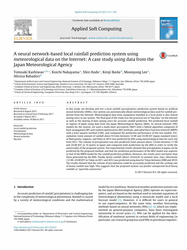
The proposed system aims at using data on the Internet as “bigdata” for rainfall prediction (Fig. 1). If efficient meteorological datacan be obtained from the Internet and shared among users, rainfallprediction can be made more accurate. One of the most efficienttypes of data for rainfall prediction in Japan is past meteorologicaldata from the Japan Meteorological Agency (JMA) [47]. In first stepof our research, data from the JMA was used for rainfall prediction.
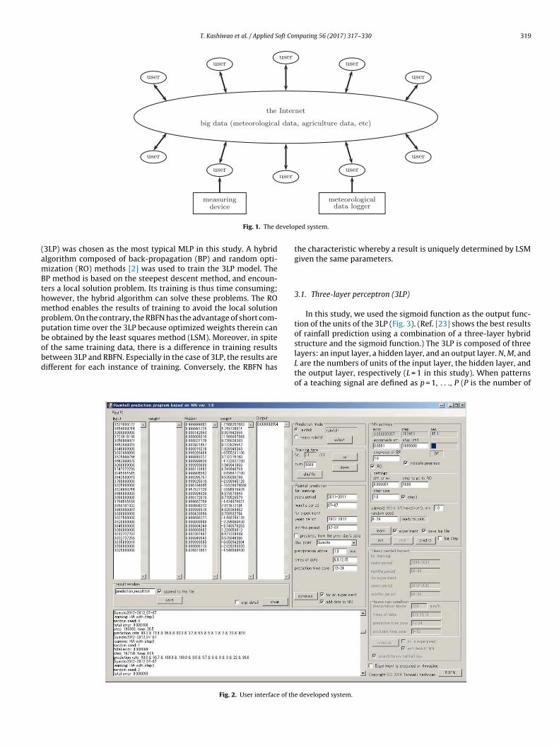
The proposed system could automatically obtain meteorologicaldata from the JMA website. We could easily change the condi-tions for meteorological data (date, time, and observation point)via the graphical user interface of our system (Fig. 2), developedin Microsoft Visual C# 2010. Moreover, the training of the NNs aswell as rainfall prediction was accomplished without complicatedoperations. In the next step, data from equipment installed at alocal point was used for rainfall prediction at each point. Meteoro-logical data at our college (National Institute of Technology (NIT),Niihama college, Ehime, Japan) is now being collected by using ameteorological data logger.
The use of big data on the Internet must be effective and effi-cient for rainfall prediction in terms of prediction accuracy andconvenience of collecting data. However, choosing an appropri-ate selection method for data is a challenging problem becausethere are massive amounts of relevant data on the Internet. NNshave been used for the analysis and sorting of big data. In partic-ular, “deep-learning” technology based on NNs is one of the mosteffective methods to this end [48]. In this study, we need to collectdata related to precipitation in each local spot that we analyzedfrom the Internet. However, if the data items are too numerous, NNtraining and computation become difficult and time-consuming.Therefore, an appropriate number of data items that can ensureprediction accuracy must be selected from the collected data. Inthe final stage of the study, we will use deep-learning technologyto collect and select big data on the Internet for rainfall predictionbased on the proposed method. (The kinds of effective meteorologydata are different for each local area due to differences in meteo-rological conditions, such as a location and topography. Thus, theselection of suitable data for each local spot is an important factorfor local rainfall prediction.)
3. Neural networks
In this section, we explain and compare the NN models used forour rainfall prediction experiment. General NN models—namely, amulti-layer perceptron (MLP) and a radial basis function network(RBFN)—were used for rainfall modeling. A three-layer perceptron
T. Kashiwao et al. / Applied Soft Computing 56 (2017) 317–330 319
evelo
(amBthmppbobd
Fig. 1. The d
3LP) was chosen as the most typical MLP in this study. A hybridlgorithm composed of back-propagation (BP) and random opti-ization (RO) methods [2] was used to train the 3LP model. The
P method is based on the steepest descent method, and encoun-ers a local solution problem. Its training is thus time consuming;owever, the hybrid algorithm can solve these problems. The ROethod enables the results of training to avoid the local solution
roblem. On the contrary, the RBFN has the advantage of short com-utation time over the 3LP because optimized weights therein cane obtained by the least squares method (LSM). Moreover, in spite
f the same training data, there is a difference in training resultsetween 3LP and RBFN. Especially in the case of 3LP, the results areifferent for each instance of training. Conversely, the RBFN hasFig. 2. User interface of th
ped system.
the characteristic whereby a result is uniquely determined by LSMgiven the same parameters.
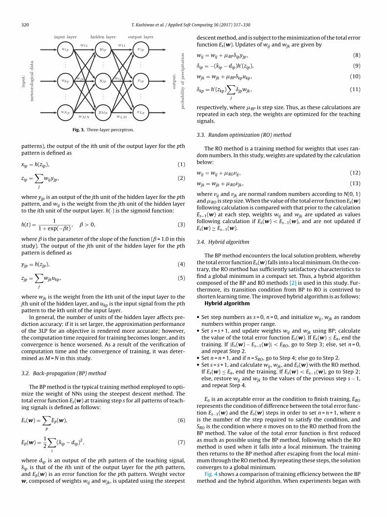
3.1. Three-layer perceptron (3LP)
In this study, we used the sigmoid function as the output func-tion of the units of the 3LP (Fig. 3). (Ref. [23] shows the best resultsof rainfall prediction using a combination of a three-layer hybridstructure and the sigmoid function.) The 3LP is composed of three
layers: an input layer, a hidden layer, and an output layer. N, M, andL are the numbers of units of the input layer, the hidden layer, andthe output layer, respectively (L = 1 in this study). When patternsof a teaching signal are defined as p = 1, . . ., P (P is the number ofe developed system.
320 T. Kashiwao et al. / Applied Soft Co
pp
x
z
wpt
h
wsp
y
z
wjp
dotccm
3
mti
E
E
wxaw
Fig. 3. Three-layer perceptron.
atterns), the output of the ith unit of the output layer for the pthattern is defined as
ip = h(zip), (1)
ip =∑j
wijyjp, (2)
here yjp is an output of the jth unit of the hidden layer for the pthattern, and wij is the weight from the jth unit of the hidden layero the ith unit of the output layer. h(·) is the sigmoid function:
(t) = 11 + exp(−ˇt) , > 0, (3)
here is the parameter of the slope of the function ( = 1.0 in thistudy). The output of the jth unit of the hidden layer for the pthattern is defined as
jp = h(zjp), (4)
jp =∑j
wjkukp, (5)
here wjk is the weight from the kth unit of the input layer to theth unit of the hidden layer, and ukp is the input signal from the pthattern to the kth unit of the input layer.
In general, the number of units of the hidden layer affects pre-iction accuracy: if it is set larger, the approximation performancef the 3LP for an objective is rendered more accurate; however,he computation time required for training becomes longer, and itsonvergence is hence worsened. As a result of the verification ofomputation time and the convergence of training, it was deter-ined as M = N in this study.
.2. Back-propagation (BP) method
The BP method is the typical training method employed to opti-ize the weight of NNs using the steepest descent method. The
otal error function Es(w) at training step s for all patterns of teach-ng signals is defined as follows:
s(w) =∑p
Ep(w), (6)
p(w) = 12
∑i
(xip − dip)2, (7)
here dip is an output of the pth pattern of the teaching signal,¯ ip is that of the ith unit of the output layer for the pth pattern,nd Ep(w) is an error function for the pth pattern. Weight vector, composed of weights wij and wjk, is updated using the steepest
mputing 56 (2017) 317–330
descent method, and is subject to the minimization of the total errorfunction Es(w). Updates of wij and wjk are given by
wij = wij + �BPıipyjp, (8)
ıip = −(xip − dip)h′(zip), (9)
wjk = wjk + �BPıkpukp, (10)
ıkp = h′(zkp)∑j
ıjpwjk, (11)
respectively, where �BP is step size. Thus, as these calculations arerepeated in each step, the weights are optimized for the teachingsignals.
3.3. Random optimization (RO) method
The RO method is a training method for weights that uses ran-dom numbers. In this study, weights are updated by the calculationbelow:
wij = wij + �ROvij, (12)
wjk = wjk + �ROvjk, (13)
where vij and vjk are normal random numbers according to N(0, 1)and �RO is step size. When the value of the total error function Es(w)following calculation is compared with that prior to the calculationEs−1(w) at each step, weights wij and wjk are updated as valuesfollowing calculation if Es(w) < Es−1(w), and are not updated ifEs(w) ≥ Es−1(w).
3.4. Hybrid algorithm
The BP method encounters the local solution problem, wherebythe total error function Es(w) falls into a local minimum. On the con-trary, the RO method has sufficiently satisfactory characteristics tofind a global minimum in a compact set. Thus, a hybrid algorithmcomposed of the BP and RO methods [2] is used in this study. Fur-thermore, its transition condition from BP to RO is contrived toshorten learning time. The improved hybrid algorithm is as follows:
Hybrid algorithm
• Set step numbers as s = 0, n = 0, and initialize wij, wjk as randomnumbers within proper range.
• Set s = s + 1, and update weights wij and wjk using BP; calculatethe value of the total error function Es(w). If Es(w) ≤ Ea, end thetraining. If |Es(w) − Es−1(w)| < ERO, go to Step 3; else, set n = 0,and repeat Step 2.
• Set n = n + 1, and if n = SRO, go to Step 4; else go to Step 2.• Set s = s + 1, and calculate wij , wjk, and Es(w) with the RO method.
If Es(w) ≤ Ea, end the training. If Es(w) < Es−1(w), go to Step 2;else, restore wij and wjk to the values of the previous step s − 1,and repeat Step 4.
Ea is an acceptable error as the condition to finish training, EROrepresents the condition of difference between the total error func-tion Es−1(w) and the Es(w) steps in order to set n = n + 1, where nis the number of the step required to satisfy the condition, andSRO is the condition where n moves on to the RO method from theBP method. The value of the total error function is first reducedas much as possible using the BP method, following which the ROmethod is used when it falls into a local minimum. The trainingthen returns to the BP method after escaping from the local mini-
mum through the RO method. By repeating these steps, the solutionconverges to a global minimum.Fig. 4 shows a comparison of training efficiency between the BPmethod and the hybrid algorithm. When experiments began with

T. Kashiwao et al. / Applied Soft Computing 56 (2017) 317–330 321
Fig. 4. Transition of the number of steps in the BP method and the hybrid algorithm(l
tciatS
ipwuotEimtsspSw
F3
Table 1Execution environment.
OS Windows 7 Professional 64 bitIDE Visual C# 2010 (Microsoft Visual Studio 2010)CPU Intel Core i7-3770 3.4 GHzRAM 16 GB
HA), which were plotted for 1000 steps (input layer: 32; hidden layer: 32; outputayer: 1; training data: 28).
he same initial parameters, the total error of the hybrid algorithmonverged to a smaller value than that of the BP method. The train-ng parameters were set as �BP = 1.0, �RO = 1.0, Ea = 10−4, Er = 10−6,nd SRO = 1000. In case training could not converge, it ended whenhe number of steps reached s = 106 in experiments described inections 4.3 and 5, and s = 5 × 10⁵ for the experiment in Section 4.4.
When the RO method was implemented on a program, the train-ng time was longer than that of the BP method, depending onrogramming language and execution environment, because alleights needed to be saved temporally when these weights were
pdated. Therefore, we added Step 3 in order to judge when to moven to the RO method from the conventional hybrid algorithm [2]. Ifhe training moved on to the RO method when |Es+1(w) − Es(w)| <
r in the Step 2 directory, the number of steps of the RO methodncreased, so that Step 3 had a function to adjust its frequency to
ove on to the RO method. In case the number of units was larger,he computation time required for training could be reduced if stepize �BP was set as the larger value and Step 3 was added. Fig. 5hows the graph of the relationship between the steps and the com-
utation time when training concluded with Step 3 and withouttep 3 under the execution conditions (Table 1). The experimentsith and without Step 3 began with the same initial parameters,ig. 5. Computation time of the hybrid algorithm (HA) with Step 3 and without Step (input layer: 32; hidden layer: 32; output layer: 1; training data: 28).
Fig. 6. RBF network.
and the results of 100 iterations were plotted for each (The averagesof computation times, Step 3: 1001 s; without Step 3: 1692 s).
3.5. Radial basis function network (RBFN)
RBFN is used to approximate a nonlinear function and rainfallprediction as well as MLP in [21]. The network structure of RBFN issimilar to that of 3LP (Fig. 6). However, a Gaussian function
�j(Up) = exp
(−‖Up − Uj‖2
2�2
)for j = 1, . . ., M, (14)
�M+1(Up) = 1, (15)
(Up)k = ukp, (16)
(Uj) = [uj, . . ., uj]�, (17)
is used as the output function for the units instead of the sigmoidfunction (Eq. (3)). Up ∈ RN and U ∈ RN are an output vector and acenter vector for the pth input pattern, respectively, uj ∈ R is thevalue of the center of the Gaussian function, which is allocatedto each unit of the hidden layer, � ∈ R is the standard deviation,�M+1(Up) is a bias, and ukp is an input signal for the kth unit of theinput layer for the pth input pattern.
From the output and weights of each unit of the hidden layer,the output of each unit of the output layer is represented as
xip =M+1∑j=1
wij�j(Up). (18)
If the center uj and standard deviation � are determined, the bestapproximation of the weight vector can be obtained by LSM at thesame time:
W� = �+X, (19)
�+ = (���)−1��, (20)
(W) = (wij), (21)
(�)pj = �j(Up), (22)
(X)pi = dip, (23)
322 T. Kashiwao et al. / Applied Soft Computing 56 (2017) 317–330
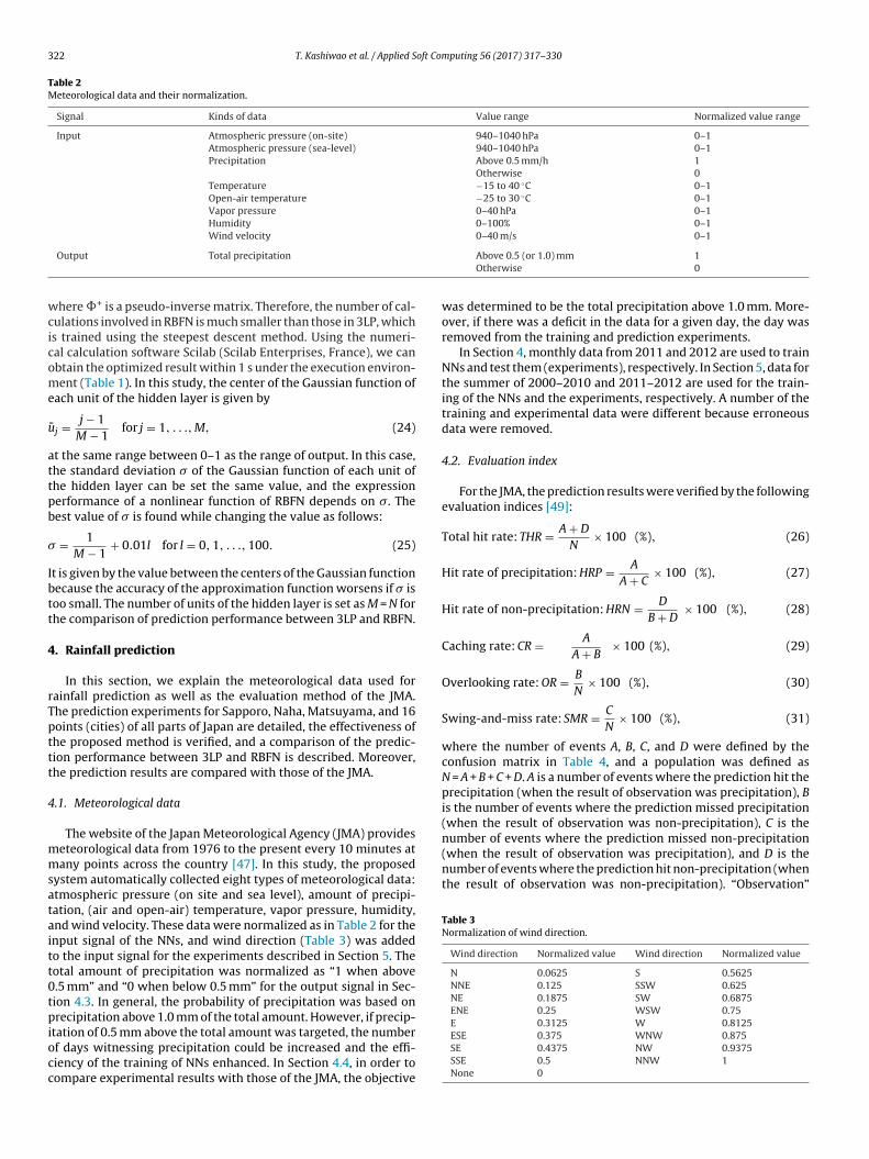
Table 2Meteorological data and their normalization.
Signal Kinds of data Value range Normalized value range
Input Atmospheric pressure (on-site) 940–1040 hPa 0–1Atmospheric pressure (sea-level) 940–1040 hPa 0–1Precipitation Above 0.5 mm/h 1
Otherwise 0Temperature −15 to 40 ◦C 0–1Open-air temperature −25 to 30 ◦C 0–1Vapor pressure 0–40 hPa 0–1Humidity 0–100% 0–1Wind velocity 0–40 m/s 0–1
wcicome
u
attpb
�
Ibtt
4
rTpttt
4
mmsataitt0tpiocc
number of events where the prediction missed non-precipitation(when the result of observation was precipitation), and D is thenumber of events where the prediction hit non-precipitation (whenthe result of observation was non-precipitation). “Observation”
Table 3Normalization of wind direction.
Wind direction Normalized value Wind direction Normalized value
N 0.0625 S 0.5625NNE 0.125 SSW 0.625NE 0.1875 SW 0.6875ENE 0.25 WSW 0.75E 0.3125 W 0.8125
Output Total precipitation
here �+ is a pseudo-inverse matrix. Therefore, the number of cal-ulations involved in RBFN is much smaller than those in 3LP, whichs trained using the steepest descent method. Using the numeri-al calculation software Scilab (Scilab Enterprises, France), we canbtain the optimized result within 1 s under the execution environ-ent (Table 1). In this study, the center of the Gaussian function of
ach unit of the hidden layer is given by
¯ j = j − 1M − 1
for j = 1, . . ., M, (24)
t the same range between 0–1 as the range of output. In this case,he standard deviation � of the Gaussian function of each unit ofhe hidden layer can be set the same value, and the expressionerformance of a nonlinear function of RBFN depends on �. Theest value of � is found while changing the value as follows:
= 1M − 1
+ 0.01l for l = 0, 1, . . ., 100. (25)
t is given by the value between the centers of the Gaussian functionecause the accuracy of the approximation function worsens if � isoo small. The number of units of the hidden layer is set as M = N forhe comparison of prediction performance between 3LP and RBFN.
. Rainfall prediction
In this section, we explain the meteorological data used forainfall prediction as well as the evaluation method of the JMA.he prediction experiments for Sapporo, Naha, Matsuyama, and 16oints (cities) of all parts of Japan are detailed, the effectiveness ofhe proposed method is verified, and a comparison of the predic-ion performance between 3LP and RBFN is described. Moreover,he prediction results are compared with those of the JMA.
.1. Meteorological data
The website of the Japan Meteorological Agency (JMA) provideseteorological data from 1976 to the present every 10 minutes atany points across the country [47]. In this study, the proposed
ystem automatically collected eight types of meteorological data:tmospheric pressure (on site and sea level), amount of precipi-ation, (air and open-air) temperature, vapor pressure, humidity,nd wind velocity. These data were normalized as in Table 2 for thenput signal of the NNs, and wind direction (Table 3) was addedo the input signal for the experiments described in Section 5. Theotal amount of precipitation was normalized as “1 when above.5 mm” and “0 when below 0.5 mm” for the output signal in Sec-ion 4.3. In general, the probability of precipitation was based onrecipitation above 1.0 mm of the total amount. However, if precip-
tation of 0.5 mm above the total amount was targeted, the numberf days witnessing precipitation could be increased and the effi-iency of the training of NNs enhanced. In Section 4.4, in order toompare experimental results with those of the JMA, the objective
Above 0.5 (or 1.0) mm 1Otherwise 0
was determined to be the total precipitation above 1.0 mm. More-over, if there was a deficit in the data for a given day, the day wasremoved from the training and prediction experiments.
In Section 4, monthly data from 2011 and 2012 are used to trainNNs and test them (experiments), respectively. In Section 5, data forthe summer of 2000–2010 and 2011–2012 are used for the train-ing of the NNs and the experiments, respectively. A number of thetraining and experimental data were different because erroneousdata were removed.
4.2. Evaluation index
For the JMA, the prediction results were verified by the followingevaluation indices [49]:
Total hit rate: THR = A + D
N× 100 (%), (26)
Hit rate of precipitation: HRP = A
A + C× 100 (%), (27)
Hit rate of non-precipitation: HRN = D
B + D× 100 (%), (28)
Caching rate:CR = A
A + B× 100 (%), (29)
Overlooking rate: OR = B
N× 100 (%), (30)
Swing-and-miss rate: SMR = C
N× 100 (%), (31)
where the number of events A, B, C, and D were defined by theconfusion matrix in Table 4, and a population was defined asN = A + B + C + D. A is a number of events where the prediction hit theprecipitation (when the result of observation was precipitation), Bis the number of events where the prediction missed precipitation(when the result of observation was non-precipitation), C is the
ESE 0.375 WNW 0.875SE 0.4375 NW 0.9375SSE 0.5 NNW 1None 0

T. Kashiwao et al. / Applied Soft Com
Table 4Confusion matrix of JMA.
Prediction
Precipitation Non-precipitation
Observation
hHhivctt
4
sfniicJnbJwio“
Precipitation A BNon-precipitation C D
ere means observed real weather. The higher the values of THR,RP, HRN, and CR, the better the prediction result. Contrarily, theigher the values of OR and SMR, the worse the prediction result. CR
s the most important value from the point of view of disaster pre-ention; however, the prediction becomes a case of “the boy whoried wolf” (whereby there exist many cases where the precipita-ion expected according to the prediction did not occur) if HRP wasoo low.
.3. Sapporo, Matsuyama, and Naha
The precipitation (total amount above 0.5 mm) in Sapporo, Mat-uyama, and Naha in 2012 was predicted by NNs trained with dataor the respective cities from 2011. In order to verify the effective-ess of the proposed method, Sapporo (the biggest city of Hokkaido
n the northern-most region of Japan), Matsuyama (the largest cityn Shikoku), and Naha (the southern-most big city in Japan) werehosen (Fig. 7). The data in Table 2 at 3:00, 6:00, 9:00, and 12:00ST (Japan standard time: UTC+9) was set as the input signal (totalumber: 32), and the output signal of the teaching signal was giveny the total amount of precipitation in the afternoon (12:00–24:00
ST). Precipitation for each day of each month at each city in 2012as predicted by NNs trained using data from the correspond-
ng month in 2011. The object precipitation was above 0.5 mmf the total amount. Thus, the prediction result was defined asprecipitation” if the total amount was above 0.5 mm, and as “non-
Fig. 7. Observation points in Japan (the map image from CraftMAP [50]).
puting 56 (2017) 317–330 323
precipitation” if the total amount was below 0.5 mm. A predictionresult was defined as “the precipitation when the output of NNs≥0.5” and “non-precipitation when the output of NNs <0.5.” In theexperiments, 30 of the 3LP NNs were trained while changing eachof the initial weights, and 101 of the RBFN NNs were trained whilechanging the standard deviation, as in Eq. (25).
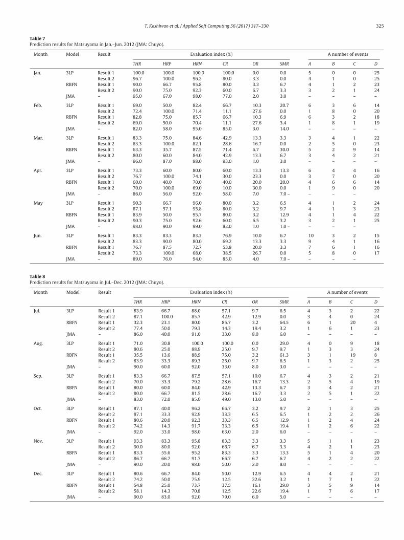
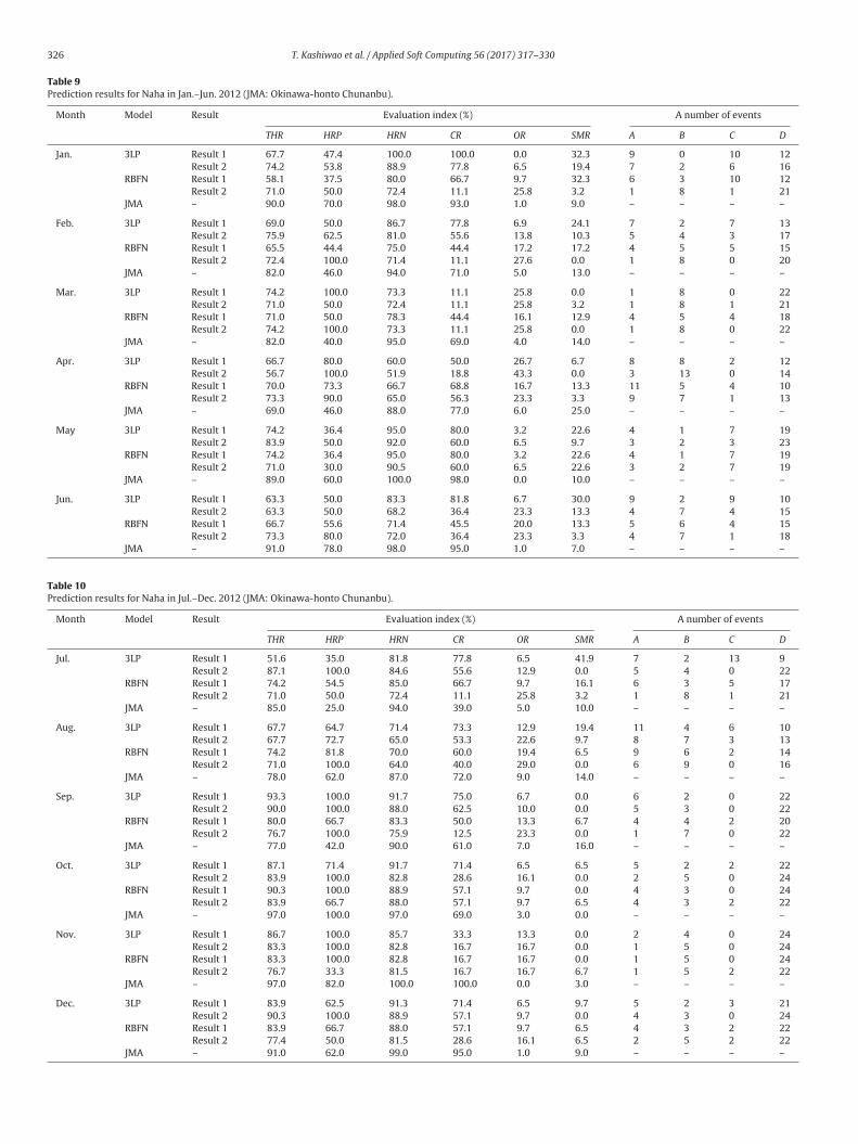
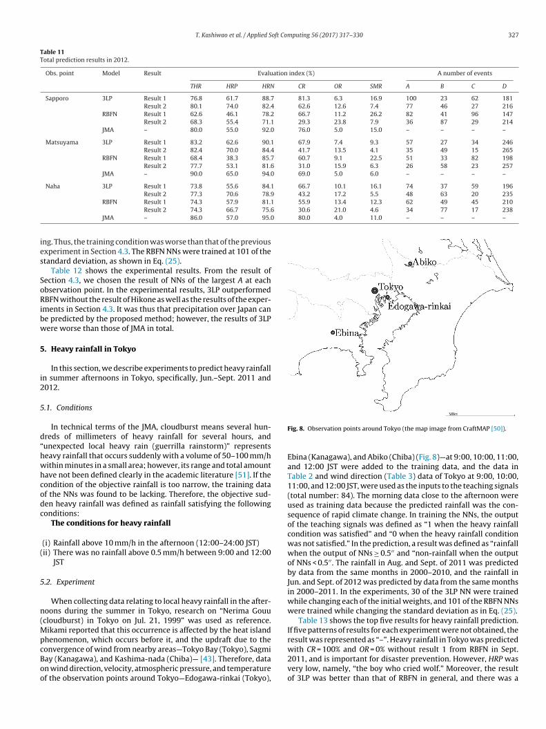
Tables 5–10 show the experimental results for Sapporo, Mat-suyama, and Naha. Result 1 shows the best prediction results fora number of A events, and result 2 represents the best predictionresults for a number of D events (if result 1 included the best resultof D, result 2 was the second-best result of A or D.) Moreover, resultsbiased toward precipitation or non-precipitation were removed.JMA in tables means the monthly average of the evaluation indicesin the JMA’s precipitation prediction for each area, including eachcity, which is listed on the organization’s website [49]. The object ofthe prediction was precipitation between 17:00 and 24:00 JST eachday, and was announced at 17:00 JST every day. The JMA’s resultsare shown as a reference value of the prediction rate. Table 11shows the total result for a year for each city.
The results for 3LP were better than those for RBFN in theexperiments in general. However, there were months where theprediction results for RBFN were better than those for 3LP. Fur-thermore, we observed that there were relationships involvingtrade-offs between the number of A and D events. The larger thenumber of events of type A, the smaller those of type D. On thecontrary, the larger the number of D events, the smaller that of Aevents. Moreover, HRP was low when A was large because the NNsof large A events tended to predict “precipitation” rather than “non-precipitation;” however, this implied the “the boy who cried wolf”results. Contrarily, the larger the number of D events, the higher HRPwas, and the lower CR was. Therefore, the NNs for large number ofA events needed to be chosen from the point of view of disasterprevention. Furthermore, the results were not considerably worsethan those of the JMA (however, it was not easy to compare theresults due to differences in conditions, such as time zone and sizeof object area).
4.4. 16 points in Japan
Precipitation for 16 points (cities) shown below in all regions ofJapan was predicted in order to verify the accuracy of the methodfor the country.
• Wakkanai and Asahikawa in Hokkaido• Aomori and Akita in Tohoku• Mito and Utsunomiya in Kanto• Sizuoka and Nagoya in Tokai• Niigata and Toyama in Hokuriku• Hikone in Kinki• Tokushima in Shikoku• Okayama and Shimonoseki in Chugoku• Miyazaki in Kyushu• Naha in Okinawa
For more accurate comparison with the JMA results, the con-ditions for the training data and the time zone of objectiveprecipitation were changed: the input signals for the teachingsignals were set as data at 6:00, 9:00, 12:00, and 15:00 JST(total number: 32), and the output signals of the teaching signalswere given by the total amount of precipitation in the afternoon(17:00–24:00 JST). The object was changed to precipitation above1.0 mm of the total amount because JMA’s prediction targeted the
total precipitation above 1.0 mm. In the experiments, 20 of the 3LPNNs were trained while changing the initial weights, and the con-dition for training step to end the training of 3LP was changed tos = 5 × 10⁵ from s = 106 in order to reduce the time needed for train-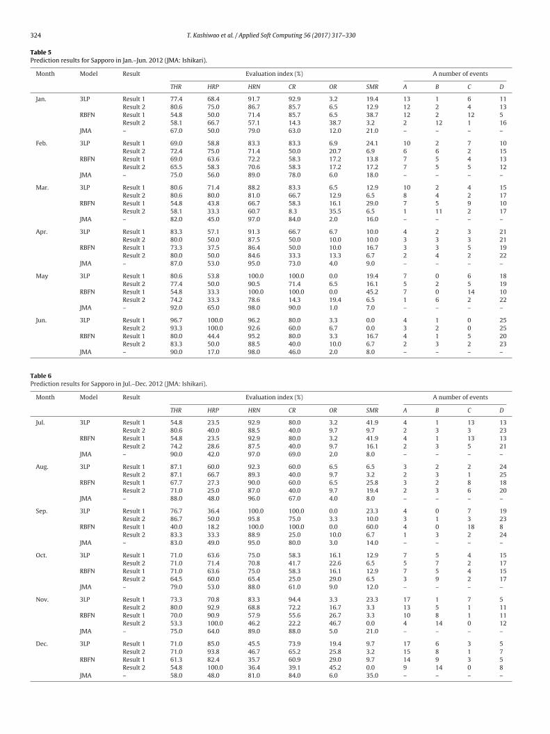
324 T. Kashiwao et al. / Applied Soft Computing 56 (2017) 317–330
Table 5Prediction results for Sapporo in Jan.–Jun. 2012 (JMA: Ishikari).
Month Model Result Evaluation index (%) A number of events
THR HRP HRN CR OR SMR A B C D
Jan. 3LP Result 1 77.4 68.4 91.7 92.9 3.2 19.4 13 1 6 11Result 2 80.6 75.0 86.7 85.7 6.5 12.9 12 2 4 13
RBFN Result 1 54.8 50.0 71.4 85.7 6.5 38.7 12 2 12 5Result 2 58.1 66.7 57.1 14.3 38.7 3.2 2 12 1 16
JMA – 67.0 50.0 79.0 63.0 12.0 21.0 – – – –
Feb. 3LP Result 1 69.0 58.8 83.3 83.3 6.9 24.1 10 2 7 10Result 2 72.4 75.0 71.4 50.0 20.7 6.9 6 6 2 15
RBFN Result 1 69.0 63.6 72.2 58.3 17.2 13.8 7 5 4 13Result 2 65.5 58.3 70.6 58.3 17.2 17.2 7 5 5 12
JMA – 75.0 56.0 89.0 78.0 6.0 18.0 – – – –
Mar. 3LP Result 1 80.6 71.4 88.2 83.3 6.5 12.9 10 2 4 15Result 2 80.6 80.0 81.0 66.7 12.9 6.5 8 4 2 17
RBFN Result 1 54.8 43.8 66.7 58.3 16.1 29.0 7 5 9 10Result 2 58.1 33.3 60.7 8.3 35.5 6.5 1 11 2 17
JMA – 82.0 45.0 97.0 84.0 2.0 16.0 – – – –
Apr. 3LP Result 1 83.3 57.1 91.3 66.7 6.7 10.0 4 2 3 21Result 2 80.0 50.0 87.5 50.0 10.0 10.0 3 3 3 21
RBFN Result 1 73.3 37.5 86.4 50.0 10.0 16.7 3 3 5 19Result 2 80.0 50.0 84.6 33.3 13.3 6.7 2 4 2 22
JMA – 87.0 53.0 95.0 73.0 4.0 9.0 – – – –
May 3LP Result 1 80.6 53.8 100.0 100.0 0.0 19.4 7 0 6 18Result 2 77.4 50.0 90.5 71.4 6.5 16.1 5 2 5 19
RBFN Result 1 54.8 33.3 100.0 100.0 0.0 45.2 7 0 14 10Result 2 74.2 33.3 78.6 14.3 19.4 6.5 1 6 2 22
JMA – 92.0 65.0 98.0 90.0 1.0 7.0 – – – –
Jun. 3LP Result 1 96.7 100.0 96.2 80.0 3.3 0.0 4 1 0 25Result 2 93.3 100.0 92.6 60.0 6.7 0.0 3 2 0 25
RBFN Result 1 80.0 44.4 95.2 80.0 3.3 16.7 4 1 5 20Result 2 83.3 50.0 88.5 40.0 10.0 6.7 2 3 2 23
JMA – 90.0 17.0 98.0 46.0 2.0 8.0 – – – –
Table 6Prediction results for Sapporo in Jul.–Dec. 2012 (JMA: Ishikari).
Month Model Result Evaluation index (%) A number of events
THR HRP HRN CR OR SMR A B C D
Jul. 3LP Result 1 54.8 23.5 92.9 80.0 3.2 41.9 4 1 13 13Result 2 80.6 40.0 88.5 40.0 9.7 9.7 2 3 3 23
RBFN Result 1 54.8 23.5 92.9 80.0 3.2 41.9 4 1 13 13Result 2 74.2 28.6 87.5 40.0 9.7 16.1 2 3 5 21
JMA – 90.0 42.0 97.0 69.0 2.0 8.0 – – – –
Aug. 3LP Result 1 87.1 60.0 92.3 60.0 6.5 6.5 3 2 2 24Result 2 87.1 66.7 89.3 40.0 9.7 3.2 2 3 1 25
RBFN Result 1 67.7 27.3 90.0 60.0 6.5 25.8 3 2 8 18Result 2 71.0 25.0 87.0 40.0 9.7 19.4 2 3 6 20
JMA – 88.0 48.0 96.0 67.0 4.0 8.0 – – – –
Sep. 3LP Result 1 76.7 36.4 100.0 100.0 0.0 23.3 4 0 7 19Result 2 86.7 50.0 95.8 75.0 3.3 10.0 3 1 3 23
RBFN Result 1 40.0 18.2 100.0 100.0 0.0 60.0 4 0 18 8Result 2 83.3 33.3 88.9 25.0 10.0 6.7 1 3 2 24
JMA – 83.0 49.0 95.0 80.0 3.0 14.0 – – – –
Oct. 3LP Result 1 71.0 63.6 75.0 58.3 16.1 12.9 7 5 4 15Result 2 71.0 71.4 70.8 41.7 22.6 6.5 5 7 2 17
RBFN Result 1 71.0 63.6 75.0 58.3 16.1 12.9 7 5 4 15Result 2 64.5 60.0 65.4 25.0 29.0 6.5 3 9 2 17
JMA – 79.0 53.0 88.0 61.0 9.0 12.0 – – – –
Nov. 3LP Result 1 73.3 70.8 83.3 94.4 3.3 23.3 17 1 7 5Result 2 80.0 92.9 68.8 72.2 16.7 3.3 13 5 1 11
RBFN Result 1 70.0 90.9 57.9 55.6 26.7 3.3 10 8 1 11Result 2 53.3 100.0 46.2 22.2 46.7 0.0 4 14 0 12
JMA – 75.0 64.0 89.0 88.0 5.0 21.0 – – – –
Dec. 3LP Result 1 71.0 85.0 45.5 73.9 19.4 9.7 17 6 3 5Result 2 71.0 93.8 46.7 65.2 25.8 3.2 15 8 1 7
RBFN Result 1 61.3 82.4 35.7 60.9 29.0 9.7 14 9 3 5Result 2 54.8 100.0 36.4 39.1 45.2 0.0 9 14 0 8
JMA – 58.0 48.0 81.0 84.0 6.0 35.0 – – – –
T. Kashiwao et al. / Applied Soft Computing 56 (2017) 317–330 325
Table 7Prediction results for Matsuyama in Jan.–Jun. 2012 (JMA: Chuyo).
Month Model Result Evaluation index (%) A number of events
THR HRP HRN CR OR SMR A B C D
Jan. 3LP Result 1 100.0 100.0 100.0 100.0 0.0 0.0 5 0 0 25Result 2 96.7 100.0 96.2 80.0 3.3 0.0 4 1 0 25
RBFN Result 1 90.0 66.7 95.8 80.0 3.3 6.7 4 1 2 23Result 2 90.0 75.0 92.3 60.0 6.7 3.3 3 2 1 24
JMA – 95.0 67.0 98.0 77.0 2.0 3.0 – – – –
Feb. 3LP Result 1 69.0 50.0 82.4 66.7 10.3 20.7 6 3 6 14Result 2 72.4 100.0 71.4 11.1 27.6 0.0 1 8 0 20
RBFN Result 1 82.8 75.0 85.7 66.7 10.3 6.9 6 3 2 18Result 2 69.0 50.0 70.4 11.1 27.6 3.4 1 8 1 19
JMA – 82.0 58.0 95.0 85.0 3.0 14.0 – – – –
Mar. 3LP Result 1 83.3 75.0 84.6 42.9 13.3 3.3 3 4 1 22Result 2 83.3 100.0 82.1 28.6 16.7 0.0 2 5 0 23
RBFN Result 1 63.3 35.7 87.5 71.4 6.7 30.0 5 2 9 14Result 2 80.0 60.0 84.0 42.9 13.3 6.7 3 4 2 21
JMA – 96.0 87.0 98.0 93.0 1.0 3.0 – – – –
Apr. 3LP Result 1 73.3 60.0 80.0 60.0 13.3 13.3 6 4 4 16Result 2 76.7 100.0 74.1 30.0 23.3 0.0 3 7 0 20
RBFN Result 1 60.0 40.0 70.0 40.0 20.0 20.0 4 6 6 14Result 2 70.0 100.0 69.0 10.0 30.0 0.0 1 9 0 20
JMA – 86.0 56.0 92.0 58.0 7.0 7.0 – – – –
May 3LP Result 1 90.3 66.7 96.0 80.0 3.2 6.5 4 1 2 24Result 2 87.1 57.1 95.8 80.0 3.2 9.7 4 1 3 23
RBFN Result 1 83.9 50.0 95.7 80.0 3.2 12.9 4 1 4 22Result 2 90.3 75.0 92.6 60.0 6.5 3.2 3 2 1 25
JMA – 98.0 90.0 99.0 82.0 1.0 1.0 – – – –
Jun. 3LP Result 1 83.3 83.3 83.3 76.9 10.0 6.7 10 3 2 15Result 2 83.3 90.0 80.0 69.2 13.3 3.3 9 4 1 16
RBFN Result 1 76.7 87.5 72.7 53.8 20.0 3.3 7 6 1 16Result 2 73.3 100.0 68.0 38.5 26.7 0.0 5 8 0 17
JMA – 89.0 76.0 94.0 85.0 4.0 7.0 – – – –
Table 8Prediction results for Matsuyama in Jul.–Dec. 2012 (JMA: Chuyo).
Month Model Result Evaluation index (%) A number of events
THR HRP HRN CR OR SMR A B C D
Jul. 3LP Result 1 83.9 66.7 88.0 57.1 9.7 6.5 4 3 2 22Result 2 87.1 100.0 85.7 42.9 12.9 0.0 3 4 0 24
RBFN Result 1 32.3 23.1 80.0 85.7 3.2 64.5 6 1 20 4Result 2 77.4 50.0 79.3 14.3 19.4 3.2 1 6 1 23
JMA – 86.0 40.0 91.0 33.0 8.0 6.0 – – – –
Aug. 3LP Result 1 71.0 30.8 100.0 100.0 0.0 29.0 4 0 9 18Result 2 80.6 25.0 88.9 25.0 9.7 9.7 1 3 3 24
RBFN Result 1 35.5 13.6 88.9 75.0 3.2 61.3 3 1 19 8Result 2 83.9 33.3 89.3 25.0 9.7 6.5 1 3 2 25
JMA – 90.0 60.0 92.0 33.0 8.0 3.0 – – – –
Sep. 3LP Result 1 83.3 66.7 87.5 57.1 10.0 6.7 4 3 2 21Result 2 70.0 33.3 79.2 28.6 16.7 13.3 2 5 4 19
RBFN Result 1 80.0 60.0 84.0 42.9 13.3 6.7 3 4 2 21Result 2 80.0 66.7 81.5 28.6 16.7 3.3 2 5 1 22
JMA – 83.0 72.0 85.0 49.0 13.0 5.0 – – – –
Oct. 3LP Result 1 87.1 40.0 96.2 66.7 3.2 9.7 2 1 3 25Result 2 87.1 33.3 92.9 33.3 6.5 6.5 1 2 2 26
RBFN Result 1 80.6 20.0 92.3 33.3 6.5 12.9 1 2 4 24Result 2 74.2 14.3 91.7 33.3 6.5 19.4 1 2 6 22
JMA – 92.0 33.0 98.0 63.0 2.0 6.0 – – – –
Nov. 3LP Result 1 93.3 83.3 95.8 83.3 3.3 3.3 5 1 1 23Result 2 90.0 80.0 92.0 66.7 6.7 3.3 4 2 1 23
RBFN Result 1 83.3 55.6 95.2 83.3 3.3 13.3 5 1 4 20Result 2 86.7 66.7 91.7 66.7 6.7 6.7 4 2 2 22
JMA – 90.0 20.0 98.0 50.0 2.0 8.0 – – – –
Dec. 3LP Result 1 80.6 66.7 84.0 50.0 12.9 6.5 4 4 2 21Result 2 74.2 50.0 75.9 12.5 22.6 3.2 1 7 1 22
RBFN Result 1 54.8 25.0 73.7 37.5 16.1 29.0 3 5 9 14Result 2 58.1 14.3 70.8 12.5 22.6 19.4 1 7 6 17
JMA – 90.0 83.0 92.0 79.0 6.0 5.0 – – – –
326 T. Kashiwao et al. / Applied Soft Computing 56 (2017) 317–330
Table 9Prediction results for Naha in Jan.–Jun. 2012 (JMA: Okinawa-honto Chunanbu).
Month Model Result Evaluation index (%) A number of events
THR HRP HRN CR OR SMR A B C D
Jan. 3LP Result 1 67.7 47.4 100.0 100.0 0.0 32.3 9 0 10 12Result 2 74.2 53.8 88.9 77.8 6.5 19.4 7 2 6 16
RBFN Result 1 58.1 37.5 80.0 66.7 9.7 32.3 6 3 10 12Result 2 71.0 50.0 72.4 11.1 25.8 3.2 1 8 1 21
JMA – 90.0 70.0 98.0 93.0 1.0 9.0 – – – –
Feb. 3LP Result 1 69.0 50.0 86.7 77.8 6.9 24.1 7 2 7 13Result 2 75.9 62.5 81.0 55.6 13.8 10.3 5 4 3 17
RBFN Result 1 65.5 44.4 75.0 44.4 17.2 17.2 4 5 5 15Result 2 72.4 100.0 71.4 11.1 27.6 0.0 1 8 0 20
JMA – 82.0 46.0 94.0 71.0 5.0 13.0 – – – –
Mar. 3LP Result 1 74.2 100.0 73.3 11.1 25.8 0.0 1 8 0 22Result 2 71.0 50.0 72.4 11.1 25.8 3.2 1 8 1 21
RBFN Result 1 71.0 50.0 78.3 44.4 16.1 12.9 4 5 4 18Result 2 74.2 100.0 73.3 11.1 25.8 0.0 1 8 0 22
JMA – 82.0 40.0 95.0 69.0 4.0 14.0 – – – –
Apr. 3LP Result 1 66.7 80.0 60.0 50.0 26.7 6.7 8 8 2 12Result 2 56.7 100.0 51.9 18.8 43.3 0.0 3 13 0 14
RBFN Result 1 70.0 73.3 66.7 68.8 16.7 13.3 11 5 4 10Result 2 73.3 90.0 65.0 56.3 23.3 3.3 9 7 1 13
JMA – 69.0 46.0 88.0 77.0 6.0 25.0 – – – –
May 3LP Result 1 74.2 36.4 95.0 80.0 3.2 22.6 4 1 7 19Result 2 83.9 50.0 92.0 60.0 6.5 9.7 3 2 3 23
RBFN Result 1 74.2 36.4 95.0 80.0 3.2 22.6 4 1 7 19Result 2 71.0 30.0 90.5 60.0 6.5 22.6 3 2 7 19
JMA – 89.0 60.0 100.0 98.0 0.0 10.0 – – – –
Jun. 3LP Result 1 63.3 50.0 83.3 81.8 6.7 30.0 9 2 9 10Result 2 63.3 50.0 68.2 36.4 23.3 13.3 4 7 4 15
RBFN Result 1 66.7 55.6 71.4 45.5 20.0 13.3 5 6 4 15Result 2 73.3 80.0 72.0 36.4 23.3 3.3 4 7 1 18
JMA – 91.0 78.0 98.0 95.0 1.0 7.0 – – – –
Table 10Prediction results for Naha in Jul.–Dec. 2012 (JMA: Okinawa-honto Chunanbu).
Month Model Result Evaluation index (%) A number of events
THR HRP HRN CR OR SMR A B C D
Jul. 3LP Result 1 51.6 35.0 81.8 77.8 6.5 41.9 7 2 13 9Result 2 87.1 100.0 84.6 55.6 12.9 0.0 5 4 0 22
RBFN Result 1 74.2 54.5 85.0 66.7 9.7 16.1 6 3 5 17Result 2 71.0 50.0 72.4 11.1 25.8 3.2 1 8 1 21
JMA – 85.0 25.0 94.0 39.0 5.0 10.0 – – – –
Aug. 3LP Result 1 67.7 64.7 71.4 73.3 12.9 19.4 11 4 6 10Result 2 67.7 72.7 65.0 53.3 22.6 9.7 8 7 3 13
RBFN Result 1 74.2 81.8 70.0 60.0 19.4 6.5 9 6 2 14Result 2 71.0 100.0 64.0 40.0 29.0 0.0 6 9 0 16
JMA – 78.0 62.0 87.0 72.0 9.0 14.0 – – – –
Sep. 3LP Result 1 93.3 100.0 91.7 75.0 6.7 0.0 6 2 0 22Result 2 90.0 100.0 88.0 62.5 10.0 0.0 5 3 0 22
RBFN Result 1 80.0 66.7 83.3 50.0 13.3 6.7 4 4 2 20Result 2 76.7 100.0 75.9 12.5 23.3 0.0 1 7 0 22
JMA – 77.0 42.0 90.0 61.0 7.0 16.0 – – – –
Oct. 3LP Result 1 87.1 71.4 91.7 71.4 6.5 6.5 5 2 2 22Result 2 83.9 100.0 82.8 28.6 16.1 0.0 2 5 0 24
RBFN Result 1 90.3 100.0 88.9 57.1 9.7 0.0 4 3 0 24Result 2 83.9 66.7 88.0 57.1 9.7 6.5 4 3 2 22
JMA – 97.0 100.0 97.0 69.0 3.0 0.0 – – – –
Nov. 3LP Result 1 86.7 100.0 85.7 33.3 13.3 0.0 2 4 0 24Result 2 83.3 100.0 82.8 16.7 16.7 0.0 1 5 0 24
RBFN Result 1 83.3 100.0 82.8 16.7 16.7 0.0 1 5 0 24Result 2 76.7 33.3 81.5 16.7 16.7 6.7 1 5 2 22
JMA – 97.0 82.0 100.0 100.0 0.0 3.0 – – – –
Dec. 3LP Result 1 83.9 62.5 91.3 71.4 6.5 9.7 5 2 3 21Result 2 90.3 100.0 88.9 57.1 9.7 0.0 4 3 0 24
RBFN Result 1 83.9 66.7 88.0 57.1 9.7 6.5 4 3 2 22Result 2 77.4 50.0 81.5 28.6 16.1 6.5 2 5 2 22
JMA – 91.0 62.0 99.0 95.0 1.0 9.0 – – – –
T. Kashiwao et al. / Applied Soft Computing 56 (2017) 317–330 327
Table 11Total prediction results in 2012.
Obs. point Model Result Evaluation index (%) A number of events
THR HRP HRN CR OR SMR A B C D
Sapporo 3LP Result 1 76.8 61.7 88.7 81.3 6.3 16.9 100 23 62 181Result 2 80.1 74.0 82.4 62.6 12.6 7.4 77 46 27 216
RBFN Result 1 62.6 46.1 78.2 66.7 11.2 26.2 82 41 96 147Result 2 68.3 55.4 71.1 29.3 23.8 7.9 36 87 29 214
JMA – 80.0 55.0 92.0 76.0 5.0 15.0 – – – –
Matsuyama 3LP Result 1 83.2 62.6 90.1 67.9 7.4 9.3 57 27 34 246Result 2 82.4 70.0 84.4 41.7 13.5 4.1 35 49 15 265
RBFN Result 1 68.4 38.3 85.7 60.7 9.1 22.5 51 33 82 198Result 2 77.7 53.1 81.6 31.0 15.9 6.3 26 58 23 257
JMA – 90.0 65.0 94.0 69.0 5.0 6.0 – – – –
Naha 3LP Result 1 73.8 55.6 84.1 66.7 10.1 16.1 74 37 59 196Result 2 77.3 70.6 78.9 43.2 17.2 5.5 48 63 20 235
55.9 13.4 12.3 62 49 45 210 30.6 21.0 4.6 34 77 17 238
80.0 4.0 11.0 – – – –
ies
SoRibw
5
i2
5
d“hwhcodc
(
5
n(MpcBoo
RBFN Result 1 74.3 57.9 81.1Result 2 74.3 66.7 75.6
JMA – 86.0 57.0 95.0
ng. Thus, the training condition was worse than that of the previousxperiment in Section 4.3. The RBFN NNs were trained at 101 of thetandard deviation, as shown in Eq. (25).
Table 12 shows the experimental results. From the result ofection 4.3, we chosen the result of NNs of the largest A at eachbservation point. In the experimental results, 3LP outperformedBFN without the result of Hikone as well as the results of the exper-
ments in Section 4.3. It was thus that precipitation over Japan cane predicted by the proposed method; however, the results of 3LPere worse than those of JMA in total.
. Heavy rainfall in Tokyo
In this section, we describe experiments to predict heavy rainfalln summer afternoons in Tokyo, specifically, Jun.–Sept. 2011 and012.
.1. Conditions
In technical terms of the JMA, cloudburst means several hun-reds of millimeters of heavy rainfall for several hours, andunexpected local heavy rain (guerrilla rainstorm)” representseavy rainfall that occurs suddenly with a volume of 50–100 mm/hithin minutes in a small area; however, its range and total amount
ave not been defined clearly in the academic literature [51]. If theondition of the objective rainfall is too narrow, the training dataf the NNs was found to be lacking. Therefore, the objective sud-en heavy rainfall was defined as rainfall satisfying the followingonditions:
The conditions for heavy rainfall
(i) Rainfall above 10 mm/h in the afternoon (12:00–24:00 JST)ii) There was no rainfall above 0.5 mm/h between 9:00 and 12:00
JST
.2. Experiment
When collecting data relating to local heavy rainfall in the after-oons during the summer in Tokyo, research on “Nerima Gouucloudburst) in Tokyo on Jul. 21, 1999” was used as reference.
ikami reported that this occurrence is affected by the heat islandhenomenon, which occurs before it, and the updraft due to the
onvergence of wind from nearby areas—Tokyo Bay (Tokyo), Sagmiay (Kanagawa), and Kashima-nada (Chiba)— [43]. Therefore, datan wind direction, velocity, atmospheric pressure, and temperaturef the observation points around Tokyo—Edogawa-rinkai (Tokyo),Fig. 8. Observation points around Tokyo (the map image from CraftMAP [50]).
Ebina (Kanagawa), and Abiko (Chiba) (Fig. 8)—at 9:00, 10:00, 11:00,and 12:00 JST were added to the training data, and the data inTable 2 and wind direction (Table 3) data of Tokyo at 9:00, 10:00,11:00, and 12:00 JST, were used as the inputs to the teaching signals(total number: 84). The morning data close to the afternoon wereused as training data because the predicted rainfall was the con-sequence of rapid climate change. In training the NNs, the outputof the teaching signals was defined as “1 when the heavy rainfallcondition was satisfied” and “0 when the heavy rainfall conditionwas not satisfied.” In the prediction, a result was defined as “rainfallwhen the output of NNs ≥ 0.5′′ and “non-rainfall when the outputof NNs < 0.5′′. The rainfall in Aug. and Sept. of 2011 was predictedby data from the same months in 2000–2010, and the rainfall inJun. and Sept. of 2012 was predicted by data from the same monthsin 2000–2011. In the experiments, 30 of the 3LP NN were trainedwhile changing each of the initial weights, and 101 of the RBFN NNswere trained while changing the standard deviation as in Eq. (25).
Table 13 shows the top five results for heavy rainfall prediction.If five patterns of results for each experiment were not obtained, theresult was represented as “–”. Heavy rainfall in Tokyo was predictedwith CR = 100% and OR = 0% without result 1 from RBFN in Sept.
2011, and is important for disaster prevention. However, HRP wasvery low, namely, “the boy who cried wolf.” Moreover, the resultof 3LP was better than that of RBFN in general, and there was a
328 T. Kashiwao et al. / Applied Soft Computing 56 (2017) 317–330
Table 12Averages prediction results for 2012.
Obs. point Model Evaluation index (%) A number of events
THR HRP HRN CR OR SMR A B C D
Wakkanai (Souya) 3LP 83.3 64.9 88.0 57.8 9.6 7.1 48 35 26 257RBFN 75.1 45.2 84.0 45.8 12.3 12.6 38 45 46 237JMA 80.0 55.0 92.0 76.0 5.0 15.0 – – – –
Asahikawa (Kamikawa) 3LP 78.4 51.6 87.8 59.8 9.0 12.6 49 33 46 237RBFN 71.0 39.1 84.7 52.4 10.7 18.4 43 39 67 216JMA 81.0 58.0 92.0 76.0 6.0 13.0 – – – –
Aomori (Aomori Tsugaru) 3LP 78.1 50.9 90.8 72.0 6.3 15.6 59 23 57 227RBFN 74.9 44.6 85.0 50.0 11.2 13.9 41 41 51 233JMA 81.0 58.0 95.0 86.0 3.0 15.0 – – – –
Akita (Akita Engan) 3LP 81.6 61.0 87.6 58.8 9.6 8.8 50 35 32 248RBFN 73.2 43.7 84.7 52.9 11.0 15.9 45 40 58 222JMA 81.0 61.0 94.0 86.0 4.0 15.0 – – – –
Mito (Ibaragi Hokubu) 3LP 85.5 52.6 91.6 53.6 7.1 7.4 30 26 27 282RBFN 79.5 37.0 90.1 48.2 7.9 12.6 27 29 46 263JMA 90.0 65.0 97.0 86.0 2.0 7.0 – – – –
Utsunomiya (Tochigi Nanbu) 3LP 86.6 58.9 91.6 55.9 7.1 6.3 33 26 23 284RBFN 78.7 38.0 89.9 50.8 7.9 13.4 30 29 49 258JMA 90.0 64.0 97.0 84.0 3.0 8.0 – – – –
Shizuoka (Shizuoka Chubu) 3LP 87.7 63.8 91.2 51.7 7.7 4.7 30 28 17 290RBFN 69.9 25.9 88.3 48.3 8.2 21.9 28 30 80 227JMA 92.0 78.0 95.0 78.0 4.0 4.0 – – – –
Nagoya (Aichi Seibu) 3LP 90.4 60.0 95.2 66.7 4.1 5.5 30 15 20 300RBFN 84.1 40.3 94.0 60.0 4.9 11.0 27 18 40 280JMA 92.0 66.0 98.0 91.0 1.0 6.0 – – – –
Niigata (Niigata Kaetsu) 3LP 82.7 62.5 89.1 64.7 8.2 9.1 55 30 33 246RBFN 73.1 43.6 84.4 51.8 11.3 15.7 44 41 57 222JMA 87.0 75.0 94.0 86.0 4.0 5.0 – – – –
Toyama (Toyama Toubu) 3LP 77.3 57.4 88.2 72.5 7.7 15.0 74 28 55 209RBFN 74.6 53.5 85.8 66.7 9.3 16.1 68 34 59 205JMA 86.0 73.0 94.0 88.0 4.0 10.0 – – – –
Hikone (Shiga Hokubu) 3LP 84.1 54.2 89.9 50.8 8.5 7.4 32 31 27 275RBFN 76.4 38.6 90.9 61.9 6.6 17.0 39 24 62 240JMA 85.0 63.0 94.0 84.0 4.0 11.0 – – – –
Okayama (Okayama Nanbu) 3LP 89.9 50.0 95.6 62.2 3.8 6.3 23 14 23 306RBFN 87.7 42.0 94.9 56.8 4.4 7.9 21 16 29 300JMA 94.0 72.0 97.0 75.0 3.0 3.0 – – – –
Shimonoseki (Yamaguchi Seibu) 3LP 81.4 36.8 93.1 58.3 5.5 13.1 28 20 48 270RBFN 82.2 36.5 91.7 47.9 6.8 10.9 23 25 40 278JMA 91.0 64.0 97.0 82.0 2.0 6.0 – – – –
Tokushima (Tokushima Hokubu) 3LP 89.5 56.8 94.0 56.8 5.2 5.2 25 19 19 300RBFN 79.9 26.2 90.7 36.4 7.7 12.4 16 28 45 274JMA 85.0 51.0 93.0 65.0 5.0 10.0 – – – –
Miyazaki (Miyazaki Nanbu–heiyabu) 3LP 88.8 71.8 93.4 74.7 5.2 6.0 56 19 22 268RBFN 79.2 49.4 87.7 53.3 9.6 11.2 40 35 41 249JMA 89.0 74.0 93.0 76.0 5.0 6.0 – – – –
89.989.795.0
ta
6
mecfiTop
Naha (Okinawa–honto Chunanbu) 3LP 77.9 41.1
RBFN 80.9 46.7
JMA 86.0 57.0
rade-off relationship between A and D in the result of 3LP in Aug.nd Sept., 2011, as well as in the experiment in Section 4.3.
. Conclusion and future work
This paper proposed local rainfall prediction based on NNs usingeteorological data obtained from the website of the JMA. The
ffectiveness of JMA data for local rainfall prediction in Japan wasonfirmed. The precipitation of Sapporo, Matsuyama, and Naha was
rst predicted, followed by precipitation at 16 points over Japan.he prediction results were compared with the JMA’s results. Webserved that the proposed method was outperformed by JMA’srediction. Finally, heavy rainfall in summer afternoons in Tokyo56.9 7.7 14.5 37 28 53 248 53.8 8.2 10.9 35 30 40 261
80.0 4.0 11.0 – – – –
was predicted, and the results suggested the possibility of theprediction of unexpected local heavy rainfall as “guerrilla rain-storms”. From these results, it can be shown that 3LP is betterthan RBFN for the precipitation prediction problem, and there isa trade-off relationship between the hit rate of precipitation A andnon-precipitation D. In this study, the number of trained NNs was20 or 30 for 3LP and 101 for RBFN in the experiments. We canconclude that NNs are better trained and more accurate for predic-tion if these numbers are increased in value. Furthermore, better
machine-learning models need to be investigated to improve pre-diction performance (e.g., support vector machines and randomforest). Furthermore, an investigation is needed into the methodused to choose meteorological data because suitable data can be
T. Kashiwao et al. / Applied Soft Computing 56 (2017) 317–330 329
Table 13Prediction results of heavy rainfall in Tokyo in 2011 and 2012.
Month Model Result Evaluation indices (%) A number of events
THR HRP HRN CR OR SMR A B C D
Aug. 2011 3LP Result 1 80.6 33.3 100.0 100.0 0.0 19.4 3 0 6 22Result 2 77.4 30.0 100.0 100.0 0.0 22.6 3 0 7 21Result 3 80.6 28.6 95.8 66.7 3.2 16.1 2 1 5 23Result 4 77.4 25.0 95.7 66.7 3.2 19.4 2 1 6 22Result 5 74.2 22.2 95.5 66.7 3.2 22.6 2 1 7 21
RBFN Result 1 67.7 23.1 100.0 100.0 0.0 32.3 3 0 10 18Result 2 64.5 21.4 100.0 100.0 0.0 35.5 3 0 11 17Result 3 61.3 20.0 100.0 100.0 0.0 38.7 3 0 12 16Result 4 58.1 18.8 100.0 100.0 0.0 41.9 3 0 13 15Result 5 51.6 16.7 100.0 100.0 0.0 48.4 3 0 15 13
Sep. 2011 3LP Result 1 79.3 25.0 100.0 100.0 0.0 20.7 2 0 6 21Result 2 27.6 8.7 100.0 100.0 0.0 72.4 2 0 21 6Result 3 82.8 20.0 95.8 50.0 3.4 13.8 1 1 4 23Result 4 79.3 16.7 95.7 50.0 3.4 17.2 1 1 5 22Result 5 75.9 14.3 95.5 50.0 3.4 20.7 1 1 6 21
RBFN Result 1 51.7 7.1 93.3 50.0 3.4 44.8 1 1 13 14Result 2 48.3 6.7 92.9 50.0 3.4 48.3 1 1 14 13Result 3 44.8 6.3 92.3 50.0 3.4 51.7 1 1 15 12Result 4 – – – – – – – – – –Result 5 – – – – – – – – – –
Jun. 2012 3LP Result 1 90.0 25.0 100.0 100.0 0.0 10.0 1 0 3 26Result 2 83.3 16.7 100.0 100.0 0.0 16.7 1 0 5 24Result 3 76.7 12.5 100.0 100.0 0.0 23.3 1 0 7 22Result 4 73.3 11.1 100.0 100.0 0.0 26.7 1 0 8 21Result 5 70.0 10.0 100.0 100.0 0.0 30.0 1 0 9 20
RBFN Result 1 53.3 6.7 100.0 100.0 0.0 46.7 1 0 14 15Result 2 46.7 5.9 100.0 100.0 0.0 53.3 1 0 16 13Result 3 43.3 5.6 100.0 100.0 0.0 56.7 1 0 17 12Result 4 36.7 5.0 100.0 100.0 0.0 63.3 1 0 19 10Result 5 30.0 4.5 100.0 100.0 0.0 70.0 1 0 21 8
Sep. 2012 3LP Result 1 75.9 22.2 100.0 100.0 0.0 24.1 2 0 7 20Result 2 72.4 20.0 100.0 100.0 0.0 27.6 2 0 8 19Result 3 62.1 15.4 100.0 100.0 0.0 37.9 2 0 11 16Result 4 55.2 13.3 100.0 100.0 0.0 44.8 2 0 13 14Result 5 44.8 11.1 100.0 100.0 0.0 55.2 2 0 16 11
RBFN Result 1 69.0 18.2 100.0 100.0 0.0 31.0 2 0 9 18Result 2 65.5 16.7 100.0 100.0 0.0 34.5 2 0 10 17
.0
.0
.0
dorfabp
ltscitlt
A
nAh
[
Result 3 62.1 15.4 100Result 4 58.6 14.3 100Result 5 55.2 13.3 100
ifferent among prediction points due to the difference in the effectf conditions, such as altitude, ocean current, airflow, etc. The accu-ate prediction of precipitation, namely, larger A, is most importantrom the point of view of disaster prevention; however, it can cause
situation of the “the boy who cried wolf.” Therefore, the compati-ility of both the prediction of precipitation and non-precipitationersists as an issue for future research.
In future work, we plan to predict local precipitation based onocal data obtained from a meteorological data logger installed athe NIT, Niihama College (Ehime, Japan). Moreover, a system tohare data among users (such as individuals, schools, universities,ompanies, etc.) via the Internet will be developed. If meteorolog-cal data around the prediction point can be shared with users,he accuracy of prediction can be improved. Moreover, data col-ection and selection methods from big data using deep-learningechnology will be developed to improve the developed system.
cknowledgments
This work was supported by the National Institute of Tech-ology, Niihama College, Japan, and Southern Cross University,ustralia. We are grateful to Prof. Koichi Suzuki, Prof. Shuji Sako-ara, Prof. Mikio Deguchi, and Prof. Scott T. Smith for their support.
[
100.0 0.0 37.9 2 0 11 16100.0 0.0 41.4 2 0 12 15100.0 0.0 44.8 2 0 13 14
References
[1] JMA, JMA numerical weather prediction, http://www.jma.go.jp/jma/jma-eng/jma-center/nwp/nwp-top.htm (16.07.15).
[2] B. Norio, K. Fumio, O. Seiichi, Foundations of Neural Networks andApplications, Kyoritsu Shuppan, 1994 (in Japanese).
[3] G.P. Liu, Nonlinear Identification and Control: A NEURAL network Approach,Springer Science & Business Media, 2012.
[4] B. Norio, T. Masahiro, Y. Yasunari, M. Yasue, H. Hisashi, Foundations of SoftComputing and Applications, Kyoritsu Shuppan, Tokyo, Japan, 2012 (inJapanese). https://books.google.com.au/books?id=AMfBuAAACAAJ.
[5] A.J. Maren, C.T. Harston, R.M. Pap, Handbook of Neural ComputingApplications, Academic Press, 2014.
[6] D.R. Nayak, A. Mahapatra, P. Mishra, A survey on rainfall prediction usingartificial neural network, Int. J. Comput. Appl. 72 (16) (2013).
[7] M.A. Ahmadi, R. Soleimani, M. Lee, T. Kashiwao, A. Bahadori, Determination ofoil well production performance using artificial neural network (ANN) linkedto the particle swarm optimization (PSO) tool, Petroleum 1 (2) (2015)118–132.
[8] A. Tatar, S. Naseri, M. Bahadori, J. Rozyn, M. Lee, T. Kashiwao, A. Bahadori,Evaluation of different artificial intelligent models to predict reservoirformation water density, Pet. Sci. Technol. 33 (20) (2015) 1749–1756.
[9] M. Ahmadi, T. Kashiwao, A. Bahadori, Prediction of oil production rate usingvapor-extraction technique in heavy oil recovery operations, Pet. Sci. Technol.33 (20) (2015) 1764–1769.
10] A. Tatar, A. Shokrollahi, M. Lee, T. Kashiwao, A. Bahadori, Prediction ofsupercritical CO2/brine relative permeability in sedimentary basins during
carbon dioxide sequestration, Greenh. Gases Sci. Technol. 5 (6) (2015)756–771.11] S. Naseri, A. Tatar, M. Bahadori, J. Rozyn, T. Kashiwao, A. Bahadori, Applicationof radial basis function neural network for prediction of titration-basedasphaltene precipitation, Pet. Sci. Technol. 33 (23-24) (2015) 1875–1882.

3 oft Co
[
[
[
[
[
[
[
[
[
[
[
[
[
[
[
[
[
[
[
[
[
[
[
[
[
[
[
[
[
[
[
[
[
[
[
[
[
[49] JMA, Results of accuracy verification of a weather forecast, http://www.data.jma.go.jp/fcd/yoho/kensho/yohohyoka top.html (in Japanese) (16.07.15).
[50] CraftMAP, http://www.craftmap.box-i.net/ (in Japanese) (01.07.15).
30 T. Kashiwao et al. / Applied S
12] E. Soroush, M. Mesbah, A. Shokrollahi, J. Rozyn, M. Lee, T. Kashiwao, A.Bahadori, Evolving a robust modeling tool for prediction of natural gashydrate formation conditions, J. Unconv. Oil Gas Resour. 12 (2015) 45–55.
13] M. Ahmadi, T. Kashiwao, J. Rozyn, A. Bahadori, Accurate prediction ofproperties of carbon dioxide for carbon capture and sequestration operations,Pet. Sci. Technol. 34 (1) (2016) 97–103.
14] Z. Ahmad, J. Zhang, T. Kashiwao, A. Bahadori, Prediction of absorption andstripping factors in natural gas processing industries using feedforwardartificial neural network, Pet. Sci. Technol. 34 (2) (2016) 105–113.
15] A. Bahadori, A. Baghban, M. Bahadori, T. Kashiwao, M.V. Ayouri, Estimation ofemission of hydrocarbons and filling losses in storage containers usingintelligent models, Pet. Sci. Technol. 34 (2) (2016) 145–152.
16] M. Ahmadi, T. Kashiwao, M. Bahadori, A. Bahadori, Estimation ofwater-hydrocarbon mutual solubility in gas processing operations using anintelligent model, Pet. Sci. Technol. 34 (4) (2016) 328–334.
17] A. Tatar, A. Najafi-Marghmaleki, A. Barati-Harooni, A. Gholami, H. Ansari, M.Bahadori, T. Kashiwao, M. Lee, A. Bahadori, Implementing radial basisfunction neural networks for prediction of saturation pressure of crude oils,Pet. Sci. Technol. 34 (5) (2016) 454–463.
18] J.S. Amin, A. Bahadori, T. Kashiwao, Z. Ahmad, B.A. Souraki, S. Rafiee, A newempirical correlation for prediction of carbon dioxide separation fromdifferent gas mixtures, Pet. Sci. Technol. 34 (6) (2016) 562–569.
19] A. Baghban, M. Bahadori, T. Kashiwao, A. Bahadori, Modelling of gas tohydrate conversion for promoting CO2 capture processes in the oil and gasindustry, Pet. Sci. Technol. 34 (7) (2016) 642–651.
20] J.S. Amin, M. Bahadori, M. Lee, T. Kashiwao, A. Bahadori, S. Rafiee, B.H. Nia,Prediction of carbon dioxide separation from gas mixtures in petroleumindustries using the Levenberg–Marquardt algorithm, Pet. Sci. Technol. 34 (8)(2016) 703–711.
21] S. Lee, S. Cho, P.M. Wong, Rainfall prediction using artificial neural networks,J. Geogr. Inf. Decis. Anal. 2 (2) (1998) 233–242.
22] K. Koizumi, An objective method to modify numerical model forecasts withnewly given weather data using an artificial neural network, WeatherForecast. 14 (1) (1999) 109–118.
23] K. Koizumi, M. Hirasawa, A neural-network structure suitable forprecipitation amount forecast, TENKI 48 (12) (2001) 885–892 (in Japanese).
24] K.C. Luk, J.E. Ball, A. Sharma, An application of artificial neural networks forrainfall forecasting, Math. Comput. Model. 33 (6) (2001) 683–693.
25] S. Ito, Y. Mitsukura, M. Fukumi, N. Akamatsu, Neuro rainfall forecast with datamining by real-coded genetical preprocessing, IEEJ Trans. Electron. Inf. Syst.123 (2003) 817–822 (in Japanese).
26] N.Q. Hung, M.S. Babel, S. Weesakul, N. Tripathi, An artificial neural networkmodel for rainfall forecasting in Bangkok, Thailand, Hydrol. Earth Syst. Sci. 13(8) (2009) 1413–1425.
27] K. Abhishek, A. Kumar, R. Ranjan, S. Kumar, A rainfall prediction model usingartificial neural network, in: Control and System Graduate ResearchColloquium (ICSGRC), 2012 IEEE, IEEE, 2012, pp. 82–87.
28] J. Abbot, J. Marohasy, Application of artificial neural networks to rainfallforecasting in Queensland, Australia, Adv. Atmos. Sci. 29 (4) (2012) 717–730.
29] P. Singh, B. Borah, Indian summer monsoon rainfall prediction using artificialneural network, Stoch. Environ. Res. Risk Assess. 27 (7) (2013) 1585–1599.
30] A. Alqudah, V. Chandrasekar, M. Le, Investigating rainfall estimation from
radar measurements using neural networks, Nat. Hazards Earth Syst. Sci. 13(3) (2013) 535–544.31] S. Koumura, Y. Matsuda, Y. Sekine, Y. Shidama, H. Yamaura, Local weatherprediction system by neural networks. IEICE technical report,Neurocomputing 94 (182) (1994) 25–32 (in Japanese).
[
mputing 56 (2017) 317–330
32] C. Dawson, R. Wilby, Hydrological modelling using artificial neural networks,Prog. Phys. Geogr. 25 (1) (2001) 80–108.
33] Y.B. Dibike, D.P. Solomatine, River flow forecasting using artificial neuralnetworks, Phys. Chem. Earth Part B: Hydrol. Oceans Atmos. 26 (1) (2001) 1–7.
34] H.K. Cigizoglu, M. Alp, Rainfall-runoff modelling using three neural networkmethods, in: Artificial Intelligence and Soft Computing-ICAISC 2004, Springer,2004, pp. 166–171.
35] A. Senthil Kumar, K. Sudheer, S. Jain, P. Agarwal, Rainfall-runoff modellingusing artificial neural networks: comparison of network types, Hydrol.Process. 19 (6) (2005) 1277–1291.
36] M. Shoaib, A.Y. Shamseldin, B.W. Melville, Comparative study of differentwavelet based neural network models for rainfall-runoff modeling, J. Hydrol.515 (2014) 47–58.
37] M. Zare, H.R. Pourghasemi, M. Vafakhah, B. Pradhan, Landslide susceptibilitymapping at VAZ watershed (Iran) using an artificial neural network model: acomparison between multilayer perceptron (MLP) and radial basic function(RBF) algorithms, Arab. J. Geosci. 6 (8) (2013) 2873–2888.
38] T. Kashiwao, S. Ando, K. Ikeda, T. Shimomura, Neural network-based localprediction of rainfall using meteorological data on the internet), Trans. Inst.Syst., Control Inf. Eng. 28 (3) (2015) 123–125 (in Japanese).
39] J. Manyika, M. Chui, B. Brown, J. Bughin, R. Dobbs, C. Roxburgh, A.H. Byers, Bigdata: the next frontier for innovation, competition, and productivity, 2011.
40] A. McAfee, E. Brynjolfsson, T.H. Davenport, D. Patil, D. Barton, Big data, themanagement revolution, Harv. Bus. Rev. 90 (10) (2012) 61–67.
41] Y.-G. Jung, H. Jin, Experimental comparisons of neural networks and logisticregression models for heart disease prediction, Information 16 (2) (2013).
42] B.C. Pijanowski, A. Tayyebi, J. Doucette, B.K. Pekin, D. Braun, J. Plourde, A bigdata urban growth simulation at a national scale: configuring the GIS andneural network based land transformation model to run in a highperformance computing (HPC) environment, Environ. Model. Softw. 51(2014) 250–268.
43] T. Mikami, H. Yamamoto, H. Ando, H. Yokoyama, T. Yamaguchi, M. Ichino, Y.Akiyama, K. Ishii, Climatological study on the summer intensive heavy rainfallin Tokyo, Annu. Rep. Tokyo Metrop. Res. Inst. Environ. Protect. 2005 (2005)33–42 (in Japanese).
44] T. Yamanaka, R. Ooka, Analysis of urban effect on local heavy rainfall in Tokyousing mesoscale model, The seventh International Conference on UrbanClimate (2009).
45] T. Kawabata, T. Kuroda, H. Seko, K. Saito, A cloud-resolving 4DVARassimilation experiment for a local heavy rainfall event in the Tokyometropolitan area, Mon. Weather Rev. 139 (6) (2011) 1911–1931.
46] K. Souma, K. Sunada, T. Suetsugi, K. Tanaka, Use of ensemble simulations toevaluate the urban effect on a localized heavy rainfall event in Tokyo, Japan, J.Hydroenviron. Res. 7 (4) (2013) 228–235.
47] JMA, Meteorological observation data,http://www.jma.go.jp/jma/menu/obsmenu.html (in Japanese) (1 Jul. 2015).
48] D. Erhan, Y. Bengio, A. Courville, P.-A. Manzagol, P. Vincent, S. Bengio, Whydoes unsupervised pre-training help deep learning? J. Mach. Learn. Res. 11(2010) 625–660.
51] JMA, Precipitation, http://www.jma.go.jp/jma/kishou/know/yougo hp/kousui.html (in Japanese) (16.07.15).
Top Related