


Languages
Pages
Legal

Applications of Matrix FunctionsPart III: Quantum Chemistry
Michele Benzi
Emory UniversityDepartment of Mathematics and Computer Science
Atlanta, GA 30322, USA
Michele Benzi Applications of Matrix Functions Part III: Quantum ChemistryLille, SSMF2013
Prologue
The main purpose of this lecture is to present a rigorous mathematical
theory for a class of methods, called O(N) methods, that are being
developed by computational physicists and chemists for the solution of the
electronic structure problem, which is fundamental to quantum chemistry,
solid state physics, biology, etc.
The theory is based on general results on the decay in the entries of
functions of sparse matrices. In particular, one needs to study the
asymptotic behavior of the off-diagonal matrix elements for N → ∞.
While this work is primarily theoretical, the theory can be used to
construct better algorithms for electronic structure computations. Some of
our techniques are already used in a code called FreeON developed by a
group headed by Matt Challacombe at Los Alamos National Laboratory.
Michele Benzi Applications of Matrix Functions Part III: Quantum ChemistryLille, SSMF2013

References
This lecture is based in parts on the results contained in the following
papers:
M. Benzi and G. H. Golub, Bounds for the entries of matrix functions with
applications to preconditioning, BIT, 39 (1999), pp. 417–438.
M. Benzi and N. Razouk, Decay bounds and O(n) algorithms for approximating
functions of sparse matrices, Electr. Trans. Numer. Anal., 28 (2007), pp. 16–39.
M. Benzi, P. Boito and N. Razouk, Decay properties of spectral projectors with
applications to electronic structure, SIAM Review, 55 (2013), pp. 3–64.
Michele Benzi Applications of Matrix Functions Part III: Quantum ChemistryLille, SSMF2013
Overview
1 The electronic structure problem
2 Density matrices
3 O(N) methods
4 A mathematical foundation for O(N) methods
5 O(N) approximation of functions of sparse matrices
6 A few numerical experiments
7 Some open problems
Michele Benzi Applications of Matrix Functions Part III: Quantum ChemistryLille, SSMF2013
The Electronic Structure Problem
A fundamental problem in quantum chemistry and solid state physics is to
determine the electronic structure of (possibly large) atomic and molecular
systems.
The problem amounts to computing the ground state (smallest eigenvalue
and corresponding eigenfunction) of the many-body quantum-mechanical
Hamiltonian (Schrodinger operator), H.
Variationally, we want to minimize the Rayleigh quotient:
E0 = minΨ6=0
〈HΨ,Ψ〉〈Ψ,Ψ〉
and Ψ0 = argminΨ6=0〈HΨ,Ψ〉〈Ψ,Ψ〉
where 〈·, ·〉 denotes the L2 inner product.
Michele Benzi Applications of Matrix Functions Part III: Quantum ChemistryLille, SSMF2013

The Electronic Structure Problem
Michele Benzi Applications of Matrix Functions Part III: Quantum ChemistryLille, SSMF2013

The Electronic Structure Problem
In the Born-Oppenheimer approximation, the many-body Hamiltonian (in
atomic units) is given by
H =
N∑i=1
−1
2∆i −
M∑j=1
Zj
|xi − rj |+
N∑j 6=i
1
|xi − xj |
where N = number of electrons and M = number of nuclei in the system.
The operator H acts on a suitable subspace D(H) ⊂ L2(R3N), the
antisymmetrized tensor product of N copies of H1(R3):
D(H) = H1(R3) ∧ . . .∧ H1(R3) .
This is because electrons are Fermions and therefore subject to Pauli’s
Exclusion Principle. Hence, the wavefunction must be antisymmetric:
Ψ(x1, . . . ,xi , . . . ,xj , . . . ,xN) = −Ψ(x1, . . . ,xj , . . . ,xi , . . . ,xN).
NOTE: To simplify notation, spin is ignored here.
Michele Benzi Applications of Matrix Functions Part III: Quantum ChemistryLille, SSMF2013

The Electronic Structure Problem
In the Born-Oppenheimer approximation, the many-body Hamiltonian (in
atomic units) is given by
H =
N∑i=1
−1
2∆i −
M∑j=1
Zj
|xi − rj |+
N∑j 6=i
1
|xi − xj |
where N = number of electrons and M = number of nuclei in the system.
The operator H acts on a suitable subspace D(H) ⊂ L2(R3N), the
antisymmetrized tensor product of N copies of H1(R3):
D(H) = H1(R3) ∧ . . .∧ H1(R3) .
This is because electrons are Fermions and therefore subject to Pauli’s
Exclusion Principle. Hence, the wavefunction must be antisymmetric:
Ψ(x1, . . . ,xi , . . . ,xj , . . . ,xN) = −Ψ(x1, . . . ,xj , . . . ,xi , . . . ,xN).
NOTE: To simplify notation, spin is ignored here.Michele Benzi Applications of Matrix Functions Part III: Quantum ChemistryLille, SSMF2013
The Electronic Structure Problem
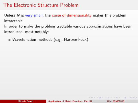
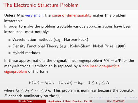
Unless N is very small, the curse of dimensionality makes this problem
intractable.
In order to make the problem tractable various approximations have been
introduced, most notably:
Wavefunction methods (e.g., Hartree-Fock)
Density Functional Theory (e.g., Kohn-Sham; Nobel Prize, 1998)
Hybrid methods
In these approximations the original, linear eigenproblem HΨ = EΨ for the
many-electrons Hamiltonian is replaced by a nonlinear one-particle
eigenproblem of the form
F (ψi ) = λiψi , 〈ψi , ψj〉 = δij , 1 ≤ i , j ≤ N
where λ1 ≤ λ2 ≤ · · · ≤ λN . This problem is nonlinear because the operator
F depends nonlinearly on the ψi .
Michele Benzi Applications of Matrix Functions Part III: Quantum ChemistryLille, SSMF2013

The Electronic Structure Problem
Unless N is very small, the curse of dimensionality makes this problem
intractable.
In order to make the problem tractable various approximations have been
introduced, most notably:
Wavefunction methods (e.g., Hartree-Fock)
Density Functional Theory (e.g., Kohn-Sham; Nobel Prize, 1998)
Hybrid methods
In these approximations the original, linear eigenproblem HΨ = EΨ for the
many-electrons Hamiltonian is replaced by a nonlinear one-particle
eigenproblem of the form
F (ψi ) = λiψi , 〈ψi , ψj〉 = δij , 1 ≤ i , j ≤ N
where λ1 ≤ λ2 ≤ · · · ≤ λN . This problem is nonlinear because the operator
F depends nonlinearly on the ψi .
Michele Benzi Applications of Matrix Functions Part III: Quantum ChemistryLille, SSMF2013
The Electronic Structure Problem
Unless N is very small, the curse of dimensionality makes this problem
intractable.
In order to make the problem tractable various approximations have been
introduced, most notably:
Wavefunction methods (e.g., Hartree-Fock)
Density Functional Theory (e.g., Kohn-Sham; Nobel Prize, 1998)
Hybrid methods
In these approximations the original, linear eigenproblem HΨ = EΨ for the
many-electrons Hamiltonian is replaced by a nonlinear one-particle
eigenproblem of the form
F (ψi ) = λiψi , 〈ψi , ψj〉 = δij , 1 ≤ i , j ≤ N
where λ1 ≤ λ2 ≤ · · · ≤ λN . This problem is nonlinear because the operator
F depends nonlinearly on the ψi .Michele Benzi Applications of Matrix Functions Part III: Quantum ChemistryLille, SSMF2013
The Electronic Structure Problem
Roughly speaking, in DFT the idea is to consider a single electron moving
in the electric field generated by the nuclei and by some average
distribution of the other electrons. Starting with an initial guess of the
charge density, a potential is formed and the corresponding one-particle
eigenproblem is solved; the resulting charge density is used to define the
new potential, and so on until the charge density no longer changes
appreciably.
More formally, DFT reformulates the problem so that the unknown
function is the electronic density
ρ(x) = N
∫R3(N−1)
|Ψ(x,x2, . . . ,xN)|2dx2 · · · dxN ,
a scalar field on R3.
The function ρ minimizes a certain functional, the form of which is not
known explicitly.
Michele Benzi Applications of Matrix Functions Part III: Quantum ChemistryLille, SSMF2013

The Electronic Structure Problem
Roughly speaking, in DFT the idea is to consider a single electron moving
in the electric field generated by the nuclei and by some average
distribution of the other electrons. Starting with an initial guess of the
charge density, a potential is formed and the corresponding one-particle
eigenproblem is solved; the resulting charge density is used to define the
new potential, and so on until the charge density no longer changes
appreciably.
More formally, DFT reformulates the problem so that the unknown
function is the electronic density
ρ(x) = N
∫R3(N−1)
|Ψ(x,x2, . . . ,xN)|2dx2 · · · dxN ,
a scalar field on R3.
The function ρ minimizes a certain functional, the form of which is not
known explicitly.Michele Benzi Applications of Matrix Functions Part III: Quantum ChemistryLille, SSMF2013
The Electronic Structure Problem
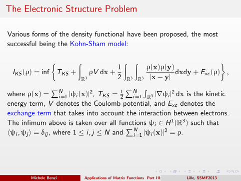
Various forms of the density functional have been proposed, the most
successful being the Kohn-Sham model:
IKS(ρ) = inf
{TKS +
∫R3
ρV dx +1
2
∫R3
∫R3
ρ(x)ρ(y)
|x − y|dxdy + Exc(ρ)
},
where ρ(x) =∑N
i=1 |ψi (x)|2, TKS = 12
∑Ni=1
∫R3 |∇ψi |
2 dx is the kinetic
energy term, V denotes the Coulomb potential, and Exc denotes the
exchange term that takes into account the interaction between electrons.
The infimum above is taken over all functions ψi ∈ H1(R3) such that
〈ψi , ψj〉 = δij , where 1 ≤ i , j ≤ N and∑N
i=1 |ψi (x)|2 = ρ.
This IKS is minimized with respect to ρ. Note that ρ, being the electron
density, must satisfy ρ > 0 and∫
R3 ρ dx = N.
Michele Benzi Applications of Matrix Functions Part III: Quantum ChemistryLille, SSMF2013

The Electronic Structure Problem
The Euler–Lagrange equations for this variational problem are the
Kohn–Sham equations:
F (ρ)ψi = λiψi , 〈ψi , ψj〉 = δij (1 ≤ i , j ≤ N)
with
F (ρ) = −1
2∆+ U(x, ρ)
where U denotes a (complicated) potential, and ρ =∑N
i=1 |ψi (x)|2.
Hence, the original intractable linear eigenvalue problem for the
many-body Hamiltonian is reduced to a tractable nonlinear eigenvalue
problem for a single-particle Hamiltonian.
Michele Benzi Applications of Matrix Functions Part III: Quantum ChemistryLille, SSMF2013

The Electronic Structure Problem
The nonlinear problem can be solved by a ‘self-consistent field’ (SCF)
iteration, leading to a sequence of linear eigenproblems
F (k)ψ(k)i = λ
(k)i ψ
(k)i , 〈ψ(k)
i , ψ(k)j 〉 = δij , k = 1, 2, . . .
(1 ≤ i , j ≤ N), where each F (k) = −12∆+ U(k) is a one-electron linearized
Hamiltonian:
U(k) = U(k)(x, ρ(k−1)), ρ(k−1) =
N∑i=1
|ψ(k−1)i (x)|2.
Solution of each of the (discretized) linear eigenproblems above leads
to a typical O(N3) cost per SCF iteration. However, the actual
eigenpairs (ψ(k)i , λ
(k)i ) are unnecessary, and diagonalization of the
one-particle Hamiltonians can be avoided!
Michele Benzi Applications of Matrix Functions Part III: Quantum ChemistryLille, SSMF2013
The Electronic Structure Problem
The individual eigenfunctions ψi are not needed. All one needs is the
orthogonal projector P onto the occupied subspace
Vocc = span{ψ1, . . . , ψN }
corresponding to the N lowest eigenvalues λ1 ≤ λ2 ≤ · · · ≤ λN .
At the kth SCF cycle, an approximation to the orthogonal projector P(k)
onto the occupied subspace V(k)occ needs to be computed.
All quantities of interest in electronic structure theory can be computed
from P. For example, the expected value for the total energy of the
system can be computed once P is known, as are the forces.
Higher moments of observables can also be computed once P is known.
Michele Benzi Applications of Matrix Functions Part III: Quantum ChemistryLille, SSMF2013

Overview
1 The electronic structure problem
2 Density matrices
3 O(N) methods
4 A mathematical foundation for O(N) methods
5 O(N) approximation of functions of sparse matrices
6 A few numerical experiments
7 Some open problems
Michele Benzi Applications of Matrix Functions Part III: Quantum ChemistryLille, SSMF2013
Density matrices
P is called the density operator of the system (von Neumann, 1927). For
systems in equilibrium, [H,P] = 0 and P is a function of the Hamiltonian:
P = f (H).
Density operators are sometimes normalized so that Tr(P) = 1.
In practice, the operators are replaced by matrices by Rayleigh-Ritz
projection onto a finite-dimensional subspace spanned by a set of basis
functions {φi }Nbi=1, where Nb is a multiple of N. Typically, N = C · Ne
where C ≥ 2 is a moderate integer when linear combinations of GTOs
(Gaussian-type orbitals) are used.
In some codes, plane waves are used. Finite difference and finite element
(“real space”) methods, while also used, are less popular.
Michele Benzi Applications of Matrix Functions Part III: Quantum ChemistryLille, SSMF2013
Density matrices
The Gramian matrix S = (Sij) where Sij = 〈φi , φj〉 is called the overlap
matrix in electronic structure. It is dense, but its entries fall off very
rapidly for increasing separation. In the case of GTOs:
|Sij | ≈ e−|i−j |2 , 1 ≤ i , j ≤ Nb .
Neglecting tiny entries leads to banded overlap matrices.
The density matrix P is the S-orthogonal projector onto the occupied
subspace. It is convenient to make a change of basis, from non-orthogonal
to orthogonal.
Trasforming the Hamiltonian H to an orthogonal basis means performing a
congruence trasformation: H = ZHZT , where Z is such that ZZT = S−1.
Common choices for Z are the inverse Cholesky factor of S or the inverse
square root S−1/2. This can be done efficiently (AINV algorithm).
Michele Benzi Applications of Matrix Functions Part III: Quantum ChemistryLille, SSMF2013
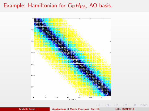
Example: Hamiltonian for C52H106, AO basis.
Michele Benzi Applications of Matrix Functions Part III: Quantum ChemistryLille, SSMF2013
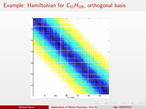
Example: Hamiltonian for C52H106, orthogonal basis
Michele Benzi Applications of Matrix Functions Part III: Quantum ChemistryLille, SSMF2013

Density matrices
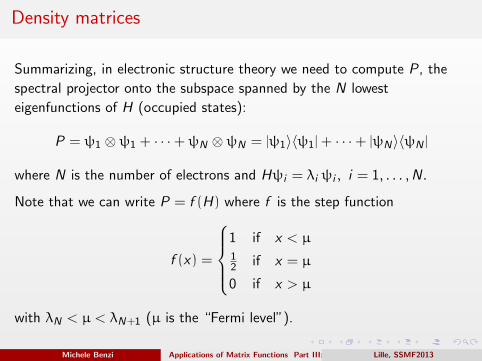
Summarizing, in electronic structure theory we need to compute P, the
spectral projector onto the subspace spanned by the N lowest
eigenfunctions of H (occupied states):
P = ψ1 ⊗ψ1 + · · ·+ψN ⊗ψN = |ψ1〉〈ψ1| + · · ·+ |ψN〉〈ψN |
where N is the number of electrons and Hψi = λi ψi , i = 1, . . . ,N.
Note that we can write P = f (H) where f is the step function
f (x) =
1 if x < µ12 if x = µ
0 if x > µ
with λN < µ < λN+1 (µ is the “Fermi level”).
Michele Benzi Applications of Matrix Functions Part III: Quantum ChemistryLille, SSMF2013
Density matrices
Summarizing, in electronic structure theory we need to compute P, the
spectral projector onto the subspace spanned by the N lowest
eigenfunctions of H (occupied states):
P = ψ1 ⊗ψ1 + · · ·+ψN ⊗ψN = |ψ1〉〈ψ1| + · · ·+ |ψN〉〈ψN |
where N is the number of electrons and Hψi = λi ψi , i = 1, . . . ,N.
Note that we can write P = f (H) where f is the step function
f (x) =
1 if x < µ12 if x = µ
0 if x > µ
with λN < µ < λN+1 (µ is the “Fermi level”).
Michele Benzi Applications of Matrix Functions Part III: Quantum ChemistryLille, SSMF2013

Overview
1 The electronic structure problem
2 Density matrices
3 O(N) methods
4 A mathematical foundation for O(N) methods
5 O(N) approximation of functions of sparse matrices
6 A few numerical experiments
7 Some open problems
Michele Benzi Applications of Matrix Functions Part III: Quantum ChemistryLille, SSMF2013

O(N) methods
Physicists have observed that the entries of the density matrix P decay
away from the main diagonal. The decay rate is algebraic for metallic
systems, and exponential (or faster) for insulators and semiconductors.
Hence, the density matrix is localized.
This property has been called nearsightedness by W. Kohn.
This property implies that in the thermodynamic limit (N → ∞ while
keeping the particle density constant) the number of entries Pij with
|Pij | > ε grows only linearly with N, for any prescribed ε > 0.
For insulators and semiconductors, this makes O(N) methods possible.
Michele Benzi Applications of Matrix Functions Part III: Quantum ChemistryLille, SSMF2013
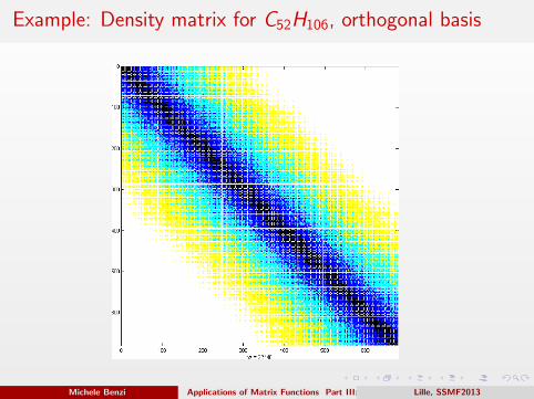
Example: Density matrix for C52H106, orthogonal basis
Michele Benzi Applications of Matrix Functions Part III: Quantum ChemistryLille, SSMF2013

Example: Density matrix for H = −12∆+ V , random V ,
finite differences (2D lattice), N = 10
020
4060
80100
0
20
40
60
80
1000
0.2
0.4
0.6
0.8
1
Michele Benzi Applications of Matrix Functions Part III: Quantum ChemistryLille, SSMF2013
O(N) methods
The fact that P is very nearly sparse allows the development of O(N)
approximation methods. Popular methods include
1 Chebyshev expansion: P = f (H) ≈ c02 +
∑nk=1 ckTk(H)
2 Rational expansions based on contour integration:
P =1
2πi
∫Γ(zI − H)−1dz ≈
q∑k=1
wk(zk I − H)−1
3 Density matrix minimization:
Tr(PH) = min, subject to P = P∗ = P2 and rank(P) = N
4 Etc. (see C. Le Bris, Acta Numerica, 2005; Bowler & Miyazaki, 2011)
All these methods can achieve O(N) scaling by exploiting “sparsity.”
Michele Benzi Applications of Matrix Functions Part III: Quantum ChemistryLille, SSMF2013

Overview
1 The electronic structure problem
2 Density matrices
3 O(N) methods
4 A mathematical foundation for O(N) methods
5 O(N) approximation of functions of sparse matrices
6 A few numerical experiments
7 Some open problems
Michele Benzi Applications of Matrix Functions Part III: Quantum ChemistryLille, SSMF2013
A mathematical foundation for O(N) methods
In literature one finds no rigorously proved, general results on the decay
behavior in P. Decay estimates are either non-rigorous (at least for a
mathematician!), or valid only for very special cases.
Goal: To establish rigorous estimates for the rate of decay in the
off-diagonal entries of P in the form of upper bounds on the entries of the
density matrix, in the thermodynamic limit N → ∞.
Ideally, these bounds can be used to provide cut-off rules, that is, to decide
which entries in P need not be computed, given a prescribed error
tolerance.
To achieve this goal we first need to find an appropriate formalization for
the type of problems encountered by physicists.
The main tool used in our analysis, besides linear algebra, is classical
approximation theory.
Michele Benzi Applications of Matrix Functions Part III: Quantum ChemistryLille, SSMF2013
A mathematical foundation for O(N) methods
Let C be a fixed positive integer and let Nb := C · N, where N → ∞. We
think of C as the number of basis functions per electron while N is the
number of electrons.
We call a sequence of discrete Hamiltonians a sequence of matrices {HN }
of order Nb, such that
1 The matrices HN have spectra uniformly bounded w.r.t. N: up to
shifting and scaling, we can assume σ(HN) ⊂ [−1, 1] for all N.
2 The HN are banded, with uniformly bounded bandwidth as N → ∞.
More generally, the HN are sparse with maximum number of nonzeros
per row bounded w.r.t. N.
These assumptions model the fact that the Hamiltonians have finite
interaction range, which remains bounded in the thermodynamic limit
N → ∞.
Michele Benzi Applications of Matrix Functions Part III: Quantum ChemistryLille, SSMF2013

A mathematical foundation for O(N) methods
Next, let H be a Hamiltonian of order Nb. Denote the eigenvalues of H as
−1 ≤ λ1 ≤ . . . ≤ λN < λN+1 ≤ . . . ≤ λNb≤ 1 .
The spectral gap is then γN = λN+1 − λN . In quantum chemistry this is
known as the HOMO-LUMO gap, in solid state physics as the band gap.
Two cases are possible:
1 There exists γ > 0 such that γN ≥ γ for all N.
2 infN γN = 0.
The first case corresponds to insulators and semiconductors, the second
one to metallic systems.
Michele Benzi Applications of Matrix Functions Part III: Quantum ChemistryLille, SSMF2013

Example: Spectrum of the Hamiltonian for C52H106.
0 100 200 300 400 500 600 700−1.5
−1
−0.5
0
0.5
1
1.5
index i
eig
en
va
lue
s ε
i
ε52
ε53
gap due to core electrons
HOMO−LUMO gapε209
ε210
Michele Benzi Applications of Matrix Functions Part III: Quantum ChemistryLille, SSMF2013

Exponential decay in the density matrix for gapped systems
Theorem
Let {HN } be a sequence of discrete Hamiltonians of size Nb = C · N, with
C constant and N → ∞. Let PN denote the spectral projector onto the N
occupied states associated with HN . If there exists γ > 0 such that the
gaps γN ≥ γ for all N, then there exists constants K and α such that
|[PN ]ij | ≤ K e−αdN (i ,j) (1 ≤ i , j ≤ N),
where dN(i , j) denotes the geodetic distance between node i and node j in
the graph GN associated with HN . The constants K and α depend only on
the gap γ (not on N) and are easily computable.
Note: The graph GN = (VN ,EN) is the graph with Nb vertices such that
there is an edge (i , j) ∈ EN if and only if [HN ]ij 6= 0.
Michele Benzi Applications of Matrix Functions Part III: Quantum ChemistryLille, SSMF2013
Exponential decay in the density matrix for gapped systems
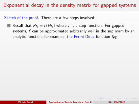
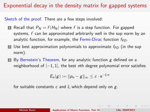
Sketch of the proof. There are a few steps involved:
1 Recall that PN = f (HN) where f is a step function. For gapped
systems, f can be approximated arbitrarily well in the sup norm by an
analytic function, for example, the Fermi-Dirac function fFD .
2 Use best approximation polynomials to approximate fFD (in the sup
norm).
3 By Bernstein’s Theorem, for any analytic function g defined on a
neighborhood of [−1, 1], the best nth degree polynomial error satisfies
En(g) := ‖pn − g‖∞ ≤ c · e−ξ n
for suitable constants c and ξ which depend only on g .
4 Apply Bernstein’s result to g = fFD , compute the decay constants,
and use the spectral theorem to go from scalars to matrices.
Michele Benzi Applications of Matrix Functions Part III: Quantum ChemistryLille, SSMF2013

Exponential decay in the density matrix for gapped systems
Sketch of the proof. There are a few steps involved:
1 Recall that PN = f (HN) where f is a step function. For gapped
systems, f can be approximated arbitrarily well in the sup norm by an
analytic function, for example, the Fermi-Dirac function fFD .
2 Use best approximation polynomials to approximate fFD (in the sup
norm).
3 By Bernstein’s Theorem, for any analytic function g defined on a
neighborhood of [−1, 1], the best nth degree polynomial error satisfies
En(g) := ‖pn − g‖∞ ≤ c · e−ξ n
for suitable constants c and ξ which depend only on g .
4 Apply Bernstein’s result to g = fFD , compute the decay constants,
and use the spectral theorem to go from scalars to matrices.
Michele Benzi Applications of Matrix Functions Part III: Quantum ChemistryLille, SSMF2013
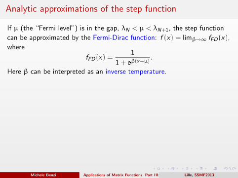
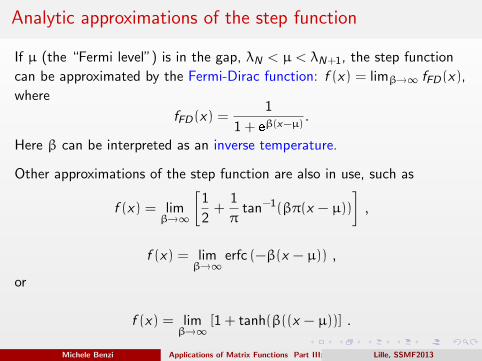
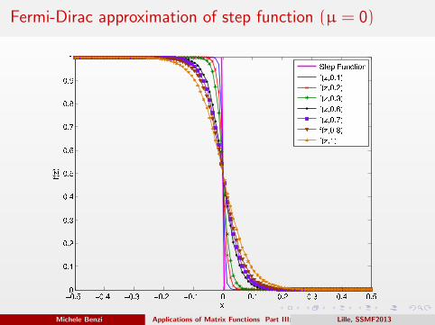
Analytic approximations of the step function
If µ (the “Fermi level”) is in the gap, λN < µ < λN+1, the step function
can be approximated by the Fermi-Dirac function: f (x) = limβ→∞ fFD(x),
where
fFD(x) =1
1 + eβ(x−µ)
.
Here β can be interpreted as an inverse temperature.
Other approximations of the step function are also in use, such as
f (x) = limβ→∞
[1
2+
1
πtan−1(βπ(x − µ))
],
f (x) = limβ→∞ erfc (−β(x − µ)) ,
or
f (x) = limβ→∞ [1 + tanh(β((x − µ))] .
Michele Benzi Applications of Matrix Functions Part III: Quantum ChemistryLille, SSMF2013
Fermi-Dirac approximation of step function (µ = 0)
Michele Benzi Applications of Matrix Functions Part III: Quantum ChemistryLille, SSMF2013
Fermi-Dirac approximation of step function
The actual choice of β in the Fermi-Dirac function is dictated by the size
of the gap γ and by the approximation error.
What is important is that for any prescribed error, there is a maximum
value of β that achieves the error for all N, provided the system has
non-vanishing gap.
On the other hand, for γ → 0 we have β → ∞ and the bounds blow up.
This happens for metals (at zero temperature).
There is still decay in the density matrix, but it may be algebraic rather
than exponential. Simple examples show it can be as slow as O(|i − j |−1).
In practice, γ is either known experimentally or can be estimated by
computing the eigenvalues of a moderate-size Hamiltonian.
Michele Benzi Applications of Matrix Functions Part III: Quantum ChemistryLille, SSMF2013

Dependence of decay rate on the spectral gap and on thetemperature
In the physics literature, there has been some controversy on the precise
dependence of the inverse correlation length α in the decay estimate
|[PN ]ij | ≤ c · e−α dN (i ,j)
on the spectral gap γ (for insulators) and on the electronic temperature T
(for metals at positive temperature).
Our theory gives the following results:
1 α = cγ+ O(γ3), for γ → 0+ and T = 0;
2 α = πκBT + O(T 3), for T → 0+ (indep. of γ).
These asymptotics are in agreement with experimental and numerical
results, as well as with physical intuition.
Michele Benzi Applications of Matrix Functions Part III: Quantum ChemistryLille, SSMF2013

Decay bounds for the Fermi-Dirac approximation
Assume that H is m-banded and has spectrum in [−1, 1], then∣∣∣∣∣[(
I + eβ(H−µI )
)−1]
ij
∣∣∣∣∣ ≤ Ke−α|i−j | ≡ K λ|i−j|
m .
Note that K , λ depend only on β. In turn, β depends on γ and on the
desired accuracy.
We have
γ → 0+ ⇒ λ → 1−
and
γ → 1 ⇒ λ → 0.872.
We choose β and m so as to guarantee an accuracy ‖P − f (H)‖2 < 10−6.
We can regard γ−1 as the condition number of the problem.
Michele Benzi Applications of Matrix Functions Part III: Quantum ChemistryLille, SSMF2013
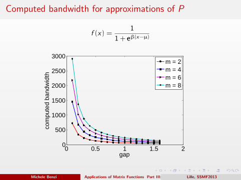
Computed bandwidth for approximations of P
f (x) =1
1 + eβ(x−µ)
0 0.5 1 1.5 20
500
1000
1500
2000
2500
3000
gap
com
pute
d ba
ndw
idth
m = 2m = 4m = 6m = 8
Michele Benzi Applications of Matrix Functions Part III: Quantum ChemistryLille, SSMF2013

Density matrix, Ne = 30, relative gap γ = 0.6
020
4060
80100
0
20
40
60
80
1000
0.2
0.4
0.6
0.8
1
Michele Benzi Applications of Matrix Functions Part III: Quantum ChemistryLille, SSMF2013

Density matrix, Ne = 30, relative gap γ = 0.2
020
4060
80100
0
20
40
60
80
1000
0.2
0.4
0.6
0.8
Michele Benzi Applications of Matrix Functions Part III: Quantum ChemistryLille, SSMF2013

Density matrix, Ne = 30, relative gap γ = 0.0001
020
4060
80100
0
20
40
60
80
1000
0.1
0.2
0.3
0.4
0.5
0.6
0.7
Michele Benzi Applications of Matrix Functions Part III: Quantum ChemistryLille, SSMF2013

Overview
1 The electronic structure problem
2 Density matrices
3 O(N) methods
4 A mathematical foundation for O(N) methods
5 O(N) approximation of functions of sparse matrices
6 A few numerical experiments
7 Some open problems
Michele Benzi Applications of Matrix Functions Part III: Quantum ChemistryLille, SSMF2013

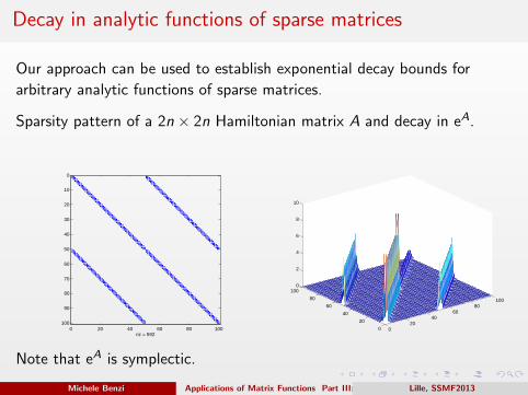
Decay in analytic functions of sparse matrices
Our approach can be used to establish exponential decay bounds for
arbitrary analytic functions of sparse matrices.
Sparsity pattern of a 2n × 2n Hamiltonian matrix A and decay in eA.
0 20 40 60 80 100
0
10
20
30
40
50
60
70
80
90
100
nz = 5920
2040
6080
100
0
20
40
60
80
1000
2
4
6
8
10
Note that eA is symplectic.
Michele Benzi Applications of Matrix Functions Part III: Quantum ChemistryLille, SSMF2013

Decay for logarithm of a sparse matrix
Sparsity pattern of H = mesh3e1 (from NASA) and decay in log(H).
0 50 100 150 200 250
0
50
100
150
200
250
nz = 1377
Here H is symmetric positive definite.
Michele Benzi Applications of Matrix Functions Part III: Quantum ChemistryLille, SSMF2013

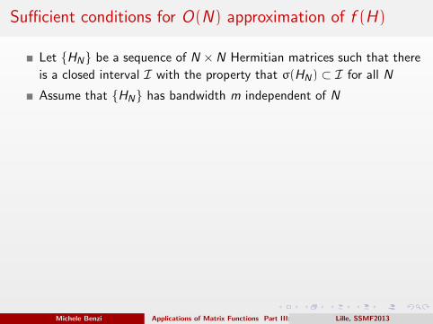
Sufficient conditions for O(N) approximation of f (H)
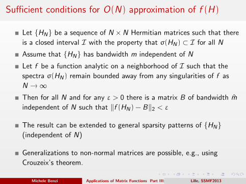
Let {HN} be a sequence of N ×N Hermitian matrices such that there
is a closed interval I with the property that σ(HN) ⊂ I for all N
Assume that {HN} has bandwidth m independent of N
Let f be a function analytic on a neighborhood of I such that the
spectra σ(HN) remain bounded away from any singularities of f as
N → ∞Then for all N and for any ε > 0 there is a matrix B of bandwidth m
independent of N such that ‖f (HN) − B‖2 < ε
The result can be extended to general sparsity patterns of {HN}(independent of N)
Generalizations to non-normal matrices are possible, e.g., using
Crouzeix’s theorem.
Michele Benzi Applications of Matrix Functions Part III: Quantum ChemistryLille, SSMF2013
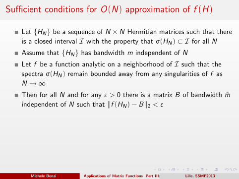
Sufficient conditions for O(N) approximation of f (H)
Let {HN} be a sequence of N ×N Hermitian matrices such that there
is a closed interval I with the property that σ(HN) ⊂ I for all N
Assume that {HN} has bandwidth m independent of N
Let f be a function analytic on a neighborhood of I such that the
spectra σ(HN) remain bounded away from any singularities of f as
N → ∞
Then for all N and for any ε > 0 there is a matrix B of bandwidth m
independent of N such that ‖f (HN) − B‖2 < ε
The result can be extended to general sparsity patterns of {HN}(independent of N)
Generalizations to non-normal matrices are possible, e.g., using
Crouzeix’s theorem.
Michele Benzi Applications of Matrix Functions Part III: Quantum ChemistryLille, SSMF2013
Sufficient conditions for O(N) approximation of f (H)
Let {HN} be a sequence of N ×N Hermitian matrices such that there
is a closed interval I with the property that σ(HN) ⊂ I for all N
Assume that {HN} has bandwidth m independent of N
Let f be a function analytic on a neighborhood of I such that the
spectra σ(HN) remain bounded away from any singularities of f as
N → ∞Then for all N and for any ε > 0 there is a matrix B of bandwidth m
independent of N such that ‖f (HN) − B‖2 < ε
The result can be extended to general sparsity patterns of {HN}(independent of N)
Generalizations to non-normal matrices are possible, e.g., using
Crouzeix’s theorem.
Michele Benzi Applications of Matrix Functions Part III: Quantum ChemistryLille, SSMF2013

Sufficient conditions for O(N) approximation of f (H)
Let {HN} be a sequence of N ×N Hermitian matrices such that there
is a closed interval I with the property that σ(HN) ⊂ I for all N
Assume that {HN} has bandwidth m independent of N
Let f be a function analytic on a neighborhood of I such that the
spectra σ(HN) remain bounded away from any singularities of f as
N → ∞Then for all N and for any ε > 0 there is a matrix B of bandwidth m
independent of N such that ‖f (HN) − B‖2 < ε
The result can be extended to general sparsity patterns of {HN}(independent of N)
Generalizations to non-normal matrices are possible, e.g., using
Crouzeix’s theorem.
Michele Benzi Applications of Matrix Functions Part III: Quantum ChemistryLille, SSMF2013
Overview
1 The electronic structure problem
2 Density matrices
3 O(N) methods
4 A mathematical foundation for O(N) methods
5 O(N) approximation of functions of sparse matrices
6 A few numerical experiments
7 Some open problems
Michele Benzi Applications of Matrix Functions Part III: Quantum ChemistryLille, SSMF2013
Approximation of f (H) by Chebyshev polynomials
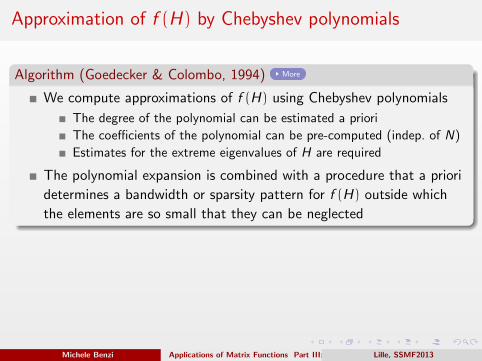
Algorithm (Goedecker & Colombo, 1994) More
We compute approximations of f (H) using Chebyshev polynomials
The degree of the polynomial can be estimated a priori
The coefficients of the polynomial can be pre-computed (indep. of N)
Estimates for the extreme eigenvalues of H are required
The polynomial expansion is combined with a procedure that a priori
determines a bandwidth or sparsity pattern for f (H) outside which
the elements are so small that they can be neglected
Cost
This method is multiplication-rich; the matrices are kept sparse
throughout the computation, hence O(N) arithmetic and storage
requirements. Matrix polynomials can be efficiently evaluated by the
Paterson-Stockmeyer algorithm.
Michele Benzi Applications of Matrix Functions Part III: Quantum ChemistryLille, SSMF2013

Approximation of f (H) by Chebyshev polynomials
Algorithm (Goedecker & Colombo, 1994) More
We compute approximations of f (H) using Chebyshev polynomials
The degree of the polynomial can be estimated a priori
The coefficients of the polynomial can be pre-computed (indep. of N)
Estimates for the extreme eigenvalues of H are required
The polynomial expansion is combined with a procedure that a priori
determines a bandwidth or sparsity pattern for f (H) outside which
the elements are so small that they can be neglected
Cost
This method is multiplication-rich; the matrices are kept sparse
throughout the computation, hence O(N) arithmetic and storage
requirements. Matrix polynomials can be efficiently evaluated by the
Paterson-Stockmeyer algorithm.
Michele Benzi Applications of Matrix Functions Part III: Quantum ChemistryLille, SSMF2013

Chebyshev expansion of Fermi-Dirac function
The bandwidth was computed prior to the calculation to be ≈ 20; here H
is tridiagonal (1D Anderson model).
Table: Results for f (x) = 11+e
(β(x−µ))
µ = 2, β = 2.13 µ = 0.5, β = 1.84
N error k m error k m
100 9e−06 18 20 6e−06 18 22
200 4e−06 19 20 9e−06 18 22
300 4e−06 19 20 5e−06 20 22
400 6e−06 19 20 8e−06 20 22
500 8e−06 19 20 8e−06 20 22
Michele Benzi Applications of Matrix Functions Part III: Quantum ChemistryLille, SSMF2013

Computation of Fermi-Dirac function
100 150 200 250 300 350 400 450 5000.5
1
1.5
2
2.5
3
3.5x 10
6
n
# of
ope
ratio
ns
mu = 2, beta = 2.13mu = 0.5, beta = 2.84
The O(N) behavior of Chebyshev’s approximation to the Fermi–Dirac
function f (H) = (exp(β(H − µI )) + I )−1.
Michele Benzi Applications of Matrix Functions Part III: Quantum ChemistryLille, SSMF2013
Chebyshev expansion of entropy-like function
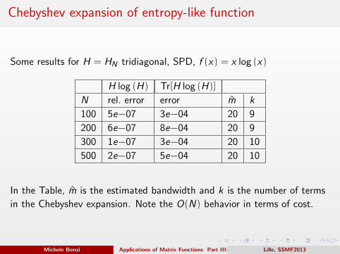
Some results for H = HN tridiagonal, SPD, f (x) = x log (x)
H log (H) Tr[H log (H)]
N rel. error error m k
100 5e−07 3e−04 20 9
200 6e−07 8e−04 20 9
300 1e−07 3e−04 20 10
500 2e−07 5e−04 20 10
In the Table, m is the estimated bandwidth and k is the number of terms
in the Chebyshev expansion. Note the O(N) behavior in terms of cost.
Michele Benzi Applications of Matrix Functions Part III: Quantum ChemistryLille, SSMF2013

Summary
‘Gapped’ systems, like insulators, exhibit strong localization
Localization in P = f (H), when strong enough, can lead to fast
approximation algorithms
Our decay bounds for density matrices depend only on the gap γ and
on the sparsity of H; they are, therefore, universal
These bounds can be useful in determining appropriate sparsity
patterns (or bandwidths) that capture the nonnegligible entries in
P = f (H)
Constants in O(N) algorithms can be large. In practice, to beat
O(Np) algorithms (p = 2, 3) on real problems, N must be large
enough.
Extensions to non-Hermitian case possible (applications??)
Michele Benzi Applications of Matrix Functions Part III: Quantum ChemistryLille, SSMF2013

Overview
1 The electronic structure problem
2 Density matrices
3 O(N) methods
4 A mathematical foundation for O(N) methods
5 O(N) approximation of functions of sparse matrices
6 A few numerical experiments
7 Some open problems
Michele Benzi Applications of Matrix Functions Part III: Quantum ChemistryLille, SSMF2013

Some open problems
The bounds represent the worst-case scenario and can be pessimistic.
To improve them, one must make use of additional information, such
as the eigenvalue distribution, which may not be readily available.
How to deal with metallic systems (γ → 0 as N → ∞)?
1 Wavelets?
2 H-matrices? Multipole methods? Domain Decomposition...?
3 Optimally localized bases? P = XX ∗, X = [u1, . . . , uN ]
What is the effect of errors in estimating λmin, λmax, and γ?
What about other asymptotics? E.g., scaling for C → ∞?
Which are the best O(N) algorithms? There are many of them...
An excellent introduction: C. Le Bris, Computational Chemistry from the
Perspective of Numerical Analysis, Acta Numerica 14 (2005), 363-444.
Michele Benzi Applications of Matrix Functions Part III: Quantum ChemistryLille, SSMF2013
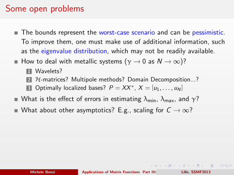
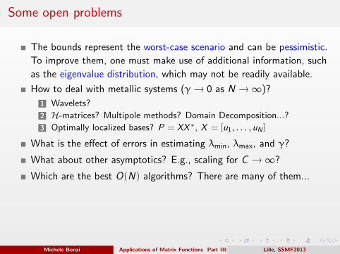
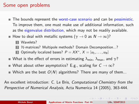
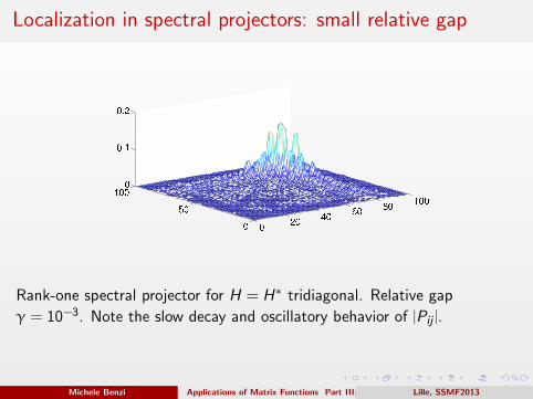
Localization in spectral projectors: small relative gap
Rank-one spectral projector for H = H∗ tridiagonal. Relative gap
γ = 10−3. Note the slow decay and oscillatory behavior of |Pij |.
Michele Benzi Applications of Matrix Functions Part III: Quantum ChemistryLille, SSMF2013

Localization in spectral projectors: large relative gap
Rank-one spectral projector for H = H∗ tridiagonal. Relative gap γ = 0.5.Back
Michele Benzi Applications of Matrix Functions Part III: Quantum ChemistryLille, SSMF2013

Chebyshev approximation
For H with σ(H) ⊂ [−1, 1] the Chebyshev polynomials are given by
Tk+1(H) = 2HTk(H) − Tk−1(H), T1(H) = H, T0(H) = I .
Then f (H) can be represented in a series of the form
f (H) =
∞∑k=0
ckTk(H).
The coefficients of the expansion are given by
ck ≈2
M
M∑j=1
f (cos(θj)) cos((k − 1)θj),
where θj = π(j − 12)/M. Back
Michele Benzi Applications of Matrix Functions Part III: Quantum ChemistryLille, SSMF2013

The N-independence of the error
The mth truncation error without dropping can be written as
‖em(H)‖ = ‖f (H) −
m∑k=0
ckTk(H)‖.
For x in [−1, 1] we have that |Tk(x)| ≤ 1 for k = 1, 2, . . . . Then
‖em(H)‖ = ‖∞∑
k=m+1
ckTk(H)‖ ≤∞∑
k=m+1
|ck |.
Back
Michele Benzi Applications of Matrix Functions Part III: Quantum ChemistryLille, SSMF2013

A Theorem of Bernstein
The set of Faber polynomials can be used to obtain a uniform
approximation to an analytic function f with a sequence of polynomials of
bounded degree, i.e.,
|f (z) − ΠN(z)| < cqN (0 < q < 1)
for all z ∈ F , where c and q depend on the analytic properties of f .
Example – Disk
If the region is a disk of radius ρ centered at z0, then for any function f
analytic on the disk of radius ρ/q centered at z0, where 0 < q < 1, there
exists a polynomial ΠN of degree at most N and a positive constant c
such that
|f (z) − ΠN(z)| < cqN ,
for all z ∈ F .
Back
Michele Benzi Applications of Matrix Functions Part III: Quantum ChemistryLille, SSMF2013
Top Related