Download - Annals of the University of North Carolina Wilmington ... · University of North Carolina Wilmington International Masters of Business ... (Bajaj, M. et al 2002) Company size: ...

Annals of the

University of North Carolina Wilmington

International Masters of Business Administration

http://csb.uncw.edu/imba/

http://www.csb.uncw.edu/imba/

AN EMPIRICAL EXAMINATION OF THE MARKETABILITY DISCOUNT ON CLOSELY HELD COMPANIES

Johannes von Olfers

A Thesis Submitted to the University of North Carolina Wilmington in Partial Fulfillment

of the Requirements for the Degree of Master of Business Administration

Cameron School of Business

University of North Carolina at Wilmington

2012

Approved by

Advisory Committee

Peter W. Schuhmann J. Edward Graham

Joseph A. Farinella

Chair

Accepted by

______________________________ Dean, Graduate School

ii

TABLE OF CONTENTS

TABLE OF CONTENTS ................................................................................................................................ii

ABSTRACT ................................................................................................................................................ iii

LIST OF TABLES ........................................................................................................................................ iv

INTRODUCTION ....................................................................................................................................... 1

LITERATURE REVIEW ............................................................................................................................... 3

Factors for Lack of Marketability ......................................................................................................... 3

Different techniques to estimate the marketability discount ............................................................. 5

Benchmark Method ......................................................................................................................... 5

Quantitative Marketability Discount Model ................................................................................... 5

Restricted Stock Studies .................................................................................................................. 6

Pre-IPO studies ................................................................................................................................ 7

Different Court Cases .......................................................................................................................... 8

The Mandelbaum Case .................................................................................................................... 8

The Johan Paul Mitchell Systems (“JPMS”) Case ........................................................................... 10

Peracchio Case ............................................................................................................................... 11

Selma K. Friedman Case ................................................................................................................ 13

RESEARCH QUESTION AND HYPOTHESIS............................................................................................... 15

DATA ...................................................................................................................................................... 16

METHODOLOGY ..................................................................................................................................... 17

TABLES ................................................................................................................................................... 22

REFERENCES .......................................................................................................................................... 30

APPENDIX .............................................................................................................................................. 30

iii

ABSTRACT

This paper measures the marketability discount for closely held companies and provides new

evidence regarding the size of this discount. The comparison of ratios between private and public

companies of a certain industry will estimate the discount. Although the ten factors of the

Mandelbaum case are the basis of this examination. Furthermore, the paper examines key variables

that impact the size of this discount. The result due to the data set of private and public transactions

in the last three years is a premium of 45,58%. The premium reflects the fact that an overall or

benchmark marketability discount with a few assumptions cannot perfectly predict a marketability

premium or discount.

iv

LIST OF TABLES

Table Page

1. Materials EV/EBITDA ....................................................................................................................... 22

2. The public benchmark EV/EBITDA ................................................................................................... 22

3. Weighted Premium/Discount .......................................................................................................... 23

4. Descriptive Statistics ........................................................................................................................ 24

5. Correlation Coefficients ................................................................................................................... 25

6. Regression Analysis ......................................................................................................................... 26

7. H2: Multiple Regressions: Dependent Variable Discount/Premium ................................................ 27

8. H3: Multiple Regressions: Dependent Variable Discount/Premium ................................................ 27

9. H4, H5,: Simple Regressions: Dependent Variable Discount/Premium ............................................ 28

10. H6: Multiple Regressions: Dependent Variable Discount/Premium .............................................. 29

INTRODUCTION

One of the key differences between public and privately traded companies is the marketability

or liquidity. It is an indicator of how easy respectively owned shares or companies can be sold

quickly, with minimal transaction cost or minimal price concessions. This paper focuses on the

marketability discount for closely held companies.

The sale of listed shares is a simple implementation. Between contacting the broker and the

final sale of the share normally takes a minute or even a few seconds. On the other hand selling a

closely held company or shares with a non-existing market, is a difficult process. The most difficult

part is to indicate the fair market value of a private company because the key data of private

translated companies are mostly not published. There are three accepted methods to calculate the

fair value of a closely held company: the income approach, the asset approach and the market

approach. After an investor arrives at a fair value of a closely held company they must then adjust

that value for a marketability discount and a minority shareholder discount. The fair value minus

these two discounts results in a fair market value of the firm. The existing literature indicates that

this value ranges from 5% - 50%. This paper examines the magnitude of the marketability discount

and provides new evidence regarding the size of this discount. The paper also examines key

variables that impact the size of this discount.

It is very difficult to examine the marketability discount since data on closely held companies is

not readily available. It is also nearly impossible, to find a set of comparable private transactions

which has the same company parameters like sales or earnings in a similar industry.

The discount mostly reflects the lack of liquidity. The discount could include transaction cost,

lack of marketability or minority interest. The discount for minority interest or especially for lack of

marketability is placed at the end of many private company valuations. The transaction costs are

mostly included in one of the discounts and not listed separate. The minority discount reflects an

2

investment stake of a company less than 50%. This paper focuses on the discount for lack of

marketability. In the business world, a discount for lack of marketability, as mentioned above, is

applied to privately held companies, especially companies which are not traded regularly.

Marketability discount considers the expected higher financial and time expenses etc. (Koeplin et

al,2000).

Some valuation approaches like the income approach already include some kind of “discount for

lack of marketability” in their valuation process. In that case it is called market risk. The Capital Asset

Pricing Model (CAPM) is a component of the cost of capital used in the income approach.

Furthermore the cost of capital is a function of beta and beta is a multiple for the market risk. One

could imagine that the discount for illiquidity could be subtracted twice, once in the market risk and

secondly in the discount for lack of marketability. The beta shows the level of systematic risk in a

particular asset, relative to the average. Therefore it doesn´t reflect a specific uncertainty of the

market related to a private held company.

A discount for a closely held company is a non-fixed figure which has changed over the last

decades. Still many private company valuations contain a fixed illiquidity discount or discount rate.

These fixed discounts are related to handbooks or former court cases which have discussed private

company valuations.(Damodaran, 2005). Before determining an actual discount it is advisable to

understand the movement of the discount during the last years.

According to research using restricted stocks and pre-IPO prices the average discount for private

firms between 1999 and 2006 was 20%-25%. (Block, 2002). Lance S. Hall (2011) illustrates, due to the

benchmark method an average discount of 35% during 1980 and 1996. In previous years, it was

common in business valuations to use a 35% marketability discount for all closely held firms. Today

the U.S Tax Court does not except any kind of “standardized” discount. Consequently, the court asks

a business appraiser to justify his or her discount and consider the companies; financial risk,

management, dividend policy, industry, business risk, revenue and assets. This leads to a range of

3

marketability discounts for closely held firms. (Paschall, 2005). The marketability discounts tend to

fall into the 15% - 25% range.

The goal of this paper is to measure the marketability discount for closely held companies. The

method to indicate the discount will be based on transaction data of German, UK, and US private

companies. Finally, the comparison of ratios between private and public companies of a certain

industry will estimate the discount. Another goal is to indicate the factors of the discount size.

Factors could be a function of size, industry, profit, type of assets or region for example. A multiple

regression of the transaction data will find and indicate the impact of the factors. In the literature

review many factors will be summarized which have impacted the discount for lack of marketability

in the past. It will be interesting to figure out if factors like financial risk have a bigger impact at the

discount then company size.

LITERATURE REVIEW

The literature review part of this paper is very important. This part includes factors for lack of

marketability, different approaches to indicate the marketability discount and court cases of the

marketability discount which have been discussed and caused a stir in the past. Due to the

difficulties, experiences and assumptions of the cases it might help to figure out a new approach or

would improve an already existing approach with new assumptions.

Factors for Lack of Marketability

The explanation of some factors for lack of marketability will define the higher financial and

time expenses.

Availability and accessibility of corporate information:

A restriction in obtaining information of corporates increases the uncertainty and therefore

influences the marketability. (Cheridito, Y. et al 2008). The case of uncertainty, regarding the asset´s

4

value for example, will increase the discounts claimed by investors. Uncertainty for investors is

consistent with risk, thus expensive for the owner. (Bajaj, M. et al 2002)

Company size:

A company size is an important indicator for the size of the discount. A big and profitable

company entails mostly larger sales and larger net income etc. compared to smaller firms. Therefore

larger companies tend to have a smaller discount. More liquidity is the key factor of this statement.

(Block, 2007)

Control Component:

A stake of a private company smaller than 50% is less-attractive investment. Less-attractive

investment reflects a big discount, due to illiquidity. More than 50% on the hand is more liquid and

therefore more expensive. (Damodaran, 2005).

Attractiveness of the industry environment:

Condition and future prospects of the industry, the amount of possible acquirer and

competitive situation could have a high and important influence on a company’s marketability.

(Cheridito et al, 2008)

Duration of restrictions on trade:

The longer a company is on the market for sale, the greater is the loss of value and the

stronger the lack of potential buyers. The long duration shows interested investors the non-

marketability of an asset, otherwise the asset would be sold straight after being on the trade market.

Dropping the value of an asset by increasing its marketability discount, will gain new investors as

buyers or shareholders. (Bajaj, M. et al 2002)

5

Modification to Rule 144A

Rule 144 was implemented in 1934 by the Securities and Exchange Commission (SEC) which

states that unregistered securities have a holding period of two years. The holding period was

implemented to recover shares from underwriting or distribution. (SEC 2008). In 1990 the SEC

modified the rule to 144A. The differences are that the holding period dropped from two to one year

and that qualified institutional investors got the provision to deal with unrestricted stocks without

the registration certification between each other. In 2008 the holding period, according to SEC, fell

further to six months. Due to the shorter holding period the securities got more liquid and the

marketability discount increased since the modification.(Duane Morris 2008)

Different techniques to estimate the marketability discount

Not only factors can influence the marketability discount. To indicate the right marketability

discount, the right approach can help and cause significant size differences. It always depends on the

information which is available to find the right approach and therefore to define the appropriate

discount. It is important to understand the differences between the methods.

Benchmark Method

The most famous method is the benchmark method. The difference between a publicly

traded stock and an identical restricted stock is the basis of the calculation. Based on the differences

of many transactions, the average is used as a measure of the marketability discount. The courts

criticized this approach, stating that an average does not compare directly with a specific data. (Hall,

2011)

Quantitative Marketability Discount Model

The benchmark discount doesn´t consider the wide range of different investment

characteristics between a privately held company and a public traded company. Therefore the

6

marketability discount should reflect more the economic characteristics of an asset. Due to the five

assumptions of the Quantitative Marketability Discount Model (QMDM), a determination of the

marketability discount, under consideration of the economic characteristics, is conceivable. The first

factor to consider is the expected growth in value. In case of an illiquid security the growth will be

the future value which an investor estimates to achieve. Next the quantification of expected

dividends or distributions of the asset has to be incorporated. That is one of the differences between

the QMDM and the benchmark analysis. A qualitative comparison of dividends with another

investment is not possible. The third factor to take under consideration is the expected growth in

dividends or distributions. In this case assumptions are adequate because the growth of an illiquid

security may not be that large. The expected holding period for an investment is the fourth factor.

That is one of the criticisms of the QMDM because it is impossible to indicate the holding period for

an illiquid security. The last factor is the required return. The equation is not relevant for this paper,

because as shown under the first four factors the QMDM will not be used for further calculation. The

positive aspects of this model are the assumptions but which are on the other hand not really

reasonable. (Mercer, 2003)

Restricted Stock Studies

The Restricted Stock Studies, which will be defined next, is the most preferred approach of

the Courts. This study has been cited and analyzed by many court decisions. The basic of this

approach is quite similar to the benchmark method. As well, the evidence of the marketability

discount is the price difference between a restricted private placement and its publicly traded twin.

The key of the approach is the comparative analysis. The discount of the Benchmark Method consists

of the average of many comparisons, as explained above. Regarding the Restricted Stock Studies the

appraiser compares factors like market value, revenue or profitability of the private asset with the

public asset. Therefore this approach is more liable then others because the comparison takes only

place with companies which have similar factors. (Block, 2007)

7

Three different approaches have been derived from the Restricted Stock Studies and partly

accepted by Courts. They are called the Bajaj Method, the Burns Method and the FMV Method. The

explanation of these three methods in this paper will only contain the important difference to the

Registered Stock studies and will not be pointed out deeply. The Bajaj Method focuses on the

comparison of private stocks that are discounted registered and unregistered. In the opinion of the

Bajaj Method there must be other reasons than lack of marketability for private companies selling

registered stocks at discount because they could reach the price of the public market. Regarding the

Bajaj data, the marketability discount should be under 10 %. (Bajaj et al, 2002). Mr. Burns argued

that the marketability discount should be defined into two different parts. One part is the holding

period which has changed after the modification of Rule 144 and the second part is market access.

Due to Rule 144a a registered stock is more liquid thanks to the shorter holding period. Therefore

Mr. Burns indicates that the discount should be lower since 1990. Also he makes the difficult market

access for restricted stocks before 1990 responsible for the higher discounts. (Hall, 2011). FMV

Opinions, Inc. has carried out a study to find the right marketability discount. Therefore they

researched 230 transactions from 1980 to April 1997. The result of the overall study was called FMV

Restricted Stock Study. They indicated an average discount of 22.3% for all 230 transactions. One

important result of this study is the percentage block size. Due to the information it can be shown

that the discount of big block sizes is 10-15 percent higher than for small block sizes. A reason for this

statement is probably the longer holding period of big block sizes due to the Rule dribble-out

provision.

Pre-IPO studies

The last approach of this paper is called Pre-IPO studies. This approach is a qualified

alternative to the restricted stock studies. The price difference of a stock listed as initial public

offerings (IPOs) and a stock price of the same company, prior going public, is the indicator for the

8

marketability discount. Based on the following study of Pratt (Pratt, 2001) the mean discounts can

verify between 42 % and 60 % which is quite a lot.

The uncertainty of this approach is recorded very well in the table above. Primary the holding period

of a pre-IPO share cannot be set and is therefore critical for investors. It is not even determinate that

the shares will be transferred into the publicly traded market. In the time gap between 1995 and

1997 only 91 of 732 transactions into IPOs took place. Due to the uncertainty the price of prior IPOs

are too low and the marketability discount too high. Moreover, only information of successful

companies are useful for this approach. Another factor for the uncertainty is the financial structure

of a company which might change during the years of going public. (IRS, 2009)

Different Court Cases

The following Court Cases show how the marketability discount can influence the company

value of private companies.

The Mandelbaum Case

Until 1976 three Mandelbaum brothers, who had founded the company Big M, Inc., were all

equal shareholders. From 1976 the Mandelbaum brothers started to transfer shares to their children.

Big M had retail stores along the north and central eastern coast and distributed woman´s apparel.

Due to the shareholders´ agreement no specific transfer value of the corporation was set. When

1990 it came to the gift tax return preparation, the freely-traded values of the stock were stipulated

at trial, as usual. “A shareholders´ agreement was in effect, providing the corporation with the right

of first refusal”. This agreement had an important role in the courts decision later on. However the

discount for lack of marketability was committed by family´s experts to 70 % and of the IRS experts

to 30 %. Information of other investors were collected by the family experts to underline their

decision. As well they considered a holding period of 10 to 20 years because this would be the

retiring period of the next generation. The Restricted stock studies and the IPO studies were the basis

9

of their assumptions. Both were referring to different cases with a median discount of 33 % due to

the restricted stock studies and 45% regarding the IPO studies.

The Court stated the following factors should be considered for the proper marketability

discount. The first factor to consider is “private vs. public sales of stocks”, which examines the sales

of similar companies and their marketability´s. Next, an analysis of financial statements must be

conducted to determine the viability of the firm. The third factor to take under consideration is the

company´s dividend policy because this helps to determine if the investor will receive a return on his

investment. Thus a company that does not pay dividends will have less marketability. Fourth, the

marketability discount must attempt to capture the nature of the company, i.e. that firm´s reputation

and their position in their specific market, as well as their economic outlook. Executive management

is the driving force behind a company, therefore management should be taken under consideration

as well. A strong management team can have a positive influence on a company´s value. Moreover,

the amount of control that shareholders have over a company is a factor to consider. The more

control a shareholder has over a company can increase that value of a company, or in this case,

decrease the marketability discount. The seventh factor to consider is the existence of any restriction

on the ability of a shareholder to transfer shares of a company. If there are legal roadblocks that

hinder the ability of a shareholder to transfer stock, then the value of a company will be reduced.

Additionally, the value of a company must be reduced if an investor must hold onto his shares of the

company for an extended period of time before he can sell his shares and realize a gain. Companies

that have a redemption policy, the company´s right to purchase stock before it is sold to an outsider

is also a contributing factor to the marketability discount, because it is common that embedded in a

redemption policy is a set price at which the shares must be sold. Finally, the last factor that must be

considered is the cost that would be associated with taking the company public. The marketability

discount will increase, if the investor must bear the entire cost of registering a private stock. The

court concluded, due to the ten factors, a marketability discount of 30 %. The court didn´t accept the

10-20 years holding period and indicated that the family experts shouldn´t only interview venture

10

capitalists or LBO groups because this kind of investor always want to beat down the prices. (Hawkins

et al, 2003)

The Johan Paul Mitchell Systems (“JPMS”) Case

In 1989 the co-founder of the hair-care products company JPMS Paul Mitchell died. He had a

minority interest of 49.04 % shares. “On July 21, 1993 the IRS informed the Estate of Paul Mitchell

(“Estate”) the deficiency in the federal estate tax in the amount of $45,177,089, and a total of

$8,543,643 in penalties”. The accusation of the IRS was that the private accounting firm of the Estate

had undervalued the 1,226 shares of JPMS stock. Due to the valuation of the Estate, the stocks had a

value of $ 28.5 million and based on the calculations of the IRS the value was $ 105 million. It

amounted to a $76.5 million difference of additional tax, which was assessed by IRS. Also the IRS

accused the Estate of a delay in tax return. This accusation will not be discussed. Only the difference

of the stock value is interesting for this paper. Finally the differences of the stock value proceeded to

trial. The experts of the Estate indicated a value for the 1,226 stocks of approximately $20 to $29

million, while the IRS a range of $57 to $165 million. The approach to calculate the value was nearly

the same with both experts, they compared the stock price of similar companies. “Basically the

Estate indicated that the reputation of the company suffered after John Paul`s death, costs of

litigation between the Estate and the co-founder of Paul Mitchell, cash-flow patterns, the

competition in the hair- care industry and the marketability of the Estate´s minority”. (Hawkins et al

2001).

Due to the research of the Tax Court in 1997 they defined a stock´s fair market value of

$41,532,600. The court weighted their statement under the following assumptions. First the court

assigned a value of $ 150 million which was worth the offer from Gillette, Co. for the company. Then

they decreased the value by 10 % for the loss of presence and creativity of Mr. Mitchell. Secondly

they calculated the 49.04 % shares of the state, minus a 35 % discount for lack of marketability

combined with minority interest. Finally a subtraction of $1.5 million of possible lawsuit against the

11

co-founder. In November 1997, the estate argued that the discount for minority interest and lack of

marketability should at least be 45 % due to the expert witness George Weiksner. Even the second

motion in July 8, 1998 for reconsideration was rejected by the Tax court. The estate asked for more

detailed explanations how it figured out the combined discount. The court replied that “valuation is

necessarily an approximation and a matter of judgment, rather than one of mathematics, on which

petitioner has the burden of proof”.(Hawkins et al 2001).

The tax court made a typical announcement by shifting the burden of proof on the Estate.

They didn´t even explain their combined discount. It looked like they used the discount because it

was like this in the past, without actual research. Another problem could be that they didn´t

distinguish between the marketability discount and the discount for minority interest. Instead they

used a combined discount. Due to the Commissioner´s expert, Hanan, she calculated with a 30 %

marketability discount and a minority discount of 23.1 % showing combined discount of 46.2 %. The

estate´s expert, Weiksner, on the other hand defined his marketability discount with 45% and the

minority discount with 30% and his final combined discount was 61.5 %. Regarding the two

calculations it is obvious that the combined discount of the tax court was only in the range of the

expert’s marketability discount alone.

Peracchio Case

Peter S. Peracchio, the petitioner, in due time filed a petition for redetermination. Due to the

Judge he has a deficiency in Federal gift Tax for the Year 1997 of $328,317. Regarding many different

transfers of partnership units the discount for lack of control is an important factor in this case. As in

the cases before the determination of the fair market value is the basic goal. What makes this case

different is the change of property between the family members and the family organization. Again

this case refers to a combined discount. The combination of lack of marketability and lack of control

reflects the discount. The petitioner had sold interest and therefore applied a combined discount of

40 %. The respondent contends a combined discount of 18.74 %. (Hawkins et al 2003).

12

Both parties confirmed a second discount after using the minority interest discount, which

would consider the lack of marketability. The petitioner´s experts, named Dr. Dankoff and Mr.

Stryker, analyzed the range of discount with the benchmark, restricted stock studies as basics and

finally determined the discount due to the factors of the Mandelbaum case. Mr. Dankoff stated in his

analysis that he reviewed the factors which relate to the subject partnership of the Mandelbaum

case. Also he analyzed other empirical studies and came to a range of 35% to 45% for the

marketability discount. Mr. Stryker states a 40 % discount was applicable. He focused on restricted

stock studies and stated that a discount around 30 % would be reasonable. The difference of the

additional 10%, he argued, relates to the fact that the Peracchio´s interests are freely traded, not like

the ones of the restricted stock studies. Furthermore he used average discount of all the different

cases he observed. The problem of Mr. Stryker´s analysis is that he didn´t implement any analytical

research, he totally relied on previous restricted stock studies. Another disadvantage of his analysis is

that he missed in his benchmark any reliable cases which focused on transferred interests. (Hawkins

et al 2003).

Mr. Burns the expert of the respondent offered another interesting “analysis”. In his opinion

a discount for lack of marketability discount should be in the range of 5% to 25%. He defines a higher

discount would be trivial and writes in his report due to a “conservatively-managed partnership

holding highly liquid marketable securities and cash investments.” As well he denies a discount below

5 % because the 5% would include the costs to find a willing buyer. He argued at court that the 5 %

limit would be charged by brokers as sales commission. Finally he announced a discount of 15%.

Among other things he defended his additional 10% as a discount for the thin nature of the

secondary market. (Hawkins et al 2003).

Banister Financial, Inc. analyzed the case and declared a marketability discount up to 25 % to

be appropriate. Especially the midpoint range of 15% of Mr. Burns was not accepted as a serious

discount announcement. Although they supported Mr. Burns statement that a more than 25%

13

discount for an entity with the characteristics of the partnership would be overvalued. They accused

the petitioners experts of lack of proof.

Selma K. Friedman Case

The petitioners of this case are the minority stockholders. They owned stocks of nine family

owned corporations. Each petitioner “had its dole asset a parcel of income-producing office,

commercial or residential real estate”. During a voting in 1986 the board of directors and the

majority stockholders decided to form a new partnership and therefore transfer all of the

corporations’ property. Petitioners did not approve and voted their shares against the transfers.

Later the corporation failed to announce a fair value of the petitioners stocks and a judicial

determination followed. The valuation occurred in two steps. In the first step the Supreme Court

calculated the net value of the leasehold interest of one office building owned by the corporation.

Then they summarized all nine net assets values. In the second step of the trial they declared the fair

value of all petitioners shares at the sight of the previously fixed net asset values. The petitioners’

experts preferred a fractional corporate stock ownership of the aggregate corporate net asset values.

It was rejected by Supreme Court because “valued these shares as if petitioners were co-tenants in

the real estate rather than corporate shareholders” and the lack of marketability would be

intercepted. Kenneth McGraw was the expert of the corporation and preferred by the court. He

finally determined the net asset value due to the hypothetical value of the assets. The illiquidity of

the shares for potential investors, regarding the fact that the shares of close corporations cannot be

changed immediately into cash, will be replaced by a discount. The corporation expert announced a

discount of 30.4% for unmarketability. The court considered that the discount includes a discount for

minority interest and subtracted 9.4%. Finally the Supreme Court applied a 21 % discount for lack of

marketability against each petitioners´ share interest of the total corporations´ net asset value.

The Supreme Court only relied on the two-step valuation approach of Mr. McGraw. In the

first step he took a discount of 9.8% which the court added back under the explanation that it would

14

reflect a minority discount. In the second McGraw implemented a discount of 30.4 for lack of

marketability and the court added back again the minority discount. Therefore the Court added back

twice the discount for minority, in every step once. The court defended their preceding example due

to the fact that McGraw compared his discount “with restrictive sale provisions and *McGRaw+ found

that they exhibited a median discount of 30.4 % relative to net asset value”. Also the Supreme Court

stated that the analytical data of McGraw were based on minority shares and therefore his

unmarketability discount already included a minority status. McGraw defended himself and noted

that he actually calculated the discount for lack of marketability by comparing the purchase price of a

restricted stock with a public traded share. The public shares had the same features like minority and

fit to comparative corporations. In addition he compared share prices of minority and marketable

stocks with minority and unmarketable stocks. Therefore he did not contain any discounts for

minority. Finally the discount consists of the price differences of the two share classes. Due to the

fact the Supreme Court removed a nonexistent minority discount and so overvalued the shares.

In summary, the court cases listed above all have something in common, the courts didn´t

except the counterparty’s experts’ valuation decision and mostly reduced the discount for lack of

marketability. This occurred due to the fact that the counterparties mostly tried to undervalue their

companies to save taxes. The Friedman case is an exception. In that case the reasons are the

different valuation methods between the minority and majority stakeholders. The courts decisions

often base at discounts of the past which are already outdated. The courts announcement from the

Mandelbaum case on the other hand was exemplary. They explained their own decision based at

their own research and assumptions. These ten factors were and still are used for court decisions.

During the court cases above, the discount for marketability and minority interest were often mixed

up. These discounts have to be presented independent. They are not highly related to each other and

often caused misunderstandings.

15

RESEARCH QUESTION AND HYPOTHESIS

The court in the Mandelbaum case recommends that analysts and researchers examine the sale

of private and public stocks to estimate the marketability discount and this is the motivation of this

paper. Due to the research above, most courts used an overall discount that did not vary in different

industries. The examination of the discount size and the factors that influence the discount is another

motivation of this paper. Based on the court decisions of the Madelbaum case (Hawkins et al, 2003)

and the restricted stock studies (Block, 2007) the following hypothesis will be verified:

H1: Are marketability discounts for private companies higher than 25%?

H2: Do marketability discounts for private companies vary across countries?

H3: Do marketability discounts vary over time?

H4: Do marketability discounts for private companies vary with size?

H5: Do marketability discounts vary with financial risk?

H6: Do marketability discounts vary between different industries?

16

DATA

The origin of the Data is Capital IQ. The Capital IQ database provides data about company

transactions and is a Standard & Poor´s Business.(www.capitaliq.com). The currency of the Data is

the EUR and all figures in the dataset are set at announcement.

To verify the hypothesis, this data takes into consideration companies in Germany, United

Kingdom and United States and Canada. The United States and Canada are, due to the database, only

on area and cannot be classified independent.

The time horizon reflects the duration from January 22nd 2009 until November 21st 2011. The

time horizon makes it possible to indicate a discount which is up to date.

This paper will define the marketability discounts of different primary sectors. They are

Industrials, Materials, Energy, Information Technology, Utilities and Healthcare.

To verify the marketability discount, datasets from private and public companies are necessary.

This dataset reflects in total 238 observations. 91 observations of private companies and 147

observations of public companies will be the basis.

The dataset consists of M & A in the last two years. Not every transaction reflects a 100 percent

M & A. It has to take into consideration that it is difficult to find data from private transactions.

Therefore this dataset as well includes transactions of company shares. As mentioned in the court

cases above, sales of minority or majority interests are often basis of court decisions.

Hardly every transaction in this dataset lists the classification figures Transaction Value, Revenue

and total Assets. These figures will support the research for factors of the marketability discount.

http://www.capitaliq.com/

17

METHODOLOGY

The data set contains transactions of private and public companies. This data is necessary to

solve the first hypothesis whether the actual marketability discount is higher than 25%. First the price

multiples EV/EBITDA for each transaction will be calculated. To obtain a discount or premium I will

compare the EV/EBITDA of private and public transactions. For the comparison I calculated an

average public EV/EBITDA of every industry and region as seen in the following table. Every multiple

of each industry sector and region will be added and divided by its number, to get a specific industry

average. To get more observations I implemented the region Europe. Therefore the regions

USA/Canada and Europe are the assumptions. One example of the average EV/EBITDA materials

industry can be seen in table 1.

The different industries averages of this paper contain industrials, materials, energy,

information technology, utilities and healthcare. Finally to calculate the discount or premium the

EV/EBITDA of a private transaction will be subtracted from the public industry average and the result

will be divided by the public industry average.

The following model will be used to calculate the discount:

DT(x) =

DT(x) = Transaction discount

pt= private transaction

ia= Industry average

The average of all private transactions discounts or premiums of a particular industry will be

the industry marketability discount or premium. Finally I added the weighted industry discounts or

premium to get the overall Marketability discount. I weighted the industry discount because not

every industry has the same amount of transactions.

18

D= IDT(x1)*mean(x1)+ IDT(x2)*mean(x2)+ IDT(x3)*mean(x3)……………………….

IDT(x) = Industry marketability discount or premium

D= Marketability Discount

Hypothesis two to six will be defined by a multi regression model. First of all the correlation

coefficients of the variables will show us a first small overview and might show us in which direction

the marketability discounts tend to orientate. The variables of the hypothesis will be replaced by the

following data figures:

H2: country = the different countries will be replaced by dummy variables

H3 : time = Time 2011= 1 if 2011, 0 otherwise;

Time 2010= 1 if 2010, 0 otherwise;

Time 2009= 1 if 2009, 0 otherwise;

H4 : size = revenue

H5 : financial risk = D/E ratio

H6 : industries = the different industries will be replaced by dummy variables.

In the regression the premium or discount of each transaction will become the dependent

variable and the independent variables will be revenue, announcement date, D/E ratio and the three

different dummy variables which reflect the different industries.

Discount = β0 + β1X1 + β2X2 + β3X3 + β4X4 + β5X5

X1 = Country

X2 = Time

X3 = Revenue

X4 = D/E ratio

19

X5 = Industry

Simple regressions will get a more decent understanding of the effect of each independent

variable on the dependent variable and will avoid multicollinearity. This will help to clarify which

variable interacts the most the discount or premium.

DISCUSSION AND RESULTS

The public benchmark EV/EBITDA figures which I have used to calculate the discount or

premium can be seen in table 2. The first hypothesis proves whether the marketability discount of

private transactions is higher than 25%. Due to my transaction data and the equation above I

calculated an overall premium of 45.58%. This result occurs due to the different industries and

regions. The industry premiums or discounts of table 3 are the basis of the premium.

The companies in the healthcare sector for example have been sold at a premium of 152% and

the Information Technology companies on the other hand at a discount of 5%. The calculation is

connected to the first factor of the Mandelbaum case which states “Private vs. public sales of the

stock”. The different premiums or discounts support the fourth factor of the Mandelbaum case

which focuses on the nature of a company, position in the industry and the economic outlook. The

only sector with transactions of premiums is the healthcare industry. In all other industries the

companies have been sold nearly 50% at premium and nearly 50% at discount. It shows even if the

average of an industry has been sold at premium there are still many companies in that industry

which are not that liquid. The valuation of discounts or premiums in one industry reflects the second

factor of the Mandelbaum case. Different financial statements are the solution of the valuation.

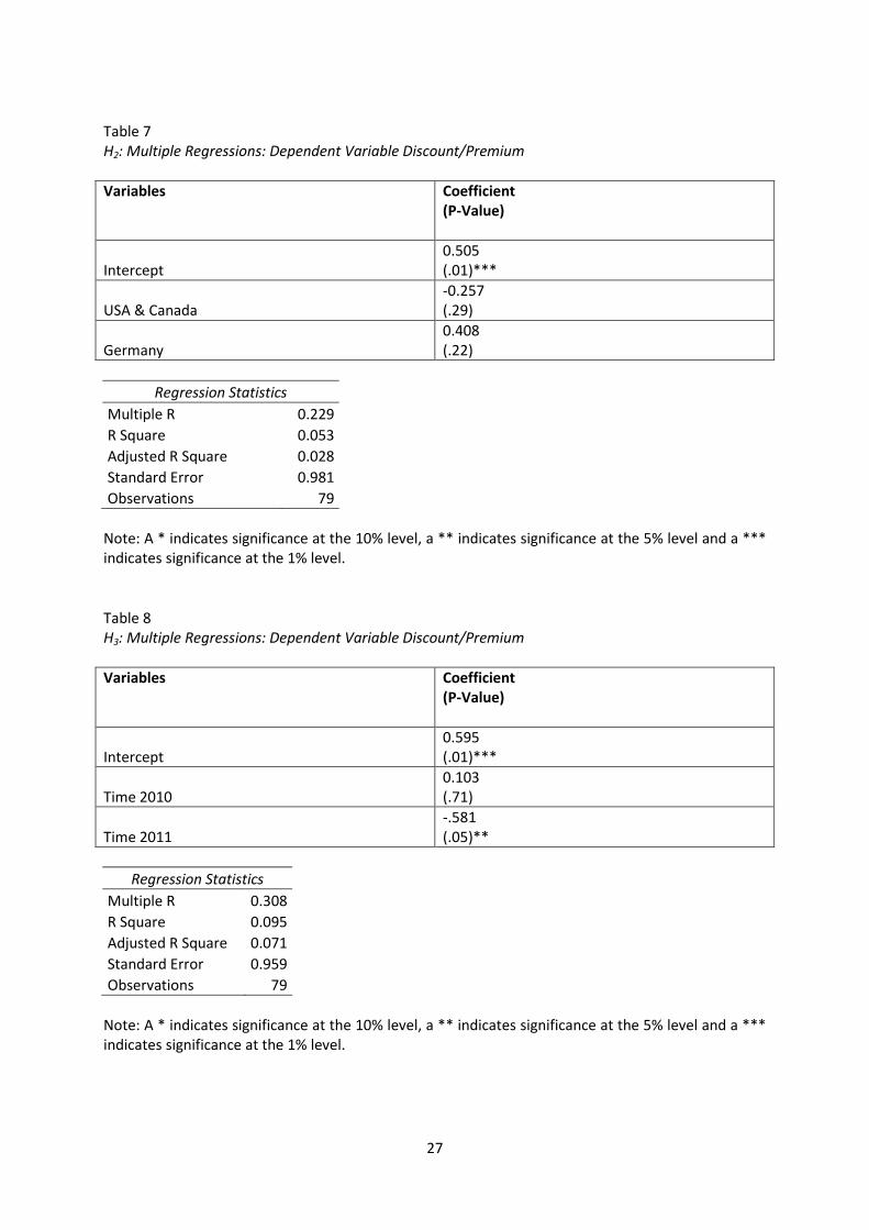
Table 4 shows the independent variables USA & Canada and Germany as well as the dummy

variable UK. The small adjusted R squared suggests that the regions do not perfectly fit to the

premium. USA & Canada show a very low significant level. Germany on the other hand shows more

20

significance. Regarding the low significance, it is difficult to find any relationship between the

premium and an area. The course of the low significant level is the small amount of observations. To

find a high level of significance in the USA & Canada region would be really difficult. A big n could

only reflect the huge USA & Canada area.

Even, the financial crises in 2008 couldn´t affect the average premium due to my data set. Only

the year 2011 indicates significance at the 5% level. The reason for the high level of significance could

be that most transactions have been from the USA & Canada area.

Table 6 includes the simple regressions of revenue and the d/e ratio with the premium or

discount as the dependent variable. Revenue shows the highest level of significance. It supports the

factor that big companies with high revenues have a smaller discount then smaller companies. The

second factor of the Mandelbaum case indicates to research the viability of a company. Furthermore,

table 6 shows that the d/e ratio has as well impact on the premium or discount and influences the

result.

Table 7 shows the independent industry variables with the information technology dummy

variable. This multiple regression has the highest adjusted r square. The healthcare industry shows

the highest level of significance of 99% and the utility industry of 95%. The reason is that all

transactions in the healthcare industry have been sold at premium. It reflects factor 4 of the

Mandelbaum case. The nature of the company is the industry sector. The industries with the smallest

premium or even discount have the lowest level of significance. It shows that the premium vary with

different industries. Therefore an overall or benchmark marketability discount with a few

assumptions cannot perfectly predict a marketability premium or discount.

21

CONCLUSION

This study intended to examine what size of a discount should be placed on privately held

companies. Due to the data set of private and public transactions in the last three years the result is a

premium of 46%. The premium reflects the fact that an overall or benchmark marketability discount

with a few assumptions cannot perfectly predict a marketability premium or discount.

The basis of this study was the Mandelbaum case with its ten assumptions. I didn´t use the

factors related to the comparison of restricted stocks. Therefore some factors were invalid. The

outcome underlines the approach of the Mandelbaum case to search for related company

characteristic features of public companies. Table 7 perfectly shows that related facts like the same

industry have a big input to investigate the right marketability discount or premium. Furthermore,

table 6 reflects that revenue shouldn´t be a rooter for a company valuation. The debt to equity ratio

on the other hand, is a good assumption for the company’s nature. It shows that the financial risk

influences the discount or premium.

The question of this thesis perfectly originated the problem of benchmark discounts or

premiums. Private companies in the information technology industry have been transacted at a

discount of 5% and in the healthcare industry on the other hand at a premium of 152%. A company

nature as well includes the place of origin. Transnational discounts or premiums shouldn´t be placed

as seen in table 4. As shown in the Europe region, it is related to the discount or premium.

The outcome of this study should show every appraiser or court, not to use a benchmark or

trend marketability discount. The ten factors of the Mandelbaum court case lead into the right

direction to valuate a marketability discount or premium. Every technique to estimate the

marketability discount can be a support but at the end the appraiser has to implement his own

assumptions and experiences. The setting of a marketability discount or premium should take more

time than just to use some benchmark discounts. Finally the right marketability discount or premium,

basing on the court cases, can save all interested parties a lot of money and time in court.

22

TABLES

Table 1 Materials EV/EBITDA

Date Country Company Status Industry EV/EBITDA

05/17/2011 Germany Public Company Materials 13.31



02/08/2010 Switzerland Public Company Materials 16.06

11/02/2009 Switzerland Public Company Materials 4.21




Average 9.21

Table 2 The public benchmark EV/EBITDA

Variables Energy Healthcare Industrials IT Materials Utilities

USA & Canada 10.76 9.34 9.2 25.74 15.22 8.94

Europe 7.96 9.72 9.92 23.71 9.21 8.34

23

Table 3 Weighted Premium/Discount

Industry Premium/Discount Mean Weighted

Premium/Discount

Energy 25% 0.228 5.70%

Industrials 17% 0.127 2.16%

Materials 40% 0.114 4.56%

Utilities 51% 0.177 9.03%

Healthcare 152% 0.165 25.08%

IT -5% 0.189 -0.95%

Total 45,58%

24

Table 4 Descriptive Statistics

Variables N Mean Median Min Max SD

Discount/ Premium 79 0.456 0.287 -0.775 3.832 0.995

Time 2010 79 0.443 0 0 1 0.500

Time 2011 79 0.316 0 0 1 0.468

USA & Canada 79 0.430 0 0 1 0.498

Germany 79 0.152 0 0 1 0.361

Value 79 705.901 181.400 3.280 11119.700 1504.282

Revenue 79 486.082 176.840 10.650 6204.300 896.579

EBITDA 79 62.520 18.003 0.094 710.978 126.653

D/E 79 9.006 0.395 -37.110 710.519 80.080

Energy 79 0.228 0 0 1 0.422

Industrials 79 0.127 0 0 1 0.335

Materials 79 0.114 0 0 1 0.320

Utilities 79 0.177 0 0 1 0.384

Healthcare 79 0.165 0 0 1 0.373

25

Table 5 Correlation Coefficients

Discount/ Premium

Time 2010

Time 2011

USA & Canada

Germany Value Revenue EBITDA D/E Energy Industrials Materials Utilities Healthcare

Discount/Premium 1 Time 2010 0.218 1

Time 2011 -0.305 -0.607 1 USA & Canada -0.183 -0.106 0.563 1

Germany 0.195 -0.164 -0.136 -0.368 1 Value -0.029 -0.085 0.208 0.100 -0.165 1

Revenue -0.214 -0.177 0.108 -0.139 0.086 0.263 1 EBITDA -0.170 -0.078 0.169 0.001 -0.168 0.894 0.345 1

D/E -0.018 0.118 -0.075 -0.108 -0.044 -0.039 -0.044 -0.049 1 Energy -0.109 -0.241 0.214 0.076 -0.230 0.205 0.132 0.269 -0.057 1

Industrials -0.110 0.274 -0.177 -0.023 0.051 -0.076 0.215 -0.076 -0.041 -0.207 1 Materials -0.021 0.001 0.184 0.010 -0.041 -0.047 -0.053 -0.002 -0.041 -0.195 -0.137 1

Utilities 0.024 -0.014 -0.102 0.065 -0.196 0.065 0.042 0.073 -0.059 -0.252 -0.177 -0.166 1 Healthcare 0.478 0.085 -0.155 -0.041 0.193 -0.072 -0.160 -0.149 -0.054 -0.241 -0.169 -0.159 -0.206 1

26

Table 6 Regression Analysis

Variables Coefficient (P-Value)

Intercept -0.288 (0.36)

Time 2010 0.396 (.15)

Time 2011 -0.120 (.73)

USA & Canada -0.320 (.23)

Germany 0.622 (.05)**

Value 0.00 (.01)***

Revenue 0.000 (.01)***

EBITDA -.005 (.01)***

D/E 0.000 (.82)

Energy 0.903 (.01)***

Industrials 0.331 (.36)

Materials 0.815 (.02)**

Utilities 0.942 (.01)***

Healthcare 1.477 (0.00)***

Regression Statistics

Multiple R 0.689

R Square 0.475

Adjusted R Square 0.370

Standard Error 0.790

Observations 79

Note: A * indicates significance at the 10% level, a ** indicates significance at the 5% level and a *** indicates significance at the 1% level.

27

Table 7 H2: Multiple Regressions: Dependent Variable Discount/Premium


Intercept 0.505 (.01)***

USA & Canada -0.257 (.29)

Germany 0.408 (.22)


Multiple R 0.229

R Square 0.053



Observations 79




Intercept 0.595 (.01)***

Time 2010 0.103 (.71)

Time 2011 -.581 (.05)**


Multiple R 0.308

R Square 0.095



Observations 79


28

Table 9

H4. H5.: Simple Regressions: Dependent Variable Discount/Premium

H4: H5


Coefficient (P-Value)

Intercept 0.571 (.01)***

0.458 (.01)***

Revenue -0,001 (.06)***

D/E ratio -0.001

(.87)


Regression Statistics H5

Multiple R 0.018

R Square 0.001

Adjusted R Square -0.013


Observations 79

Regression Statistics H4

Multiple R 0.214

R Square 0.046



Observations 79

29



Intercept -0.049 (.83)

Energy 0.306 (.32)

Industrials .218 (.55)

Materials 0.448 (.23)

Utilities 0.555 (.10)*

Healthcare 1.569 (.01)***


Multiple R 0.511

R Square 0.261



Observations 79


REFERENCES

Bajaj. M.. Denis. D.. Ferris. S. & Sarin. A.. 2002. Firm Value and Marketability Discounts. Leavey

School of Business

Block. S.. 2007. The liquidity Discount in valuing privately owned companies. Journal of applied

finance. pp. 33-40

Cheridito. Y. & Schneller. T..2008. Discounts und Premia in der Unternehmensführung.

PricewaterhouseCoopers. Journal „ Der Schweizer Treuhänder 2008|6-7. pp. 416-421

Damodaran. A.. 2005. Marketability and Value: Measuring the Illiquidity Discount. Stern School of

Business. pp.36-38

Hall. L.. 2011. Is there a “Best” Lack of Marketability Discount Model?. Financial Valuation.

Applications and Models. Third Edition. Wiley Finance. pp.

Hawkins. G. & Paschall. M.. 2003. T.C. Memo. 1995-255 “Bernard Mandelbaum. et al.. Petitioners v.

Commissioner of Internal Revenue. Respond”. Courtesy of Banister Financial. Inc.

Hawkins. G. & Paschall. M.. 2001. Tax Ct. No.21805-93-JIJ. “Estate of Paul Mitchell. Deceased. Patrick

T. Fujieki. Executor. Petitioner-Appellant. v. Commissioner of Internal Revenue. Respondent-

Appellee. Courtesy of Banister Financial. Inc.

Hawkins. G. & Paschall. M.. 2003. T.C. Memo. 2003-280 “Peter S. Peracchio. Petitioner v.

Commissioner of Internal Revenue. Respond”. Courtesy of Banister Financial. Inc.

Koeplin. J.. Sarin. A. & Shapiro. A. 2000. The Private Company Discount. Bank of America – Journal of

applied corporate finance. volume 12 Number 4. pp. 94-101

IRS. 2009.. Discount for Lack of Marketability. Developed by Engineering/Valuation Program DLOM

Team. pp. 19-20

Mercer. C.. 2003. A Primer on the Quantitative Marketability Discount Model. Business Valuation.

July 2003/The CPA Journal. pp. 66-68

Paschall. M.. 2005. The 35% “Standard” Marketability Discount: R.I.P.. Fair Value. Reprinted from

Volume XIV. Number 1. Winter/Spring 2005. Banister Financial. INC.. pp.1-6

Pratt. S.P., 2008, Business Valuation Discounts and Premiums, New York, John Wiley & Sons

Commission U.S. Securities and Exchange. .n.d. SEC Gov. Web Site.[Online] Available at:

http://www.sec.gov/investor/pubs/rule144.htm

Duane Morris. Web Site. [Online] Available at:

http://www.duanemorris.com/alerts/alert2700.htm

http://www.sec.gov/investor/pubs/rule144.htm

APPENDIX

Discount/ Premium

Date Primary Sector

Locations Revenue D/E

1 -0.523 11.10.2011 Energy United States and Canada 1882,31 2.401


3 0.454 07/14/2011 Energy United States and Canada 1338,12 1.031

4 0.359 11.07.2011 Utilities United Kingdom 835,36 5.214

5 0.496 06/24/2011 Materials Germany 119,37 0.454

6 -0.483 06/22/2011 Materials United States and Canada 68,62 -0.691

7 -0.422 06/20/2011 Materials United States and Canada 264,67 2.876


9 -0.721 6/15/2011 Materials United States and Canada 202,29 0.018

10 -0.424 6/13/2011 Materials United States and Canada 1873,32 -5.492

11 0.334 06.10.2011 Energy United States and Canada 10,65 0.129



14 1.176 05.06.2011 Healthcare United States and Canada 114,28 -5.443

15 0.725 05.02.2011 Energy United States and Canada 792,22 0.445

16 -0.050 4/19/2011 Energy United States and Canada 21,46 1.971

17 -0.486 03.11.2011 IT United States and Canada 545,72 0.307

18 0.049 03.04.2011 Utilities United States and Canada 392,23 0.560

19 -0.413 03.03.2011 IT United States and Canada 36,59 0.415

20 -0.580 03.03.2011 Industrials Germany 6204,3 0.545

21 1.599 2/21/2011 Healthcare United Kingdom 116,67 -7.161

22 -0.523 02.01.2011 IT United States and Canada 95,02 -4.143

23 -0.129 1/27/2011 IT United States and Canada 248,67 10.768

24 -0.023 1/20/2011 Utilities United States and Canada 211,16 1.273

25 -0.439 1/18/2011 IT United States and Canada 65,74 0.060

26 -0.775 12/31/2010 IT Germany 91,45 0.249

27 1.207 12.12.2010 Healthcare United States and Canada 322,59 0.067

28 1.673 11/23/2010 Utilities United States and Canada 39,56 -37.110

29 0.559 10/18/2010 Materials United Kingdom 163,08 0.408

30 1.305 10.06.2010 Energy United Kingdom 389,82 0.417

31 1.161 9/28/2010 Healthcare United States and Canada 215,41 2.364

32 2.588 9/27/2010 Healthcare Germany 18,15 0.042

33 -0.732 9/24/2010 IT United Kingdom 176,84 0.002


35 0.153 08.11.2010 Healthcare United Kingdom 189,07 0.175

36 0.004 7/30/2010 Utilities United Kingdom 913,05 1.332



39 0.040 6/28/2010 Utilities United States and Canada 440,56 0.569

40 -0.413 6/21/2010 Energy United Kingdom 1847,63 0.508

41 0.092 6/17/2010 Utilities United States and Canada 427,83 0.566

42 0.334 6/17/2010 Energy United Kingdom 447,77 0.322

32

43 -0.027 06.10.2010 IT United Kingdom 17,81 0.480


45 -0.631 06.02.2010 IT United Kingdom 64,77 0.375

46 -0.340 06.02.2010 Industrials United Kingdom 138,78 0.756

47 2.340 06.01.2010 Healthcare United States and Canada 384,33 0.008

48 0.050 5/28/2010 Industrials United Kingdom 1517,59 0.431

49 -0.026 5/24/2010 Industrials United Kingdom 357,91 0.934

50 0.385 5/14/2010 IT United Kingdom 117,62 710.519

51 -0.085 05.03.2010 Utilities United States and Canada 71,6 0.475

52 0.838 05.03.2010 IT United Kingdom 208,48 1.791

53 1.281 4/27/2010 Healthcare United States and Canada 178,75 -5.424

54 1.160 4/23/2010 Industrials United Kingdom 376,99 0.545

55 2.397 04.09.2010 Healthcare Germany 17,74 0.033

56 1.319 03.12.2010 Utilities United States and Canada 25,98 0.708

57 -0.197 2/16/2010 Industrials United States and Canada 78,22 0.169

58 0.709 02.01.2010 Industrials United States and Canada 466,75 0.395



61 0.627 11/16/2009 Utilities United Kingdom 337,48 2.885

62 0.484 11/16/2009 Industrials Germany 115,76 0.394





67 -0.407 7/13/2009 IT Germany 364,44 0.144

68 -0.425 07.10.2009 Energy United Kingdom 516 1.096

69 -0.427 07.10.2009 Energy United Kingdom 621,09 0.910

70 3.507 07.03.2009 IT Germany 116,65 0.049

71 0.298 06.05.2009 Healthcare United Kingdom 49,5 0.245






77 -0.426 3/27/2009 IT Germany 310,86 0.460

78 1.426 1/30/2009 Healthcare United Kingdom 25,39 0.178

79 -0.474 1/22/2009 IT Germany 140,41 1.737