


Languages
Pages
Legal


ANALYZING METHODS OF MITIGATING INITIALIZATION BIAS IN TRANSPORTATION SIMULATION MODELS
A Thesis Presented to
The Academic Faculty
by
Stephen L. Taylor
In Partial Fulfillment of the Requirements for the Degree
Masters of Science in the School of Civil and Environmental Engineering
Georgia Institute of Technology December 2010

ANALYZING METHODS OF MITIGATING INITIALIZATION BIAS IN TRANSPORTATION SIMULATION MODELS
Approved by:
Dr. Michael P. Hunter, Advisor School of Civil and Environmental Engineering Georgia Institute of Technology Dr. Michael O. Rodgers School of Civil and Environmental Engineering Georgia Institute of Technology Dr. Laurie A. Garrow School of Civil and Environmental Engineering Georgia Institute of Technology
Date Approved: November 12, 2010

iii
ACKNOWLEDGEMENTS
There are many people whom I would like to acknowledge for their support in
helping me complete my master’s thesis. First, I would like to thank my advisor, Dr.
Michael Hunter, for giving me the opportunity to perform graduate research in such an
interesting field and for lending continual support. I would also like to thank Dr. Michael
Rodgers and Dr. Laurie Garrow for being part of my thesis committee.
I am indebted to Georgia Tech researcher Wonho Suh for his invaluable
experience and knowledge of the VISSIM® COM interface, as well as VB™ scripts for
the analysis of the output data. I would like to especially thank my parents Lloyd and
Angie, my sister Rachel, and my girlfriend Tonya whose guidance and support
continually lead me to strive for success.

iv
TABLE OF CONTENTS Page
ACKNOWLEDGEMENTS iii
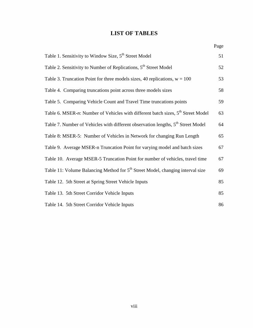
LIST OF TABLES viii
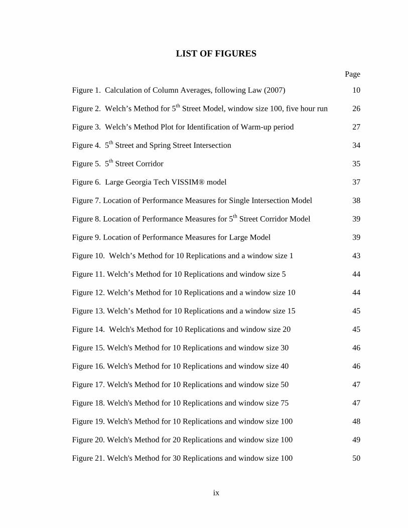
LIST OF FIGURES ix
SUMMARY xii
CHAPTER 1: INTRODUCTION 1
1.1 Need for Study 2
1.2 Study Objective 3
1.3 General Procedure 3
1.4 Study Overview 4
CHAPTER 2: LITERATURE REVIEW AND BACKGROUND 5
2.1 Defining Steady-State 5
2.2 Steady-State in Transportation 8
2.3 Methods of Truncating the Initial Transient 9
2.3.1 Graphical Methods 10
2.3.1.1 Fishman’s Method (Column Averages) 10
2.3.1.2 Welch’s Method: Moving Averages 11
2.3.2 Heuristic Methods 12
2.3.2.1 Marginal Standard Error Rule (MSER) 12
2.3.2.2 Marginal Standard Error Rule (MSER-5) 13
2.3.2.3 Conway’s Rule 13
2.3.2.4 Crossing of the Means Rule 14
2.3.2.5 Replicated Batch Means 14

v
2.3.3 Statistical Methods 15
2.3.3.1 Randomization Test 15
2.3.3.2 Welch’s Regression-Based Method 16
2.3.3.3 N-Skart 16
2.3.3.4 Automated Simulation Analysis Procedure (ASAP) 17
2.3.4 Initialization Bias Tests 18
2.3.5 Hybrid Methods 18
2.3.5.1 Statistical Process Control 18
2.4 Methods currently used by simulation models 20
2.4.1 PTV Vision – VISSIM® 21
2.4.2 McTrans – CORSIM’s Volume Balancing 21
2.4.3 Caliper Corporation – TransModeler® 22
2.5 Selection of Methods 22
CHAPTER 3: METHODOLOGY 24
3.1 Welch’s Method 24
3.1.1 Selecting Window Size 28
3.1.2 Travel Times using Welch’s Method 28
3.2 Marginal Standard Error Rule (MSER-5) 29
3.2.1 Batch Size Selection 30
3.2.2 Using MSER on Multiple Replications 30
3.3 Volume Balancing (CORSIM) 31
3.3.1 Multiple Replications 31
3.4 VISSIM® Model Characteristics 32

vi
3.4.1 VISSIM® Overview 32
3.4.2 Design of Experiment 33
3.4.3 5th Street and Spring Street Intersection 34
3.4.4 5th Street Corridor 35
3.4.5 Large Georgia Tech Network 36
3.5 Performance Measures 37
3.6 VISSIM® Limitations 40
CHAPTER 4: RESULTS 42
4.1 Welch’s Method 42
4.1.1 Selection of Window Size 42
4.1.2 Sensitivity to Number of Replications 51
4.1.3 Change in Model Size 53
4.1.4 Welch’s Method using Travel Time 54
4.1.5 Analysis of Welch’s Method 60
4.2 Marginal Standard Error Rule (MSER) 60
4.2.1 Sensitivity to Batch Size, Observation Size 62
4.2.2 Sensitivity to Observation Length 64
4.2.3 Sensitivity to Simulation Run Length 65
4.2.4 Change in Volume and Model Size 65
4.2.5 Travel Time Comparison 67
4.2.6 Analysis of MSER 68
4.3 Volume Balancing Method 68
4.3.1 Sensitivity to Interval Size 69

vii
CHAPTER 5: DISCUSSION AND CONCLUSION 73
5.1 Analysis of Welch’s Method 73
5.1.1 Issues/Criticisms of Welch’s Method 74
5.2 Analysis of MSER 76
5.2.1 Issues/Criticisms of MSER 77
5.3 Analysis of the Volume Balancing Method 79
5.4 Limitations 81
5.5 Conclusion 82
APPENDIX A: DEVELOPMENT OF VISSIM® MODEL 83
APPENDIX B: ADDITIONAL PLOTS FOR WELCH’S METHOD 87
APPENDIX C: MSER GRAPHS 89
APPENDIX D: VISUAL BASIC™ CODE 92
REFERENCES 107
viii
LIST OF TABLES
Page
Table 1. Sensitivity to Window Size, 5th Street Model 51
Table 2. Sensitivity to Number of Replications, 5th Street Model 52
Table 3. Truncation Point for three models sizes, 40 replications, w = 100 53
Table 4. Comparing truncations point across three models sizes 58
Table 5. Comparing Vehicle Count and Travel Time truncations points 59
Table 6. MSER-n: Number of Vehicles with different batch sizes, 5th Street Model 63
Table 7. Number of Vehicles with different observation lengths, 5th Street Model 64
Table 8: MSER-5: Number of Vehicles in Network for changing Run Length 65
Table 9. Average MSER-n Truncation Point for varying model and batch sizes 67
Table 10. Average MSER-5 Truncation Point for number of vehicles, travel time 67
Table 11: Volume Balancing Method for 5th Street Model, changing interval size 69
Table 12. 5th Street at Spring Street Vehicle Inputs 85
Table 13. 5th Street Corridor Vehicle Inputs 85
Table 14. 5th Street Corridor Vehicle Inputs 86
ix
LIST OF FIGURES
Page
Figure 1. Calculation of Column Averages, following Law (2007) 10
Figure 2. Welch’s Method for 5th Street Model, window size 100, five hour run 26
Figure 3. Welch’s Method Plot for Identification of Warm-up period 27
Figure 4. 5th Street and Spring Street Intersection 34
Figure 5. 5th Street Corridor 35
Figure 6. Large Georgia Tech VISSIM® model 37
Figure 7. Location of Performance Measures for Single Intersection Model 38
Figure 8. Location of Performance Measures for 5th Street Corridor Model 39
Figure 9. Location of Performance Measures for Large Model 39
Figure 10. Welch’s Method for 10 Replications and a window size 1 43
Figure 11. Welch’s Method for 10 Replications and window size 5 44
Figure 12. Welch’s Method for 10 Replications and a window size 10 44
Figure 13. Welch’s Method for 10 Replications and a window size 15 45
Figure 14. Welch's Method for 10 Replications and window size 20 45
Figure 15. Welch's Method for 10 Replications and window size 30 46
Figure 16. Welch's Method for 10 Replications and window size 40 46
Figure 17. Welch's Method for 10 Replications and window size 50 47
Figure 18. Welch's Method for 10 Replications and window size 75 47
Figure 19. Welch's Method for 10 Replications and window size 100 48
Figure 20. Welch's Method for 20 Replications and window size 100 49
Figure 21. Welch's Method for 30 Replications and window size 100 50

x
Figure 22. Welch's Method for 40 Replications and window size 100 50
Figure 23. Welch's Method using Travel Time, medium model, 10 replications, w=1 55
Figure 24. Welch's Method using Travel Time, medium model, 20 replications, w=50 56
Figure 25. Initial Warm-up of Welch's Method using Travel Time, medium model, 20
replications, w = 50 57
Figure 26. Welch's Method for Travel Time, large model, 40 replications, w = 50 58
Figure 27. Welch's Method for Travel Times, large model, 40 replications, w = 50 59
Figure 28. Sample plot of the MSER-5 statistic for an individual run 61
Figure 29. Frequency of Occurrences of truncation points for MSER-5 62
Figure 30. Cumulative Distribution Function for MSER-5 truncation values 62
Figure 31. Average MSER-n Truncation Point for varying model sizes 66
Figure 32. Percentage Difference in Vehicle Count, using 5-second intervals 70
Figure 33. Percentage Difference of Vehicle Count, using 25-second intervals 71
Figure 34. Percentage Difference of Vehicle Count, using 60-second intervals 71
Figure 35. Percentage Difference of Vehicle Count, using 100-second intervals 72
Figure 36. Confidence Interval (95%) added to Welch’s Method 75
Figure 37. Percentage Difference of Vehicle Count for Large network, (60-second
interval) 80
Figure 38. The three Model Sizes and relative location within the large model 84
Figure 39. Welch's method for small network, 40 replications, w = 100 87
Figure 40. Welch's Method for Identification of warm-up, Small network, 40
replications, w = 100 87
Figure 41. Welch's Method for large network, 50 replications, w = 150 88

xi
Figure 42. Welch's Method for Identification of warm-up, Large network, 50
replications, w = 150 88
Figure 43. Cumulative Distribution Function: MSER-5, small model, low volume 90
Figure 44. Frequency of Occurrences: MSER-5, small model size, low volume 90
Figure 45. Cumulative Distribution Function: MSER-5, large model, low volume 91
Figure 46. Frequency of Occurrences: MSER-5, small model size, low volume 91

xii
SUMMARY
All computer simulation models require some form of initialization before their
outputs can be considered meaningful. Simulation models are typically initialized in a
particular, often “empty” state and therefore must be “warmed-up” for an unknown
amount of simulation time before reaching a “quasi-steady-state” representative of the
systems’ performance. The portion of the output series that is influenced by the arbitrary
initialization is referred to as the initial transient and is a widely recognized problem in
simulation analysis. Although several methods exist for removing the initial transient,
there are no methods that perform well in all applications.
This research evaluates the effectiveness of several techniques for reducing
initialization bias from simulations using the commercial transportation simulation model
VISSIM®. The three methods ultimately selected for evaluation are Welch’s Method,
the Marginal Standard Error Rule (MSER) and the Volume Balancing Method currently
being used by the CORSIM model. Three model instances – a single intersection, a
corridor, and a large network – were created to analyze the length of the initial transient
for varying scenarios, under high and low demand scenarios.
After presenting the results of each initialization method, advantages and
criticisms of each are discussed as well as issues that arose during the implementation.
The results for estimation of the extent of the initial transient are compared across each
method and across the varying model sizes and volume levels. Based on the results of
this study, Welch’s Method is recommended based on is consistency and ease of
implementation.
1
CHAPTER 1
INTRODUCTION
Over the past several decades, computer simulation has become an increasingly
vital instrument for the analysis of transportation networks. By using simulation,
complex networks can be analyzed in a risk-free environment to test assumptions and
preview possible outcomes to determine their potential for implementation [1].
Simulation provides an enormous amount of flexibility to manipulate conditions that
could influence the operation of the network. For instance, if an impact analysis of the
closure of two lanes due to an accident or construction is desired, simulation can be used
to model the impact on the network without the need to physically close the two lanes.
Another example would be if several proposals for the configuration of an interchange
are being considered, an analyst can run a computer simulation model of each alternative
to see which proposal can maximize the operational efficiency.
The ability to integrate traffic demand forecasting into simulation models can be
extremely useful for transportation planning purposes. Simulations can be utilized to
model the performance of the existing roadway under future demands to help determine
which arterials cannot handle future capacity and need expanding. Given the myriad of
ways transportation simulation can be used to critically analyze travel conditions, it is
extremely important that the data processing aspect of the simulation analysis be
fundamentally sound. One area requiring additional development is guidelines to govern
the initialization of transportation simulation models in the determination of when it is
appropriate to begin collecting statistics.

2
The simulation start-up problem is of significant interest and has been studied
greatly in literature. When a model is initialized in a condition uncharacteristic of steady-
state, bias may be introduced into determined estimators leading to inaccurate results.
There are two common methods of mitigating the initialization bias problem. The most
common approach is truncation, or discarding the initial data influenced by the starting
conditions. The second approach is intelligent initialization, or starting the model in a
state with a high probability of equilibrium. However, it is not always convenient or
even practical to start the simulation is such a state [2]. More importantly, determining
what equilibrium means in a transportation model can be difficult and arbitrary. For
example, determining a priori how many vehicles to queue at each light, where to place
all the vehicles, and what initial speed is nearly impossible in most instances.
A possible challenge to the use of simulation models for analysis is determining if
the given model reaches steady-state. For instance, some argue that transportation
models never achieve stationarity because they not converge on a constant value [3].
Due to the nature of traffic signals, vehicles arrive in platoons and travel times can
fluctuate substantially over the course of several minutes. Thus, as a part of this effort a
definition of steady-state will also be established.
1.1 Need for Study
The need to eliminate initialization bias, also known as the start-up problem, is a
widely recognized challenge with simulation analysis. This occurs because non-
terminating simulations do not have predefined run lengths or initial conditions. The
processes must be initialized arbitrarily, which creates bias in steady-state parameter
3
estimates. Although methods of removing initialization bias exist, there is currently no
largely accepted method that performs suitably in all applications. Additionally, there is
an overall negligence of the initial transient problem in practice [4]. Robinson (2005)
stated that “the availability of commercial simulation software has placed simulation
model development into the hands of non-experts by removing the need for a detailed
knowledge of programming code” [5]. As a result, many simulation models are likely
being improperly used.
1.2 Study Objective
The purpose of this study is to analyze the effectiveness of several techniques in
eliminating initialization bias from transportation simulation models. A survey of the
various methods will be discussed, and the top three methods will be compared in detail
to examine their performance. The performance of these truncation methods will be
tested on a simulation model using PTV-VISSIM® 5.10.
1.3 General Procedure
The general framework that will be used to analyze the initialization bias
mitigation methods is outlined below:
1. Steady-state in simulation must first be defined.
2. Existing methods of removing initialization bias are surveyed.
3. Three truncation methods are selected based on popularity and effectiveness.
4. VISSIM® models are created for varying network sizes.
5. Measures of Effectiveness (MOE) for each network are determined.

4
6. Each truncation method will be applied to the selected MOE under non-
congestion conditions.
7. The methods will be reapplied for cases when the network approaches congestion.
1.4 Study Overview
This study compares the proposed initialization bias truncation methods on three
different networks. First the methodology is tested on a single intersection modeled after
the 5th Street and Spring Street intersection in Atlanta, Georgia. Second, this study area
is expanded to a corridor of 5th Street consisting of five signalized intersections. Finally,
a large network encompassing the Georgia Tech campus and surrounding area is
analyzed, including the 5th Street corridor. This large network is approximately 18 by 22
blocks and consists of 87 signalized intersections. Each network is simulated for both
under-capacity and near-capacity conditions. This analysis allows for a study of the
impact of network size and traffic demand on the initial transient in the transportation
setting.
5
CHAPTER 2
LITERATURE REVIEW AND BACKGROUND
The purpose of this research is to determine when a simulation model has reached
equilibrium, or steady-state. This will allow for the identification and elimination of the
initial transient and the determination of unbiased (regarding model start-up) performance
measures. However, before the initial transient may be identified a general definition of
steady-state must be established as well as a definition of steady-state specific to
transportation simulation models. For transportation simulation applications this effort
will focus on microscopic simulation models.
After defining the initial transient current methods of removing the initial
transient in simulation output data found by reviewing relevant literature will be
introduced. The majority of this literature was selected from the Proceedings of the
Winter Simulation Conference, the European Journal of Operational Research, and the
Naval Research Logistics Quarterly. The methods currently being used by the simulation
tools VISSIM®, CORSIM, and TransModeler are examined as well. Finally, three
methods selected for implementation within this research are identified and further
discussed.
2.1 Defining Steady-State
Simulations can be classified as either terminating or nonterminating. A
terminating simulation has a “natural” event that specifies the duration of each run [3].
An example would be a restaurant open from 8:00 A.M. to 10:00 P.M. and observing the

6
number of transactions occurring within that finite time period. A non-terminating
simulation has no natural event to specify the run length [3]. An example is a
continuous process with no ending conditions, such as traffic flowing on a freeway. In
this study the steady-state parameters of interest are estimated from non-terminating
simulations. Two strategies for calculating the steady-state mean of the performance
measure of interest are:
1. Fixed sample size – A single run of arbitrary length is conducted and a confidence
interval is constructed about the sample mean.
2. Sequential procedures – Simulation length is sequentially increased until an
“acceptable” confidence interval is achieved [6].
This study focuses on fixed sample size procedures that can be used after the simulation
has been performed for a predefined amount of time, long enough to allow the model to
reach a steady-state. Fixed sample size procedures are the primary considerations as
much of current transportation simulation practice and tools follow fixed sample size
techniques. Future research efforts will explore the use of sequential procedures to
determine if a more significant change to the current state of the practice can realize
significant analysis benefits.
Most transportation simulations (e.g. VISSIM® which is used in this effort)
incorporate stochastic distributions (for speed, acceleration, deceleration, and various
driver behavior characteristics) due to the inherently variable nature of traffic[7]. A
stochastic process is “a collection of similar random variables ordered over time,” and
can either be discrete or continuous-time stochastic processes [6]. As the simulation
models use random variables as input, the simulation output data vary randomly over a
7
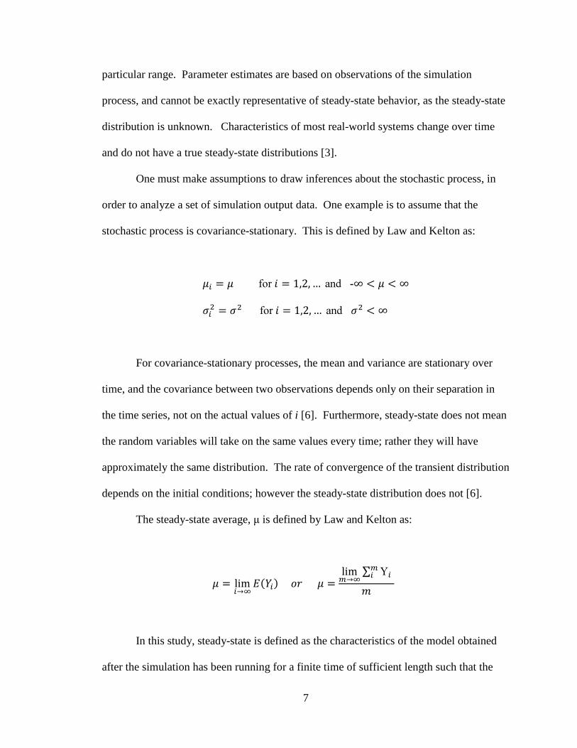
particular range. Parameter estimates are based on observations of the simulation
process, and cannot be exactly representative of steady-state behavior, as the steady-state
distribution is unknown. Characteristics of most real-world systems change over time
and do not have a true steady-state distributions [3].
One must make assumptions to draw inferences about the stochastic process, in
order to analyze a set of simulation output data. One example is to assume that the
stochastic process is covariance-stationary. This is defined by Law and Kelton as:
�� � � for � � 1,2, … and -∞ � ∞
��� � �� for � � 1,2, … and �� ∞
For covariance-stationary processes, the mean and variance are stationary over
time, and the covariance between two observations depends only on their separation in
the time series, not on the actual values of i [6]. Furthermore, steady-state does not mean
the random variables will take on the same values every time; rather they will have
approximately the same distribution. The rate of convergence of the transient distribution
depends on the initial conditions; however the steady-state distribution does not [6].
The steady-state average, µ is defined by Law and Kelton as:
� � lim���
����� �� � � lim���
∑ Y��� �
In this study, steady-state is defined as the characteristics of the model obtained
after the simulation has been running for a finite time of sufficient length such that the

8
output is “relatively free of the influence of initial conditions” [8]. This definition is
inherently subjective as the user is responsible for choosing the run length and depends
on the user’s interpretation of ‘relatively free of influence’. Determining the length of the
simulation run depends on the size of the network, however, in steady state the
characteristics of model should take on the same distributions compared to a model run
for an extremely long time (infinite in theory).
Analysts are typically interested in several performance measures from the output
data. Each separate performance measures could reach steady-state at different times,
thus it is important to check each performance measure for initialization bias and use a
start-up time that is adequate for all of them [9].
2.2 Steady-State in Transportation
Transportation simulation is similar to a queuing system, but varies because: 1) in
many instances faster vehicles can overtake slower vehicles without having to wait
behind, 2) vehicles can change lanes easily as opposed to often fixed queues in servers, 3)
capacity is a continuous constraint over the entire roadway, not just a point constraint, 4)
congestion can occur unexpectedly, and 5) traffic demands indicate strong time-series
patterns rather than random distributions [1].
There are several performance measures that can be used to determine when a
transportation simulation model is in steady-state. The measures of effectiveness selected
for this experiment are the number of vehicles in the network and the average travel times
across the network. Calculating the number of vehicles in the network for a given time
interval allows for the determination of when the entering and exiting volumes are
9
balanced, a common intuitive measure of when the system is “full”. Travel times record
the amount of time it takes a vehicle to traverse the model which is made up of the free
flow time plus the delay encountered by the vehicle. Travel time (along with delay as a
standalone component) is a common utilized performance metric. If the model does not
reach a steady-state, it is expected that the number of vehicles in the network and the
travel times would constantly increase.
It is noted that other performance metrics could be utilized to test for steady state,
e.g., queue length, average link speed, etc. However, in this effort the number of vehicles
in the network and travel time are utilized due to their ability to aid in the intuitive
understanding of model performance and their common use in practice. Future efforts
however should be undertaken to consider the potential benefits of alternative measures
or combinations of measures.
2.3 Methods of Truncating the Initial Transient
A survey of methods used to delete the data affected by the initial transient of
discrete event stochastic simulation models is discussed. These methods of initializing
simulation models seek to provide more accurate results for the steady-state estimates of
the mean. The methods can be grouped into the following categories as described by
Robinson (2007): graphical, heuristic, statistical, initialization bias testing, and hybrid
methods [10].

10
2.3.1 Graphical Methods
The most common methods to identify the initial transient are graphical
procedures. Graphical procedures consist of a visual inspection of the time series to
determine the extent of the initial transient. A major advantage is the simplicity of these
methods and their reliance on few assumptions. These methods are typically highly
subjective as the truncation points could vary based on the judgment or experience of the
analyst.
2.3.1.1 Fishman’s Method (Column Averages)
Two types of error present in discrete event simulation are sampling error (caused
by random input) and systematic error (due to the initial transient) [8]. To detect the
systematic error, multiple independent replications are needed to reduce the sampling
error. Fishman proposed to plot the sequence of column averages to visually determine a
suitable warm-up [11]. To calculate the column average, independent replications of a
predefined length are lined up in rows and the average value is determined for each
observation. In the Figure below, Yij represents the jth observation of the ith replication.
Replication 1 Y11, Y12, Y13, Y14, … , Y1 j
2 Y21, Y22, Y23, Y24, … , Y2 j . . . . .
.
. . . . .
. . . . . .
.
n Yn1, Yn2, Yn3, Yn4, … , Yn j
Column Averages
Figure 1. Calculation of Column Averages, following Law (2007)
1Y 2Y 3Y 4Y jY

11
Fishman’s method requires multiple replications in parallel and an experienced
user to determine the warm-up from the graph. The steps for Fishman’s method are as
follows:
1. Choose the run length t and number of replications n.
2. Compute the average values over every replication at each time step.
3. Plot the column, and if a the graph “fails to reveal a suitable warm-up,”
iteratively increase the run length and the number of replications [8].
2.3.1.2 Welch’s Method: Moving Averages
Welch’s method is a simple and general technique for determining when a model
reaches steady-state that can be considered an extension of Fishman’s Method [6, 11].
Welch’s Method consists of plotting a sliding window of the sequence of column
averages in an attempt to reduce the effects of the systematic error. It requires multiple
replications with the goal of determining the smallest window size that best smoothes the
plot of the moving averages, allowing the sequence to converge to a constant value where
the truncation point can be visually identified. Welch (1983) stated that the window
should be “long enough to remove short term fluctuations but not so long as to distort the
long term trend” [12].
A major concern in applying Welch’s procedure in practice is the large number of
replications required if the process is highly variable. Another disadvantage is that
smoothing the data can lead to inaccurate results. Finally, the determination of the
“smoothness” of the plot and the convergence point is based on the user’s subjective
judgment.

12
2.3.2 Heuristic Methods
These methods provide definitive rules or formulas to determine the length of the
warm-up period. The advantages of these methods are lack of user specific subjectivity,
ease of implementation, and the few assumptions needed. However, if the output series
is not visually inspected, important patterns could be overlooked.
2.3.2.1 Marginal Standard Error Rule (MSER)
First proposed by White in 1997 as the Marginal Confidence Rule, the goal of this
method is to find the truncation point that best “balances the tradeoff between improved
accuracy (elimination of bias) and decreased precision (reduction in the sample size)”
[13]. A key assumption of the MSER is the observations in the second half of the
simulation are closer in value to the true steady-state mean. White proposes to “select a
truncation point that minimizes the width of the marginal confidence interval about the
truncated sample mean” [14]. The expression for the optimal truncation point, dj is
shown below:
��� � arg min���� �
� 1�n�j� � d�j�!� " #���$� � �%�,�$�&��
����
'
MSER applies to the raw output series, Yi (j) and the truncation point, dj is
selected at the minimum value of this function. MSER tests to see if an observation prior
to the proposed truncation point is representative of the sequence observed after this
point, and if including the prior observations would increase the marginal confidence in
the estimator [13].

13
2.3.2.2 Marginal Standard Error Rule (MSER-5)
A slight modification to MSER, this method examines a series of batch averages
and uses the same formula to compute the optimal truncation point. White Jr. et al.
(2000) determined the performance of MSER can be improved by using batch means,
specifically a batch size of five [14]. The process is calculated using nonoverlapping
batches; the rule evaluates the removal of leading batches and calculates the width of the
confidence interval on the remaining data set. After the optimal truncation point has
been selected, the resulting truncated batch means are assumed to have minimal MSE and
be free of initialization bias [15].
This method has been shown to produce desirable results by minimizing the width
of the confidence interval, however, one critical problem found with the MSER-5 method
is the technique can be very sensitive to outliers, which can result in poor performance.
In a study by Sandikçi and Sabuncuoğlu using MSER-5, the output data contained 8
extreme data points and the suggested truncation point was at 4800 observations.
However, if the outliers were removed the truncation point changed to 340 observations
[4].
2.3.2.3 Conway’s Rule
Conway (1963) proposed to “truncate a series of measurements until the first of
the series is neither the maximum nor the minimum of the remaining set” [16]. This
method would not be suitable for transportation models due to the variability in the
simulation process. Output data from transportation models tends to have cyclic patterns

14
due to the operation of signal controllers, which would often result in assuming the model
has reached steady-state too early.
2.3.2.4 Crossing of the Means Rule
Proposed in by Fishman (1973), this method requires the analyst to “compute the
running cumulative mean as data are generated. Count the number of crossings of the
mean, looking backwards to the beginning. If the number of crossings reaches a pre-
specified value,” the resulting value is the proposed truncation point [17]. While the
method removes subjectivity from its application in a particular instance the method itself
remains highly subjective. It requires the user to predefine the number of crossings that
will be used, leading to arbitrary truncation points. For instance, in a study performed by
Gafarian et al. (1978), a value of three was used [18], however, little justification exists
for applying this results directly to the transportation application.
2.3.2.5 Replicated Batch Means
This method attempts to combine independent replications (IR) and batch means
(BM) to estimate steady state characteristics. Using the IR method, r independent runs
are performed and the sample average is computed for each run. Conversely, the BM
method consists of performing a single, long run and dividing the output into b
continuous batches [19]. There is a tradeoff between using a single, long run and making
many replications:
• Using IR, the replications are independent of each other; however, each trial is
influenced by initialization bias created from starting up the simulation run.

15
• With BM, initialization only occurs in the first batch, but adjacent batches are
usually correlated to each other [19].
Replicated batch means (RBM) combines the two methods in an attempt to
benefit from each of the method’s advantages. Argon et al. (2006) propose conducting a
few independent replications, each including the same number of batches[20]. Numerical
results from the 2006 study produced confidence interval estimates that were similar to
substantially better than results obtained by BM [19].
2.3.3 Statistical Methods
These methods rely on the statistics principles to determine the warm-up period.
Disadvantages tend to include the complexity of these procedures, constraining
assumptions, and increased computing time.
2.3.3.1 Randomization Test
The Randomization test sets a null hypothesis that there is no initialization bias.
The sample is divided into b batches and the grand mean of the first batch is compared to
the grand mean of the remaining batches. If the difference is significant, the null
hypothesis is rejected, the batches are regrouped, and the second batch is added to the
first group. The grand means of the first two batches are compared to the remaining b–2
batches to see if they are significantly different. This process is repeated until the
hypothesis is accepted and the transient is detected. The second group of batches
represents the steady-state simulation output [17, 21]. As with the previous methods the

16
users must still make a number of subjective assumptions, for instance, the batch size can
significantly influence results.
2.3.3.2 Welch’s Regression-Based Method
The goal of this statistical procedure is identify an appropriate truncation point
and run length by fitting a straight regression line to the second half of the data. After the
output is grouped into batches, a straight line is fit to the batch means of the second half
of the data using generalized least squares (GLS) [22]. If the slope of the line is
“significantly different from zero,” the run length must be increased. Once enough data
is collected, a reverse pass though the sequence is performed and the simulation is
consider to be in steady state as long as the fitted line continues to have a zero slope [22].
However, Law and Kelton (2000) noted several theoretical limitations of this approach,
such as the fundamental assumption that the process converges to µ monotonically, and
declined to test it further [3]. Other criticisms noted by Hoad et al. (2008) are the high
number of parameters needed (nine), the procedure is computationally intensive and can
be complex to execute [23].
2.3.3.3 N-Skart
The purpose of the N-Skart method is to create a confidence interval (CI) for the
mean with the desired coverage probability (1 – α) specified by the user. This is achieved
by employing von Neumann’s Randomness test to spaced batch means to determine the
point after which the batches are independent and uninfluenced by the initial conditions
[15]. N-Skart makes modifications to the non-spaced batch means’ CI to correct the
17
underlying skewness and autocorrelation. “The skewness adjustment is based on the
Cornish-Fisher expansion for the t-statistic, and the autocorrelation adjustment is based
on a first-order autoregressive approximation to the batch means autocorrelation
function” [15].
When compared to the MSER-5 method, N-Skart showed significantly less bias
and variance. However, N-Skart is significantly more complicated and more efficient
versions are needed to reduce processing time [15].
2.3.3.4 Automated Simulation Analysis Procedure (ASAP)
ASAP is an algorithm for simulation output analysis based on nonoverlapping
batch means. For ASAP3 (a refinement of ASAP and ASAP2), the batch size is
increased until the batch means pass the Shapiro-Wilk test for multivariate normality,
ASAP3 fits a first-order autoregressive time series model to the batch means [24]. Next,
ASAP3 delivers a correlation-adjusted confidence interval (CI). In the case study
reported in Steiger et al. (2004), the simulation is initially divided into 256 batches (with
400 long run independent replications being performed). The first 4 batches are ignored
and every other group of 4 consecutive batches are selected and tested for multivariate
normality. If failed, the batch size is increased by a factor of √2. Correlation between
adjacent batches is tested to ensure that it does not exceed 0.8. The confidence intervals
are then constructed and check to see if they meet the precision requirements [24].
This method requires a large amount of replications, and an analyst with a great
amount of expertise to perform. ASAP also requires a precision requirement and at this
time, it would not be suitable for transportation applications.

18
2.3.4 Initialization Bias Tests
The goal of initialization bias testing is to determine if bias is present in the data
due to the initial transient. The majority of these methods build upon the work of
Schruben (1982) [10]. The general procedure is to divide the output series into b batches
of equal length and subsequently group into two sets: b’ and b-b’[14]. The estimates of
the mean and variance are used to compute a test statistic which is compared to an
appropriate F distribution [14]. Hypothesis testing is performed with the null hypothesis
that no initialization bias exists. These procedures can also be used in union with
previously described methods to determine if initialization bias has been successfully
removed
2.3.5 Hybrid Methods
Hybrid methods are a combination of two methods, usually initialization bias
testing and either a graphical or heuristic method. These methods are typically complex
and can require large amounts of data [10].
2.3.5.1 Statistical Process Control
The statistical process control (SPC) method can be classified as a hybrid; a
combination of a graphical and heuristic methods. In this approach a simulation model is
considered “out of control” while in its transient phase and once it has reached steady-
state, “in-control”. The goal of the SPC method is to determine when a model is “in
control” and thus when the model is no longer influenced by its initial state [10].
The 4 steps for the SPC method are:

19
1. Perform experiment and collect data.
2. Test the second half of the data to check that it is distributed normally and not
correlated. The SPC approach must meet these two conditions, therefore:
• As simulation output is typically a correlated time series batch means
represent one method to account for this autocorrelation. However, one issue
with batch means is determining the batch size. This procedure requires that
the batch size be doubled until the null hypothesis (that there is no correlation
between batches) is accepted. The minimum batch size for which there is no
correlation is sought.
• The data must pass the test for normality at each selected batch size. Different
methods of testing for normality include:
o Chi-square test
o Kolmogorov-Smirnov test
o Anderson-Darling test
• If the number of batches is less than 20, a longer simulation run is needed.
3. Construct a control chart.
• It is assumed the process is stable during the second half of the data. Estimates
for the population mean and standard deviation are taken from this portion of
the time series.
• Three sets of control limits are calculated accordingly:
CL � �̂ , z�./√n for z = 1, 2, 3
4. Determine the initial transient.

20
• To plot the control chart, the mean, three sets of control limits, and the time-
series output are graphed.
• Rules for determining when the series is “in control” and “out of control” are
given that are based on where the data falls within the three sets of control
limits [10].
Montgomery and Runger (1994) established the following rules to determine
when the process is “out of control”:
• A point plots outside a 3-sigma control limit.
• Two out of three consecutive points plot outside a 2-sigma control limit.
• Four out of five consecutive points plot outside a 1-sigma control limit.
• Eight consecutive points plot on one side of the mean [10].
Bias, coverage, and the expected half-length of the confidence interval are the
performance measures are evaluated by Robinson. Using the SPC method easily
increased the accuracy of the steady-state parameters compared to not deleting any initial
data [10]. However, it is important to note that this method (as well several others
discussed) assumes the model is in steady-state for the second half of the simulation run.
If the model fails to reach a steady state this method will likely not identify this
condition, potentially erroneously identifying the end of the initial transient.
2.4 Methods currently used by simulation models
A survey of three traffic simulation models was conducted. Technical support
for two of these models was contacted to see how they approached the warm-up problem
in their respective software, and if the simulation models had built-in methods of
21
initializing the network. Two of the three models have a built in function to determine
when the network has reached “equilibrium”.
2.4.1 PTV Vision – VISSIM®
Correspondence was made with support at PTV-VISSIM® June 7, 2010 to
inquire how they mitigate the initialization bias problem. The response was the length of
the warm-up period is always dependent on the size and characteristics of the network,
and that this seeding period should be at least as long as the travel time of the longest
possible path through the network. Further correspondence was made (August 2, 2010)
to ask if PTV was planning on implementing a built-in method of determining
equilibrium in future releases, similar to some of its competitors. To their knowledge, no
such procedure is in progress.
2.4.2 McTrans – CORSIM’s Volume Balancing
No contact was made with CORSIM, however their built-in equilibrium
procedures were studied. The Federal Highway Administration created a set of
guidelines for applying simulation analysis entitled “Traffic Analysis Toolbox” with
Volume IV containing Guidelines for Applying CORSIM [25]. Before it is acceptable to
start accumulating statistics, CORSIM first determines when the model has reached
equilibrium. To do this, there is a built-in heuristic method that compares the number of
vehicles in the network at consecutive time intervals. It determines equilibrium has been
reached “if the difference between the current interval and the previous interval is less
than eight percent and the difference between the previous interval and the one before it

22
was less than 12 percent… If those conditions have not been met, but the difference
between the current interval and the previous interval is less than six percent” the model
has reached equilibrium [25]. The user has the option to enter a maximum initialization
time and once it has been reached, the model can either collect data if it is in equilibrium,
or abort if it is not. It can be helpful to force the maximum initialization time if the
model appears to incorrectly determine it is in equilibrium.
There are some disadvantages of using this method to determine equilibrium.
First, if a small time interval is chosen (such as one second), this method could determine
equilibrium has began prematurely because the volumes would not be expect to change
significantly in such a short period. Similarly, a large model with high volumes could
terminate the initialization period too soon because the percentage change in volume
would become less sensitive [25].
2.4.3 Caliper Corporation – TransModeler®
Contact was made with a transportation engineer at Caliper Corporation August
10, 2010 in inquire about the equilibrium capabilities of TransModeler®. The response
was that TransModeler® does implement a method of comparing the number of vehicles
in the network similar to CORSIM, however it is optional. Caliper continually surveys
research literature for other possible methods.
2.5 Selection of Methods
Hoad et al. (2008) performed a seminal study on the existing methods of
estimating the length of the warm-up period in hopes of producing an automated

23
procedure to be included in simulation software [23]. The authors conducted a
comprehensive review of literature and found 42 methods for detecting the extent of the
warm-up. These methods were evaluated and graded based on the following criteria:
accuracy and robustness of method, simplicity of the model, ease of potential automation,
generality, number of parameters required, and computing time [23]. The list was
narrowed down to six methods for further evaluation, excluding graphical methods due to
their need for human intervention. Of the six methods, MSER-5 substantially
outperformed the rest while the other methods either severely underestimated the
truncation point or required an extremely large number of replications.
The criteria that were used to determine the selected methods for this study are
their ability to be implemented, their effectiveness, and their popularity. While the
graphical methods were not included in the study performed by Hoad et al. (2008)
because of the difficulty automating the procedure [23] this experiment will evaluate the
graphical procedure, Welch’s Method, based on its simplicity and overwhelming
popularity. MSER-5 will also be implemented in this study due to its effectiveness,
frequent use in the industry, and ease of implementation. A third method that will be
examined is the volume balancing method currently used by CORSIM and
TransModeler®.

24
CHAPTER 3
METHODOLOGY
The truncation methods discussed earlier were separated into the following
categories: graphical, heuristic, statistical and initialization bias testing. Of the graphical
procedures proposed, Welch’s Method is widely used and perhaps the most referenced
method in literature. The steps needed to implement this procedure are detailed in this
chapter. For the heuristic approaches, it appears MSER-5 is the most effective method
and would be most applicable for this experiment. The formula for the MSER heuristic is
listed in this chapter, as well as issues with implementation. The third method selected is
the volume balancing procedure used by CORSIM (and similarly by TransModeler®),
which a simple mathematical heuristic. This is selected as it is the only method identified
as commonly used in transportation microscopic simulation applications. Each
methodology will first be performed on the number of vehicles in the network to
determine steady-state. Next, the network travel times will be examined and each
method reapplied.
3.1 Welch’s Method
The steps and equations for calculating Welch’s Method of moving averages for a
window size, w are listed below [3, 6]:
1. A number of replications n ≥ 5 is performed, each of length m, where m is much
larger than anticipated truncation point. The observations are averaged over all
replications at each time-step to create the average process, �.1

25
3. The moving averages, �%�2� are plotted for several values of widow size, w. An
initial value for w is 1, and then increased in increments of 1, where w ≤ m/4.
�%��2� �3445446
122 7 1 " �%����
����
if � � 2 7 1, … , � � 212� � 1 " �%������
��������
if � � 1, … , 2 944:44;
As shown above, a window size w consists of the average of (2w + 1)
observations. The smallest value of w for which the plots are “reasonable
smooth” is selected.
4. If no value of w is satisfactory, the number of replications is increased.
5. The truncation point is selected visually from the moving averages plot [3, 6].
Welch proposes starting with n = 5 or 10 replications, based on computing cost
and time. For this experiment, we started with 10 replications and increased the number
of replications if a sufficient window size could not be chosen. Based on the expected
truncation value, a simulation length of five hours was selected. This run length should
be more than sufficient for all transportation models tested to reach steady state well
before the halfway point in the model. To implement Welch’s Method an Excel™
spreadsheet was created to generate plots of incrementally increasing window sizes. The
data output was averaged over a defined number of replications (initially 10) using a
separate script. In this instance the data output is a snapshot of the number of vehicles in
26
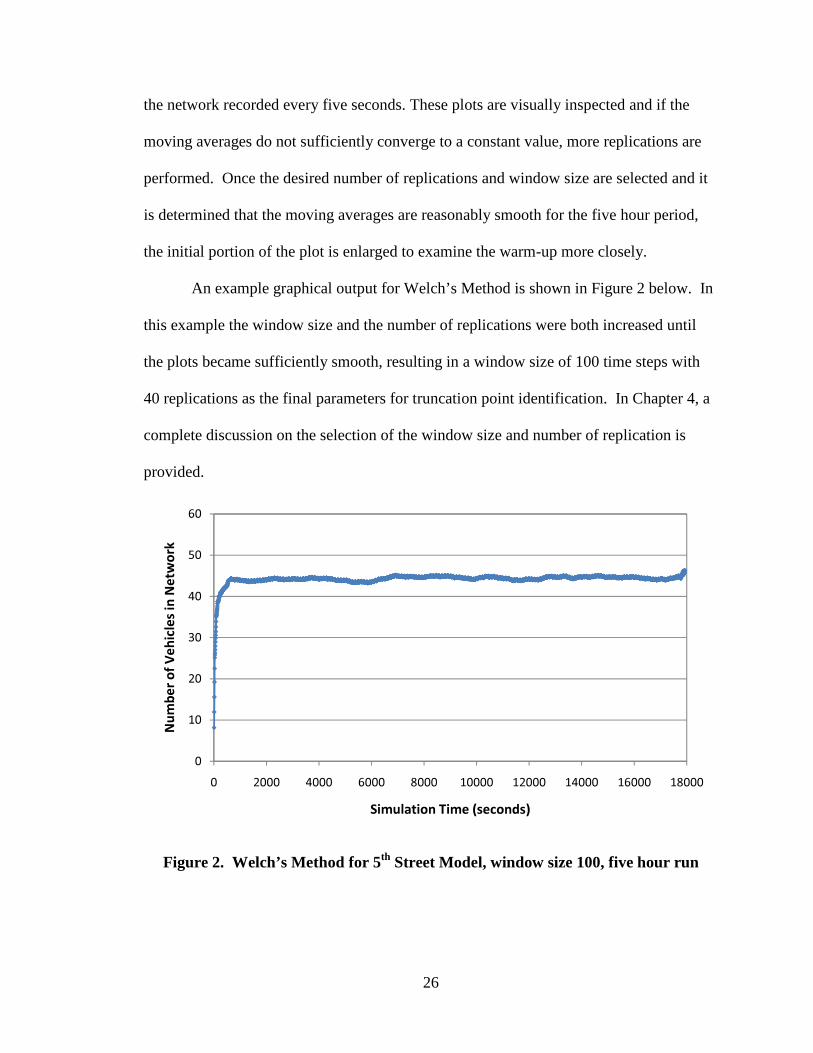
the network recorded every five seconds. These plots are visually inspected and if the
moving averages do not sufficiently converge to a constant value, more replications are
performed. Once the desired number of replications and window size are selected and it
is determined that the moving averages are reasonably smooth for the five hour period,
the initial portion of the plot is enlarged to examine the warm-up more closely.
An example graphical output for Welch’s Method is shown in Figure 2 below. In
this example the window size and the number of replications were both increased until
the plots became sufficiently smooth, resulting in a window size of 100 time steps with
40 replications as the final parameters for truncation point identification. In Chapter 4, a
complete discussion on the selection of the window size and number of replication is
provided.
Figure 2. Welch’s Method for 5th Street Model, window size 100, five hour run
0
10
20
30
40
50
60
0 2000 4000 6000 8000 10000 12000 14000 16000 18000
Nu
mb
er
of
Ve
hic
les
in N
etw
ork
Simulation Time (seconds)

27
As previously stated, to determine the point where the model reaches steady-state,
the initial portion of the above moving averages plot is enlarged. A small time period is
chosen that exceeds the anticipated truncation point and allows the analyst to visually
detect the point at which the plot becomes smooth. A visual aid is also added to the plot
to help identify when the sequence reaches the point where the plot becomes smooth. A
horizontal line is added that is equal to the average of Welch’s values in the second half
of the time series. This removes some of the subjectivity of visually detecting when the
plots reach steady-state. Figure 3 below shows the inspection of the warm-up, plotted for
the first 1200 seconds of the data shown in Figure 2 . In this example, the truncation
point was determined to be 600 seconds.
Figure 3. Welch’s Method Plot for Identification of Warm-up period
0
10
20
30
40
50
60
0 100 200 300 400 500 600 700 800 900 1000 1100 1200
Nu
mb
er
of
Ve
hic
les
in N
etw
ork
Simulation Time (seconds)

28
3.1.1 Selecting Window Size
Law and Kelton noted that “choosing w is like choosing the interval width ∆b for
a histogram” [6]. If w is too small the plots will appear ragged, and choosing a window
size too large could over-aggregate the data. Sturges’s rule is proposed to choose the
interval width ∆b for a histogram as follows:
< � =1 7 >�?� @A � =1 7 3.322 >�?�� @A
Using this formula for our case of 3600 observations would result in value of 12.8 for the
interval width. However, Law and Kelton do not believe such rules are useful and
recommend trying several different values and choosing the smallest value that best
smoothes the plot [6]. In this study, it was seen that the window size needed to be
sufficiently large to smooth out the cyclic trends due to the signalized intersections
timing plans.
3.1.2 Travel Times using Welch’s Method
As stated previously, in addition to performing Welch’s Method on the number of
vehicles in the network, Welch’s Method is applied to network travel times. While the
same method is being applied to these output values, there are some small differences in
the method application to the data. As noted the number of vehicles in the network is a
snapshot every five seconds during the simulation. However, travel time is measured
along a pre-specified path through the network. Vehicles complete their traversal of this
path randomly, based on their arrival into the network and in-network experience. Thus,
29
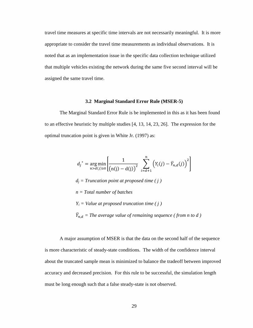
travel time measures at specific time intervals are not necessarily meaningful. It is more
appropriate to consider the travel time measurements as individual observations. It is
noted that as an implementation issue in the specific data collection technique utilized
that multiple vehicles existing the network during the same five second interval will be
assigned the same travel time.
3.2 Marginal Standard Error Rule (MSER-5)
The Marginal Standard Error Rule is be implemented in this as it has been found
to an effective heuristic by multiple studies [4, 13, 14, 23, 26]. The expression for the
optimal truncation point is given in White Jr. (1997) as:
��� � arg min���� �
� 1�n�j� � d�j�!� " #���$� � �%�,�$�&��
����
' dj = Truncation point at proposed time ( j )
n = Total number of batches
Yi = Value at proposed truncation time ( j )
�%�, = The average value of remaining sequence ( from n to d )
A major assumption of MSER is that the data on the second half of the sequence
is more characteristic of steady-state conditions. The width of the confidence interval
about the truncated sample mean is minimized to balance the tradeoff between improved
accuracy and decreased precision. For this rule to be successful, the simulation length
must be long enough such that a false steady-state is not observed.

30
3.2.1 Batch Size Selection
The first step to analyzing the MSER is to batch the data. The purpose being that
batching the observations “ensure the monotonic behavior of the decrease in confidence
interval width” [26]. It is important to recall that in the current application performance
statistics were collected every five seconds. Each snapshot at the end of five seconds is
considered a single observation. Using this original data in the application of the MSER
method will be referred to as MSER-1 because no batching is undertaken. Next, the
MSER is performed for n = 5 batches, which covers 25 simulation seconds (i.e. five, 5-
second batches). Additional results for the MSER-n will analyzed for batch sizes of 12
and 22, corresponding to 60 and 110 simulation seconds. MSER-22 was selected to
allow for a test of the method using a batch size equal to the cycle length of the major
network intersections. MSER-12 was selected to allow for a testing of the method for an
equivalent simulation time period (i.e. 60 second) as utilized by default in the CORSIM
Volume Balancing procedure.
3.2.2 Using MSER on Multiple Replications
As with Welch’s Method multiple replications helps to ensure accuracy in the
identification of the end of the initialization transient. However, the approach for using
multiple replications is different for the MSER. White Jr. (1997) noted that the Marginal
Confidence Rule (later named MSER) was not intended to be used over the average of
many replications. White stated “this rule applies to individuated output sequences and
has the inherent advantage of specifying the best truncation point for each such sequence,
rather than a single truncation point, which is best only on average across a very large

31
number of replications” [13]. Therefore, in this effort MSER is performed on each
individual replication, with 100 replications being performed. The statistics that will be
collected for the MSER truncation points are the maximum, average, and 95th percentile.
These results are shown in Chapter 4.
3.3 Volume Balancing (CORSIM)
This method could be considered a heuristic approach. In the method the percent
difference in vehicles in the network between consecutive intervals is analyzed. In
CORSIM if two consecutive percent differences are 12% or less followed by 8% or less
the model is considered to be in steady state. The calculations for this method are
straightforward; however the analyst is free to choose the interval size. The data for this
experiment was collected in five second increments to allow for flexible post processing.
This procedure will be performed on varying interval sizes as mentioned before,
including a multiple of the cycle length. CORSIM uses an interval of 60 seconds to
determine equilibrium. It is noted that no literature was found regarding the background
or development of this method.
3.3.1 Multiple Replications
Similar to the MSER, averaging multiple replications would only smooth the
initial transient truncation point to an average value, whereas we are interested in the
maximum amount of time needed to initialize individual runs of the model. Thus, this
procedure will be performed on each individual replication and the maximum, average,
and 95th percentile truncation point will be collected.

32
3.4 VISSIM® Model Characteristics
First, the characteristics of the VISSIM® simulation model are discussed. The
locations of the selected models are shown in detail and the performance measures used
to evaluate the model are discussed. The experiment design is explained to clarify which
models and conditions will be tested on Welch’s Method, MSER, and the Volume
Balancing procedure.
3.4.1 VISSIM® Overview
VISSIM® is a microscopic, behavior based traffic simulation model which uses
continuous time-step advancements to move through simulation time [7]. Networks are
created using links and connectors, where links represent sections of the road and
connections allow the vehicles to move between these links. Signal controllers, stop
signs, reduced speed areas, priority rules and most importantly, the car following model
and lane changing logic control the movement of vehicles. The accuracy of the model
depends highly on the quality of the vehicle modeling and the ability of the user to model
the respect network (e.g. intersection, arterial, freeway, etc.) geometry. VISSIM® uses a
complex psycho-physical driver behavior model developed by Wiedemann (1974) [7].
This model is based on individual drivers’ perception thresholds of slower moving
vehicles.
As VISSIM® creates a vehicle to be input into the network, specific driver
behavior characteristics are assigned randomly to each vehicle. Each driver in turn,
reacts based on the technical capabilities of his vehicle. Characteristics of each driver-
vehicle-unit can be classified into the following categories:

33
1. Technical specifications of the vehicle: (length, maximum speed, potential
acceleration, actual position in the network, actual speed and acceleration).
2. Behavior of driver-vehicle-unit: (sensitivity thresholds and ability to estimate,
aggressiveness, memory of driver, acceleration based on current speed and
driver’s desired speed).
3. Interdependence of driver-vehicle-units: (reference to leading and following
vehicles on own and adjacent travel lanes, reference to current link and next
intersection, reference to next traffic signal) [7].
3.4.2 Design of Experiment
This experiment compares the performance of initialization bias truncation
procedures in transportation microscopic simulations, utilizing VISSIM® simulation
models as the example applications. Three model sizes were developed for this study,
covering an increasing geographic area. A single signalized intersection was first
analyzed to determine the results for a small model. Next, a corridor consisting of the
single intersection and four additional signalized intersections is tested. The corridor
model is referred to as the medium network size in this study. Lastly, a large network
containing the previously analyzed corridor is studied to determine the extent of the
initial transient for varying model sizes. This would ensure that the geometry and signal
timing of the small and medium segments are consistent across the experiment.
For each model the initial experiments set the input volume at a medium demand
level, that is, non-congested traffic although reasonable demand. The actual volumes
were set based on conducting several iterations of the model and the researchers’

34
judgment of reasonable, uncongested flow. These scenarios allow for an analysis to test
the initialization bias truncation procedures with the confounding influence of
congestion. Next, the models’ input volumes are increased to the represent the peak
volume of the model operating just below capacity. Finally, each model will be loaded
over capacity to determine how each method handles the case where equilibrium is not
achieved.
3.4.3 5th Street and Spring Street Intersection
The area for this study is in Atlanta in close proximity to the Georgia Institute of
Technology (Georgia Tech) campus. The single intersection to be studied is at 5th Street
and Spring Street. Spring Street is a one-way major urban arterial with four lanes, while
5th Street is an urban local street with two lanes (one lane each direction). Figure 4 on the
following page displays the VISSIM® representation of the intersection.
Figure 4. 5th Street and Spring Street Intersection
(Figure Credit: VISSIM® with Google Earth [27] overlay)
N

35
3.4.4 5th Street Corridor
The 5th Street corridor (also known as Ferst Drive adjacent to the Georgia Tech
campus) spans from Atlantic Drive on the west, to West Peachtree Street to the east. The
model consists of a mix of four-lane major arterials with high volumes (including the
one-way pair of Spring Street and West Peachtree Street) and various two-lane local
roads with a relatively small amount of traffic primarily moving to and from the Georgia
Tech campus. Four travel time segments for this network were defined for this network,
two eastbound and two westbound. Figure 5 on the following page shows the 5th Street
corridor in VISSIM®.
Figure 5. 5th Street Corridor
(Figure Credit: VISSIM® with Google Earth [27] overlay)
N

36
3.4.5 Large Georgia Tech Network
The VISSIM® model of the Georgia Tech campus and surrounding area in
Atlanta, Georgia was developed by a graduate research student at Georgia Tech, Kate
D’Ambrosio. The network is bounded in each direction by the following streets:
• South: North Avenue
• North: 17th Street
• East: Peachtree Street
• West: Marietta Street/ Howell Mill Road
Existing geometry was extracted by overlaying a series of scaled aerial
photographs to determine the number of lanes at each intersection and the spacing
between them. The signal timings for the 5th Street corridor were obtained from the City
of Atlanta to match the existing conditions. More detailed information on the
development of the VISSIM® model is included in the Appendix. Figure 6 shows the
VISSIM® model of the large Georgia Tech network.

37
Figure 6. Large Georgia Tech VISSIM® model
(Figure Credit: VISSIM® with Google Earth [27] overlay)
3.5 Performance Measures
The performance measures chosen for this case study are number of vehicles in
the network and the network travel time. The number of vehicles in the network is
recorded every five seconds and is calculated as the instantaneous value at the end of
each five second interval. Travel time segments have been set up to record the time it
takes vehicles to pass entirely through the system for specified routes. For these routes,
probe vehicles have been inserted in the model to ensure a sufficient number of vehicles
complete the travel time segment and use the desired path. Figure 7 and Figure 8 below
N

38
show the location of the vehicle inputs and travel time segments for the single
intersection and corridor model. Figure 9 shows the location of the travel time segment
for the large Georgia Tech model.
Figure 7. Location of Performance Measures for Single Intersection Model

39
Figure 8. Location of Performance Measures for 5th Street Corridor Model
Figure 9. Location of Performance Measures for Large Model
40
3.6 VISSIM® Limitations
One major limitation of this research is the given simulation model does not
include pedestrians. Pedestrians can have a significant impact on the operation of
signalized intersections, especially near a college campus. Additionally, bicycles were
not introduced into the model. The capabilities of VISSIM® to integrate pedestrians and
bicycles were not explored, but should be considered in future research.
Another issue is the accuracy of the VISSIM® model with respect to routing
decisions, signal timing, and traffic volumes. The calibration process is an important
aspect of simulation analysis to ensure the integrity of the results. For this effort the
models were reviewed only for reasonable operations (that is, vehicle behavior and
performance that was reasonable for the given network size), not necessarily calibrated to
match field conditions for the given locations. These models have generic traffic
demands and signal timings, although where possible known field timings were utilized.
Thus, the simulations are not applicable to an operational analysis of actual conditions in
the modeled areas. However, the intent of this effort is a study of initial transient, which
may be accomplished using the given models.
One concern encountered in VISSIM® is whether or not vehicles queued off
network or vehicles disappearing were counted in the number of vehicles in the network.
Several tests were performed to determine how VISSIM® counts the number of vehicles
in the network. A simple model was created where the demand greatly exceeded the
capacity and it was found that the vehicle count only includes the vehicles that have
entered the network, and not those queued off the network. Additional tests were

41
performed to see if vehicles being removed from the model are included in the vehicles in
the network count; which they were not.
There are two main reasons vehicles would be removed from the network in our
study. The first reason is VISSIM® by default removes stalled vehicles that are unable to
make a lane change after 60 seconds to avoid unrealistic backups [7]. The second reason
is that once a vehicle has been specified a certain path on a routing decision, if that
vehicle is unable to change to a lane where it can make that turn, it will continue on
through the intersection searching for its specified path. Once it reaches the end of the
link without finding that path it is removed from the network. While this would present
an issue in measuring performance characteristics of the model, the occurrences of this
issue was minimal and is comparable to vehicles exiting the network into a parking lot.

42
CHAPTER 4
RESULTS
The results for Welch’s Method, MSER, and the Volume Balancing Method are
presented in this chapter. The sensitivity of each method’s parameters are tested and
discussed. The estimated truncation point will be given for the small, medium, and large
models, as well as a change from low volume to high volume.
4.1 Welch’s Method
For Welch’s Method, the procedures for selecting the window size and number of
replications are first discussed. Next, the sensitivity to choosing different window sizes
and number of replications is analyzed.
4.1.1 Selection of Window Size
To perform Welch’s Method, the window size w = 1 is initially evaluated and
incrementally increased until the plots become smooth. Increasing the window size will
smooth the plots of the moving averages only to a certain point; if the plots do not
sufficiently converge more replications are needed. The figures on the following pages
show the progression of increasing the window size and the number of replications until a
plot with reasonable smoothness can be selected.
The numerical value of w represents the half-width of the “window” that is used
to average the output. A window size of 10 corresponds to the average of 21
observations centered on that point in the time series. Thus, each graphed point in

43
Welch’s Method is the calculated average of 2w + 1 observations. As stated previously
an observation in this experiment represents a data point collected each 5 seconds of
simulation time. Figure 10 begins with 10 replications and a window size of 1. The
window size is increased sequentially before it no longer becomes beneficial to increase
the window size. It is important to select the smallest possible window size that produces
a reasonably smooth graph as a window size unnecessarily large will yield excessively
large initial transient truncation points.
The following plots are from the medium size model (5th Street Corridor) for low
volumes
Figure 10. Welch’s Method for 10 Replications and a window size 1
0
10
20
30
40
50
60
0 2000 4000 6000 8000 10000 12000 14000 16000 18000
Nu
mb
er
of
Ve
hic
les
in N
etw
ork
Simulation Time (seconds)

44
Figure 11. Welch’s Method for 10 Replications and window size 5
Figure 12. Welch’s Method for 10 Replications and a window size 10
0
10
20
30
40
50
60
0 2000 4000 6000 8000 10000 12000 14000 16000 18000
Nu
mb
er
of
Ve
hic
les
in N
etw
ork
Simulation Time (seconds)
0
10
20
30
40
50
60
0 2000 4000 6000 8000 10000 12000 14000 16000 18000
Nu
mb
er
of
Ve
hic
les
in N
etw
ork
Simulation Time (seconds)

45
Figure 13. Welch’s Method for 10 Replications and a window size 15
Figure 14. Welch's Method for 10 Replications and window size 20
0
10
20
30
40
50
60
0 2000 4000 6000 8000 10000 12000 14000 16000 18000
Nu
mb
er
of
Ve
hic
les
in N
etw
ork
Simulation Time (seconds)
0
10
20
30
40
50
60
0 2000 4000 6000 8000 10000 12000 14000 16000 18000
Nu
mb
er
of
Ve
hic
les
in N
etw
ork
Simulation Time (seconds)
46
Figure 15. Welch's Method for 10 Replications and window size 30
Figure 16. Welch's Method for 10 Replications and window size 40
0
10
20
30
40
50
60
0 2000 4000 6000 8000 10000 12000 14000 16000 18000
Nu
mb
er
of
Ve
hic
les
in N
etw
ork
Simulation Time (seconds)
0
10
20
30
40
50
60
0 2000 4000 6000 8000 10000 12000 14000 16000 18000
Nu
mb
er
of
Ve
hic
les
in N
etw
ork
Simulation Time (seconds)
47
Figure 17. Welch's Method for 10 Replications and window size 50
Figure 18. Welch's Method for 10 Replications and window size 75
0
10
20
30
40
50
60
0 2000 4000 6000 8000 10000 12000 14000 16000 18000
Nu
mb
er
of
Ve
hic
les
in N
etw
ork
Simulation Time (seconds)
0
10
20
30
40
50
60
0 2000 4000 6000 8000 10000 12000 14000 16000 18000
Nu
mb
er
of
Ve
hic
les
in N
etw
ork
Simulation Time (seconds)

48
Figure 19. Welch's Method for 10 Replications and window size 100
Beyond a window size of 100, the advantages of selecting a larger window size
are no longer beneficial. Thus, the plots do not appear to converge to a smooth line with
the selected number of replications. Figures 19–22 demonstrate the selection of the
number of replications needed to smooth the moving averages. Similarly to the selection
of the window size, after a certain amount of replication there is no longer significant
improvement in the smoothness of the plots. After 10 replications were examined, the
number of replications was increased by 10 each time.
In this example, 40 replications were found sufficient to result in convergence of
the moving averages. After 40 replications were selected, the process of determining the
window size was repeated and w = 100 was selected again. The next step for Welch’s
Method is to plot the initial portion of the moving averages series and visually determine
0
10
20
30
40
50
60
0 2000 4000 6000 8000 10000 12000 14000 16000 18000
Nu
mb
er
of
Ve
hic
les
in N
etw
ork
Simulation Time (seconds)

49
when the plot is “reasonably smooth”. By including the horizontal line representing the
average value over the second half of the data, the truncation point could be selected
easily.
Figure 20. Welch's Method for 20 Replications and window size 100
0
10
20
30
40
50
60
0 2000 4000 6000 8000 10000 12000 14000 16000 18000
Nu
mb
er
of
Ve
hic
les
in N
etw
ork
Simulation Time (seconds)
50
Figure 21. Welch's Method for 30 Replications and window size 100
Figure 22. Welch's Method for 40 Replications and window size 100
0
10
20
30
40
50
60
0 2000 4000 6000 8000 10000 12000 14000 16000 18000
Nu
mb
er
of
Ve
hic
les
in N
etw
ork
Simulation Time (seconds)
0
10
20
30
40
50
60
0 2000 4000 6000 8000 10000 12000 14000 16000 18000
Nu
mb
er
of
Ve
hic
les
in N
etw
ork
Simulation Time (seconds)
51
Clearly selecting the appropriate window size is a judgment call and can vary
from user to user. Each user selects the smallest possible window that can smooth (in
that users’ judgment) the data. For instance, in this example a window size of 100 was
selected by the author. To analyze the impact of user judgment, results were obtained for
two window sizes below 100 and two above 100. Table 1 below shows the truncation
points found at these different window sizes. An important trend was discovered: as the
window size increases, so does the estimated truncation point. Thus, the selection of the
window size has a significant impact on the location of the anticipated truncation point.
It is expected that some users will tend to determine more conservative truncations points
while other tend to determine short start-up periods.
Table 1. Sensitivity to Window Size, 5th Street Model
Number of Replications
Window Size
Truncation Point Low
Volume High
Volume 40 60 400 400 40 80 500 450 40 100 600 550 40 120 700 650 40 140 800 750
4.1.2 Sensitivity to Number of Replications
Law and Kelton proposed starting with five or ten replications, based on model
execution and cost [6]. In our study, ten replications were used as a starting point and the
number of replications were increased until the desired smoothness is achieved. A total
of 100 replications were performed, each with a different random seed. Ten replications

52
were randomly selected from the sample set and the average value was computed at each
time step. This sampling method was repeated to obtain the averages of 20, 30, 40, and
50 replications. The entire set was used to find the average over 100 replications. The
impact of using different numbers of replications for the medium model size is shown in
Table 2 below.
Table 2. Sensitivity to Number of Replications, 5th Street Model
Number of Replications
Window Size
Truncation Point Low
Volume High
Volume 10 100 550 550 20 100 550 550 30 100 600 550 40 100 600 550 50 100 550 550 100 100 600 550
As the number of replications is increased, it becomes easier to determine the
truncation point as the moving average plots becomes smoother. However, the same
truncation time can be read from the graph of 10 replications as that of 100 replications,
shown in Table 2 for the high volume case. The trend was evident for both the small and
large model sizes (results included in Appendix). This indicates that Welch’s Method
can provide similar results as the number of replication is increased for this model
scenario. However, it should be noted that 10 replications was used as the minimum for
this experiment; it is not believed that using one, or even five replications would produce
the same result as those from 100 replications.

53
The major factor affecting the sensitivity of the truncation point found by Welch’s
Method to the number of replications used is the variability of the output data. For highly
variable data, a large amount of replications may be needed to produce similar results.
More analysis is needed before this conclusion can be generalized, but the fact that the
results obtained from 10 and 100 replications are similar is an important finding.
4.1.3 Change in Model Size
Welch’s Method was applied to the three different model sizes: a single
intersection, a small corridor, and a large grid network. The results for the Welch’s
Method for each case are shown in Table 3 below. The truncation point was found using
replicated averages of the number of vehicles in the network for both the low and high
volume case.
Table 3. Truncation Point for three models sizes, 40 replications, w = 100
Volume Truncation Point (seconds)
Small Medium Large Low 600 650 1800 High 550 550 1700
The small and medium network sizes have very similar warm-up lengths, while
the warm-up period for the large network is almost three times as large. One reason the
small and medium network have similar warm-up times is these two models are generally
dominated by the same intersection, Spring Street and 5th Street. The small network
consists of solely this intersection while the medium model contains an additional
intersection to the east (West Peachtree Street) and three signalized intersections to the

54
west. Both Spring Street and West Peachtree Street contain five times as much volume
as that on 5th Street. Thus, the time it takes to initialize the 5th Street corridor model
depends primarily on the time it takes to warm-up the intersection at Spring Street. The
number of vehicles in the network is the performance measure evaluated, and the
intersections with higher volumes dominate the calculations. For future research, it
would be beneficial to construct an experiment where the volume difference between the
two cross streets is less drastic.
As expected the large model contains a longer initial transient period than the
smaller models. During its steady-state conditions, the large model contains fewer than
900 vehicles in the network, while the medium and small models contain an average of
84 and 41 vehicles (respectively) for the high volume case. The main factors that
determine the length of the initial transient are the distance and time a vehicle needs to
travel through the network. A model with a large number of signalized intersections
would be expected to reach steady-state at a later time because of delay encountered at
each intersection. Similarly, if the effective green time is reduced for major movements
in a network, the initial transient period would be expected to increase.
4.1.4 Welch’s Method using Travel Time
Network travel time was tested for Welch’s Method to determine if travel time is
a good indicator of the performance of corridor or network. For each model size, a route
was selected that is considered representative of the network and constitutes a large
amount of traffic. The input volume and routing decisions were modified before the
experiment was performed such that a minimum of 60 vehicles would complete the travel

55
time segment per hour. This number was selected based on the desire to have a sufficient
amount of data to perform each method by creating an observation interval of 60 seconds.
For the first iteration of Welch’s Method, 10 replications were randomly selected
and averaged. The window size was initially set at w = 1 for the medium network as
shown in Figure 23 below.
Figure 23. Welch's Method using Travel Time, medium model, 10 replications, w=1
Next, the window size is sequentially increased until the plots become
“reasonably smooth”, which could not be achieved without further replications. Using 20
replications, the window size was increased to w = 50 to produce the desired smoothness.
The moving average plots from 20 replications are displayed in Figure 24 on the
following page.
100
110
120
130
140
150
160
170
0 2000 4000 6000 8000 10000 12000 14000 16000 18000
Tra
ve
l T
ime
Me
asu
red
(se
con
ds)
Simulation Time (seconds)

56
Figure 24. Welch's Method using Travel Time, medium model, 20 replications,
w=50
The next step of analyzing Welch’s Method is to examine the initial portion of the
graph and visually select the truncation point. The first 3600 seconds of the simulation
are shown in Figure 25 on the next page. From this figure, there are two different
truncation points that can be selected. The first time the moving averages intersects the
mean (calculated over the second half of data) is at 600 seconds and then again at 1100
seconds for the second time.
100
110
120
130
140
150
160
170
0 2000 4000 6000 8000 10000 12000 14000 16000 18000
Tra
ve
l T
ime
Me
asu
red
(se
con
ds)
Simulation Time (seconds)

57
Figure 25. Initial Warm-up of Welch's Method using Travel Time, medium model,
20 replications, w = 50
An argument could be made for choosing either of these points. At 600 seconds,
the model could have reached equilibrium and is experiencing a realistic spike in
demand. Or, the analyst could interpret this graph as first reaching steady-state at 1100
seconds and the high values of travel time is not representative of the model. While both
interpretations are valid, the author selected a truncation point of 600 seconds for this
case because it is not good practice to discard data that could be representative of a
realistic steady-state condition solely based on the fact that it would have a negative
impact on the model performance statistics.
For the medium model size shown above, the plots generated from travel time
measurements are not as smooth as those generated by using the network vehicle count.
An explanation is that travel time can be a sparse measurement for small networks. For
the large model, however, this is not the case. Welch’s Method for the large network is
100
110
120
130
140
150
160
170
0 300 600 900 1200 1500 1800 2100 2400 2700 3000 3300 3600
Tra
ve
l T
ime
Me
asu
red
(se
con
ds)
Simulation Time (seconds)

58
shown below in Figure 26 as well as the warm-up period in Figure 27 on the following
page.
Figure 26. Welch's Method for Travel Time, large model, 40 replications, w = 50
For this model, 40 replications are necessary to ensure sufficient smoothness, and
a window size of 50 was selected. Table 4 below shows a comparison of the truncation
values obtained by Welch’s Method from the three model sizes.
Table 4. Comparing truncations point across three models sizes
Number of Replications
Truncation Point (seconds) by model size Small Medium Large
w = 100 w = 50 w = 50 10 200 600 1700 20 200 600 1550 30 150 550 1650 40 175 600 1600 50 175 600 1600
300
320
340
360
380
400
420
440
460
480
0 2000 4000 6000 8000 10000 12000 14000 16000 18000
Tra
ve
l T
ime
Me
asu
red
(se
con
ds)
Simulation Time (seconds)

59
Figure 27. Welch's Method for Travel Times, large model, 40 replications, w = 50
From Figure 27, the truncation point was determined to be at 1600 seconds. As a
comparison, Table 5 below shows the truncation point found by applying the network
vehicle count versus using travel time to plot the moving averages for the smaller
volumes.
Table 5. Comparing Vehicle Count and Travel Time truncations points
Truncation Point (seconds) Small Medium Large
Vehicle Count 550 650 1500 Travel Time 175 600 1600
From this table, it can be inferred that travel time and vehicle count both arrive at
similar estimates for the length of the initial transient. However, the single intersection
results varied substantially. One reason could be that measuring one movement in an
300
320
340
360
380
400
420
440
460
480
300 600 900 1200 1500 1800 2100 2400 2700 3000 3300 3600
Tra
ve
l T
ime
Me
asu
rem
en
ts (
seco
nd
s)
Simulation Time (seconds)
60
intersection (the southbound through for this case) does not represent the entire network
sufficiently as the side street would have a small impact. For the medium and large
networks, as long as the travel time segment chosen spans the entire network and has
enough vehicles on the route, travel time can be used as a measure of equilibrium. More
research is needed to determine the sufficient number of vehicles completing the route
that are needed, as well as comparing the results to measurements obtained from other
major routes in the network.
4.1.5 Analysis of Welch’s Method
An analysis of the issues that arose while using Welch’s Method will be discussed
in Chapter 5. The benefits of using the method will be discussed, as well as a comparison
of the method’s performance compared to other methods. Lastly, the criticisms and
disadvantages of using Welch’s Method will be discussed with future recommendations
being proposed.
4.2 Marginal Standard Error Rule (MSER)
As noted by White (1997), MSER specifies the optimal truncation point when
applied to individual output sequences [13]. Thus, this method will be performed on each
replication rather than performing the method on averaged output from multiple runs. In
this study, 100 replications were generated for analysis of each model size and traffic
demand level. The formula given in Chapter 3 is been implemented to select the local
minimum value of the MSER statistic. For comparison purposes, the maximum
truncation point, average truncation point, and the 95th percentile truncation point are
recorded.

61
The selected truncation value for the MSER is the minimum value of the width of
the marginal confidence interval about the truncated sample mean. A sample plot of the
MSER statistic is shown in Figure 28 for the 5th Street Corridor model using a batch size
of 5. The minimum value was calculated at 350 seconds for this example.
Figure 28. Sample plot of the MSER-5 statistic for an individual run
Figure 29 below shows the frequency of occurrences of the truncation values for
the 5th Street model at low demand calculated by finding the minimum of the MSER-5
statistic. The Cumulative Distribution Function (CDF) for the MSER-5 case is shown
below in Figure 30 on the next page for 100 replications. Similar plots for the remaining
scenarios are given in Appendix C.
0.0
0.5
1.0
1.5
2.0
2.5
3.0
3.5
4.0
0 3000 6000 9000 12000 15000 18000
MS
ER
sta
tist
ic
Simulation Time (seconds)

62
Figure 29. Frequency of Occurrences of truncation points for MSER-5
Figure 30. Cumulative Distribution Function for MSER-5 truncation values
4.2.1 Sensitivity to Batch Size, Observation Size
The MSER-n refers to performing the procedure on the average of n batches.
White Jr. et al. (2000) noted that using a batch size of five greatly improves the results for
the MSER [14]. It is recalled that in this study, a single observation consists of the
0
5
10
15
20
25
30
25 50 75 100 125 150 175 225 275 300 350 575
Nu
mb
er
of
Occ
urr
en
ces
Truncation Point (seconds)
0%
20%
40%
60%
80%
100%
25 75 125 175 225 275 325 375 425 475 525 575
Cu
mu
lati
ve
Pe
rce
nta
ge
Truncation Point (seconds)

63
network vehicle count obtained every five seconds. Transportation models containing
signalized networks can exhibit patterns when grouped in different time intervals due to
the nature of traffic signals. Therefore, the MSER procedure is repeated for varying
batch sizes to determine the impact batch size on the truncation value. The batch sizes
tested for the five-second observation data are 1, 5, 12, and 22 batches, corresponding to
simulation time windows of 5, 25, 60, and 110 seconds.
Table 6 on the next page demonstrates the sensitivity of the truncation value to the
selected batch size.
Table 6. MSER-n: Number of Vehicles with different batch sizes, 5th Street Model
Optimal Truncation Time (seconds)
MSER-1 MSER-5 MSER-12 MSER-22 Simulation time covered (seconds)
5 25 60 110
Average 77 98 159 398 95th Percentile 175 275 360 1298
Table 6 shows that increasing the batch size will increase the value of the
truncation point. This meets intuition because as the batch size increases, the values for
the earliest possible truncation points are larger and also increase more rapidly. MSER-1
and MSER-5 produce comparable truncation points while the batch sizes of 12 and 22
result in much larger truncation points.

64
4.2.2 Sensitivity to Observation Length
As mentioned before, an observation interval of five seconds was selected based
on experience and convenience before the experiment was performed. While obtaining
information for one second intervals is feasible, it can be computationally intensive.
To determine the sensitivity of the determined truncation point to the observation
internal, the width of the observation is changed from 5 seconds to 25, 60, and 110
seconds. The MSER-1 must be used in this set of experiments as a larger batch size
would result in batch intervals that are unnecessarily large. Table 7 below shows the
results of changing the observation size without using batches (MSER-1).
Table 7. Number of Vehicles with different observation lengths, 5th Street Model
Optimal Truncation Time (seconds)
MSER-1 MSER-1 MSER-1 MSER-1 Simulation time covered (seconds)
5 25 60 110
Average 77 97 162 370 95th Percentile 175 275 360 1254
The results for increasing the interval size for the number of vehicles in the
network has the same effect as increasing the batch size: increasing the interval size
increases the truncation point. The results obtained from changing the observation size
were almost identical to those from changing the batch size. The main reason is that the
same amount of simulation time is being covered by each method. MSER-1 using 25-
second batches produced the same results as MSER-5 with five-second batches. The
difference between these two procedures is MSER-1 is taking one measurement at the
end of the 25 seconds while MSER-5 is averaging five observations.
65
4.2.3 Sensitivity to Simulation Run Length
In each experiment discussed thus far the simulation run length is set to five hours
to ensure the models are given sufficient time to reach “steady-state”. In this analysis the
data is re-analyzed to determine the truncation points as if the model had been run for a
shorter time period. That is, the later part of each run is not included in the MSER
calculations. Table 8 below displays the truncation points for run lengths of 1, 2, 3, 4,
and 5 hours for the MSER-5 case for the medium network size. For any run length over
2 hours, MSER-5 provides the same maximum truncation point, and very similar average
truncation points. For any run length from two to five hours long, the 95th percentile
truncation points are also nearly identical.
Table 8: MSER-5: Number of Vehicles in Network for changing Run Length
Optimal Truncation Time (seconds)
MSER-5 MSER-5 MSER-5 MSER-5 MSER-5 Total simulation length (seconds)
3,600 7,200 10,800 14,440 18,000
Average 93 103 99 98 95 95th Percentile 175 276 275 275 275
4.2.4 Change in Volume and Model Size
MSER was applied to the three selected model sizes to determine the average
truncation point of each model. All four batch sizes chosen earlier were examined as
well as high and low volumes for the small and medium network sizes. These values are
shown in a bar graph in Figure 31 on the following page.

66
Figure 31. Average MSER-n Truncation Point for varying model sizes
Table 9 on the following page shows the results for Figure 31 which consists of
the average truncation point over 100 replicate runs. As anticipated, the small network
has the shortest warm-up time, closely followed by the medium network, the 5th Street
corridor. The results for the small and medium network were extremely close, mainly
due to the similarities in the network characteristics. For these two model sizes, MSER-5
remained consistent for an increase in the volume. The large network’s average
truncation point is almost 12 times larger than the medium case, which is reasonable due
to the size difference.
0
50
100
150
200
250
300
350
400
450
Small, Low Vol Small, High Vol Medium, Low Vol Medium, High Vol
Tru
nca
tio
n P
oin
t (s
eco
nd
s)
MSER-1
MSER-5
MSER-12
MSER-22

67
Table 9. Average MSER-n Truncation Point for varying model and batch sizes
Network size, volume (simulation time)
MSER-1 (5)
MSER-5 (25)
MSER-12 (60)
MSER-22 (110)
Small, Low Volume 60 71 115 365 Small, High Volume 64 74 133 261
Medium, Low Volume 77 98 161 395 Medium, High Volume 83 98 211 342 Large, Low Volume 1123 1159 1214 1238 Large, High Volume 1216 1221 1252 1527
In general, the higher volume scenarios have a slightly longer initial transient
period than the lower volumes scenarios using MSER. This follows intuition as a model
with 100 vehicles would be expected to take longer to “fill up” than a model with only
ten vehicles.
4.2.5 Travel Time Comparison
As mentioned before, travel time measurements were split into observations
representing individual vehicles completing the travel time segment. These observations
were grouped in batches of five and the MSER-5 was performed to compare the results to
those obtained from the number of vehicles in the network, shown in Table 10 below.
Table 10. Average MSER-5 Truncation Point for number of vehicles, travel time
Network size, volume Average Truncation Point (seconds)
Vehicle Count Travel Time Small, Low Volume 71 59 Small, High Volume 74 50 Medium, Low Volume 98 453 Medium, High Volume 98 311 Large, Low Volume 1159 463 Large, High Volume 1221 463

68
Based on the results from Table 10, MSER-5 does not appear to give consistent
results for both travel time and number of vehicles in the system, and it is unclear why
these two performance measures give such different results. MSER optimizes each data
set and based on minimizing the confidence interval, thus if one performance measure is
more variable than the other, the different standard deviations would affect the truncation
point chosen.
4.2.6 Analysis of MSER
A full analysis of MSER will be discussed in Chapter 5. The topics that will be
examined are the advantages and criticisms of the method, the ease of implementation,
and the various issues encountered in this study. Recommendations will be offered on
applying this method to transportation models similar to those analyzed in this study.
4.3 Volume Balancing Method
The Volume Balancing Method was the third procedure tested in this experiment.
The motivation behind selecting this method is its current use of this simulation software
packages. Both CORSIM and TransModeler® have an algorithm for determining when
the model has reached equilibrium by comparing the percentage change in the number of
vehicles in the network over a specified time interval. In this section, the sensitivity of
selecting the interval over which to compare the percentage difference in volumes is
analyzed.

69
4.3.1 Sensitivity to Interval Size
The impact of selecting the length of the time interval is tested in this experiment.
CORSIM compares the number of vehicles in the network every 60 seconds as a default
value; however we are interested in analyzing several values to compare the results. Our
study begins with 5 second intervals, and continues with 25, 60, and 110 second intervals.
The percentage difference algorithm is applied to each individual run and the average
value and 95 percentile are reported in Table 11 below.
Table 11: Volume Balancing Method for 5th Street Model, changing interval size
VB 5s VB 25s VB 60s VB 110s Total simulation length (seconds)
5 25 60 110
Average 57 121 301 388 95th Percentile 85 201 420 556
The small interval chooses the least amount of warm-up time while the large
interval selects the longest. The main reason for this is that shorter time intervals have
more chances to have a two consecutive percentage change less than 12% and 8%; the
first chance for the 110-second interval is at 330 seconds. There are no guidelines on
selecting the interval size, and no explanation was found as to why CORSIM uses 60
seconds as a default value. The percent differences of consecutive time intervals are
shown in the Figure 32-35 on the following page for the medium network size, and
interval lengths of 5, 25, 60, and 110 seconds.
There are two main disadvantages of using this method to determine equilibrium.
First, choosing a time interval that is too short would cause the percentage differences to
be too small. Second, a network with high volume could determine a truncation point too

70
soon because the percentage change in volume would not fluctuate as much. At this time
we cannot recommend one interval over the other and realize insufficient guidelines for
determining the interval size is a disadvantage to using this method.
Figure 32. Percentage Difference in Vehicle Count, using 5-second intervals
0%
20%
40%
60%
80%
100%
120%
0 3000 6000 9000 12000 15000 18000
Pe
rce
nta
ge
Dif
fere
nce
in
Nu
mb
er
of
Ve
hic
les
in N
etw
ork
Simulation Time (seconds)

71
Figure 33. Percentage Difference of Vehicle Count, using 25-second intervals
Figure 34. Percentage Difference of Vehicle Count, using 60-second intervals
0%
20%
40%
60%
80%
100%
120%
0 3000 6000 9000 12000 15000 18000
Pe
rce
nta
ge
Dif
fere
nce
in
Nu
mb
er
of
Ve
hic
les
in N
etw
ork
Simulation Time (seconds)
0%
20%
40%
60%
80%
100%
120%
0 3000 6000 9000 12000 15000 18000
Pe
rce
nta
ge
Dif
fere
nce
in
Nu
mb
er
of
Ve
hic
les
in N
etw
ork
Simulation Time (seconds)
72
Figure 35. Percentage Difference of Vehicle Count, using 100-second intervals
0%
20%
40%
60%
80%
100%
120%
0 3000 6000 9000 12000 15000 18000
Pe
rce
nta
ge
Dif
fere
nce
in
Nu
mb
er
of
Ve
hic
les
in N
etw
ork
Simulation Time (seconds)
73
CHAPTER 5
DISCUSSION AND CONCLUSION
The goal of this research is to explore different initialization bias truncation
methods for their potential implementation in transportation simulation models. The
initialization bias problem has often been neglected in practice and unaccounted for it can
yield inaccurate results. After a survey of literature and the techniques used by
simulation models, Welch’s Method, MSER, and the Volume Balancing Method were
selected for implementation and tested on three different network sizes using VISSIM®.
Throughout the process of implementing these procedures, several issues arose that will
be discussed in this section. Advantages and criticisms of each method will be listed in
an attempt to compare the methods. Based on the results of this experiment,
recommendations for which method to use and how to set the specific parameters will be
made.
5.1 Analysis of Welch’s Method
Welch’s Method is the only one of the selected methods that could not be
implemented through automation and requires the most intervention from the analyst.
The theory behind Welch’s Method is intuitive and the formula and methodology for
plotting the moving averages is easy to calculate and implement. Welch’s Method is
performed on multiple replications and therefore has the advantage of specifying the
truncation point that works best for the entire set.

74
One advantage of using Welch’s Method is the analyst is able to visually inspect
the output data to verify the model reaches steady-state. Other methods that can be
automated do not require plotting the data (however such plots are highly recommended
as it is critical for the analyst to observe the characteristics of the output sequence).
Another advantage is that Welch’s Method can provide consistent results for different
numbers of replications. Initial tests indicate that the warm-up times selected from 10
replications were almost identical to those selected from 20, 40, and 100 replications.
While increasing the number of replications does result in more smoothness in the
graphs, an extremely large number of replications were not needed for the VISSIM®
models studied. Lastly, this method is popular and advantageous because the plots of the
moving average provide a clear picture of the model reaching steady-state.
5.1.1 Issues/Criticisms of Welch’s Method
The most common criticism of graphical methods is their subjectivity due to
visually selecting the truncation point. Individuals could judge the plot to be “reasonably
smooth” at different locations in the time series based on their expertise and individual
preferences. In addition to reading the truncation value off the graph, there are two major
factors that lead to subjective results by influencing the smoothness of the plot. The first
is the selection of the window size; selecting a window size that is larger than necessary
will over-smooth the plots and result in a truncation point larger than needed. The rules
for selecting the best window size are very flexible which can be a problem because
using different window sizes leads to a range of results. Second, the selection of the scale
of the y-axis for the moving averages plots determines how rough or smooth the plot
75
appears. There are no guidelines on how to set the range for the y-axis, however it is
important to keep the scale consistent. As a rule of thumb for this study, the scale for the
y-axis was determined by setting the range to twice the variation observed from the
moving averages plotted with w = 1.
As mentioned earlier, an aid was installed to help determine when the plot reaches
the mean of the moving average function. An alternative to using this method, the
analyst could add a 95% confidence interval (or any other confidence band) to the mean
of the second half of the data and decide steady-state has been reached once the plot falls
within this region. This approach was applied to the same plot shown in Figure 3 where a
warm-up time of 600 seconds was chosen. In Figure 36 below, a warm-up time of 550
seconds can be obtained using the confidence interval.
Figure 36. Confidence Interval (95%) added to Welch’s Method
0
10
20
30
40
50
60
0 100 200 300 400 500 600 700 800 900 1000 1100 1200
Nu
mb
er
of
Ve
hic
les
in t
he
Ne
two
rk
Simulation Time (seconds)

76
Using this approach helps provide more consistent truncation values each time
and should be examined for future implementation of this method.
One disadvantage evident from this experiment is that Welch’s Method has the
potential to overestimate the warm-up period when using very large window sizes. A
window size of 100 with five-second observations means the sliding window first begins
to move through data at 500 seconds. The first point (usually close to zero when the
system is started empty) is included in each calculation until the window reaches 100.
This issue would effectively set a minimum truncation point to the length of the window
size, which could overestimate the warm-up time needed. Lastly, the inability to
automate this process could be a minor obstacle for future use of this procedure.
5.2 Analysis of MSER
The primary advantage of using MSER is that this method optimizes the
truncation point by selecting the point that minimizes the width of the confidence interval
about the truncated sample mean [12]. By assuming the data in the second half is more
representative of steady-state conditions, and an optimum truncation point is found for
each individual run. This is potentially more robust than Welch’s approach where a
single truncation point is determined and applied to all replications.
Another advantage of MSER is the ability to automate the process with little
intervention from the user needed. In this effort a script was made for Visual Studio
.NET to compute the MSER statistic for each replication, then the minimum value and
the location in the time series was found. While this method can be performed without

77
plotting the data series, it is highly recommended to examine the output series to verify
the model is behaving correctly.
5.2.1 Issues/Criticisms of MSER
The biggest issue encountered with MSER is the tendency to select the truncation
point at the end of the data series. The explanation for this problem is MSER can be
sensitive to a data series with very similar values at the end of the simulation output data
stream. This problem has been noted in literature and an attempt to mitigate this problem
was suggested by Hoad et al. who proposed ignoring the last five simulation observations
when determining the minimum MSER statistic [23]. In this effort the application of this
rule was found to eliminate this issue in most cases, however several runs were still
reaching a minimum MSER statistic towards the end of the set. Hoad et al. also
suggested increasing the amount of data being collected and only considering the
minimum values from the first half of the data series. This method was implemented as
well (with no additional data as 5 hours should be sufficiently large). This almost
completely eliminated the problem. However, there is a significant drawback to
imposing this restriction on the MSER. If the method is not allowed to select a truncation
point in the last half of the data, this would potentially miss the case where congestion
builds in the second half of the model or if the model never reaches steady-state.
To mitigate this problem, we suggest first imposing the restriction of not selecting
the truncation point in the last five observations, and then run the method again by only
considering a truncation point in the first half of the data. For series having a minimum
first determined near the end of the simulation output data and then near the midpoint in

78
the second application the individual replication should be examined to see if there is
congestion in the model (due to high volume or an incident) or if MSER reported this
value because observations were close together at the end of simulation output data. If
the latter is the case, the value obtained in the first half of the series can be used.
Another criticism of MSER is it can be sensitive to outliers. This effect was
difficult to measure because outliers in transportation models can be hard to quantify.
However, this problem does exist, and Hoad et al. noted that using the average of
multiple replications (five in their experiment) partially alleviated this problem [23]. The
idea of using multiple replications rather than individual replications is also an issue, as
Hoad et al. found that by averaging five replications, a larger percentage of the bias could
be removed. This approach was not used in this experiment due to the fact that White
explicitly expressed MSER “applies to individual output sequences”, but could be
considered for future implementation.
The last issue with MSER is whether to use the optimal truncation point
calculated for each individual series, or to use a single point for the entire set that is equal
to the average value (or max, or 95%, etc. value) obtained from multiple replications.
The first case ensures each replication has reached steady-state and utilized the maximum
possible amount of data from each replication. However, different simulation lengths
will result in truncated data sets of varying sizes, potential complicating the processing of
the replication runs and their statistical analysis. Using the average value will result in a
truncation point too small for the more variable cases. Alternatively, the maximum value
could be used to ensure each case has reached its optimal truncation point, but this could
throw away significant amounts of steady-state data in many of the replications. Lastly,

79
the 95th percentile truncation value could be selected to reduce the amount of
unnecessarily discarded data while ensuring the majority of replications will be in steady-
state.
5.3 Analysis of the Volume Balancing Method
After the Volume Balancing formula was examined closely, this method does not
appear to be a good indicator of when the model has reached steady-state. The intuition
behind determining equilibrium with this method is that once the network is “full”, the
percent difference in the total number of vehicles in the system between observations will
be relatively small for the remainder of the simulation run. However, experiments
conducted for this research have found that the stability of the observations of the number
of vehicles in the network is largely dependent on the chosen time interval between
observations and the volume in the network. If a very small interval is chosen, the
percentage difference can be small because the number of vehicles in the network at the
current time is highly dependent on the number of vehicles in the network in the previous
interval. For example, if the interval size is one second the observations between
consecutive intervals would be expected to be highly correlated with small absolute
differences. If a larger interval size is chosen, the variation in the percentage difference
can be much higher. For example, in the case of the medium model size, a 60-second
interval (which is the default value CORSIM uses) results in a range of percent
differences of 0 to 113%, with many instances of 30% or more differences between
observations seen throughout the simulation time period. Figure 34 displays these results
for the medium model size using 60-second intervals. The graph of these percent

80
differences illustrates why this method may not be a good measure of equilibrium. Based
on the Volume Balancing methodology, the point the model reaches equilibrium would
occur at 900 seconds, when two consecutive points are below 12% and 8%. However,
the volume continues to fluctuate for the remainder of the simulation.
When examining a network with a large volume, the graphs can look substantially
different. Figure 37 below shows the percentage difference in volume for the large
network. Due to the magnitude of the vehicle counts, the percentage difference in
volumes becomes very small, ranging from 0% to 6.5%. Based on the results from this
experiment, it is not believed this method can be relied on as a measure of equilibrium.
Figure 37. Percentage Difference of Vehicle Count for Large network,
(60-second interval)
0%
10%
20%
30%
40%
50%
0 2000 4000 6000 8000 10000 12000 14000 16000 18000
Pe
rce
nta
ge
Dif
fere
nce
in
Nu
mb
er
of
Ve
hic
les
in N
etw
ork
Simulation Time (seconds)

81
Using the Volume Balancing formula for the large network, equilibrium is
obtained at 480 seconds. However, at this time the number of vehicles in the network is
632 while the model does not completely “fill” until it reaches 762 vehicles (the average
number of vehicles in the network for second half of the data set). Once the network
reaches a certain size, a change in volume represents a smaller percentage change. Based
on the results from this experiment, it is not believed this method can be relied on as a
measure of equilibrium.
5.4 Limitations
One possible limitation would be the use of the number of vehicles in the network
as an equilibrium measure. If our model was given a demand greater than capacity, the
traffic signals would effectively meter the incoming vehicles and only a certain number
of vehicles will be let in the system, no matter how high the demand. Also, if a network
has a large volume, looking at the network vehicle count may not be able to account for a
single intersection that fails and begins to form a small queue. Thus, it is important to be
cautious if using only volume as a measure of equilibrium.
Travel time could be used to capture characteristics of the network that the
vehicle count would not account for, such as a failed traffic signal. However, it has the
disadvantage of only analyzing the consistency of the particular route being considered,
as it would be extremely tedious to apply the methodology to every route in the network.
Another limitation of using travel time to detect the initial transient is it can be a sparse
measurement. A route that spans the entire network is desired, however, longer routes

82
could have a higher percentage of vehicles turning off of the mainline, resulting in fewer
vehicles that complete the travel time segment from start to finish.
5.5 Conclusion
All three methods presented in this study provide comparable results for the
truncation point of the steady-state mean. As the true value of the steady-state mean is
unknown, we are unable to measure the amount of bias removed from the results and at
what time in the sequence the correct truncation point occurs. However, the results from
implementing these procedures indicate that Welch’s Method provides the most
consistent results and would be the most desirable to use in practice.
The most appealing characteristic of Welch’s Method is the ability to provide
extremely consistent results for an increasing the number of replications; consistent
truncation points can be obtained from 10 to 100 replications. The same result was not
found for MSER and Volume Balancing methods. Another important aspect of Welch’s
Method is its ability to determine the same length of the initial transient by using both
vehicle counts and travel times. This was not true for MSER and the Volume Balancing
Method is limited to only looking at the network vehicle count.
It is also important to have the analyst involved in the decision so that they are not
completely removed from the process. MSER has the potential to be a useful tool, but
additional efforts are needed to better guide its use in transportation applications. To
improve the application of Welch’s Method, the addition of a confidence band for the
second half of the data is suggested.

83
APPENDIX A: DEVELOPMENT OF VISSIM® MODEL
A main goal of this study was to perform the warm-up procedures on three
distinctly different models sizes. However, we wanted the larger models to build upon a
small model so that we could have a similar area to compare at each level. This was
accomplished by first building the large network and inputting the routing decisions and
signal timing information. Kate D’Ambrosio, a graduate research student at Georgia
Tech, created the VISSIM® model of the Georgia Tech campus and surround area used
in this study. This was an extensive process and took several months of labor to code the
massive network. The default values for the routing decision used for this study were for
80% of the vehicles to continue through, 15% turn right, and 5% turn left. 27 vehicle
input were inserted into the network at all boundary points.
The 87 signalized intersections were set up with a Ring Barrier Controller (RBC)
in VISSIM® with a default value of 60 seconds for the cycle length. Traffic count
information was obtained for the 5th Street corridor and the routing decisions were
updated to reflect actual movements. Signal timing for the corridor was obtained and the
RBC controllers were adjusted accordingly. For the corridor, Spring Street and West
Peachtree both used 110 second cycle lengths, while 5th and Fowler, and 5th and
Techwood Drive used 75 seconds. As the majority of the analysis was performed on this
corridor, it was important to ensure it was as realistic as possible.
After the parameters had been updated for the large Georgia Tech network, the
model was reduced in size to include 5th Street from Dalney Street to West Peachtree
Street. This model was carved out of the larger network to ensure the signal timing and

84
routing decisions were consistent across all three model sizes. To create the single
intersection case, the model was further reduced to 5th Street and Spring Street.
Figure 38. The three Model Sizes and relative location within the large model

85
Vehicle Input Tables
Table 12. 5th Street at Spring Street Vehicle Inputs
Link Name Number of Vehicles/Hour
(per volume level) Medium High
EB 5th Street 200 400 WB 5th Street 200 400 SB Spring Street 1000 2000
Table 13. 5th Street Corridor Vehicle Inputs
Link Name Number of Vehicles/Hour
(per volume level) Medium High
EB 5th Street 200 400 WB 5th Street 100 100 SB State Street 100 100 SB Fowler Street 100 100 NB Fowler Street 100 100 SB Techwood Drive 100 100 NB Techwood Drive 100 100 Spring Street 1000 2000 West Peachtree Street 1000 2000

86
Table 14. 5th Street Corridor Vehicle Inputs
Link Name Number of Vehicles/Hour
(per volume level) Medium High
Ferst Dr. EB 100 100 Techwood Dr NB 100 100 5th Street WB 250 250 Peachtree St SB 500 700 Spring St SB 1500 2000 W. Peachtree St NB 1500 2000 7th Street WB 100 100 Cyprus St SB 100 100 Northside Dr NB 600 1000 North Ave EB 300 300 Tech Way WB 100 100 Strong Street NB 100 100 Donald Lee Holdwell Pkwy WB 200 200 West Marietta St SB 400 400 Dillian St SB 100 100 Holly Street SB 100 100 Ikea Exit SB 100 100 Northside Dr SB 600 1000 Howell Mill SB 300 300 Huff Rd EB 100 100 Ethel St EB 100 100 Peachtree St NB 500 700 Ponce De Leon WB 400 400 4th Street WB 200 200 10th Street WB 120 120 Travel Time probe vehicle 100 100

87
APPENDIX B: ADDITIONAL PLOTS FOR WELCH’S METHOD
Figure 39. Welch's method for small network, 40 replications, w = 100
Figure 40. Welch's Method for Identification of warm-up,
Small network, 40 replications, w = 100
0
5
10
15
20
25
0 2000 4000 6000 8000 10000 12000 14000 16000 18000
Nu
mb
er
of
Ve
hic
les
in N
etw
ork
Simulation Time (seconds)
0
5
10
15
20
25
0 100 200 300 400 500 600 700 800 900 1000 1100 1200
Nu
mb
er
of
Ve
hic
les
in N
etw
ork
Simulation Time (seconds)

88
Figure 41. Welch's Method for large network, 50 replications, w = 150
Figure 42. Welch's Method for Identification of warm-up,
Large network, 50 replications, w = 150
700
740
780
820
860
900
0 2000 4000 6000 8000 10000 12000 14000 16000 18000
Nu
mb
er
of
Ve
hic
les
in t
he
Ne
two
rk
Simulation Time (seconds)
700
720
740
760
780
800
820
840
860
880
900
800 1000 1200 1400 1600 1800 2000 2200 2400 2600 2800 3000 3200 3400 3600
Nu
mb
er
of
Ve
hic
les
in N
etw
ork
Simulation Time (seconds)

89
APPENDIX C: MSER GRAPHS
The following section presents the graphs from the MSER truncation method.
The Frequency of Occurrences and Cumulative Distribution Function (CDF) are
displayed for each model size. First the CDF and Frequency plot are shown for the small
network size using MSER-5, followed by the CDF and Frequency plot for the large
network using MSER-5. Figure 29 and Figure 30 showed the results of MSER-5 for the
medium network.

90
Figure 43. Cumulative Distribution Function: MSER-5, small model, low volume
Figure 44. Frequency of Occurrences: MSER-5, small model size, low volume
0%
20%
40%
60%
80%
100%
25 75 125 175 225 275 325 375 425 475 525 575
0
10
20
30
40
50
60
70
25 50 75 100 125 150 175 200 250 275 300 500
Fre
qu
en
cy o
f O
ccu
rre
nce
s
Truncation Point (seconds)
91
Figure 45. Cumulative Distribution Function: MSER-5, large model, low volume
Figure 46. Frequency of Occurrences: MSER-5, small model size, low volume
0%
20%
40%
60%
80%
100%
400 600 800 1000 1200 1400 1600 1800 2000 2200 2400
0
4
8
12
16
20
500
550
575
600
625
650
675
700
725
750
800
825
875
975
1000
1100
1125
1250
1300
1375
1450
1475
1700
1950
2000
Nu
mb
er
of
Occ
urr
en
ces
Truncation Point (seconds)

92
APPENDIX D: VISUAL BASIC™ CODE
Two sets of Visual Basic™ scripts, written by Georgia Tech researcher Wonho
Suh are included. After the data collection points were set up in VISISM®, a script was
created to extract the desired information from VISSIM®. There was one script written
for each network size, with the ability to adjust the input volume. Next, a script was
written to perform the calculations for MSER and Volume Balancing Method. Welch’s
Method differs because it requires plotting incremental window sizes and observing the
smoothness of the plots. This procedure was performed in a separate spreadsheet
designed to generate the plots.

93
Visual Basic™ Script to collect statistics from VISSIM® medium network size Imports System.Text Imports VISSIM_COMSERVERLib Imports System.Runtime.InteropServices Imports Microsoft.Office.Interop Imports System.Convert Imports System.Math Imports System Imports System.IO Public Class Warmup Delegate Sub VB_Reflect( ByVal a As Integer , ByVal b As String , ByVal c As Integer ) Dim objApp As Excel.Application Dim objbook As Excel._Workbook Dim objBooks As Excel.Workbooks Dim objSheets As Excel.Sheets Dim objSheet1 As Excel._Worksheet Dim objSheet2 As Excel._Worksheet Dim objSheet3 As Excel._Worksheet Dim Vissim As Vissim Dim Simulation As Simulation Dim Net As Net Dim Vehicles As Vehicles Dim Vehicle As Vehicle Dim Links As Links Dim Link As Link Dim Eval As Evaluation Dim LinkEval As LinkEvaluation Dim TTimes As TravelTimes Dim TTime(0 To 50) As TravelTime Dim Delays As Delays Dim Delay(0 To 50) As Delay Dim Detectors As DataCollections Dim Detec(0 To 50) As DataCollection Dim Detector As DataCollectionEvaluation Dim DataCollections As DataCollections Dim DataCollection As DataCollectionEvaluation Dim VissimRandom As Integer Dim RunCount As Integer Dim x As Integer Dim xx As Integer Dim xxx As Integer Dim xxxx As Integer Dim SimTime As Long Dim Start As Date
94
Dim Start2 As Date Private Sub Form1_Load( ByVal sender As System.Object, ByVal e As System.EventArgs) Handles MyBase.Load Console.WriteLine(Now()) Start = Now() Start2 = Now() Randomize() objApp = New Excel.Application objBooks = objApp.Workbooks objbook = objBooks.Add objSheets = objbook.Worksheets objSheet1 = objSheets(1) objApp.Visible = True While RunCount < 100 ' Total Number of Runs RunCount = RunCount + 1 VissimRandom = Int(Rnd() * 1000) Vissim = CreateObject( "vissim.vissim" ) Simulation = Vissim.Simulation Vissim.LoadNet( "C:\Tmp3\vissim\5th st luke.inp" ) objSheet1.Cells(1 + 4000 * (RunCount - 1), 1) = "Run NO" objSheet1.Cells(1 + 4000 * (RunCount - 1), 3) = "VISSIM seed" objSheet1.Cells(1 + 4000 * (RunCount - 1), 5) = "Spring Vol" objSheet1.Cells(1 + 4000 * (RunCount - 1), 7) = "5th Vol" objSheet1.Cells(2 + 4000 * (RunCount - 1), 1) = "" Dim i As Integer For i = 0 To 6 objSheet1.Cells(2 + 4000*(RunCount - 1), 2 + 26 * i)= "Time" Next objSheet1.Cells(2 + 4000 * (RunCount - 1), 3) = "In system" objSheet1.Cells(2 + 4000 * (RunCount - 1), 55) = "SB T Ttime" objSheet1.Cells(2 + 4000 * (RunCount - 1), 56) = "NO VEH" objSheet1.Cells(2 + 4000 * (RunCount - 1), 57) = "Total" objSheet1.Cells(2 + 4000 * (RunCount - 1), 81) = "EB1 Ttime" objSheet1.Cells(2 + 4000 * (RunCount - 1), 82) = "NO VEH" objSheet1.Cells(2 + 4000 * (RunCount - 1), 83) = "Total" objSheet1.Cells(2 + 4000 * (RunCount - 1), 107) = "EB2 Ttime" objSheet1.Cells(2 + 4000 * (RunCount - 1), 108) = "NO VEH" objSheet1.Cells(2 + 4000 * (RunCount - 1), 109) = "Total" objSheet1.Cells(2 + 4000 * (RunCount - 1), 133) = "WB1 Ttime"

95
objSheet1.Cells(2 + 4000 * (RunCount - 1), 134) = "NO VEH" objSheet1.Cells(2 + 4000 * (RunCount - 1), 135) = "Total" objSheet1.Cells(2 + 4000 * (RunCount - 1), 159) = "WB2 Ttime" objSheet1.Cells(2 + 4000 * (RunCount - 1), 160) = "NO VEH" objSheet1.Cells(2 + 4000 * (RunCount - 1), 161) = "Total" Run() Console.WriteLine(Abs(DateDiff(DateInte rval.Second, Start2, Now())) & " sec " & RunCount) Start2 = Now() End While Console.WriteLine(Abs(DateDiff(DateInterval .Second, Start, Now())) & " " & RunCount) End Sub Sub Run() Vissim.LoadLayout( "c:\tmp3\vissim\lukemedium.ini" ) Vissim.ShowMinimized() Vissim.Graphics.AttValue( "visualization" ) = 0 Net = Vissim.Net Vehicles = Vissim.Net.Vehicles Links = Net.Links Simulation.Period = 999999999999 Simulation.RandomSeed = VissimRandom Simulation.Resolution = 1 Eval = Vissim.Evaluation Eval.AttValue( "delay" ) = True Eval.AttValue( "datacollection" ) = True Eval.AttValue( "vehiclerecord" ) = True Eval.AttValue( "traveltime" ) = True TTimes = Vissim.Net.TravelTimes Delays = Vissim.Net.Delays Detector = Vissim.Evaluation.DataCollection Evaluation Detector.LoadConfiguration( "c:\tmp2\gt.qmk" ) Detectors = Vissim.Net.DataCollections Dim controllers As SignalControllers Dim controller As SignalController controllers = Vissim.Net.SignalControllers Dim groups As SignalGroups Dim group As SignalGroup For x = 1 To controllers.Count controller = controllers(x) groups = Vissim.Net.SignalControllers(x ).SignalGroups Next Dim Inputs As VehicleInputs

96
Inputs = Vissim.Net.VehicleInputs For x = 1 To Inputs.Count ' Change input volume here If Inputs(x).Name = "SB" Then Inputs(x).AttValue( "volume" ) = 1000 ElseIf Inputs(x).Name = "EB" Then Inputs(x).AttValue( "volume" ) = 200 ElseIf Inputs(x).Name = "NB" Then Inputs(x).AttValue( "volume" ) = 200 End If Next x objSheet1.Cells(1 + (RunCount - 1) * 4000, 2) = RunCount objSheet1.Cells(1 + (RunCount - 1) * 4000, 4) = Simulation.RandomSeed objSheet1.Cells(1 + (RunCount - 1) * 4000, 6) = "" objSheet1.Cells(1 + (RunCount - 1) * 4000, 8) = "" For xx = 1 To TTimes.Count If TTimes(xx).Name = "1" Then TTime(1) = TTimes(xx) End If Next While 1 > 0 Simulation.RunSingleStep() SimTime = Simulation.AttValue( "elapsedtime" ) If SimTime = 18001 Then Simulation.Stop() Vissim.Exit() Exit While End If Dim tempcount As Integer Dim ii As Integer xxx = 1 If (SimTime - xxx) Mod 5 = 0 And SimTime > 1 Then For ii = 0 To 6 objSheet1.Cells((SimTime - xxx) / 5 + 2 + (RunCount - 1) * 4000, 1 + ii * 26) = Int((SimTime - xxx) / 5 ) objSheet1.Cells((SimTime - xxx) / 5 + 2 + (RunCount - 1) * 4000, 2 + ii * 26) = SimTime - xxx Next objSheet1.Cells((SimTime - xxx) / 5 + 2 + (RunCount - 1) * 4000, 3) = Vehicles.Count objSheet1.Cells((SimTime - xxx) / 5 + 2 + (RunCount - 1) * 4000, 55) = TTime(1).GetResult(SimTime - 1, "traveltime" , "" , 0) objSheet1.Cells((SimTime - xxx) / 5 + 2 + (RunCount - 1) * 4000, 56) = TTime(1).GetResult(SimTime - 1, "nvehicles" , "" , 0) objSheet1.Cells((SimTime - xxx) / 5 + 2 + (RunCount - 1) * 4000, 57) = TTime(1).GetResult(SimTime - 1, "traveltime" , "" , 0) * TTime(1).GetResult(SimTime - 1, "nvehicles" , "" , 0)

97
End If End While End Sub End Class
98
VB Script to perform MSER and Volume Balancing Method on vehicle count and travel time for medium model size
Imports System.Text Imports System.Runtime.InteropServices Imports Microsoft.Office.Interop Imports System.Convert Imports System.Math Imports System Imports System.IO Public Class Warmup Delegate Sub VB_Reflect( ByVal a As Integer , ByVal b As String , ByVal c As Integer ) Dim objApp As Excel.Application Dim objbook As Excel._Workbook Dim objBooks As Excel.Workbooks Dim objSheets As Excel.Sheets Dim objSheet1 As Excel._Worksheet Dim objApp2 As Excel.Application Dim objbook2 As Excel._Workbook Dim objBooks2 As Excel.Workbooks Dim objSheets2 As Excel.Sheets Dim objSheet2 As Excel._Worksheet Dim Start As Date Dim Start2 As Date Private Sub Form1_Load( ByVal sender As System.Object, ByVal e As System.EventArgs) Handles MyBase.Load Console.WriteLine(Now()) Start = Now() Start2 = Now() objApp = New Excel.Application objBooks = objApp.Workbooks objbook = objBooks.Add objSheets = objbook.Worksheets objSheet1 = objSheets(1) objApp.Visible = True objApp2 = New Excel.Application objbook2 = objApp2.Workbooks.Open( "C:\tmp3\output\medium_original.xlsx" ) objApp2.Visible = False objSheet2 = objbook2.Worksheets( "sheet1" ) Dim RunNo As Integer Dim Interval As Integer Dim b As Integer Dim i As Integer Dim ii As Integer
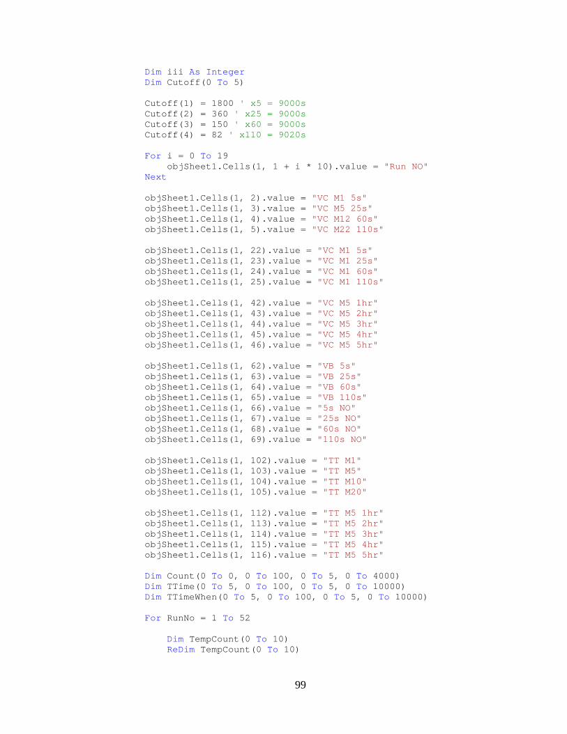
99
Dim iii As Integer Dim Cutoff(0 To 5) Cutoff(1) = 1800 ' x5 = 9000s Cutoff(2) = 360 ' x25 = 9000s Cutoff(3) = 150 ' x60 = 9000s Cutoff(4) = 82 ' x110 = 9020s For i = 0 To 19 objSheet1.Cells(1, 1 + i * 10).value = "Run NO" Next objSheet1.Cells(1, 2).value = "VC M1 5s" objSheet1.Cells(1, 3).value = "VC M5 25s" objSheet1.Cells(1, 4).value = "VC M12 60s" objSheet1.Cells(1, 5).value = "VC M22 110s" objSheet1.Cells(1, 22).value = "VC M1 5s" objSheet1.Cells(1, 23).value = "VC M1 25s" objSheet1.Cells(1, 24).value = "VC M1 60s" objSheet1.Cells(1, 25).value = "VC M1 110s" objSheet1.Cells(1, 42).value = "VC M5 1hr" objSheet1.Cells(1, 43).value = "VC M5 2hr" objSheet1.Cells(1, 44).value = "VC M5 3hr" objSheet1.Cells(1, 45).value = "VC M5 4hr" objSheet1.Cells(1, 46).value = "VC M5 5hr" objSheet1.Cells(1, 62).value = "VB 5s" objSheet1.Cells(1, 63).value = "VB 25s" objSheet1.Cells(1, 64).value = "VB 60s" objSheet1.Cells(1, 65).value = "VB 110s" objSheet1.Cells(1, 66).value = "5s NO" objSheet1.Cells(1, 67).value = "25s NO" objSheet1.Cells(1, 68).value = "60s NO" objSheet1.Cells(1, 69).value = "110s NO" objSheet1.Cells(1, 102).value = "TT M1" objSheet1.Cells(1, 103).value = "TT M5" objSheet1.Cells(1, 104).value = "TT M10" objSheet1.Cells(1, 105).value = "TT M20" objSheet1.Cells(1, 112).value = "TT M5 1hr" objSheet1.Cells(1, 113).value = "TT M5 2hr" objSheet1.Cells(1, 114).value = "TT M5 3hr" objSheet1.Cells(1, 115).value = "TT M5 4hr" objSheet1.Cells(1, 116).value = "TT M5 5hr" Dim Count(0 To 0, 0 To 100, 0 To 5, 0 To 4000) Dim TTime(0 To 5, 0 To 100, 0 To 5, 0 To 10000) Dim TTimeWhen(0 To 5, 0 To 100, 0 To 5, 0 To 10000) For RunNo = 1 To 52 Dim TempCount(0 To 10) ReDim TempCount(0 To 10)

100
Console.WriteLine(RunNo & " start " & Now()) For i = 0 To 19 objSheet1.Cells(1 + (RunNo), 1 + i * 10).value = RunNo Next 'read from excel For i = 1 To 3599 Count(0, RunNo, 1, i) = objSheet2.C ells(2 + i + (RunNo - 1) * 4000, 3).value For ii = 1 To 1 ''''''''''''''''''''''''''' total route number If objSheet2.Cells(2 + i + (RunNo - 1) * 4000, 30 + 26 * ii).value > 0 Then For iii = 1 To objSheet2.Cells(2 + i + (RunNo - 1) * 4000, 56).value TempCount(ii) = TempCou nt(ii) + 1 TTime(ii, RunNo, 1, Tem pCount(ii)) = objSheet2.Cells(2 + i + (RunNo - 1) * 4000, 55).val ue 'travel time TTimeWhen(ii, RunNo, 1, TempCount(ii)) = i * 5 'simulation time objSheet1.Cells(TempCou nt(ii) + 150, 1) = TempCount(ii) objSheet1.Cells(TempCou nt(ii) + 150, RunNo * 2) = TTime(ii, RunNo, 1, TempCount(ii)) objSheet1.Cells(TempCou nt(ii) + 150, RunNo * 2 + 1) = TTimeWhen(ii, RunNo, 1, TempCount(ii)) Next End If Next Next Dim IntCount(0 To 10) IntCount(1) = 1 IntCount(2) = 5 IntCount(3) = 12 IntCount(4) = 22 Dim Temp0 As Integer For Temp0 = 2 To 4 Interval = IntCount(Temp0) For i = 1 To Int(3599 / Interval) Dim Temp1 As Single = 0 Dim Temp2 As Single = 0 For iii = 1 To Interval Temp1 = Temp1 + Count(0, Ru nNo, 1, (i - 1) * Interval + iii) Next Count(0, RunNo, Temp0, i) = Tem p1 / Interval Next Next
101
objSheet1.Cells(RunNo + 1, 7) = Count(0 , RunNo, 1, 3599) Dim IntTT(0 To 10) IntTT(1) = 1 IntTT(2) = 5 IntTT(3) = 10 IntTT(4) = 20 For Temp0 = 2 To 4 Interval = IntTT(Temp0) For ii = 1 To 1 For i = 1 To Int(TempCount(ii) / Interval) Dim Temp3 As Single = 0 For iii = 1 To Interval Temp3 = Temp3 + TTime(i i, RunNo, 1, (i - 1) * Interval + iii) Next TTime(ii, RunNo, Temp0, i) = Temp3 / Interval TTimeWhen(ii, RunNo, Temp0, i) = TTimeWhen(ii, RunNo, 1, i * Interval) Next Next Next For Temp0 = 1 To 4 Interval = IntCount(Temp0) Dim CountTerm1(0 To Int(3599 / Interval)) As Single Dim CountTerm2(0 To Int(3599 / Interval)) As Single ReDim CountTerm1(0 To Int(3599 / Interval)) ReDim CountTerm2(0 To Int(3599 / Interval)) For i = 0 To Int(3599 / Interval) - 1 Dim Temp4 As Single = 0 Dim Temp5 As Single = 0 Dim Temp6 As Single = 0 Dim Temp7 As Single = 0 Dim Temp8 As Single = 0 For ii = 1 To Int(3599 / Interval) - 1 - i + 1 Temp4 = Temp4 + Count(0, Ru nNo, Temp0, i + ii) Temp6 = Temp6 + 1 Next CountTerm1(i) = Temp4 / Temp6 For iii = i + 1 To Int(3599 / Interval) Temp7 = Temp7 + (Count(0, R unNo, Temp0, iii) - CountTerm1(i)) * (Count(0, RunNo, Temp0, iii) - Cou ntTerm1(i)) Next CountTerm2(i) = Temp7 / (Int(35 99 / Interval) - i) / (Int(3599 / Interval) - i)

102
Next Dim Temp9 As Single = CountTerm2(1) Dim Temp10 As Single = Interval * 5 For i = 1 To Int(3599 / Interval) - 1 - Cutoff(Temp0) If CountTerm2(i) < Temp9 Then Temp9 = CountTerm2(i) Temp10 = i * Interval * 5 End If Next objSheet1.Cells(RunNo + 1, Temp0 + 1) = Temp10 Next For Temp0 = 1 To 4 Interval = IntCount(Temp0) Dim CountTerm1(0 To Int(3599 / Interval)) As Single Dim CountTerm2(0 To Int(3599 / Interval)) As Single ReDim CountTerm1(0 To Int(3599 / Interval)) ReDim CountTerm2(0 To Int(3599 / Interval)) For i = 0 To Int(3599 / Interval) - 1 ' 0 <= d < n Dim Temp4 As Single = 0 Dim Temp5 As Single = 0 Dim Temp6 As Single = 0 Dim Temp7 As Single = 0 Dim Temp8 As Single = 0 For ii = 1 To Int(3599 / Interval) - 1 - i + 1 Temp4 = Temp4 + Count(0, Ru nNo, 1, i * Interval + ii * Interval) Temp6 = Temp6 + 1 Next CountTerm1(i) = Temp4 / Temp6 For iii = i + 1 To Int(3599 / Interval) Temp7 = Temp7 + (Count(0, R unNo, Temp0, iii) - CountTerm1(i)) * (Count(0, RunNo, Temp0, iii) - Cou ntTerm1(i)) Next CountTerm2(i) = Temp7 / (Int(35 99 / Interval) - i) / (Int(3599 / Interval) - i) Next Dim Temp9 As Single = CountTerm2(1) Dim Temp10 As Single = Interval * 5 Dim Temp12 As Single = Interval * 5 For i = 1 To Int(3599 / Interval) - 1 - Cutoff(Temp0) If CountTerm2(i) < Temp9 Then Temp9 = CountTerm2(i) Temp10 = i * Interval * 5 End If

103
Next objSheet1.Cells(RunNo + 1, Temp0 + 21) = Temp10 Next Dim RunLength(0 To 10) RunLength(1) = 144 '144 x 25 = 3600s or 1hr RunLength(2) = 288 '288 x 25 = 7200s or 2hr RunLength(3) = 432 '432 x 25 = 10800s or 3hr RunLength(4) = 576 '576 x 25 = 14400s or 4hr RunLength(5) = 720 '720 x 25 = 18000s or 5hr For Temp0 = 1 To 5 Dim Length As Integer Length = RunLength(Temp0) Dim CountTerm1(0 To Length) As Single Dim CountTerm2(0 To Length) As Single ReDim CountTerm1(0 To Length) ReDim CountTerm2(0 To Length) For i = 0 To Length - 1 Dim Temp4 As Single = 0 Dim Temp5 As Single = 0 Dim Temp6 As Single = 0 Dim Temp7 As Single = 0 Dim Temp8 As Single = 0 For ii = 1 To Length - 1 - i + 1 Temp4 = Temp4 + Count(0, Ru nNo, 2, i + ii) Temp6 = Temp6 + 1 Next CountTerm1(i) = Temp4 / Temp6 For iii = i + 1 To Length Temp7 = Temp7 + (Count(0, R unNo, 2, iii) - CountTerm1(i)) * (Count(0, RunNo, 2, iii) - CountTe rm1(i)) Next CountTerm2(i) = Temp7 / (Length - i) / (Length - i) Next Dim Temp9 As Single = CountTerm2(1) Dim Temp10 As Single = 25 For i = 1 To Length - 1 - Cutoff(2) If CountTerm2(i) < Temp9 Then Temp9 = CountTerm2(i) Temp10 = i * 25 End If
104
Next objSheet1.Cells(RunNo + 1, Temp0 + 41) = Temp10 Next 'Volume Balancing with different interval For Temp0 = 1 To 4 Interval = IntCount(Temp0) Dim Temp4 As Single = 0 Dim Temp5 As Single = 0 Dim Temp6 As Single = 0 Dim Temp7 As Integer = 0 For i = 3 To Int(3599 / Interval) - 1 Temp4 = Count(0, RunNo, 1, Inte rval * (i - 2)) Temp5 = Count(0, RunNo, 1, Inte rval * (i - 1)) Temp6 = Count(0, RunNo, 1, Inte rval * (i - 0)) If (Abs(Temp4 - Temp5) / Temp4) < 0.12 And (Abs(Temp5 - Temp6) / Temp5) < 0.08 Then Temp7 = Temp7 + 1 If Temp7 = 1 Then objSheet1.Cells(RunNo + 1, Temp0 + 61) = i * Interval * 5 End If End If Next Next 'Travel Time MSER with different batch sizes For Temp0 = 1 To 4 Interval = IntTT(Temp0) Dim TTTerm1(0 To Int(TempCount(1) / Interval)) As Single Dim TTTerm2(0 To Int(TempCount(1) / Interval)) As Single ReDim TTTerm1(0 To Int(TempCount(1) / Interval)) ReDim TTTerm2(0 To Int(TempCount(1) / Interval)) For i = 0 To Int(TempCount(1) / Interval) - 1 ' 0 <= d < n Dim Temp4 As Single = 0 Dim Temp5 As Single = 0 Dim Temp6 As Single = 0 Dim Temp7 As Single = 0 Dim Temp8 As Single = 0 For ii = 1 To Int(TempCount(1) / Interval) - 1 - i + 1 Temp4 = Temp4 + TTime(1, Ru nNo, Temp0, i + ii) Temp6 = Temp6 + 1 Next TTTerm1(i) = Temp4 / Temp6

105
For iii = i + 1 To Int(TempCount(1) / Interval) Temp7 = Temp7 + (TTime(1, R unNo, Temp0, iii) - TTTerm1(i)) * (TTime(1, RunNo, Temp0, iii) - TTTerm 1(i)) Next TTTerm2(i) = Temp7 / (Int(TempC ount(1) / Interval) - i) / (Int(TempCount(1) / Interval) - i) Next 'Find the minimum value Dim Temp9 As Single = TTTerm2(1) Dim Temp10 As Single = TTimeWhen(1, RunNo, Temp0, 1) For i = 1 To Int(TempCount(1) / Interval) - 1 - Cutoff(Temp0) If TTTerm2(i) < Temp9 Then Temp9 = TTTerm2(i) Temp10 = TTimeWhen(1, RunNo , Temp0, i) End If Next objSheet1.Cells(RunNo + 1, Temp0 + 101) = Temp10 Next 'Travel Time MSER5 with different run lengths For i = 1 To Int(TempCount(1) / 5) If TTimeWhen(1, RunNo, 2, i) <= 3600 Then RunLength(1) = i ElseIf TTimeWhen(1, RunNo, 2, i) <= 7200 Then RunLength(2) = i ElseIf TTimeWhen(1, RunNo, 2, i) <= 10800 Then RunLength(3) = i ElseIf TTimeWhen(1, RunNo, 2, i) <= 14400 Then RunLength(4) = i End If RunLength(5) = Int(TempCount(1) / 5 ) Next For Temp0 = 1 To 5 Dim Length As Integer Length = RunLength(Temp0) Dim TTimeTerm1(0 To Length) As Single Dim TTimeTerm2(0 To Length) As Single ReDim TTimeTerm1(0 To Length) ReDim TTimeTerm2(0 To Length) For i = 0 To Length - 1 ' 0 <= d < n Dim Temp4 As Single = 0 Dim Temp5 As Single = 0 Dim Temp6 As Single = 0 Dim Temp7 As Single = 0 Dim Temp8 As Single = 0 For ii = 1 To Length - 1 - i + 1 Temp4 = Temp4 + TTime(1, Ru nNo, 2, i + ii)

106
Temp6 = Temp6 + 1 Next TTimeTerm1(i) = Temp4 / Temp6 For iii = i + 1 To Length Temp7 = Temp7 + (TTime(1, R unNo, 2, iii) - TTimeTerm1(i)) * (TTime(1, RunNo, 2, iii) - TTimeTe rm1(i)) Next TTimeTerm2(i) = Temp7 / (Length - i) / (Length - i) Next 'Finding the minimum value Dim Temp9 As Single = TTimeTerm2(1) Dim Temp10 As Single = TTimeWhen(1, RunNo, 2, 1) For i = 1 To Length - 1 - Cutoff(2) If TTimeTerm2(i) < Temp9 Then Temp9 = TTimeTerm2(i) Temp10 = TTimeWhen(1, RunNo , 2, i) End If Next objSheet1.Cells(RunNo + 1, Temp0 + 111) = Temp10 Next Next Console.WriteLine(Abs(DateDiff(DateInterval .Second, Start, Now())) & " " ) End Sub End Class

107
REFERENCES
1. Ni, D. A Framework for New Generation Transportation Simulation. in 2006 Winter Simulation Conference. 2006. Monterey, CA: IEEE.
2. Grassmann, W.K., Warm-up Periods in Simulation can be Detrimental. Probability in Engineering and Informational Sciences, 2008. 22(3): p. 415-429.
3. Law, A.M. and W.D. Kelton, Simulation Modeling and Analysis. Third ed, ed. K.E. Case and P.M. Wolfe. 2000, Boston: McGraw-Hill Series in Industrial Engineering and Management Science.
4. Sandikçi, B. and I. Sabuncuoglu, Analysis of the behavior of the transient period in non-terminating simulations. European Journal of Operational Research, 2006. 173(1): p. 252-267.
5. Robinson, S. Automated Analysis of Simulation Output Data. in 2005 Winter Simulation Conference. 2005. Orlando, FL.
6. Law, A.M. and W.D. Kelton, Simulation Modeling and Analysis. Fourth ed, ed. K.E. Case and P.M. Wolfe. 2007, New York: McGraw-Hill Series in Industrial Engineering and Management Science.
7. PTV, VISSIM 5.10 User Manual. 2008, Planung Transport Verkehr AG: Karlsruhe, Germany.
8. Fishman, G.S., Discrete-event Simulation: Modeling, Programming, And Analysis. Springer Series in Operations Research. 2001, New York: Springer.
9. Banks, J., I. Carson, John S., and B.L. Nelson, Discrete-Event System Simulation. Second ed. 1996, Upper Saddle River, NJ: Prentice-Hall Inc.
10. Robinson, S., A Statistical Process Control Approach to Selecting a Warm-up Period for Discrete-event Simulation. European Journal of Operational Research, 2007. 176(1): p. 332-346.

108
11. Bause, F. and M. Eickhoff. Truncation Point Estimation Using Multiple Replications in Parallel. in 2003 Winter Simulation Conference. 2003. New Orleans, LA: IEEE.
12. Welch, P.D., The Statistical Analysis of Simulation Results. Computer Performance Modeling Handbook, ed. S.S. Lavenberg. 1983, New York: Academic Press, Inc.
13. White, J., K. Preston, An Effective Truncation Heuristic for Bias Reduction in Simulation Output. Simulation, 1997. 69(6): p. 323-334.
14. White, J., K. Preston, M.J. Cobb, and S.C. Spratt. A Comparison of Five Steady-State Truncation Heuristics for Simulation. in 2000 Winter Simulation Conference. 2000. Orlando, FL.
15. Mokashi, A.C., et al. Performance Comparison of MSER-5 and N-Skart on the Simulation Start-up Problem. in 2010 Winter Simulation Conference. 2010. Baltimore, MD.
16. Conway, R.W., Some Tactical Problems in Digital Simulation. Management Science, 1963. 10(1): p. 47-61.
17. Mahajan, P.S. and R.G. Ingalls. Evaluation of Methods Used to Detect Warm-up Period in Steady State Simulation. in 2004 Winter Simulation Conference. 2004. Washington, DC.
18. Gafarian, A.V., C.J. Ancker, and T. Morisaku, Evaluation of commonly used rules for detecting steady-state in computer simulation. Naval Research Logistics Quarterly, 1978. 25: p. 511-529.
19. Alexopoulos, C., S. Andradottir, and N.T. Argon. Replicated Batch Means for Steady-State Simulations with Initial Transients. in 2007 Winter Simulation Conference. 2007. Washington, DC: IEEE.
20. Argon, N.T. and S. Andradottir, Replicated batch means for steady-state simulations. Naval Research Logistics, 2006. 53(6): p. 508-524.
21. Yücesan, E., Randomization tests for initialization bias in simulation output. Naval Research Logistics, 1993. 40(5): p. 643-663.

109
22. Kelton, W.D. and A.M. Law, A new approach for dealing with the startup problem in discrete event simulation. Naval Research Logistics Quarterly, 1983. 30: p. 641-658.
23. Hoad, K., S. Robinson, and R. Davies. Automating Warm-Up Length Estimation. in 2008 Winter Simulation Conference. 2008. Miami, FL.
24. Steiger, N.M., et al. Steady-state Simulation Analysis using ASAP3. in 2004 Winter Simulation Conference. 2004. Washington, DC.
25. Holm, P., et al., Traffic Analysis Toolbox Volume IV: Guidelines for Applying CORSIM Microsimulation Modeling Software, FHWA, Editor. 2007. p. 201-204.
26. Franklin, W.W. and J. White, K. Preston. Stationarity Tests and MSER-5: Exploring the Intuition Behind Mean-Square-Error-Reduction in Detecting and Correcting Initialization Bias. in 2008 Winter Simulation Conference. 2008. Miami, FL: IEEE.
27. Google, Google Earth. 2010, Google, Inc.: Mountain View, CA.
Top Related