


Languages
Pages
Legal


�
�������������������������� �������������������������������������������������������
�������������������������������������
���������������������������������������������
������ �� ��� ���� ����� ��������� ����� �������� ���� ��� � ��� ���� ��������
���������������� �������������������������������������������������
�������������������������������������������������
����������������� ��
�
�
�
�
������������ ���
an author's https://oatao.univ-toulouse.fr/20436
Paroissien, Eric and Silva, Lucas Filipe Martins da and Lachaud, Frédéric Simplified stress analysis of functionally
graded single-lap joints subjected to combined thermal and mechanical loads. (2018) Composite Structures, 203.
ISSN 0263-8223

1
Simplified stress analysis of functionally graded single-lap joints subjected to combined
thermal and mechanical loads
Eric Paroissien1,*
, Lucas FM da Silva2, Frédéric Lachaud
1
1 Institut Clément Ader (ICA), Université de Toulouse, ISAE-SUPAERO, INSA, IMT MINES
ALBI, UTIII, CNRS, 3 Rue Caroline Aigle, 31400 Toulouse, France
2 Department of Mechanical Engineering, Faculty of Engineering, University of Porto,
Portugal
*To whom correspondence should be addressed: Tel. +33561338438, E-mail:
Abstract – Functionally graded adhesive (FGA) joints involve a continuous variation of the
adhesive properties along the overlap allowing for the homogenization of the stress
distribution and load transfer, in order to increase the joint strength. The use of FGA joints
made of dissimilar adherends under combined mechanical and thermal loads could then be an
attractive solution. This paper aims at presenting a 1D-bar and a 1D-beam simplified stress
analyses of such multimaterial joints, in order to predict the adhesive stress distribution along
the overlap, as a function of the adhesive graduation. The graduation of the adhesive
properties leads to differential equations which coefficients can vary the overlap length. For
the 1D-bar analyses, two different resolution schemes are employed. The first one makes use
of Taylor expansion power series (TEPS) as already published under pure mechanical load.
The second one is based on the macro-element (ME) technique. For the 1D-beam analysis, the
solution is only based on the ME technique. A comparative study against balanced and

2
unbalanced joint configurations under pure mechanical and/or thermal loads involving
constant or graduated adhesive properties are provided to assess the presented stress analyses.
The mathematical description of the analyses is provided.
Key words: functionally graded adhesive; single-lap bonded joint; stress analysis; macro-
element; thermoelasticity; dissimilar adherend.

3
NOMENCLATURE AND UNITS
Aj extensional stiffness (N) of adherend j
Bj extensional and bending coupling stiffness (N.mm) of adherend j
Dj bending stiffness (N.mm2) of adherend j
Ea adhesive peel modulus (MPa)
Ea,min adhesive shear modulus (MPa)
Ea,max adhesive shear modulus (MPa)
Ej adherend Young’s modulus (MPa) of adherend j
F magnitude of applied force (N)
Fe element nodal force vector
Fe,therm element nodal force vector equivalent to thermal load
Ga adhesive shear modulus (MPa)
Ga,max maximal adhesive shear modulus (MPa)
Ga,min minimal adhesive shear modulus (MPa)
KBBa elementary stiffness matrix of a bonded-bars element
KBBe elementary stiffness matrix of a bonded-beams element
Kbar,j elementary stiffness matrix of a bar for the adherend j
L length (mm) of bonded overlap
Me element matrix linking the element nodal displacement to the constant integration
vector
Mj bending moment (N.mm) in adherend j around the z direction
Me element matrix linking the element nodal force to the constant integration vector
𝑀𝑗Δ𝑇 thermal bending moment (N.mm) in adherend j around the z direction
Nj normal force (N) in adherend j in the x direction
𝑁𝑗Δ𝑇 thermal normal force (N) in adherend j in the x direction
4
S adhesive peel stress (MPa)
T adhesive shear stress (MPa)
Tmax maximal adhesive shear stress (MPa)
Ue element nodal displacement vector
Vj shear force (N) in adherend j in the y direction
b width (mm) of the adherends
c half-length (mm) of bonded overlap
ea thickness (mm) of the adhesive layer
hj half thickness (mm) of adherend j
kI adhesive elastic stiffness (MPa/mm) in peel
kII adhesive elastic stiffness (MPa/mm) in shear
n_max order of truncation
n_ME number of macro-elements
p power of the graduation law
uj displacement (mm) of adherend j in the x direction
vj displacement (mm) of adherend j in the y direction
overlap length (mm) of a macro-element
T variation of temperature (K)
u slipping displacement (mm)
j characteristic parameter (N2.mm
2) of adherend j
j coefficient of thermal expansion (K-1
) of adherend j
j bending angle (rad) of the adherend j around the z direction
𝜒𝐴 adherend stiffness unbalance parameter (-)
𝜒𝛼 adherend thermal unbalance parameter (-)
(X,Y,Z) element reference system of axes

5
(x,y,z) global reference system of axes
BBa Bonded-bars
BBE Bonded-beams
CTE coefficient of thermal expansion
FE Finite Element
FGA functionally graded adhesive
GM general model
ISLM improved shear-lap model
JE joint element
ME macro-element
ODE ordinary differential equation
TC test case
TEPS Taylor expansion in power series

6
1. Introduction
In the frame of structural design, the proper choice of joining technology is decisive for the
integrity of the manufactured structure. Mechanical fastening, such as riveting or screwing,
appears to be a reliable solution for the designers. Nevertheless, alone or in combination with
mechanical fastening, the adhesive bonding technology may offer significantly improved
mechanical performance in terms of stiffness, static strength and fatigue strength [1-3].
Indeed, unlike the discrete load transfer of mechanical fasteners, the load transfer between
structural bonded components is continuous all along the overlap. This higher level of
mechanical performance allows for lighter joints. In other words, adhesive bonding offers the
possibility to reduce the structural mass while ensuring the mechanical strength. The
optimization of the strength-to-weight ratio is a challenge for several industrial sectors, such
as aerospace, automotive, rail or naval transport industries.
Nevertheless, stress gradients at both overlap ends appear in bonded joints, due to the relative
deformation of the adhesive layer with regards to the adherends. It leads to a load transfer
restricted on a small length at the overlap ends. In order to increase the load capability of
bonded joints, the reduction of adhesive peak stresses is wanted. The specimen design for the
thick adherend shear test [4] leads to both a homogenization of the adhesive shear stress and
a drastic reduction the adhesive peel stress, all the more when care is taken to reduce the edge
effects [5]. Another approach is to make the material and/or geometrical properties of the
adherends and/or the adhesive layer vary along the overlap. Several design solutions have
been published [3]. For example, a solution is the tapering of adherends at overlap ends,
which allows for a progressive increase of the neutral line lag and a reduction of adhesive peel
stress [6-7]. A more local solution is the rounding of adherend corner associated with
adhesive spew fillets [8-9]. The mixed adhesive solution which is a rough version of a graded
joint consists in the use of various different adhesives along the overlap to increase the joint

7
strength [10-13]. In recent past years, functionally graded adhesive (FGA) have been more
and more considered [14-15]. FGA joints involve a continuous variation of the adhesive
properties along the overlap allowing for the homogenization of the stress distribution and
load transfer. When dissimilar adherends have to be bonded, the adhesive stress distribution is
asymmetrical, so that one of the overlap ends is overstressed. Moreover, this overstressing is
magnified under thermal loads due to the mismatch in coefficient of thermal expansion (CTE)
of adherends. The capability of a local graduation of the adhesive stiffness is a promising
solution to optimize the strength of multimaterial joints under severe loads, such as combined
thermal and mechanical. This situation occurs very often in multi-material structures found in
the transport industry. That is why the development of dedicated stress analyses to predict the
stress distribution is fundamental. The Finite Element (FE) method is able to address the
stress analysis of FGA joints [12,14]. Nevertheless, since analyses based on FE models are
computationally costly, it would be profitable both to restrict them to refined analyses and to
develop simplified approaches, enabling extensive parametric studies and optimization
processes. Moreover, numerous simplified stress analyses of bonded joints are available and
provide accurate predictions [16-18]. In 2014, Carbas et al. published a first analytical
approach for 1D-bar stress analysis of FGA joints [19]. This stress analysis is based on the
shear-lag approach by Volkersen [20] associated with a resolution scheme making use of
Taylor expansion in power series (TEPS) to solve the involved differential equations. This
stress analysis is restricted to half of the overlap length of balanced joints with a linear
graduation of the adhesive shear modulus. Stein et al. presented a 1D-bar analysis using TEPS
resolution able to address unbalanced bonded joints under any adhesive properties graduations
[21-22]. This analysis is called by the authors Improved Shear Lag Model (ISLM). Moreover,
Stein et al. provided a sandwich-type analysis using TEPS resolution, taking into accounts
both in-plane and out-of-plane load, termed General Model (GM). The sandwich-type

8
analysis concept comes from the analysis methodology by Goland and Reissner [23] who
provided the first closed-form solution for the adhesive stress distribution for simply
supported balanced joint made of adherends undergoing cylindrically bending. Goland and
Reissner took into account the geometrical non linearity due to the lag of neutral line to assess
the bending moment at both overlap ends through a bending moment factor. This
methodology was then employed by other researchers to improve the initial model [24-32]
leading to various forms of the bending moment factor [33]. In 2017, Stapleton et al. used a
joint element (JE) for the stress analysis of FGA joints under various geometrical
configurations, including in-plane and out-of-plane load as well as non-linear material
behavior [34]. A JE is a 4-nodes brick element allowing for the modelling of two bonded
adherends [34-35]. Over a similar period of time, the first and third authors of the present
papers and co-workers have been working on the development of the macro-element (ME)
technique for the simplified stress analysis of bonded, bolted and hybrid (bonded/bolted)
joints [36-43]. Dedicated 4-nodes Bonded-bars (BBa) and Bonded-beams (BBe) have been
formulated. As for the JE model, only one BBa or BBe, depending on the chosen kinematics,
is sufficient to be representative for an entire bonded overlap in the frame of a linear elastic
analysis (see Figure 1). When the geometrical or material properties of the adherends or the
adhesive layer vary along the overlap a mesh is necessary along the overlap length direction
only. The ME technique is inspired by the FE method and differs in the sense that the
interpolation functions are not assumed. Indeed, they take the shape of solutions of the
governing ordinary differential equations (ODEs) system, coming from the constitutive
equations of the adhesive and adherends and from the local equilibrium equations, related to
the simplifying hypotheses. The main work is thus the formulation of the elementary stiffness
matrix of the ME. Once the stiffness matrix of the complete structure is assembled from the
elementary matrices and the boundary conditions are applied, the minimization of the

9
potential energy provides the solution, in terms of adhesive stress distributions along the
overlap, internal forces and displacements in the adherends. The ME technique can be
regarded as mathematical procedure allowing for the resolution of the system of ODE, under a
less restricted application field of simplifying hypotheses, in terms of geometry, material
behaviours, kinematics, boundary conditions and loads.
Stress analyses of bonded joints under thermal loads can be found in the literature linked to
the aerospace [44] or to the emergence of the industry of electronic packaging [45-48].
However, to the best knowledge of authors, there is not any published stress analyses of FGA
joints under thermal load. The present paper aims at presenting simplified stress analysis of
FGA single-lap joints under combined mechanical and thermal loads. Under the 1D-bar
kinematics, the resolution scheme by TEPS and by ME is used. As the 1D-bar TEPS and ME
analyses provide the same predictions, the resolution scheme by ME under the 1D-beam
kinematics is employed only. Indeed, the ME technique offers the possibility to extend the
application field to analyses involving nonlinear material behaviors, various geometries and
various applied boundary conditions [39-43]. The developed stress analyses are then assessed
against reference stress analyses for bonded and FGA joints on several test cases. The three
stress analyses presented need dedicated computer codes, which are provided as
supplementary materials with the present papers. These codes run on the MATLAB
commercial software. Moreover, for the comfort of readers, this paper provides the useful
mathematical steps, even if some elements have eventually been published elsewhere.

10
Figure 1. Modelling of a bonded overlap by a macro-element.
2. Description of simplified stress analyses of FGA single-lap joints
2.1. Under 1D-bar kinematics
2.1.1 Hypotheses
The following hypotheses are taken (i) the adherends are linear elastic materials simulated as
bars, (ii) the adhesive layer is simulated by an infinite number of linear elastic shear springs
linking both adherends, and (iii) the shape of graduation of the adhesive layer shear modulus
is considered. As a result, it is supposed that all the adhesive stress components vanish except
the in-plane shear. The case of a single-lap joint subjected to combined mechanical and
thermal loads is considered. The geometrical parametrization is provided in Figure 2. The
subscript 1 (2) refers to the upper (lower) adherend. The origin of the global reference system
is taken at the centre of the overlap, with the x-axis along the overlap length direction, the
only axis according to which displacements u are possible. The joint is submitted to an
uniform variation of temperature T, to a tensile force F at one extremity and is fixed at the
other one. The stress analysis is conducted in force but could similarly be made in tensile flow
F/b.
bonded overlap
macro-element
neutral axis of adherend 1
neutral axis of adherend 2
adhesive layer

11
Figure 2. Geometrical parametrization of the single-lap joint, boundary conditions and applied
loads (1D-bar analysis).
2.1.2 Governing equations
The local equilibrium of both adherends (see Figure 3) provides the following equations:
𝑑𝑁𝑗
𝑏𝑑𝑥= (−1)𝑗𝑇(𝑥), 𝑗 = 1,2 (1)
where b is the overlap width, Nj the normal force in the adherend j and T the adhesive shear
stress.
Figure 3. Free body diagram of infinitesimal pieces included between x and x+dx of both
adherends in the overlap region. Subscript 1 (2) refers to the upper (lower) adherend.
The total strain is equal to the mechanical strain plus the thermal strain such as:
𝑑𝑢𝑗
𝑑𝑥=𝑁𝑗
𝐴𝑗+ 𝛼𝑗Δ𝑇 , 𝑗 = 1,2 (2)
where j is the coefficient of thermal expansion of the adherend j. Aj is the membrane
stiffness of the adherend j, given by:
𝐴𝑗 = 𝐸𝑗𝑏𝑒𝑗 (3)
F x,u
y
c=L/2 c=L/2
e1
e2
width: b T
ea
u=0
neutral lines
l2 l1
N1(x+dx) N1(x)
T.bdx
N2(x+dx) N2(x)

12
where ej is the thickness of the adherend j and Ej the Young’s modulus of the adherend. The
displacement uj(x) is the normal displacement of points located at the abscissa x on the neutral
line of adherend j (see Figure 2).
The constitutive equation for the adhesive layer is provided by:
𝑇 = 𝐺𝑎𝑢2−𝑢1
𝑒𝑎= 𝑘𝐼𝐼Δ𝑢 (4)
with:
Δ𝑢 = 𝑢2 − 𝑢1 (5)
where ea is the adhesive thickness, Ga the adhesive shear modulus and kII=Ga/ea the adhesive
shear relative stiffness. u is the differential displacement of the adherend interface. The
stress analyses presented use kII andu, so that they can be directly applied when the
thickness of the adhesive layer varies along the overlap.
2.1.3 TEPS resolution
The approach using TEPS resolution scheme is firstly used. The differentiation of Eq. (2) with
respect to x provides:
𝑑2𝑢𝑗
𝑑𝑥2=
1
𝐴𝑗
𝑑𝑁𝑗
𝑑𝑥, 𝑗 = 1,2 (6)
By using the local equilibrium equation Eq. (1) and the adhesive constitutive equation Eq. (4),
it comes:
𝑑2𝑢𝑗
𝑑𝑥2=
1
𝐴𝑗(−1)𝑗𝑏𝑇(𝑥) =
𝑏
𝐴𝑗(−1)𝑗𝑘𝐼𝐼Δ𝑢, 𝑗 = 1,2 (7)
As a result, a second order differential equation in the slipping displacement (relative
horizontal displacement of the interface) can be written:
𝑑²Δ𝑢
𝑑𝑥²− �̃�2𝑘𝐼𝐼Δ𝑢 = 0 (8)
with:

13
�̃�2 =1
𝑒1𝐸1+
1
𝑒2𝐸2=1+𝜒𝐴
𝐴′2 (9)
𝜒𝐴 =𝐴′2
𝐴′1=𝑒2𝐸2
𝑒1𝐸1=𝐴2
𝐴1 (10)
A’j is the membrane stiffness of the adherend j per unit of width. 𝜒𝐴 is representative for the
stiffness unbalance of the joint. The differential equation Eq. (8) is relevant to the one
obtained by Stein et al. for the ISLM – which does not consider any thermal load – but written
in slipping displacement instead of shear strain [22]. A solution is then searched for any x
included between –c and c under the shape of TESP:
Δ𝑢(𝑥) = ∑ 𝑢𝑛𝑥𝑛∞
𝑛=0 (11)
For the series terms to have the same unit as the function approximated, the following
variable change is made in the present analysis:
ζ =𝑥
𝑐 (12)
As result, the solution is searched for any X included between –1 and 1 under the shape:
Δ𝑢(𝑥) = ∑ 𝑢𝑛(𝑐ζ)𝑛∞
𝑛=0 = ∑ 𝑢𝑛𝑐𝑛ζ𝑛∞
𝑛=0 = ∑ 𝑈𝑛ζ𝑛∞
𝑛=0 (13)
with:
∀𝑛, 𝑈𝑛 = 𝑐𝑛𝑢𝑛 (14)
The mth
derivative of u is then assessed as follows
𝑑𝑚Δ𝑢
𝑑𝑥𝑚=
1
𝑐𝑚𝑑𝑚Δ𝑢
𝑑ζ2=
1
𝑐𝑚∑ ∏ (𝑛 + 𝑖)𝑚
𝑖=1 𝑈𝑛+2ζ𝑛∞
𝑛=0 (15)
The graduation of adhesive properties is then described under the shape of a TESP:
𝑘𝐼𝐼(ζ) = ∑ 𝐾𝑛ζ𝑛∞
𝑛=0 = ∑ 𝑘𝑛𝑥𝑛∞
𝑛=0 = 𝑘𝐼𝐼(ζ) (16)
with:
∀𝑛, 𝐾𝑛 = 𝑐𝑛𝑘𝑛 (17)
The expressions for u and kII are then replaced in the second order differential equation Eq.
(8) leading to:
∑ (𝑛 + 1)(𝑛 + 2)𝑈𝑛+2ζ𝑛∞
𝑛=0 − 𝑐2�̃�2∑ 𝑈𝑛𝑋𝑛∞
𝑛=0 ∑ 𝐾𝑙ζ𝑙∞
𝑙=0 = 0 (18)
14
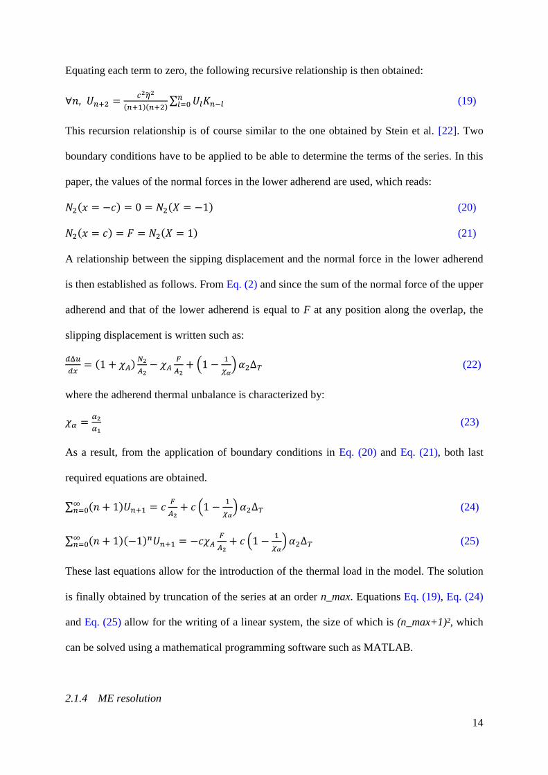
Equating each term to zero, the following recursive relationship is then obtained:
∀𝑛, 𝑈𝑛+2 =𝑐2�̃�2
(𝑛+1)(𝑛+2)∑ 𝑈𝑙𝐾𝑛−𝑙𝑛𝑙=0 (19)
This recursion relationship is of course similar to the one obtained by Stein et al. [22]. Two
boundary conditions have to be applied to be able to determine the terms of the series. In this
paper, the values of the normal forces in the lower adherend are used, which reads:
𝑁2(𝑥 = −𝑐) = 0 = 𝑁2(𝑋 = −1) (20)
𝑁2(𝑥 = 𝑐) = 𝐹 = 𝑁2(𝑋 = 1) (21)
A relationship between the sipping displacement and the normal force in the lower adherend
is then established as follows. From Eq. (2) and since the sum of the normal force of the upper
adherend and that of the lower adherend is equal to F at any position along the overlap, the
slipping displacement is written such as:
𝑑Δ𝑢
𝑑𝑥= (1 + 𝜒𝐴)
𝑁2
𝐴2− 𝜒𝐴
𝐹
𝐴2+ (1 −
1
𝜒𝛼)𝛼2Δ𝑇 (22)
where the adherend thermal unbalance is characterized by:
𝜒𝛼 =𝛼2
𝛼1 (23)
As a result, from the application of boundary conditions in Eq. (20) and Eq. (21), both last
required equations are obtained.
∑ (𝑛 + 1)𝑈𝑛+1∞𝑛=0 = 𝑐
𝐹
𝐴2+ 𝑐 (1 −
1
𝜒𝛼)𝛼2Δ𝑇 (24)
∑ (𝑛 + 1)(−1)𝑛𝑈𝑛+1∞𝑛=0 = −𝑐𝜒𝐴
𝐹
𝐴2+ 𝑐 (1 −
1
𝜒𝛼)𝛼2Δ𝑇 (25)
These last equations allow for the introduction of the thermal load in the model. The solution
is finally obtained by truncation of the series at an order n_max. Equations Eq. (19), Eq. (24)
and Eq. (25) allow for the writing of a linear system, the size of which is (n_max+1)², which
can be solved using a mathematical programming software such as MATLAB.
2.1.4 ME resolution

15
Firslty, the elementary stiffness matrix of a BBa element is formulated. The length of the BBa
is , on which the material and geometrical properties are supposed constant. The element
reference system of axis is denoted (X,Y,Z). The elementary stiffness matrix of the BBa,
termed KBBa, describes the interaction between the four nodal forces and the force nodal
displacements (see Figure 4), such as:
(
−𝑁1(0)
−𝑁2(0)
𝑁1(Δ)
𝑁2(Δ) )
= 𝐾𝐵𝐵𝑎
(
𝑢1(0)
𝑢2(0)
𝑢1(Δ)
𝑢2(Δ))
⟺ 𝐹𝑒 = 𝐾𝐵𝐵𝑎𝑈𝑒 (26)
where Fe (Ue) is the nodal force (displacement) vector of the BBa element.
Figure 4. Free body diagram of infinitesimal pieces included between x and x+dx of both
adherends in the overlap region. Subscript 1 (2) refers to the upper (lower) adherend.
In the frame of the 1D-bar analysis, the closed-form expressions for each component of KBBa
can be obtained [36-37]. Even if the mathematical description has already published under
another shape, it provided in Appendix A.
As expected, the obtained stiffness matrix is the same as the one obtained without considering
the thermal load. The method to take into account a linear variation of shear stress in the
adherend thickness following [28] is described in Appendix D.
Since the material properties of the adhesive vary along the overlap, the approach using the
ME technique consists in regularly meshing the overlap with BBa elements with n_ME BBa
elements (see Figure 5). Each BBa element has a length =L/n_ME, on which the material
X
node i
node j
node k
node l
u2(x)
u1(x) uk
ul
ui
uj
BBa
0 X
X
node i
node j
node k
node l N2(x)
N1(x)
Qk
Ql
Qi BBa
0 X
Qj
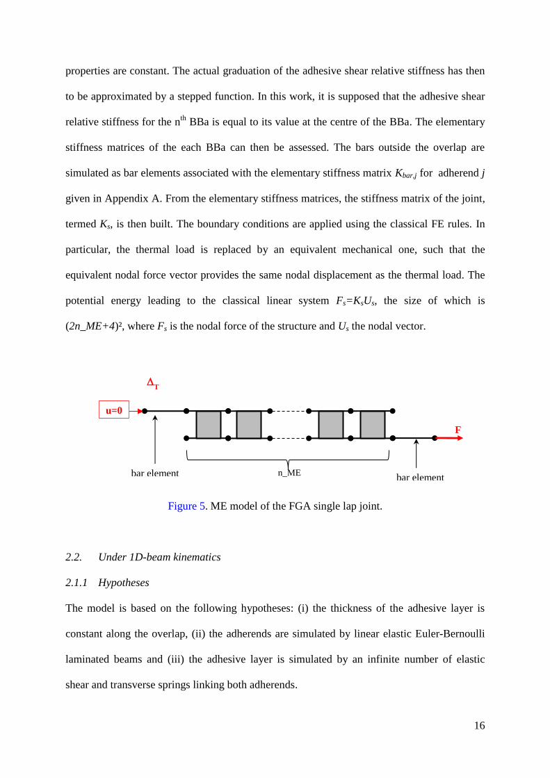
16
properties are constant. The actual graduation of the adhesive shear relative stiffness has then
to be approximated by a stepped function. In this work, it is supposed that the adhesive shear
relative stiffness for the nth
BBa is equal to its value at the centre of the BBa. The elementary
stiffness matrices of the each BBa can then be assessed. The bars outside the overlap are
simulated as bar elements associated with the elementary stiffness matrix Kbar,j for adherend j
given in Appendix A. From the elementary stiffness matrices, the stiffness matrix of the joint,
termed Ks, is then built. The boundary conditions are applied using the classical FE rules. In
particular, the thermal load is replaced by an equivalent mechanical one, such that the
equivalent nodal force vector provides the same nodal displacement as the thermal load. The
potential energy leading to the classical linear system Fs=KsUs, the size of which is
(2n_ME+4)², where Fs is the nodal force of the structure and Us the nodal vector.
Figure 5. ME model of the FGA single lap joint.
2.2. Under 1D-beam kinematics
2.1.1 Hypotheses
The model is based on the following hypotheses: (i) the thickness of the adhesive layer is
constant along the overlap, (ii) the adherends are simulated by linear elastic Euler-Bernoulli
laminated beams and (iii) the adhesive layer is simulated by an infinite number of elastic
shear and transverse springs linking both adherends.
n_ME
u=0
F
T
bar element bar element

17
Similarly to the 1D-bar analysis, the case of a single-lap joint subjected to combined
mechanical and thermal loads is considered, for which the geometrical parametrization is
provided in Figure 6. The joint is simply supported at both extremities and submitted to a
uniform variation of temperature T and to a tensile force F. It is indicated that any boundary
conditions could be applied when the ME technique is applied, even if simply supported is
chosen in this paper. The stress analysis is conducted in force but could similarly be made in
tensile flow F/b.
Figure 6. Geometrical parametrization of the single-lap joint, boundary condition and applied
loads (1D-beam analysis).
2.2.2 Governing Equation
The local equilibrium selected for the formulation of the presented BBe element is related to
the one used by Luo and Tong [31] and allows for a coupling between the in-plane and out-of-
plane load. Moreover, the formulation presented can be easily modified to correspond to the
Goland and Reissner [23] or to the Hart-Smith [24] local equilibrium.
The local equilibrium of both adherends (see Figure 7) provides the six following equations:
𝑑𝑁𝑗
𝑑𝑋= (−1)𝑗 cos 𝜃𝑗 𝑏𝑇, 𝑗 = 1,2 (27)
𝑑𝑉𝑗
𝑑𝑋= (−1)𝑗+1𝑏𝑆 + (−1)𝑗 sin 𝜃𝑗 𝑏𝑇, 𝑗 = 1,2 (28)
𝑑𝑀𝑗
𝑑𝑋+ 𝑉𝑗 + cos 𝜃𝑗 𝑏 (ℎ𝑗 +
𝑒𝑎
2)𝑇 − sin 𝜃𝑗 𝑁𝑗 = 0, 𝑗 = 1,2 (29)
F x,u
y,v
c=L/2 c=L/2
e1
e2
width: b T
ea
u=0
v=0
neutral lines
l2 l1
+,
v=0

18
with:
ℎ𝑗 =𝑒𝑗
2, 𝑗 = 1,2 (30)
where Vj is the shear force in the adherend j, Mj the bending moment in the adherend j, j the
bending angle in the adherend j and S is the adhesive peel stress.
Figure 7. Free body diagram of infinitesimal pieces included between x and x+dx of both
adherends in the overlap region. Subscript 1 (2) refers to the upper (lower) adherend.
The constitutive equations can then be written as:
𝑁𝑗 = 𝐴𝑗𝑑𝑢𝑗
𝑑𝑋− 𝐵𝑗
𝑑𝜃𝑗
𝑑𝑋− 𝑁𝑗
Δ𝑇 , 𝑗 = 1,2 (31)
𝑀𝑗 = −𝐵𝑗𝑑𝑢𝑗
𝑑𝑋+ 𝐷𝑗
𝑑𝜃𝑗
𝑑𝑋+𝑀𝑗
Δ𝑇 , 𝑗 = 1,2 (32)
𝜃𝑗 =𝑑𝑣𝑗
𝑑𝑋 (33)
where (see Appendix A) Aj is the membrane stiffness of adherend j, Bj the coupling
membrane-bending stiffness of adherend j, Dj the bending stiffness of adherend j, 𝑁𝑗Δ𝑇 the
X
Y +
N1+dN1
M1+dM1 V1+dV1
V2+dV2
N2+dN2
M2+dM2
M1
V1
V2 M2
N1
N2
S.bdx
T.bdx
T.bdx
1
1
2
1
ea/2

19
thermal normal force in the adherend j and 𝑀𝑗Δ𝑇 is the thermal bending moment in the
adherend j. In the case of a lay-up characterized by a mirror symmetry, Bj=0 and 𝑀𝑗Δ𝑇 = 0.
The constitutive equations for the adhesive layer are provided by:
𝑆 =𝐸𝑎
𝑒𝑎[𝑣1 − 𝑣2] = 𝑘𝐼Δ𝑣 (34)
𝑇 =𝐺𝑎
𝑒𝑎[𝑢2 − ℎ2𝜃2 − (𝑢1 + ℎ1𝜃1)] = 𝑘𝐼𝐼Δ𝑢 (35)
with:
Δ𝑢 = 𝑢2 − 𝑢1 − ℎ2𝜃2 − ℎ1𝜃1 (36)
Δ𝑣 = 𝑣1 − 𝑣2 (37)
where Ea is the adhesive peel modulus and kI=Ea/ea the adhesive peel relative stiffness. v is
representative of the opening displacement of the adherend interface. Contrary to the 1D-bar
analysis, the presented analysis cannot be directly applied when the thickness of the adhesive
layer varies along the overlap. Indeed, the variation of the thickness induces a lag of the
neutral axis, which has to be taken into account because of the deflection. Nevertheless, it is
indicated that the variation of the adhesive thickness could be easily taken into account when
using the ME technique.
2.2.3 ME resolution
The resolution scheme follows the same part as for the 1D-bar analysis (see section 2.1.4).
The single-lap joint is meshed in BBe elements along the overlap and beam elements for the
parts outside the overlap. The boundary conditions, the mechanical and thermal loads are then
applied. Similarly to the 1D-bar analysis, the thermal load is applied under the shape of an
equivalent nodal force vector given by:
20
𝐹𝑡ℎ =
(
−𝑁1Δ𝑇
−𝑁2Δ𝑇
𝑁1Δ𝑇
𝑁2Δ𝑇
0000
𝑀1Δ𝑇
𝑀2Δ𝑇
−𝑀1Δ𝑇
−𝑀2Δ𝑇)
(38)
Contrary to the 1D-bar analysis, it is not possible to simply obtain closed-form expressions for
the components of the stiffness matrix of the BBe element. An approach for the formulation
of the stiffness matrix of BBe element under Goland and Reissner equilibrium has already
been described in detail in previous papers [36-43]. Nevertheless, this approach could be long
to set up. In this paper, a new approach is provided for a fast and easy implementation within
mathematical software such as MATLAB for example. The present formulation ME has never
been published. The element reference system (X,Y,Z) of axes is considered. Following Luo
and Tong approach [31], a first approximation is made. The bending angle is supposed very
small. The six local equilibrium equations become then:
𝑑𝑁𝑗
𝑑𝑋= (−1)𝑗𝑏𝑇, 𝑗 = 1,2 (39)
𝑑𝑉𝑗
𝑑𝑋= (−1)𝑗+1𝑏𝑆 + (−1)𝑗𝜃𝑗𝑏𝑇, 𝑗 = 1,2 (40)
𝑑𝑀𝑗
𝑑𝑋+ 𝑉𝑗 + 𝑏 (ℎ𝑗 +
𝑒𝑎
2)𝑇 − 𝜃𝑗𝑁𝑗 = 0, 𝑗 = 1,2 (41)
A second approximation is made. It consists in neglecting the product of the adhesive shear
stress with the bending angle 𝑇𝜃𝑗 ≪ 1, 𝑗 = 1,2. The six local equilibrium equations become
then:
𝑑𝑁𝑗
𝑑𝑋= (−1)𝑗𝑏𝑇, 𝑗 = 1,2 (42)

21
𝑑𝑉𝑗
𝑑𝑋= (−1)𝑗+1𝑏𝑆, 𝑗 = 1,2 (43)
𝑑𝑀𝑗
𝑑𝑋+ 𝑉𝑗 + 𝑏 (ℎ𝑗 +
𝑒𝑎
2)𝑇 − 𝜃𝑗𝑁𝑗 = 0, 𝑗 = 1,2 (44)
Compared to the local equilibrium by Hart-Smith [24] only the bending moment is modified,
involving a coupling between normal forces and bending moment. The following quotation is
introduced for any functions f:
(𝑓+𝑓−) = (
1 11 −1
) (𝑓1𝑓2) (45)
A third and last approximation is made which reads 𝑁−
2(𝜃1 ∓ 𝜃2) ≪ 1. Under this
approximation and taking into account that the sum of normal forces at any abscissa is equal
to the applied force F, a system of twelve first order linear ODEs is obtained:
𝑑𝑢+
𝑑𝑋=1
2(𝐷1
Δ1+𝐷2
Δ2)𝑁+ +
1
2(𝐷1
Δ1−𝐷2
Δ2)𝑁− +
1
2(𝐵1
Δ1+𝐵2
Δ2)𝑀+ +
1
2(𝐵1
Δ1−𝐵2
Δ2)𝑀− (46)
𝑑𝑣+
𝑑𝑋= 𝜃+ (47)
𝑑𝜃+
𝑑𝑋=1
2(𝐵1
Δ1+𝐵2
Δ2)𝑁+ +
1
2(𝐵1
Δ1−𝐵2
Δ2)𝑁− +
1
2(𝐴1
Δ1+𝐴2
Δ2)𝑀+ +
1
2(𝐴1
Δ1−𝐴2
Δ2)𝑀− (48)
𝑑𝑢−
𝑑𝑋=1
2(𝐷1
Δ1−𝐷2
Δ2)𝑁+ +
1
2(𝐷1
Δ1+𝐷2
Δ2)𝑁− +
1
2(𝐵1
Δ1−𝐵2
Δ2)𝑀+ +
1
2(𝐵1
Δ1+𝐵2
Δ2)𝑀− (49)
𝑑𝑣−
𝑑𝑋= 𝜃− (50)
𝑑𝜃−
𝑑𝑋=1
2(𝐵1
Δ1−𝐵2
Δ2)𝑁+ +
1
2(𝐵1
Δ1+𝐵2
Δ2)𝑁− +
1
2(𝐴1
Δ1−𝐴2
Δ2)𝑀+ +
1
2(𝐴1
Δ1+𝐴2
Δ2)𝑀− (51)
𝑑𝑁+
𝑑𝑋= 0 (52)
𝑑𝑉+
𝑑𝑋= 0 (53)
𝑑𝑀+
𝑑𝑋= −𝑉+ +
𝐺
𝑒𝑏ℎ+. 𝑢− + (
𝐺
2𝑒𝑏(ℎ+ + 𝑒𝑎)
2 +𝐹
2) 𝜃+ + (
𝐺
2𝑒𝑏(ℎ+ + 𝑒𝑎)ℎ−) 𝜃− (54)
𝑑𝑁−
𝑑𝑋= 2𝑘𝐼𝐼𝑏. 𝑢− + 𝑘𝐼𝐼𝑏(ℎ+ + 𝑒𝑎)𝜃+ + 𝑘𝐼𝐼𝑏ℎ−𝜃− (55)
𝑑𝑉−
𝑑𝑋= 2𝑘𝐼𝑏.𝑤− (56)
𝑑𝑀−
𝑑𝑋= −𝑉− +
𝐺
𝑒𝑏ℎ−. 𝑢− + (
𝐺
2𝑒𝑏(ℎ+ + 𝑒𝑎)ℎ−) 𝜃+ + (
𝐺
2𝑒𝑏ℎ−
2 +𝐹
2) 𝜃− (57)

22
where j=AjDj-BjBj≠0. By letting F=0, the stress analysis of the sandwich by Hart-Smith is
deduced [24]. In addition, by letting ea=0, it corresponds to the one by Goland and Reissner
[23]. This system can be written as 𝑑𝑉
𝑑𝑋= 𝐴𝑉 where A is 12x12 matrix with real constant
components and the unknown vector V is such that tV=(u1 u2 v1 v2 1 2 N1 N2 V1 V2 M1 M2).
But the elementary stiffness matrix corresponds to the relationship between the vector of
nodal forces and the vector of nodal displacements, such as:
(
−𝑁1(0)
−𝑁2(0)
𝑁1(Δ)
𝑁2(Δ)
−𝑉1(0)
−𝑉2(0)
𝑉1(Δ)
𝑉2(Δ)
−𝑀1(0)
−𝑀2(0)
𝑀1(Δ)
𝑀2(Δ) )
= 𝐾𝐵𝐵𝑒
(
𝑢1(0)
𝑢2(0)
𝑢1(Δ)
𝑢2(Δ)
𝑣1(0)
𝑣2(0)
𝑣1(Δ)
𝑣2(Δ)
𝜃1(0)
𝜃2(0)
𝜃1(Δ)
𝜃2(Δ))
(58)
The fundamental matrix of A, termed A, is computed at X=0 and X=; using the MATLAB
software, the associated command is “expm”:
{Φ𝐴(𝑋 = 0) = 𝑒𝑥𝑝𝑚(𝐴. 0)
Φ𝐴(𝑋 = Δ) = 𝑒𝑥𝑝𝑚(𝐴. Δ) (59)
From these two 12*12 matrices, two matrices M’ and N’ are extracted. M’ (N’) is composed
of the lines related to the nodal displacements (forces). For each, a first block of six lines and
twelve rows comes from A(X=0) and the second block of six lines and twelve rows comes
from A(X=), such that:
{𝑀′ = Φ𝑈(0, Δ) = (
[Φ𝐴(𝑋=0)]𝑖=1,2,3,4,5,6 ;𝑗=1:12[Φ𝐴(𝑋=Δ)]𝑖=1,2,3,4,5,6 ;𝑗=1:12
)
𝑁′ = Φ𝐹(0, Δ) = ([Φ𝐴(𝑋=0)]𝑖=7,8,9,10,11,12 ;𝑗=1:12[Φ𝐴(𝑋=Δ)]𝑖=7,8,9,10,11,12 ;𝑗=1:12
) (60)
where i (j) indicates the line (row) number. As KBBe is defined according to ([u1(0) u2(0) u1()
u2() v1(0) v2(0) v1() v2() 1(0) 2(0) 1() 2()]), a simple rearrangement of the order of

23
lines of M’ is performed to produce the matrix M. Similarly, the matrix N’ is subjected to the
same operation. In a similar way, the terms related to nodal forces at X=0 are multiplied by -1
to follow the arrangement ([-N1(0) -N2(0) N1() N2() -V1(0) -V2(0) V1() V2() -1(0) -
2(0) 1() 2()]). It leads to the definition of the matrix N. The elementary stiffness matrix
KBBe is equal to the product of N and the inverse of M: KBBe=N.M-1
.The stiffness matrix of the
beam element under a local equilibrium coupling the in-plane and out-of-plane load is
described in Appendix C. As for the 1D-bar analysis, the minimization of the potential energy
leads to a linear system the size of which is (6n_ME+12)².
Even if it is not the topic of this paper, it is obvious that this previous approach can be easily
used to develop ME including different number of layers of adhesives and adherends (e.g.
double lap joint configuration), various beam models (e.g. Timoshenko beam model, see
Appendix D) or taking into account for a linear variation of shear stress in the adherend
thickness following [28] (see Appendix D).
3. Comparative study
3.1. Overview
A comparative study of the ISLM by Stein et al. [22], the present 1D-bar TEPS, 1D-bar ME
and 1D-beam ME analysis is presented in this section, starting with a convergence study. This
study is performed against three test cases (TCs):
(i) TC#1: a balanced joint configuration under a pure mechanical load;
(ii) TC#2: an unbalanced joint configuration under a pure thermal load;
(iii) TC#3: an unbalanced joint configuration under combined mechanical and thermal
loads.
The joint configurations are almost inspired from to those found in [19,22]. The mechanical
load is F=5 kN while the thermal load is T=+50°K. The balanced joint configuration is made

24
of two steel adherends. The unbalanced joint configuration has the same geometry as the
balanced one, but the lower adherend is made in aluminum instead of steel. The geometrical
and mechanical parameters are given in Table 1 and Table 2 respectively in accordance to
Figure 2 and Figure 6. A parabolic graduation of adhesive properties is assumed such as:
𝐸𝑎(𝑥) = 𝐸𝑎,𝑚𝑎𝑥(𝑥) − (𝐸𝑎,𝑚𝑎𝑥(𝑥) − 𝐸𝑎,𝑚𝑖𝑛(𝑥)) (𝑥
𝑐)2
(61)
𝐺𝑎(𝑥) = 𝐺𝑎,𝑚𝑎𝑥(𝑥) − (𝐺𝑎,𝑚𝑎𝑥(𝑥) − 𝐺𝑎,𝑚𝑖𝑛(𝑥)) (𝑥
𝑐)2
(62)
where Ea,max (Ea,min) is the maximal (minimal) adhesive peel modulus in the graduation and
Ga,max (Ga,min) is the maximal (minimal) adhesive shear modulus in the graduation. In this
work, the ratio between the maximal (minimal) adhesive peel modulus and the maximal
(minimal) adhesive shear modulus through is constant and equal to 2(1+a), where a is the
adhesive Poisson’s ratio. In this work, the adhesive peel modulus is then represented by the
adhesive Young’s modulus. The adhesive properties are then summarized in Table 3.
Table 1. Geometrical parameters of joint configurations
b (mm) ea (mm) e1=e2 (mm) L (mm) l1=l2 (mm)
25 0.2 2 25 75
Table 2. Material parameters of adherends.
Coefficient of thermal expansion (K-1
) Young’s modulus (GPa)
steel 12E-6 210
aluminum 24E-6 70
Table 3. Adhesive material properties.
Ea,max (MPa) Ea,min (MPa) a

25
6500 2500 0.36
3.2. Convergence study
The convergence study is performed on the TC#1 and the TC#2 (FGA balanced joint under
pure mechanical load and pure thermal load). The resolution scheme based on TEPS needs to
truncation order (n_max) while the one based on the ME technique needs a mesh with n_ME
BBa or BBe. A convergence study is then performed by recording the maximal adhesive
stresses as a function n_max and n_ME.
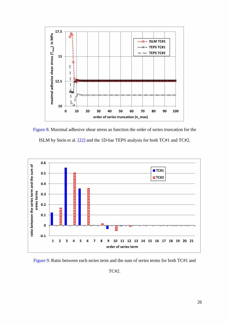
The maximal adhesive shear stress (Tmax) is provided in Figure 8 as function of the order of
series truncation (n_max) for both TC#1 and TC#2 as predicted by the ISLM and the TEPS
analysis. It is shown that Tmax tends to a finite value (12.56 MPa for TC#1 and 11.11 MPa for
TC#2) for an order of series truncations lower than n_max=20. For the case of n_max=100
with the TEPS analysis, the ratio between each series term Un with the sum of series terms –
which is equal to u(x=c) – is provided in Figure 9 for both TC#1 and TC#2, illustrating the
fast convergence of series. Moreover, the TEPS analysis provides a maximal adhesive shear
stress relatively different of 1.68E-4 % from the one provided by the ISLM (for TC#1).
26
Figure 8. Maximal adhesive shear stress as function the order of series truncation for the
ISLM by Stein et al. [22] and the 1D-bar TEPS analysis for both TC#1 and TC#2.
Figure 9. Ratio between each series term and the sum of series terms for both TC#1 and
TC#2.
10
12.5
15
17.5
0 10 20 30 40 50 60 70 80 90 100
max
imal
ad
he
sive
sh
ear
str
ess
(T
max
) in
MP
a
order of series truncation (n_max)
ISLM TC#1
TEPS TC#1
TEPS TC#2
-0.1
0
0.1
0.2
0.3
0.4
0.5
0.6
1 2 3 4 5 6 7 8 9 10 11 12 13 14 15 16 17 18 19 20 21
rati
o b
etw
ee
n t
he
se
rie
s te
rm a
nd
th
e s
um
of
sre
ies
term
s
order of series term
TC#1
TC#2

27
The relative difference in the maximal adhesive provided the 1D-bar ME analysis from the
one by 1D-bar TEPS analysis as function of the number of MEs for both TC#1 and TC#2 is
provided in Figure 10. It is shown that Tmax provided by the 1D-bar ME analysis tends to the
one provided by the TEPS analysis when the number of MEs is increased. For n_ME=1000,
the relative difference is 0.16% (0.22%) for TC#1 (TC#2). As a result, the TEPS resolution
scheme is less costly in terms of CPU time than the ME one, since convergence is obtained at
a lower size of the linear system to be inverted. This behavior is related to the meshing
strategy associated with the graduation of adhesive properties. It is thought that the number of
MEs could be reduced by adapting the length of each ME according to the current gradient of
adhesive properties for example. However, the mesh optimization is not the topic of this
paper. In Figure 11, the maximal adhesive shear stress provided by the 1D-bar and 1D-beam
analysis as function the order of the number of MEs for both TC#1 and TC#2 is provided. As
expected from Figure 10, it is shown that Tmax tends to a finite value.
Figure 10. Relative difference in % in the maximal adhesive provided the 1D-bar ME analysis
from the one by 1D-bar TEPS analysis as function of the number of MEs for both TC#1 and
TC#2.
0
10
20
30
40
50
60
0 200 400 600 800 1000
rela
tive
dif
fere
nce
in %
in T
max
number of ME (n_ME)
1D-bar ME TC#1
1D-bar ME TC#2
TC#2
TC#1

28
Figure 11. Maximal adhesive shear stress provided by the 1D-bar and 1D-beam analysis as
function the order of the number of MEs for both TC#1 and TC#2.
3.3. Elements of validation
The ME technique is a particular resolution scheme allowing for the system of ODEs coming
from simplifying hypotheses on which various models – such as Volkersen, Goland and
Reissner, Hart-Smith, Luo and Tong – are based. It was shown in that, for bonded joints with
constant adhesive properties under mechanical or thermal loads, the predictions from the
models using the ME resolution scheme provide the same results as those provided by the
related reference models [36-40]. In other words, the same hypotheses lead to the same
results. Moreover, it was shown that the predictions from the ME analysis are in close
agreements with those from FE models built on bar or beam element linked by peel and/or
shear springs, under mechanical and/or thermal loads, involving the update of adhesive
properties for each ME to take into account for nonlinear adhesive material behaviors [39-40].
These FE models were developed to be the most representative for the ME analysis in order to
validate the codes. As a result, the ME resolution scheme provide validated predictions
relevant to the simplifying hypotheses. Similarly, the TEPS resolution scheme allows for the
5
7.5
10
12.5
15
17.5
20
22.5
25
27.5
30
0 200 400 600 800 1000
max
imal
ad
he
sive
sh
ear
str
ess
(T
max
) in
M
Pa
number of ME (n_ME)
1D-bar ME TC#1 1D-bar ME TC#2
1D-beam TC#1 1D-beam TC#2
TC#1
TC#2
29
resolution of differential equations related to the simplifying equations. It was validated and
assessed in the case of FGA single-lap joints under mechanical load by Stein et al. [22].
In addition, the stress distributions at constant maximal and minimal adhesive properties are
then provided from the use of ME models in the following sections. An order of truncation
equal to 100 and a number of MEs equal to 500 is chosen in the following sections.
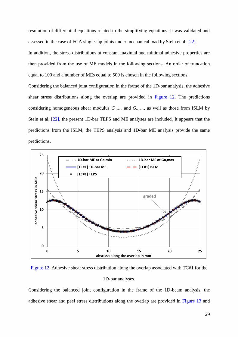
Considering the balanced joint configuration in the frame of the 1D-bar analysis, the adhesive
shear stress distributions along the overlap are provided in Figure 12. The predictions
considering homogeneous shear modulus Ga,min and Ga,max, as well as those from ISLM by
Stein et al. [22], the present 1D-bar TEPS and ME analyses are included. It appears that the
predictions from the ISLM, the TEPS analysis and 1D-bar ME analysis provide the same
predictions.
Figure 12. Adhesive shear stress distribution along the overlap associated with TC#1 for the
1D-bar analyses.
Considering the balanced joint configuration in the frame of the 1D-beam analysis, the
adhesive shear and peel stress distributions along the overlap are provided in Figure 13 and
0
5
10
15
20
25
0 5 10 15 20 25
adh
esi
ve s
he
ar s
tre
ss in
MP
a
abscissa along the overlap in mm
1D-bar ME at Ga,min 1D-bar ME at Ga,max
[TC#1] 1D-bar ME [TC#1] ISLM
[TC#1] TEPS
graded

30
Figure 14, respectively. The predictions considering homogeneous shear and peel modulus
(Ga,min ; Ea,min ) and (Ga,max ; Ea,max ), as well as those from GM by Stein et al. [22], the present
1D-beam ME analyses are included. As the simplifying hypotheses of the GM differ from
those used in the present 1D-beam analysis solved with the ME technique, the predictions
from the GM and 1D-beam ME analysis are not superimposed. Nevertheless, it appears that
the predictions are close each other and qualitatively similar. As expected, the predictions in
terms of adhesive shear stress by the 1D-bar analysis differ from those by the 1D-beam
analysis.
Figure 13. Adhesive shear stress distribution along the overlap associated with TC#1 for the
1D-beam analyses.
0
5
10
15
20
25
30
35
40
45
0 5 10 15 20 25
adh
esi
ve s
he
ar s
tre
ss in
MP
a
abscissa along the overlap in mm
1D-beam ME shear stress at Ea,min and Ga,min
1D-beam ME shear stress at Ea,max and Ga,max
[TC#1] 1D-beam ME shear stress
[TC#1] 1D-bar ME shear stress
[TC#1] GM shear stress
graded (GM)
graded (1D-beam ME)
graded 1D-bar

31
Figure 14. Adhesive peel stress distribution along the overlap associated with T C#1 for the
1D-beam analyses.
3.4. Test cases
3.4.1 1D-bar analyses
The adhesive shear stress distributions along the overlap are provided in Figure 15 and Figure
16 for the 1D-bar analyses for TC#2 and TC#3 (unbalanced joint configuration under
combined mechanical and thermal loads), respectively. The ISLM cannot then be applied. It is
shown that the predictions by the 1D-bar TEPS and ME analyses are superimposed. For each
case, the graduation of adhesive properties allows to reduce the peak stresses below those
obtained from the case at constant minimal shear modulus. However, the reduction is less
pronounced for the unbalanced cases (TC#2 and TC#3). For the TC#1, the reduction in
adhesive shear peak stress at x=c of the FGA joint is -21.7% from the bonded joints with a
constant shear modulus Ga,min, while it is -14.5% (-15.3%) for TC#2 (TC#3).
-20
-10
0
10
20
30
40
50
60
0 5 10 15 20 25
adh
esi
ve p
ee
l str
ess
in M
Pa
abscissa along the overlap in mm
1D-beam ME peel stress at Ea,min and Ga,min
1D-beam ME peel stress at Ea,max and Ga,max
[TC#1] 1D-beam ME peel stress
[TC#1] GM peel stress
graded (1D-beam ME)
graded (GM)

32
Figure 15. Adhesive shear stress distribution along the overlap associated with TC#2 for the
1D-bar analyses.
Figure 16. Adhesive shear stress distribution along the overlap associated with TC#3 for the
1D-bar analyses.
-25
-20
-15
-10
-5
0
5
10
15
20
25
0 5 10 15 20 25
adh
esi
ve s
he
ar s
tre
ss in
MP
a
abscissa along the overlap in mm
1D-bar ME at Ga,min 1D-bar ME at Ga,max
[TC#2] 1D-bar ME [TC#2] TEPS
graded
-10
0
10
20
30
40
50
60
70
80
0 5 10 15 20 25
adh
esi
ve s
he
ar s
tre
ss in
MP
a
abscissa along the overlap in mm
1D-bar ME at Ga,min 1D-bar ME at Ga,max
[TC#3] 1D-bar ME [TC#3] TEPS
graded
33
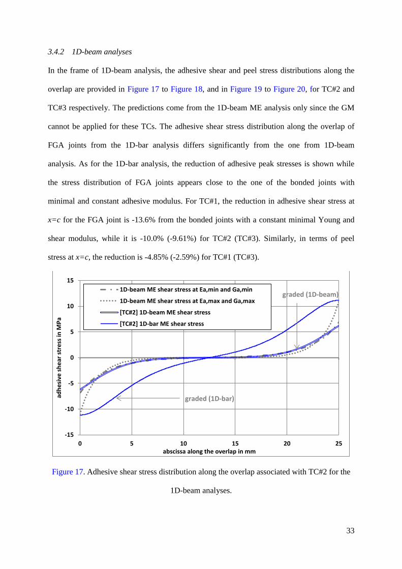
3.4.2 1D-beam analyses
In the frame of 1D-beam analysis, the adhesive shear and peel stress distributions along the
overlap are provided in Figure 17 to Figure 18, and in Figure 19 to Figure 20, for TC#2 and
TC#3 respectively. The predictions come from the 1D-beam ME analysis only since the GM
cannot be applied for these TCs. The adhesive shear stress distribution along the overlap of
FGA joints from the 1D-bar analysis differs significantly from the one from 1D-beam
analysis. As for the 1D-bar analysis, the reduction of adhesive peak stresses is shown while
the stress distribution of FGA joints appears close to the one of the bonded joints with
minimal and constant adhesive modulus. For TC#1, the reduction in adhesive shear stress at
x=c for the FGA joint is -13.6% from the bonded joints with a constant minimal Young and
shear modulus, while it is -10.0% (-9.61%) for TC#2 (TC#3). Similarly, in terms of peel
stress at x=c, the reduction is -4.85% (-2.59%) for TC#1 (TC#3).
Figure 17. Adhesive shear stress distribution along the overlap associated with TC#2 for the
1D-beam analyses.
-15
-10
-5
0
5
10
15
0 5 10 15 20 25
adh
esi
ve s
he
ar s
tre
ss in
MP
a
abscissa along the overlap in mm
1D-beam ME shear stress at Ea,min and Ga,min
1D-beam ME shear stress at Ea,max and Ga,max
[TC#2] 1D-beam ME shear stress
[TC#2] 1D-bar ME shear stress
graded (1D-beam)
graded (1D-bar)

34
Figure 18. Adhesive shear stress distribution along the overlap associated with TC#2 for the
1D-beam analyses.
Figure 19. Adhesive peel stress distribution along the overlap associated with TC#3 for the
1D-beam analyses.
-6
-5
-4
-3
-2
-1
0
1
2
0 5 10 15 20 25
adh
esi
ve p
ee
l str
ess
in M
Pa
abscissa along the overlap in mm
1D-beam ME peel stress at Ea,min and Ga,min
1D-beam ME peel stress at Ea,max and Ga,max
[TC#2] 1D-beam ME peel stress
graded
-10
0
10
20
30
40
50
60
70
80
0 5 10 15 20 25
adh
esi
ve s
he
ar s
tre
ss in
MP
a
abscissa along the overlap in mm
1D-beam ME shear stress at Ea,min and Ga,min
1D-beam ME shear stress at Ea,max and Ga,max
[TC#3] 1D-beam ME shear stress
[TC#3] 1D-bar ME shear stress
graded 1D- bar
graded 1D-beam

35
Figure 20. Adhesive peel stress distribution along the overlap associated with TC#3 for the
1D-beam analyses.
3.5. Reduction of adhesive peak stresses
This section aims at illustrating how the use of the 1D-beam ME analyses could help in the
design of adhesive graduation to reduce the adhesive peak stresses, for the unbalanced joint
configuration subjected to pure thermal load and combined mechanical and thermal loads in
particular. According to Hart-Smith [1,24], the adhesive peel stress could lead to an
anticipated failure of single-lap bonded joint, whereas the potential of shear deformation is
not reached. For the unbalanced joint configuration, under a pure thermal load, it is shown
that the level of adhesive peel stresses remain very low (see Figure 18), while the adhesive
shear stress are symmetrical in absolute value (see Figure 17). Under combined mechanical
and thermal loads, the level of adhesive peel stress is significantly higher due to the
introduction of the mechanical load inducing a bending moment at both overlap ends (see
Figure 20). Moreover, even if the adhesive peel stress distribution is asymmetrical due to the
-20
-10
0
10
20
30
40
50
0 5 10 15 20 25
adh
esi
ve p
ee
l str
ess
in M
Pa
abscissa along the overlap in mm
1D-beam ME peel stress at Ea,min and Ga,min
1D-beam ME peel stress at Ea,max and Ga,max
[TC#3] 1D-beam ME peel stress
graded

36
unbalance of the joint, the adhesive peel peaks stresses located at both overlap ends are
significant. As a result, for both previous load cases, a symmetrical adhesive graduation is
kept in order to try to reduce the adhesive peak stresses. It is assumed to follow a symmetrical
power law parametrized by p, with p=1,2,3,4, such as:
𝐸𝑎(𝑥) = 𝐸𝑎,𝑚𝑎𝑥(𝑥) − (𝐸𝑎,𝑚𝑎𝑥(𝑥) − 𝐸𝑎,𝑚𝑖𝑛(𝑥)) (𝑥
𝑐)2𝑝
(63)
𝐺𝑎(𝑥) = 𝐺𝑎,𝑚𝑎𝑥(𝑥) − (𝐺𝑎,𝑚𝑎𝑥(𝑥) − 𝐺𝑎,𝑚𝑖𝑛(𝑥)) (𝑥
𝑐)2𝑝
(64)
The increase of the parameter p allow for the enlargement of the overlap length at higher
modulus, while increasing the graduation slope at both overlap ends where the adhesive stress
gradients are higher. The shape of various graduations is illustrated in Figure 21.
Figure 21. Adhesive peel modulus along the overlap as a function of p.
Under a pure thermal load, the adhesive shear and peel stress distributions along the overlap
are provided in Figure 22 to Figure 23, respectively. It is shown that the level of adhesive peel
stresses remain low along the overlap. Relatively to the adhesive shear peak stresses with
p=1, a reduction of -5.13%, -4.56% and -1.78% is obtained with p=2, p=3 and p=4
respectively. Relatively to the adhesive stress at overlap end, where the level of adhesive peel
0
1000
2000
3000
4000
5000
6000
7000
0 5 10 15 20 25
adh
esi
ve p
ee
l mo
du
lus
in M
Pa
abscissa along te overlap in mm
p=1 p=2
p=3 p=4

37
stress is the highest, the reductions obtained become -5.22%, -8.42% and -10.6% with p=2,
p=3 and p=4 respectively. The choice of adhesive graduation law associated higher power
order allows then for a lag of the adhesive shear peak stress in direction of the center of the
overlap.
Figure 22. Adhesive shear stress distribution along the overlap for the unbalanced joint
configuration under a pure thermal load, for various adhesive graduations.
-7
-6
-5
-4
-3
-2
-1
0
1
2
3
4
5
6
7
0 5 10 15 20 25
adh
esi
ve s
he
ar s
tre
ss in
MP
a
abscissa along the overlap in mm
[graded with p=1] 1D-beam ME shear stress
[graded with p=2] 1D-beam ME shear stress
[graded with p=3] 1D-beam ME shear stress
[graded with p=4] 1D-beam ME shear stress
-3
-2
-1
0
1
0 5 10 15 20 25
adh
esi
ve p
ee
l str
ess
in M
Pa
abscissa along the overlap in mm
[graded with p=1] 1D-beam ME peel stress
[graded with p=2] 1D-beam ME peel stress
[graded with p=3] 1D-beam ME peel stress
[graded with p=4] 1D-beam ME peel stress

38
Figure 23. Adhesive peel stress distribution along the overlap for the unbalanced joint
configuration under a pure thermal load, for various adhesive graduations.
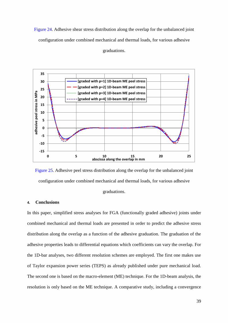
Under a combined mechanical and thermal load, the adhesive shear and peel stress
distributions along the overlap are provided in Figure 24 to Figure 25, respectively. As for the
pure thermal load case, the adhesive peak shear stresses are not located at both overlap ends
for p=2, p=3 and p=4. Relatively to the adhesive shear peak stresses with p=1 a reduction of
-4.80%, -5.39% and -3.18% is obtained with p=2, p=3 and p=4 respectively. Relatively to the
adhesive stress at overlap end, where the level of adhesive peel stress is the highest, the
reductions obtained become -4.80%, -7.76% and -9.77% with p=2, p=3 and p=4 respectively.
The adhesive peak peel stresses are located at both overlap ends; the maximal peak is located
at x=c. It is shown that with p=2, p=3 and p=4 respectively, both peaks at overlap ends are
reduced. Relatively to the adhesive peel peak stresses at x=c with p=1, a reduction of -2.87%,
-4.91% and -6.45% is obtained with p=2, p=3 and p=4 respectively
0
5
10
15
20
25
30
35
40
45
0 5 10 15 20 25
adh
esi
ve s
he
ar s
tre
ss in
MP
a
abscissa along the overlap in mm
[graded with p=1] 1D-beam ME shear stress
[graded with p=2] 1D-beam ME shear stress
[graded with p=3] 1D-beam ME shear stress
[graded with p=4] 1D-beam ME shear stress
39
Figure 24. Adhesive shear stress distribution along the overlap for the unbalanced joint
configuration under combined mechanical and thermal loads, for various adhesive
graduations.
Figure 25. Adhesive peel stress distribution along the overlap for the unbalanced joint
configuration under combined mechanical and thermal loads, for various adhesive
graduations.
4. Conclusions
In this paper, simplified stress analyses for FGA (functionally graded adhesive) joints under
combined mechanical and thermal loads are presented in order to predict the adhesive stress
distribution along the overlap as a function of the adhesive graduation. The graduation of the
adhesive properties leads to differential equations which coefficients can vary the overlap. For
the 1D-bar analyses, two different resolution schemes are employed. The first one makes use
of Taylor expansion power series (TEPS) as already published under pure mechanical load.
The second one is based on the macro-element (ME) technique. For the 1D-beam analysis, the
resolution is only based on the ME technique. A comparative study, including a convergence
-15
-10
-5
0
5
10
15
20
25
30
35
0 5 10 15 20 25
adh
esi
ve p
ee
l str
ess
in M
Pa
abscissa along the overlap in mm
[graded with p=1] 1D-beam ME peel stress
[graded with p=2] 1D-beam ME peel stress
[graded with p=3] 1D-beam ME peel stress
[graded with p=4] 1D-beam ME peel stress

40
study, is presented on balanced and unbalanced joint configuration under pure mechanical,
pure thermal and combined mechanical and thermal loads. The following conclusions could
then be made:
the present 1D-bar TEPS analysis restricted to a pure mechanical load provide the same
results as the ISLM by Stein et al [22];
the present 1D-bar TEPS and the 1D-bar ME analysis provide the same results;
the use of TEPS resolution scheme provides converged results at lower CPU cost than the
ME resolution scheme;
the graduation of the adhesive properties allows for the reduction of adhesive peak
stresses;
the present 1D-beam ME analysis restricted to a pure mechanical load provide similar
results as the GM by Stein et al [22];
the reduction of the adhesive shear peak stresses is found less pronounced when the 1D-
beam analysis is used instead of the 1D-bar analysis;
the reduction of the adhesive peak stresses in less pronounced for an unbalanced joint than
for a balance joint.
higher level of reduction can be obtained by modifying the graduation law.
A dedicated validation campaign based on FE modelling should be undertaken in order to
assess the relevance of the simplifying hypotheses and the performance of the resolution
scheme for the stress analysis of FGA joints. In particular, the free stress state at both overlap
ends cannot be captured with the simplifying hypotheses used. Besides, optimization
processes could be used to optimize the graduation of adhesive properties as function of the
adhesive stress distribution to minimize the adhesive peak stresses. Finally, in order to
increase the strength of FGA single-lap joints, an idea could be to graduate the properties of
both the adhesive and adherends. For example, the reduction of adhesive peel stresses at both

41
overlap ends could be obtain by tapering the adherend edge, while increasing the ratio
between the overlap length and the adherend thickness [1].
Acknowledgement
This work has not received any specific grant.
Appendix A
This appendix presents the mathematical description of the elementary stiffness matrix of the
BBa element. Equation Eq. (7) can be explicitly written such as a system of a coupled second
order ODE at constant coefficients:
{
𝑑2𝑢1
𝑑𝑋2+ 𝑘𝐼𝐼
1
𝑒1𝐸1(𝑢2 − 𝑢1) = 0
𝑑2𝑢2
𝑑𝑋2+ 𝑘𝐼𝐼
1
𝑒2𝐸2(𝑢2 − 𝑢1) = 0
(A-1)
This system is solved such as:
𝑢1(𝑋) =1
2(𝑐1 + 𝑐2𝑋 − 𝑐3(1 + 𝜒)𝑒
−𝜂𝑋 − 𝑐4(1 + 𝜒)𝑒𝜂𝑋) (A-2)
𝑢2(𝑋) =1
2(𝑐1 + 𝑐2𝑋 + 𝑐3(1 − 𝜒)𝑒
−𝜂𝑋 + 𝑐4(1 − 𝜒)𝑒𝜂𝑋) (A-3)
with:
𝜒 =𝜓2
𝜂2 (A-4)
𝜓2 =𝐺
𝑒(1
𝑒1𝐸1−
1
𝑒2𝐸2) (A-5)
𝜂2 =𝐺
𝑒(1
𝑒1𝐸1+
1
𝑒2𝐸2) (A-6)
where c1, c2, c3 and c4 are integration constants. The boundary conditions at both extremities of the
BBa element, in terms of displacements, lead to the expressions for the integration constants as
functions of nodal displacements ui, uj, uk and ul (see Figure 4):
𝑐1 = (1 − 𝜒)𝑢𝑖 + (1 + 𝜒)𝑢𝑗 (A-7)

42
𝑐2 = −(1−𝜒)
Δ𝑢𝑖 −
(1+𝜒)
Δ𝑢𝑗 +
(1−𝜒)
Δ𝑢𝑘 +
(1+𝜒)
Δ𝑢𝑙 (A-8)
𝑐3 = −𝑒𝜂Δ
2 sinh𝜂Δ𝑢𝑖 +
𝑒𝜂Δ
2 sinh𝜂Δ𝑢𝑗 +
1
2 sinh𝜂Δ𝑢𝑘 −
1
2 sinh𝜂Δ𝑢𝑙 (A-9)
𝑐4 =𝑒−𝜂Δ
2 sinh𝜂Δ𝑢𝑖 −
𝑒𝜂−Δ
2 sinh𝜂Δ𝑢𝑗 −
1
2sinh𝜂Δ𝑢𝑘 +
1
2sinh𝜂Δ𝑢𝑙 (A-10)
It can then be written under this shape:
𝐶 = (
𝑐1𝑐2𝑐3𝑐4
) = 𝑀𝑒−1𝑈𝑒 (A-11)
With:
𝑀𝑒−1 =
(
(1 − 𝜒) (1 + 𝜒) 0 0
−(1−𝜒)
Δ−(1+𝜒)
Δ
(1−𝜒)
Δ
(1+𝜒)
Δ
−𝑒𝜂Δ
2sinh𝜂Δ
𝑒𝜂Δ
2 sinh𝜂Δ
1
2 sinh𝜂Δ−
1
2 sinh𝜂Δ
𝑒−𝜂Δ
2 sinh𝜂Δ−
𝑒𝜂−Δ
2 sinh𝜂Δ−
1
2 sinh𝜂Δ
1
2sinh𝜂Δ )
(A-12)
The normal forces are then computed from Eq. (2), Eq. (A-2) and Eq. (A-3):
𝑁1(𝑋) =1
2(𝑐2 + 𝑐3𝜂(1 + 𝜒)𝑒
−𝜂𝑋 − 𝜂𝑐4(1 + 𝜒)𝑒𝜂𝑋)𝐴1 − 𝐴1𝛼1Δ𝑇 (A-13)
𝑁2(𝑋) =1
2(𝑐2 − 𝑐3𝜂(1 − 𝜒)𝑒
−𝜂𝑋 + 𝜂𝑐4(1 − 𝜒)𝑒𝜂𝑋)𝐴2 − 𝐴2𝛼2Δ𝑇 (A-14)
The nodal normal forces are then deduced as function of the integration constants:
𝐹𝑒 + (
−𝐴1𝛼1−𝐴2𝛼2𝐴1𝛼1𝐴2𝛼2
)Δ𝑇 = 𝑁𝑒𝐶 (A-15)
with:
𝑁𝑒 =1
2
(
0 −𝐴1 −𝜂(1 + 𝜒)𝐴1 𝜂(1 + 𝜒)𝐴10 −𝐴2 𝜂(1 − 𝜒)𝐴2 −𝜂(1 − 𝜒)𝐴20 𝐴1 𝜂(1 + 𝜒)𝑒−𝜂Δ𝐴1 −𝜂(1 + 𝜒)𝑒𝜂Δ𝐴10 𝐴2 −𝜂(1 − 𝜒)𝑒−𝜂Δ𝐴2 𝜂(1 − 𝜒)𝑒𝜂Δ𝐴2 )
(A-16)
In equation Eq. (A-15) the equivalent nodal force vector to the thermal load is appearing:

43
𝐹𝑡ℎ = (
−𝐴1𝛼1−𝐴2𝛼2𝐴1𝛼1𝐴2𝛼2
)Δ𝑇 (A-17)
From Eq. (A-11) and Eq. (A-15), it comes:
𝐹𝑒 + 𝐹𝑡ℎ = 𝑁𝑒𝑀𝑒−1𝑈𝑒 (A-18)
The elementary stiffness matrix is finally computed from the matrix Me and Ne:
𝐾𝐵𝐵𝑎 = 𝑁𝑒𝑀𝑒−1 =
1
1+𝜒𝐴
𝐴2
Δ
(
𝜂Δ
tanh𝜂Δ+
1
𝜒𝐴1 −
𝜂Δ
tanh𝜂Δ−
𝜂Δ
sinh𝜂Δ−
1
𝜒𝐴
𝜂Δ
sinh𝜂Δ− 1
1 −𝜂Δ
tanh𝜂Δ
𝜂Δ
tanh𝜂Δ+ 𝜒𝐴
𝜂Δ
sinh𝜂Δ− 1 −
𝜂Δ
sinh𝜂Δ− 𝜒𝐴
−𝜂Δ
sinh𝜂Δ−
1
𝜒𝐴
𝜂Δ
sinh𝜂Δ− 1
𝜂Δ
tanh𝜂Δ+
1
𝜒𝐴1 −
𝜂Δ
tanh𝜂Δ
𝜂Δ
sinh𝜂Δ− 1 −
𝜂Δ
sinh𝜂Δ− 𝜒𝐴 1 −
𝜂Δ
tanh𝜂Δ
𝜂Δ
tanh𝜂Δ+ 𝜒𝐴 )
(A-19)
The elementary stiffness matrix of the bar element, simulating the adherend j outside the
overlap is:
𝐾𝑏𝑎𝑟,𝑗 = 𝐴𝑗 (1 −1−1 1
) , 𝑗 = 1,2 (A-20)
Appendix B
This appendix provides the derivation of the constitutive equations of laminated beams used
in the 1D-beam analysis, in the (X,Yi,Z) reference local axis of the adherend, the height origin
of which is taken on the neutral axis. The normal force and the bending moment are written
such as:
𝑁𝑖(𝑋) = ∫ 𝜎𝑖𝑏𝑑𝑌𝑖+ℎ𝑖−ℎ𝑖
= 𝑏∑ ∫ 𝜎𝑖𝑝𝑖𝑑𝑌𝑖
ℎ𝑝𝑖ℎ𝑝𝑖−1
𝑛𝑖𝑝𝑖=1
, 𝑖 = 1,2 (B-1)
𝑀𝑖(𝑋) = ∫ −𝑌𝑖𝜎𝑖𝑏𝑑𝑌𝑖+ℎ𝑖−ℎ𝑖
= −𝑏∑ ∫ 𝜎𝑖𝑝𝑖𝑌𝑖𝑑𝑌𝑖
ℎ𝑝𝑖ℎ𝑝𝑖−1
𝑛𝑖𝑝𝑖=1
, 𝑖 = 1,2 (B-2)
where, in the adherend i ni is the number of layers and hpi is the final height of the pith
layer.
Moreover, the orthotopic behavior provides
𝜎𝑖𝑝𝑖 = 𝑄𝑖
𝑝𝑖(𝜀𝑖𝑝𝑖 − 𝛼𝑖
𝑝𝑖Δ𝑇), 𝑖 = 1,2 (B-3)

44
where, in the adherend I, 𝑄𝑖𝑝𝑖 is the matrix of reduced stiffness in the pi
th layer.
As a result, the normal force and the bending moment are given by:
𝑁𝑖(𝑋) = 𝑏∑ ∫ 𝑄𝑖𝑝𝑖(𝜀𝑖
𝑝𝑖 − 𝛼𝑖𝑝𝑖Δ𝑇)𝑑𝑌𝑖
ℎ𝑝𝑖ℎ𝑝𝑖−1
𝑛𝑖𝑝𝑖=1
, 𝑖 = 1,2 (B-4)
𝑀𝑖(𝑋) = −𝑏∑ ∫ 𝑄𝑖𝑝𝑖(𝜀𝑖
𝑝𝑖 − 𝛼𝑖𝑝𝑖Δ𝑇)𝑌𝑖𝑑𝑌𝑖
ℎ𝑝𝑖ℎ𝑝𝑖−1
𝑛𝑖𝑝𝑖=1
𝑖 = 1,2 (B-5)
which finally leads to:
𝑁𝑖(𝑥) =
∑ 𝑄𝑖𝑝𝑖 [∫ 𝑑𝑦𝑖
ℎ𝑝𝑖ℎ𝑝𝑖−1
]𝑛𝑖𝑝𝑖=1
𝑑𝑢𝑖
𝑑𝑥− 𝑏∑ 𝑄𝑖
𝑝𝑖 [∫ 𝑦𝑖𝑑𝑦𝑖ℎ𝑝𝑖ℎ𝑝𝑖−1
]𝑛𝑖𝑝𝑖=1
𝑑𝜃𝑖
𝑑𝑥− 𝑏∑ 𝑄𝑖
𝑝𝑖𝛼𝑖𝑝𝑖 [∫ 𝑑𝑦𝑖
ℎ𝑝𝑖ℎ𝑝𝑖−1
]𝑛𝑖𝑝𝑖=1
Δ𝑇
(B-6)
𝑀𝑖(𝑥) =
𝑏∑ 𝑄𝑖𝑝𝑖 [∫ 𝑦𝑖𝑑𝑦𝑖
ℎ𝑝𝑖ℎ𝑝𝑖−1
]𝑛𝑖𝑝𝑖=1
𝑑𝑢𝑖
𝑑𝑥+ 𝑏∑ 𝑄𝑖
𝑝𝑖 [∫ 𝑦𝑖2𝑑𝑦𝑖
ℎ𝑝𝑖ℎ𝑝𝑖−1
]𝑛𝑖𝑝𝑖=1
𝑑𝜃𝑖
𝑑𝑥+
∑ 𝑄𝑖𝑝𝑖𝛼𝑖
𝑝𝑖 [∫ 𝑦𝑖𝑑𝑦𝑖ℎ𝑝𝑖ℎ𝑝𝑖−1
] Δ𝑇𝑛𝑖𝑝𝑖=1
(B-7)
The parameters involving in the constitutive equations Eq. (31) to Eq. (33) are thus defined
such as for i=1,2
𝐴𝑖 = 𝑏∑ 𝑄𝑖𝑝𝑖(ℎ𝑝𝑖 − ℎ𝑝𝑖−1)
𝑛𝑖𝑝𝑖=1
(B-8)
𝐵𝑖 =𝑏
2∑ 𝑄𝑖
𝑝𝑖(ℎ𝑝𝑖2 − ℎ𝑝𝑖−1
2)𝑛𝑖𝑝𝑖=1
(B-9)
𝐷𝑖 =𝑏
3∑ 𝑄𝑖
𝑝𝑖(ℎ𝑝𝑖3 − ℎ𝑝𝑖−1
3)𝑛𝑖𝑝𝑖=1
(B-10)
𝑁𝑖�̅� = 𝑏∑ 𝑄𝑖
𝑝𝑖𝛼𝑖𝑝𝑖(ℎ𝑝𝑖 − ℎ𝑝𝑖−1)
𝑛𝑖𝑝𝑖=1
Δ𝑇 (B-11)
𝑀𝑖�̅� =
𝑏
2∑ 𝑄𝑖
𝑝𝑖𝛼𝑖𝑝𝑖(ℎ𝑝𝑖
2 − ℎ𝑝𝑖−12)
𝑛𝑖𝑝𝑖=1
Δ𝑇 (B-12)
Appendix C

45
This appendix provides a brief description of the formulation of the beam element used in the
1D-beam analysis. Under the approximation of small bending angle, the local equilibrium
equations of adherend i=1,2 outside the overlap are given by:
𝑑𝑁𝑖
𝑑𝑋= 0 (C-1)
𝑑𝑉𝑖
𝑑𝑋= 0 (C-2)
𝑑𝑀𝑖
𝑑𝑋+ 𝑉𝑖 − 𝑁𝑖𝜃𝑖 = 0 (C-3)
It corresponds to those obtained along the overlap when the adhesive stresses vanish. But, the
normal force is equal to F at any X. The system of six first order linear ODEs to be solved is
then found under the following shape:
𝑑𝑢𝑖
𝑑𝑋=𝐷𝑖
Δ𝑖𝑁1 +
𝐵𝑖
Δ𝑖𝑀𝑖 (C-4)
𝑑𝑣𝑖
𝑑𝑋= 𝜃𝑖 (C-5)
𝑑𝜃𝑖
𝑑𝑋=𝐵𝑖
Δ𝑖𝑁𝑖 +
𝐴𝑖
Δ𝑖𝑀𝑖 (C-6)
𝑑𝑁𝑖
𝑑𝑋= 0 (C-7)
𝑑𝑉𝑖
𝑑𝑋= 0 (C-8)
𝑑𝑀𝑖
𝑑𝑋= −𝑉𝑖 + 𝐹𝜃𝑖 (C-9)
The resolution is performed using the exponential matrix as described in section 2.2.3.
Appendix D
In [39-40], a path to take into account for a linear variation of the shear stress in the adherend
thickness following [28] in the formulation of MEs is described and reminded here. In the 1D-
bar analysis, it is sufficient to modify the adhesive shear relative stiffness such as:
𝑘𝐼𝐼 =1
1+𝛽
𝐺𝑎
𝑒𝑎 (D-1)
with:

46
𝛽 =1
3
𝐺𝑎
𝑒𝑎(𝑒1
𝐺1+𝑒2
𝐺2) (D-2)
where G1 (G2) is the shear modulus of the adherend 1 (2).
In the 1D-beam analysis, the constitutive equations of adherends to consider are:
𝑁𝑖 = 𝐴𝑖𝑑𝑢𝑖
𝑑𝑥− 𝐵𝑖
𝑑𝜃𝑖
𝑑𝑥− 𝐶𝑖
𝑑𝑇
𝑑𝑥− 𝑁𝑖
Δ𝑇 (D-3)
𝑀𝑖 = −𝐵𝑖𝑑𝑢𝑖
𝑑𝑥+𝐷𝑖
𝑑𝜃𝑖
𝑑𝑥+ 𝐶′𝑖
𝑑𝑇
𝑑𝑥+𝑀𝑖
Δ𝑇 (D-4)
𝜃𝑖 =𝑑𝑣𝑖
𝑑𝑥 (D-5)
where, for i=1,2:
𝐶𝑖 =𝑒𝑖𝐵𝑖+(−1)
𝑖𝐷𝑖
2𝑒𝑖𝐺𝑖=1
2(𝐵𝑖
𝐺𝑖+ (−1)𝑖
𝐷𝑖
2ℎ𝑖𝐺𝑖) (D-6)
𝐶′𝑖 =𝑒𝑖𝐷𝑖+(−1)
𝑖𝐹𝑖
2𝑒𝑖𝐺𝑖=1
2(𝐷𝑖
𝐺𝑖+ (−1)𝑖
𝐹𝑖
2ℎ𝑖𝐺𝑖) (D-7)
𝐹𝑖 =𝑏
4∑ 𝑄𝑖
𝑝𝑖(ℎ𝑝𝑖4 − ℎ𝑝𝑖−1
4)𝑛𝑖𝑝𝑖=1
(D-8)
Beside, to replace the Euler-Bernoulli beam model by the beam model, it is sufficient to
replace the normality equation:
𝑑𝑣𝑖
𝑑𝑋= 𝜃𝑖 (D-9)
by:
𝑉𝑖 = 𝐻𝑖 (𝑑𝑣𝑖
𝑑𝑥− 𝜃𝑖) (D-10)
where Hi is the shear stiffness taken into account the shear correction factor.
References
1. Hart-Smith, LJ, 1982. Design methodology for bonded-bolted composite joints. Technical
Report, AFWAL-TR-81-3154, Douglas Aircraft Company, Long Beach, California.
2. Kelly, G, 2006. Quasi-static strength and fatigue life of hybrid (bonded/bolted) composite
single-lap joints. Compos. Struct., 72, 119-129.

47
3. da Silva, LFM, Öschner, A, Adams, RD (Editors), 2018. Handbook of Adhesion
Technology (2 volumes), 2nd
edition Springer, Heidelberg, Germany.
4. ASTM D5656-95. Standard Test Method for Thick-Adherend Metal Lap-Shear Joints for
the Stress-strain Behavior of adhesives by Tension Loading. ASTM 1995.
5. Cognard, JY, Créac’hcadec, R, Sohier, L, Leguillon, D, 2010. Influence of adhesive
thickness on the behaviour of bonded assemblies under shear loadings using a modified TAST
fixture. Int. J. Adhes. Adhes., 30, 257-266.
6. Hart-Smith, LJ, 1973. Adhesive-bonded scarf and stepped-lap joints. Technical Report,
NASA, CR112237, Douglas Aircraft Company, Long Beach, California.
7. Oterkus, E., Barut, A., Madenci, E., Smeltzer, S.S., Ambur, D.R., 2004. Nonlinear analysis
of bonded composite joints, 45th AIAA/ASME/ASCE/AHS/ASC Structures, Structural
Dynamics, and Materials Conference, 19-22 April 2004, Palm Springs, California.
8. Zhao, X, Adams, RD, da Silva, LFM, 2011a. Single lap joints with rounded adherend
corners: Stress and strain analysis. J. Adhes. Sci. Technol., 25, 819-836.
9. Zhao, X, Adams, RD, da Silva, LFM, 2011b. Single lap joints with rounded adherend
corners: Experimental results and strength prediction, J. Adhes. Sci. Technol., 25, 837-856.
10. Raphael, C, 1966. Variable-adhesive bonded joints. In: Proceedings of the Applied
Polymer Symposium, 3, 99-108.
11. da Silva, LFM, Lopes, MJCQ, 2009. Joint strength optimization by the mixed-adhesive
technique. . Int. J. Adhes. Adhes., 29(5), 509-514.
12. Breto, R, Chiminelli, A, Duvivier, E, Lizaranzu, M, Jiménez, MA, 2015. Finite Element
Analysis of Functionally Graded Bond-Lines for Metal/Composite Joints. J. Adhesion, 91,
920-936.
13. Machado, J, Marques, E, da Silva, LFM, 2018. Influence of low and high temperature on
mixed adhesive joints under quasi-static and impact conditions. Compos. Struct., 194, 68-79.

48
14. Durodola, JF, 2017. Functionally graded adhesive joints – A review and prospects. Int. J.
Adhes. Adhes., 76, 83-89.
15. Kawasaki, S, Nakajima, G, Haraga, K, Sato, C, 2016. Functionally Graded Adhesive
Joints Bonded by Honeymoon Adhesion Using Two Types of Second Generation Acrylic
Adhesives of Two Components. J. Adhesion, 92(7-9), 517-534.
16. van Ingen, JW, Vlot, A, 1993. Stress analysis of adhesively bonded single lap joints.
Report LR-740, Delft University of Technology. The Netherlands.
17. Tsaï, MY, Morton, J, 1994. An evaluation of analytical and numerical solutions to the
single-lap joint. Int. J. Solids Struct., 31, 2537-2563.
18. da Silva, LFM, das Neves, PJC, Adams, RD, Spelt, JK, 2009. Analytical models of
adhesively bonded joints-Part I: Literature survey. Int. J. Adhes. Adhes., 29, 319-330.
19. Carbas, RJC, da Silva, LFM, Madureira, ML, Critchlow, GW, 2014. Modelling of
functionally graded adhesive joints. J. Adhesion, 90(8), 698-716.
20. Volkersen, O, 1938. Die Nietkraftverteilung in Zugbeanspruchten Nietverbindungen mit
konstanten Laschenquerschnitten, Luftfahrforschung. 15(24), 41-47.
21. Stein, N, Weißgraeber, P, Becker, W, 2016. Stress solution for functionally graded
adhesive joints. Int. J. Solids Struct., 97-98, 300-311.
22. Stein, N, Felger, J, Becker, W, 2017. Analytical models for functionally graded adhesive
joints: A comparative study, Int. J. Adhes. Adhes., 76, 70-82.
23. Goland, M, Reissner, E, 1944. The stresses in cemented joints, J. Appl. Mech., 11, A17-
A27.
24. Hart-Smith, LJ, 1973. Adhesive bonded single lap joints. NASA Technical Report, CR-
112236, Douglas Aircraft Company, Long Beach, California.
25. Williams, JH, 1975. Stresses in adhesive between dissimilar adherends. J. Adhesion, 7,
97-107.
49
26. Bigwood, DA, Crocombe AD, 1989. Elastic analysis and engineering design formulae for
bonded joints. Int. J. Adhes. Adhes., 9(4), 229-242.
27. Oplinger, DW, 1991. A Layered Beam Theory for Single-Lap Joints, Technical Report,
US AMTL, MTL91-23.
28. Tsaï, MY, Oplinger, DW, Morton, J., 1998. Improved Theoretical Solutions for Adhesive
Lap Joints Int. J. Solids Struct., 35(12), 1163-1185.
29. Högberg, JL, 2004. Mechanical behavior of single-layer adhesive joints – An Integrated
approach. Licensing Graduate Thesis, Department of Applied Mechanics, Chalmers
University of Technology, Sweden.
30. Nemes, O, Lachaud, F, 2009. Modeling of cylindrical adhesively bonded joints, J. Adhes.
Sci. Technol., 23(10-11), 1383-1393.
31. Luo, Q, Tong, L, 2007. Fully-coupled nonlinear analysis of single lap adhesive joints. Int.
J. Solids Struct., 44, 2349-2370.
32. Weißgraeber, P, Stein, N, Becker, W, 2014. A general sandwich-type model for adhesive
joints with composite adherends. Int. J. Adhes. Adhes., 55, 56–63.
33. Talmon de l’Armée, A, Stein, N, Becker, W, 2016. Bending moment calculation for single
lap joints. Int. J. Solids Struct., 66, 41–52.
34. Stapleton, SE, Weimer, J, Spengler, J, 2017. Design of functionally graded joints using a
polyurethane-based adhesive with varying amounts of acrylate, Int. J. Adhes. Adhes., 76, 38-
46.
35. Stapleton, SE, 2012. The analysis of adhesively bonded advanced composite joints using
joint finite elements. PhD thesis, University of Michigan. Michigan.
36. Paroissien, E, 2006. Contribution aux Assemblages Hybrides (Boulonnés/Collés) –
Application aux Jonctions Aéronautiques. PhD Dissertation (in French), Université de
Toulouse III.
50
37. Paroissien, E, Sartor, M, Huet, J, 2007. Hybrid (bolted/bonded) joints applied to
aeronautic parts: Analytical one-dimensional models of a single-lap joint. In: Advanced in
Integrated Design and Manufacturing in Mechanical Engineering II. S Tichkiewitch, M
Tollenaere, and P Ray (Eds.), 95-110, Springer, Dordrecht, The Netherlands.
38. Paroissien, E, Sartor, M, Huet, J, Lachaud, F, 2007. Analytical two-dimensional model of
a hybrid (bolted/bonded) single-lap joint, J. Aircraft, 44, 573-582.
39. Paroissien, E, Lachaud, F, Jacobs T, 2013. A simplified stress analysis of bonded joints
using macro-elements. In: Advances in Modeling and Design of Adhesively Bonded Systems,
Kumar S. and Mittal K.L. (Eds), 93-146, Wiley-Scrivener, Beverly, Massachusetts.
40. Paroissien, E, Gaubert, F, Da Veiga, A, Lachaud, F, 2013. Elasto-Plastic Analysis of
Bonded Joints with Macro-Elements. J. Adhes. Sci. Technol., 27(13), 1464-1498.
41. Lélias, G, Paroissien, E, Lachaud, F, Morlier, J, Schwartz, S, Gavoille, C, 2015. An
extended semi-analytical formulation for fast and reliable mode I/II stress analysis of
adhesively bonded joints. Int. J. Solids Struct., 62, 18-38.
42. Lélias, G, 2016. Mechanical behavior of adhesively bonded joints: Modeling, simulation
and experimental characterization. PhD Thesis, University of Toulouse 3, Toulouse, France.
43. Paroissien, E, Lachaud, F, Da Veiga, A, Barrière, P, 2017. Simplified Stress Analysis of
Hybrid (Bolted/Bonded) Joints. Int. J. Adhes. Adhes., 77, 183-197.
44. Hart-Smith, LJ, 1973c. Adhesive-Bonded Double-Lap Joints. NASA Technical Report,
CR112235, Douglas Aircraft Company, Long Beach, California.
45. Zeyfang, R, 1971. Stresses and strains in a plate bonded to a substrate: Semiconductor
devices. Solid State Electron., 14, 1035-1039.
46. Chen, WT, Nelson, CW, 1979. Thermal stresses in Bonded Joints. IBM J. R&D, 23(2),
179-188.
47. Suhir, E, 1986. Stresses in bi-material thermostat. J. Appl. Mech., 53, 657-660.

51
48. Marques, EAS, da Silva, LFM, Banea, MD, Carbas, R, 2015. Adhesive joints for low and
high temperature use: An overview. J. Adhesion, 91, 556–585.
Top Related