


Languages
Pages
Legal


1
Analysis of Factors AffectingThe Winning Percentage of One Day International (ODI) Cricket Matches
MATH 240PROFESSOR LANCE ROBINS
SUMMER 2015
By
REDDY BHARGAVI KAPUGANTI (0579749)
SAI RAJU JAMPANA (0576385)
VENU GOPAL VEGI (0578423)
POORVA PATIL (578850)

2
Table on Contents
Introduction – (Brief Background & Assumptions)………………………….3
Problem Statement……………………………………………………………..4
Test Design/Approach………………………………………………………….4
Results of Data Analysis/Testing………………………………………………5
Conclusion…………………….………………………………………………...9
References………………………………………………………………….......10
Appendix - (Data Formatted from Excel)……………………………………11
Descriptive Stats………………………………………………………...11
Linear Regression & Scatter Plots.........................................................13
Multiple Regression……………………………………………….……21

3
Introduction
In this paper we endeavor to dissect the elements influencing the winning percentage in
One Day International (ODI) Cricket Matches considering the investigation of most recent 10
years. Separate relapse trials are distinguished for the examination of ODI among different
countries. This examination ought to give knowledge on exactly how vital every variable is, for
the execution of the teams in winning. Our group decided to break down the variables inside of
the one-day international cricket matches, on account of our interest in Cricket. We as students
of India had the delight of seeing the Indians win the latest series. Each of the four of us is from
India, so when India won match this year it was energizing, as everybody bolstered and
commended their win. In spite of the fact that we were not ready to exclusively concentrate on
the Indian cricket group as the information would be excessively restricted, we chose, making it
impossible to extend our center to the whole ODI. In this way we chose to check whether we
could figure out what variables inside ODI information would prompt a higher winning rate.
Our group gathered information from ESPN.com. The information gathered was of the 21
teams in one day global amid the normal season traversing from 10 years. We expressed the
needy variable as the winning rate, computed the winning percentage by dividing total matches
won by the total matches played. In addition we considered other important variables as Average
(Batting), Average (Bowling), Strike Rate (Bowling) and Highest Scores.
The independent variables that are considered are Average (Batting), Average (Bowling),
Strike Rate (Bowling) and Highest Scores. However, the dependent variable is Winning
Percentage. To score is to hit runs and expecting a team can score more runs, we must accept that
their batting attitudes are nice. In addition to this in bowling, the team is concerned on taking
wickets and maintaining proper average or run rate. Thus, we as a team have predicted that of all
the variables tested, the batting & bowling stats will yield the strongest linear relationship to the
winning percentage.
The free variables that group under bowling details are no ball, wide ball, run rate and
wickets taken. No ball is the point at which a bowler tosses over the height of the batsman or
bowling off the crease. Wide ball is the point at which the bowler bowls a ball which is too away

4
from the wide crease. Run-rate is the runs given in a bowling over. Finally, wickets taken are
number of dismissals either by stump-outs; run-outs, lbw’s or catches. Bowling strike rate is
defined for a bowler as the average number of balls bowled per wicket taken. All these variables
are considered for the total average of bowling and strike rate.
Lastly, the free variables that group under batting details are runs and strike rate. Batting
strike rate is defined for a batsman as the average number of runs scored per 100 balls faced. The
higher the strike rate, the more effective a batsman is at scoring quickly. Runs are scored by a
batsman, and the aggregate of the scores of a team's batsmen (plus any extras) constitutes the
team's score. All these variables are considered for the total average of batting and strike rate.
Problem Statement
Our team chose to analyze the relationship of different details and the general winning
rate to better comprehend what constitutes a "winning group". In spite of the fact that we might
never be sure to what precisely constitutes a triumphant group, we might want to think our
outcomes will reveal some insight into what details to search for, in a team who has a higher
winning rate. We decided to break down the accompanying independent variables to see which
had the most influence on the winning rate: Average (Batting), Average (Bowling), Strike Rate
(Bowling) and Highest Score.
Test Design/Approach
This research paper is based on the data collected from the ESPN ODI official website
for the games played by 21 ODI teams within the last 10 years. The Excel data found in our
appendix contains data such as winning percentage, highest score, strike rate, average batting and
bowling.
Based on the acquired data, the first step was to perform the descriptive statistics. This
would give us a summary of the observations by analyzing the measures of central tendency
(mean, median, and mode), variation (rage, interquartile range, variance, standard deviation,
coefficient of variation), shape (skewness) etc.

5
The second step was performing a linear regression analysis with each independent
variable in relationship to our dependent variable. The dependent variable chosen is Winning
percentage and the independent variables chosen are Average (Batting), Average (Bowling),
Strike Rate (Bowling) and Highest Score. This was performed to detect the strength of a
relationship between the two respected variables and by analyzing the scatter plot, measures of
variation, standard errors, intercept etc.
Next, we performed a numerous relapse examination, with the greater part of our
independent variables in relationship to our dependent variable (winning rate). This examination
spoke to the error between the real and anticipated worth served to analyze completely the
accompanying suppositions: linearity, autonomy and ordinariness, square with fluctuation, the
Durbin-Watson insights, leftover plot, t detail, p esteem and so forth. These outcomes would
permit us to investigate the relationship of one needy variable and more autonomous variables by
looking at the coefficient of numerous determinations (r2), balanced sr2 and the general F test.
The noteworthiness of the variables was dictated by the p-estimation of 0.05 or less:
If the p-worth is more noteworthy than or equivalent to α, don't dismiss the invalid
speculation;
If the p-worth is not as much as, reject the invalid speculation. As a final step, the
variable model was chosen as the most appropriate for our case and several tests were
conducted to check its assumptions including t-test, hypothesis test, regression analysis, p
value etc.
Results
We ran a multiple regression analysis as well as a simple linear regression on the data. The
simple linear regression results can be found in our Appendix. The multiple regression models
came out as significant. The variables batting average and bowling average affected the winning
percentage. We also noticed that both batting average and bowling average have an impact on
the winning percentage along with team performance. Therefore, for every change in the value of
batting average or blowing average will have an effect on winning percentage.

6
Coefficients P-valueIntercept 0.1468 0.0344Ave(Batting) 0.0095 0.0000AVE(BOWLING) 0.0113 0.0000SR(BOWLING) -0.0057 0.0659HS 0.0003 0.0229
There was no need to re-run the multiple regression analysis again as the first model was
significant in itself, returning the p-values which are considerable for every relationship. The
multiple regressions were run on 95% confidence interval. The model has r square value
of .9646 and adjusted r square value of .9558, which represents a good number. The r square
number did not improve even if the least affecting independent variable was removed indicating
this to be the best option.
The effect of bowling average is interdependent on batting average score as well, since
they both contribute to winning percentage. Sure, teams might have a positive impact on their
home countries, but the absence of better bowling might change the game. Same as the batting
pitch has an impact on bowling, the blowing pitch would have impact the batting score. In this
case both terms have an impact on total score and winning percentage.
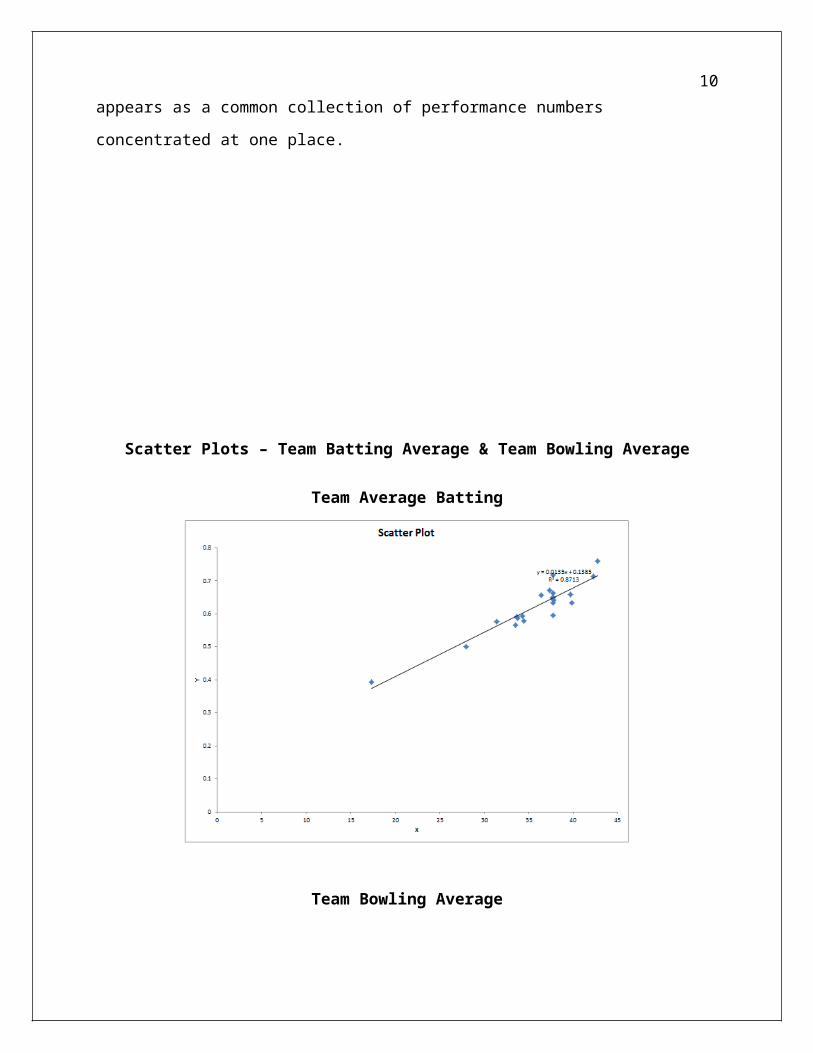
We have included the scatter plots for both of them below. The plots also go hand in hand
with this information and it is quite clear that the data for strike rate (bowling) and highest score
are quite scattered whereas average batting and bowling appears as a common collection of
performance numbers concentrated at one place.

7
Scatter Plots – Team Batting Average & Team Bowling Average
Team Average Batting
Team Bowling Average

8
The Multiple Regression Output
Regression StatisticsMultiple R 0.9821R Square 0.9646Adjusted R Square 0.9558Standard Error 0.0165Observations 21
ANOVA
df SS MS FSignificanc
e F
Regression 4 0.11850.029
6109.034
2 0.0000
Residual 16 0.00430.000
3Total 20 0.1228
Coefficients
Standard Error t Stat P-value Lower 95%
Upper 95%
Intercept 0.1468 0.06352.312
3 0.0344 0.0122 0.2814
Ave(Batting) 0.0095 0.00118.834
2 0.0000 0.0072 0.0118
AVE(BOWLING) 0.0113 0.00205.574
9 0.0000 0.0070 0.0156
SR(BOWLING) -0.0057 0.0029
-1.974
2 0.0659 -0.0118 0.0004
HS 0.0003 0.00012.516
2 0.0229 0.0000 0.0005

9
Conclusion
The above illustration indicates that the coefficients are depicting correct relationships
with the dependent variable. For instance, the variables like Average Batting and Average
Bowling have positive impact on the winning percentage whereas Strike Rate and Highest
Scores do not better the winning percentage. The coefficient for Strike Rate is actually negative
proving the same.
As team batting average and bowling average have a higher impact on the winning
percentage and hence a team should be putting a higher emphasis on both bowling and batting.
Meaning more time should be spent with the bowler so that his stats in reference to dismissals
can be higher. This would return a positive impact on the overall winning percentage. Moreover,
the batsmen should work on increasing their strike rate by making more runs and using new
strategies on the field while playing. The team should also put more time in practicing on hitting
the ball. If the team as a whole can improve its batting average, it is more likely that number of
boundaries will increase as well.
When selecting players for the team, the captains should have an idea that which player
can play in a strategic way on the field to score more runs. They should also watch out for
bowlers who have a history of good run rate (Bowling) or a higher percentage in accomplishing
wickets. Although a player can lose abilities, or abilities can deplete over time, it is still better to
have a stronger history of bowling. When playing against other team, it could be beneficial for
the bowler and the captain to know which players are more likely to hit boundaries (sixes and
fours) more often.
We have taken into consideration that the higher the sample size, the more closely the
representation of actual numbers. Also, because of the range with respect to the time covered,
10
these results can be trustworthy for not just the coming year but for many years to come. Hence,
our data covered 21 teams spanning a 10 year period.

11
References
Data was retrieved primarily from ESPN.com varying by years:
ESPN cricketinfo. (2015). Statistics One- Day International. Retrieved from
http://stats.espncricinfo.com/ci/engine/stats/index.html?
class=2;filter=advanced;groupby=team;orderby=runs;result=1;template=results;type=ba
tting
ESPN cricketinfo. (2015).Statistics One- Day International. Retrieved from
http://stats.espncricinfo.com/ci/engine/stats/index.html?
class=2;filter=advanced;groupby=team;orderby=wickets;result=1;spanmax1=11+Aug+2
015;spanmin1=11+Aug+2005;spanval1=span;template=results;type=bowling
Levine, D., Stephan, D., &Szabat, K. (2014). Statistics for Manager: Using Microsoft Excel (p.
314). Upper Saddle River, NJ: Pearson Education.

12
Appendix
Descriptive Summary: Average Batting
Ave(Batting)Mean 35.67714286Median 37.64Mode #N/AMinimum 17.4Maximum 42.77Range 25.37Variance 29.3790Standard Deviation 5.4202Coeff. of Variation 15.19%Skewness -2.0180Kurtosis 5.9253Count 21Standard Error 1.1828
Descriptive Summary: Average Bowling
AVE(BOWLING)
Mean 24.04619048Median 23.79Mode #N/AMinimum 19.4Maximum 33.17Range 13.77Variance 9.5197Standard Deviation 3.0854Coeff. of Variation 12.83%Skewness 1.3552Kurtosis 2.8792Count 21Standard Error 0.6733

13
Descriptive Summary: Strike Rate (Bowling)
SR(BOWLING)Mean 32.23809524Median 31.8Mode 31.4Minimum 28.9Maximum 37.7Range 8.8Variance 4.3145Standard Deviation 2.0771Coeff. of Variation 6.44%Skewness 1.0017Kurtosis 1.1237Count 21Standard Error 0.4533
Descriptive Summary: Highest Scores
HSMean 161.8571429Median 158Mode #N/AMinimum 78Maximum 264Range 186Variance 2080.4286Standard Deviation 45.6117Coeff. of Variation 28.18%Skewness 0.3422Kurtosis 0.0602Count 21Standard Error 9.9533

14
Descriptive Summary: Winning Percentage
Winning %Mean 0.620028571Median 0.6348Mode #N/AMinimum 0.394Maximum 0.7585Range 0.3645Variance 0.0061Standard Deviation 0.0784Coeff. of Variation 12.64%Skewness -1.0271Kurtosis 2.5563Count 21Standard Error 0.0171
Linear Regression: Average Batting
Regression StatisticsMultiple R 0.9334R Square 0.8713Adjusted R Square 0.8645Standard Error 0.0288Observations 21
ANOVA
df SS MS FSignificanc
e F
Regression 1 0.1070 0.1070128.594
0 0.0000Residual 19 0.0158 0.0008Total 20 0.1228
Coefficients
Standard Error t Stat P-value Lower 95%
Upper 95%
Intercept 0.1385 0.0429 3.2277 0.0044 0.0487 0.2284
Ave(Batting) 0.0135 0.001211.339
9 0.0000 0.0110 0.0160

15
Scatter Plot: Average Batting

16
Linear Regression: Average Bowling
Regression StatisticsMultiple R 0.7112R Square 0.5058Adjusted R Square 0.4798Standard Error 0.0565Observations 21
ANOVA
df SS MS FSignificanc
e F
Regression 1 0.06210.062
119.448
6 0.0003
Residual 19 0.06070.003
2Total 20 0.1228
Coefficients
Standard Error t Stat P-value Lower 95%
Upper 95%
Intercept 0.1856 0.09931.870
2 0.0769 -0.0221 0.3934
AVE(BOWLING) 0.0181 0.00414.410
1 0.0003 0.0095 0.0266

17
Scatter Plot: Average Bowling

18
Linear regression: Strike Rate (Bowling)
Regression StatisticsMultiple R 0.5266R Square 0.2773Adjusted R Square 0.2393Standard Error 0.0684Observations 21
ANOVA
df SS MS FSignificance
F
Regression 1 0.03410.034
17.291
0 0.0142
Residual 19 0.08880.004
7Total 20 0.1228
Coefficients
Standard Error t Stat
P-value Lower 95%
Upper 95%
Intercept -0.0205 0.2377
-0.086
20.932
2 -0.5180 0.4770
SR(BOWLING) 0.0199 0.00742.700
20.014
2 0.0045 0.0353

19
Scatter Plot: Strike Rate (Bowling)

20
Linear Regression: Highest Scores
Regression StatisticsMultiple R 0.6922R Square 0.4791Adjusted R Square 0.4517Standard Error 0.0580Observations 21
ANOVA
df SS MS FSignificanc
e F
Regression 1 0.05890.058
917.478
7 0.0005
Residual 19 0.06400.003
4Total 20 0.1228
Coefficients
Standard Error t Stat P-value Lower 95%
Upper 95%
Intercept 0.4275 0.04788.953
0 0.0000 0.3276 0.5275
HS 0.0012 0.00034.180
8 0.0005 0.0006 0.0018

21
Scatter Plot: Highest Scores

22
Multiple Regression Analysis:
Regression StatisticsMultiple R 0.9821R Square 0.9646Adjusted R Square 0.9558Standard Error 0.0165Observations 21
ANOVA
df SS MS FSignificanc
e F
Regression 4 0.11850.029
6109.034
2 0.0000
Residual 16 0.00430.000
3Total 20 0.1228
Coefficients
Standard Error t Stat P-value Lower 95%
Upper 95%
Intercept 0.1468 0.06352.312
3 0.0344 0.0122 0.2814
Ave(Batting) 0.0095 0.00118.834
2 0.0000 0.0072 0.0118
AVE(BOWLING) 0.0113 0.00205.574
9 0.0000 0.0070 0.0156
SR(BOWLING) -0.0057 0.0029
-1.974
2 0.0659 -0.0118 0.0004HS 0.0003 0.0001 2.516 0.0229 0.0000 0.0005

23
2
Top Related