


Languages
Pages
Legal


An Experimental Investigation of Human/Bicycle Dynamics and Rider Skill in
Children and Adults
by
Stephen Matthew Cain
A dissertation submitted in partial fulfillment
of the requirements for the degree of
Doctor of Philosophy
(Biomedical Engineering)
in the University of Michigan
2013
Doctoral Committee:
Professor Noel C. Perkins, Chair
Research Professor James A. Ashton-Miller
Professor Karl Grosh
Professor Dale A. Ulrich

© Stephen Matthew Cain
2013

ii
DEDICATION
To my parents, who in so many ways have inspired and supported me
and
In memory of my friend, Pablo

iii
ACKNOWLEDGEMENTS
I could not have completed the work herein without the help, friendship, mentorship, and
love of many. My journey to this point has been a great experience, thanks mainly to the
people that I have had the opportunity to interact with along the way. It was incredibly
difficult to write these acknowledgements because it is so difficult to communicate just
exactly what I am thankful for and how much and I have appreciated everything when I
am limited by words and space. I hope that the words I have written sufficiently express
my gratitude. I am sure I forgot someone, so if that person is you I hope I get a chance to
thank you in person.
First I thank my advisor, Professor Noel Perkins, who in so many ways made my
dissertation work possible. From the beginning, you encouraged me to be the driving
force behind the research and provided me with the resources and support to accomplish
everything I aimed to complete. As a result, I can truly call the work I completed my
own. You also taught me, by example, what it means to be a good advisor, professor, and
colleague. You are an extraordinary person and I am thankful to have the opportunity to
work with you.
I had amazing committee members who helped significantly improve the quality of my
work. Professor James Ashton-Miller: Thank you for the use of your lab and the
resources needed to complete the work in Chapter 5, the many discussions that helped to
iv
improve the quality of my work, your kind words at the defense, and the post-defense
advice—I look forward to our future interactions. Professor Dale Ulrich: Thank you for
giving me the opportunity to collect data during the bicycle camps—I learned so much
from watching and working with the children. Moreover, thank you for your non-
engineering perspective and your careful review of my work. Professor Karl Grosh:
Thanks for your careful review of my work, your interest in my work, your feedback, and
your positive attitude—I have enjoyed working with you.
Thank you to all the subjects that made the studies possible—it was a pleasure working
with all of you.
Thank you to Lose the Training Wheels for providing access to the adapted bicycles and
training program and the National Institute on Disability and Rehabilitation Research for
a grant to Professor Dale Ulrich that made the work in Chapter 4 possible.
Thank you to the National Science Foundation's Graduate Research Fellowship Program,
the Department of Mechanical Engineering, the School of Kinesiology, and the
Department of Biomedical Engineering for supporting my research and education with
fellowships and teaching appointments.
I have had some amazing lab mates throughout the completion of my dissertation work.
Kevin King: Thanks for getting me started in the lab and thanks for the friendship. Ryan
McGinnis and Andrew Hirsh: Thank you for your friendship and many research and non-
research conversations.

v
Leah Ketcheson, Janet Hauck, Andy Pitchford, and Vince Irully Jeong: Thank you for
accommodating me at the bicycle camps and making me feel welcome as part of your
research team. Leah, Janet, and Andy: Thanks for tracking down subject details.
Thanks to Nicholas Groeneweg and Aliaksandra Kapshai for helping me get started
collecting data in the Biomechanics Research Laboratory.
Thank you to the bicycle and motorcycle research community: Arend Schwab, Jodi
Kooijman, Jason Moore, Luke Peterson, Mont Hubbard, Andrew Dressel, Matteo
Massaro, Adrian Cooke, and Anthony Doyle. It has been so wonderful to interact with
everyone. Your kindness and friendship has made working in this field incredibly
enjoyable and rewarding; our conversations and your feedback have greatly influenced
and improved the quality of my work.
I appreciate the time I spent working in the Human Neuromechanics Laboratory, under
the direction of Professor Daniel Ferris. During that time, I had meaningful scientific
interactions with many people (especially during the weekly neuromechanics meetings)
that helped shape me as a scientist. I also formed many important friendships. Keith
Gordon: Thank you for getting me started in the lab and for your mentorship through the
years—I’ll never forget many of your jokes. Greg Sawicki: Thanks for being a great
office mate, friend, and mentor. You helped me become more social and have really
helped me expand my scientific network. Antoinette Domingo: Thanks for your
friendship, all the nights of watching television, and for trusting me to take care of Cherry
(especially during one special afternoon in the summer of 2008!). Monica Daley: Your

vi
friendship and mentorship was incredibly important to me—you were a large part of
helping me establish my scientific confidence.
Rachael Schmedlen: I am thankful I had the opportunity to work with you—I appreciate
your friendship and the support along the way.
The excellent staff at the University of Michigan made many tasks significantly more
enjoyable. Specifically, I’d like to thank Kelly Chantelois and Maria Steele: Your
consistent friendly demeanor, smiling faces, and seemingly always happy moods
brightened my day many times.
Jeffrey and Denise Turck, Dexter Bike and Sport: Thanks for providing some of the
essential parts for my experimental setups and thank you for the opportunity to work at
the shop. Thanks for the friendship and for providing me something important along my
journey.
Professor Stephen Piazza: I am glad I had the opportunity to work with you and look
forward to talking with you at future meetings. The advice and insights you have given
me at various times along my journey have been priceless.
Thank you to all my friends—you made Ann Arbor my home and helped ensure that I
stayed balanced. To those that have moved away—you’ve created many places around
the country that I now feel welcome. I cannot list everyone, but I would specifically like
to thank Nick Boswell, Mike Bartlett, Neal Blatt, Sean Murphy, Kris Potzmann, Annie
Mathias, Joaquin Anguera, Christine Walsh, and Mr. and Mrs. Bartlett. Nick, Mike, Neal,
and Sean: Thanks for making it easy to take a break from science and always being up for
a ride, a beer, or just hanging out—I could write on and on but I would rather thank you
vii
in person. Kris: Thanks for the good times and great skiing. Annie: Your friendship has
been invaluable throughout my entire journey—thanks for always being there. Joaquin
and Christine: Thanks for the advice and the place to stay in San Francisco in 2009—I
have enjoyed watching your relationship grow. Mr. and Mrs. Bartlett: Thank you for
making me part of your family and thanks for all the great times up north.
Jen and Dan: I am glad you are part of my family—I can’t ask for a better sister-in-law
and brother-in-law; it is comforting knowing that that you care a lot about me.
To my sister, Emily: Thank you for your love and inspiration. I am so glad you are my
sister and I look forward to future hootenannies with you.
To my brother, Greg: Thanks for being my best friend and making sure I take time to get
into the mountains. I am sure we will have many more trips and adventures together.
To my parents (Mum and Dad): It is impossible to communicate how much I appreciate
what you have done for me in only a short paragraph. You gave me an amazing
childhood and helped me get the tools that I needed to start this journey. I appreciate all
the sacrifices you made through the years. I am most thankful for all the time we got to
(and still get to) spend together—you truly shaped who I am today. You have always
given the support I needed to succeed, and as a result, I never question whether or not
you are proud of me—I clearly know you are proud of me.
To my love, Melissa: I am so lucky to have met you. You help make me a better person
and bring so much happiness into my life. I am not sure I would have completed this
journey without your love. I look forward to a sharing a lifetime with you.

viii
TABLE OF CONTENTS
DEDICATION ....................................................................................................................... ii
ACKNOWLEDGEMENTS ...................................................................................................... iii
LIST OF FIGURES ............................................................................................................... xi
LIST OF TABLES .............................................................................................................. xvii
ABSTRACT ...................................................................................................................... xviii
CHAPTER 1: MOTIVATION, LITERATURE REVIEW, AND RESEARCH OBJECTIVES ....... 1
1.1 Motivation ........................................................................................................... 1
1.2 Background ......................................................................................................... 1
Stability of an Uncontrolled Bicycle and the Whipple Model ...................... 1 1.2.1
Human Control of Bicycles .......................................................................... 3 1.2.2
Assessing Rider Skill/Performance............................................................... 5 1.2.3
Human Balance Skill .................................................................................... 7 1.2.4
1.2.4.1 Human standing balance ....................................................................... 7
1.2.4.2 Human balance during walking ............................................................ 9
1.3 Relationship of bicycle riding to other human balancing tasks ................... 10
1.4 Research Objective and Specific Aims ........................................................... 11
CHAPTER 2: DEVELOPMENT OF AN INSTRUMENTED BICYCLE ................................... 13
2.1 Chapter Summary ............................................................................................ 13
2.2 Brief review of instrumented bicycles ............................................................ 13
2.3 Description of the instrumented bicycle ......................................................... 14
Bicycle ........................................................................................................ 14 2.3.1
Instrumentation ........................................................................................... 15 2.3.2
CHAPTER 3: MEASUREMENT AND ANALYSIS OF STEADY STATE TURNING ............... 20
3.1 Chapter Summary ............................................................................................ 20
3.2 Background and organization of chapter ...................................................... 21
3.3 Methods ............................................................................................................. 24
ix
Experimental protocol ................................................................................. 24 3.3.1
Data analysis ............................................................................................... 25 3.3.2
Theoretical model for steady-state turning ................................................. 31 3.3.3
Comparison of the model to experimental data .......................................... 34 3.3.4
3.4 Results ............................................................................................................... 35
3.5 Discussion .......................................................................................................... 44
3.6 Summary and Conclusions .............................................................................. 48
CHAPTER 4: QUANTIFYING THE PROCESS OF LEARNING TO RIDE A BICYCLE USING
MEASURED BICYCLE KINEMATICS .................................................................................. 50
4.1 Chapter summary ............................................................................................ 50
4.2 Introduction ...................................................................................................... 50
4.3 Methods ............................................................................................................. 54
Training camp program............................................................................... 55 4.3.1
Instrumentation ........................................................................................... 58 4.3.2
Experimental protocol ................................................................................. 59 4.3.3
Data reduction ............................................................................................. 61 4.3.4
Data analysis ............................................................................................... 67 4.3.5
4.4 Results ............................................................................................................... 68
4.5 Discussion .......................................................................................................... 74
4.6 Conclusions ....................................................................................................... 78
Acknowledgements ..................................................................................................... 79
CHAPTER 5: MEASUREMENT OF HUMAN/BICYCLE BALANCING DYNAMICS AND
RIDER SKILL ..................................................................................................................... 80
5.1 Chapter summary ............................................................................................ 80
5.2 Introduction ...................................................................................................... 81
5.3 Methods ............................................................................................................. 85
Protocol ....................................................................................................... 87 5.3.1
Instrumented bicycle ................................................................................... 88 5.3.2
Motion capture system ................................................................................ 89 5.3.3
Force platform mounted rollers .................................................................. 91 5.3.4
Calculation of center of pressure and center of mass positions .................. 95 5.3.5
Rider lean angle and rider lean rate ............................................................ 99 5.3.6
Selection of data for analysis .................................................................... 101 5.3.7
Statistics .................................................................................................... 101 5.3.8

x
5.4 Results and Discussion ................................................................................... 102
Relationship between the center of mass and center of pressure .............. 103 5.4.1
Steering ..................................................................................................... 106 5.4.2
Rider lean .................................................................................................. 111 5.4.3
Differences between cyclists and non-cyclists ......................................... 115 5.4.4
5.5 Conclusion ....................................................................................................... 118
CHAPTER 6: SUMMARY AND CONTRIBUTIONS........................................................... 120
6.1 Summary, contributions, and conclusions of each study ............................ 120
6.2 Overarching conclusions ............................................................................... 133
APPENDIX A: MEASUREMENT OF BICYCLE PARAMETERS ....................................... 136
A.1 Wheel base ( w ) ............................................................................................... 136
A.2 Wheel radius ( Fr , Rr ) ...................................................................................... 136
A.3 Steer axis tilt ( ) ............................................................................................ 137
A.4 Fork rake/offset ( of ) ...................................................................................... 137
A.5 Trail ( c )........................................................................................................... 137
A.6 Mass ................................................................................................................. 138
A.7 Center of mass location: bicycle .................................................................... 138
A.8 Center of mass location: handlebars, stem, and fork ( Hx , Hz ). ................. 139
A.9 Center of mass location: wheels. ................................................................... 139
A.10 Center of mass location: bicycle and rider ( Tx , Tz ) .................................... 139
A.11 Inertia of wheels about axles ( FyyI , RyyI ) ....................................................... 141
A.12 Calculation of stiffness matrices ( 0K , 2K ) .................................................... 142
REFERENCES ................................................................................................................... 146

xi
LIST OF FIGURES
Figure 2.1. The instrumented bicycle. The instrumented bicycle is a standard geometry
mountain bike equipped to measure: steering torque, steering angle, bicycle speed,
bicycle angular velocity about three axes, and acceleration along three axes. A laptop
computer, A/D boards, battery, and circuitry are supported in a box at the rear. ............. 15
Figure 2.2. The instrumented fork. We constructed a custom instrumented fork to
measure steering torque. (A) An exploded view of the steerer tube of the instrumented
fork. (B) A section view of the assembled instrumented fork. (C) A photograph of the
disassembled instrumented fork. ....................................................................................... 16
Figure 2.3. The encoder and encoder disk used to measure the steering angle. The
encoder module was fastened to a custom aluminum plate secured to the bicycle frame
using the upper headset cup. The encoder disk was secured to the steerer tube of the fork,
similar to a headset spacer. ............................................................................................... 17
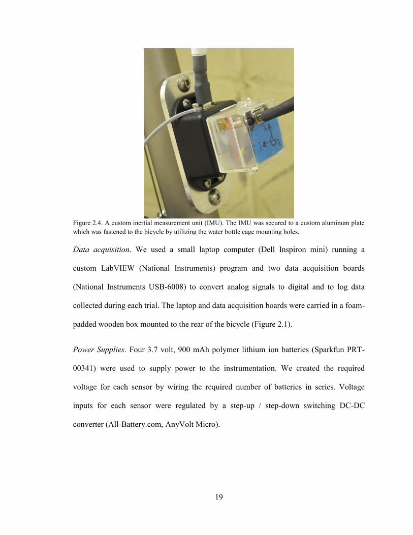
Figure 2.4. A custom inertial measurement unit (IMU). The IMU was secured to a
custom aluminum plate which was fastened to the bicycle by utilizing the water bottle
cage mounting holes. ........................................................................................................ 19
Figure 3.1. Identification of a region of steady-state turning. Bicycle speed, roll rate,
steering angle, and instantaneous turn radius were used to identify a region of steady-state
turning for processing. The region of steady turning for the example trial shown (a
medium speed, clockwise turn with a turn radius of 9.14 meters) lies within the two
vertical (black) lines. Another large region of steady-state turning begins around 90
seconds and ends at approximately 125 seconds. The turn radius data has been truncated
to highlight the steady-state turning region of interest. .................................................... 26
Figure 3.2. (A) The rotation of the bicycle-fixed frame )ˆ,ˆ,ˆ( kji eee relative to the sensor-
fixed frame )ˆ,ˆ,ˆ( 321 eee . (B) The rotation of the bicycle-fixed frame relative to the inertial
frame )ˆ,ˆ,ˆ( ZYX eee . (C) A sketch of a bicycle showing the relationship of the sensor-fixed
frame )ˆ,ˆ,ˆ( 321 eee to the conventional vehicle dynamics coordinate system ),,( ZYX when
the bicycle is in the upright position. Note that )ˆ,ˆ,ˆ( ZYX eee is aligned with ),,( ZYX . .... 28
Figure 3.3. A jig was used to validate our method of estimating the bicycle roll angle by
allowing us to orient the inertial measurement (IMU) at a fixed simulated roll angle. The
simulated roll angle was independently measured using an inclinometer that can resolve
the roll angle to within 0.01 degrees (inset photograph). The jig was secured to a
bicycle trailer and pulled behind the instrumented bicycle on level pavement. The white
rectangle indicates the location of the IMU on the jig secured to the trailer. ................... 30

xii
Figure 3.4. Bicycle roll angle versus normalized lateral acceleration. The experimental
data are predicted well by the model (slope = 1.00, R2 = 0.956). Deviation from the
model prediction can be interpreted as additional roll of the bicycle caused by a lateral
shift in the bicycle/rider system center of mass. Positive values of lateral acceleration
correspond to clockwise turns; negative values correspond to counter-clockwise turns.
Note that the model predicted bicycle roll angle is nearly linear in lateral acceleration; the
non-linear effects for the experimental conditions are contained within the width of the
plotted line. ....................................................................................................................... 37
Figure 3.5. Measured steering angle versus model predicted steering angle. The
experimental data are predicted well by the model (slope = 0.96, R2 = 0.995). The
clusters of data correspond to the different radii of turns tested experimentally. Scanning
from left to right, the data groups correspond to: counter clockwise turning around radii
of approximately 12.2, 18.3, 28.0 and 32.5 meters and clockwise turning around turns of
22.9 and 9.1 meters. .......................................................................................................... 39
Figure 3.6. Measured steering torque versus the model predicted steering torque. The
linear fit of the measured values to the model changes appreciably with different rider-
lean conditions. The model provides a good fit to the ‘normal riding’ condition (slope =
0.86, R2 = 0.566), but provides poor fits to the ‘rider lean into turn’ (slope = -1.33, R
2 =
0.155) and ‘rider lean out of turn’ (slope = 3.98, R2 = 0.634) conditions. ....................... 40
Figure 3.7. The ratio of steering torque to steer angle versus bicycle speed squared. A
negative ratio means that a rider must apply a counter-clockwise (negative) steering
torque when applying a clockwise (positive) steer angle, whereas a positive ratio means
that a rider must apply a clockwise (positive) steering torque when applying a clockwise
(positive) steer angle. Both riders were able to significantly change the ratio by leaning
into or out of a turn. .......................................................................................................... 42
Figure 3.8. The ratio of bicycle roll angle and steering angle versus bicycle speed
squared. Both subjects were able to significantly change the y-intercept of a linear fit to
the data by leaning into or out of a turn. ........................................................................... 44
Figure 4.1. An adapted bicycle. The adapted bicycles used by Lose the Training Wheels
utilize crowned rollers in place of a rear wheel. The roller is driven by a belt, which is
driven by a pulley connected to a standard bicycle transmission. In addition, the bicycles
also have a handle attached to the rear of the bicycle that allows a trainer to assist the
rider as needed. For this study, three wireless inertial measurement units (IMUs) were
mounted the bicycles: one on the frame (frame mounted IMU), another on the handlebar
stem (stem mounted IMU), and one on the spokes of the front wheel (wheel mounted
IMU). ................................................................................................................................ 57
Figure 4.2. The rollers used on the adapted bicycles. A series of crowned rollers is used
to modify the characteristics of the adapted bicycle. Roller number 1 (top) has the
smallest crown (less lean/greater stability) while roller number 8 (bottom) has the largest
crown (most lean/least stability). Participants often begin with roller number 3 and end
with roller number 6 before advancing to a traditional bicycle. ....................................... 58

xiii
Figure 4.3. The sensor-fixed and bicycle-fixed frames. Measurements in the sensor-fixed
frames 321ˆ,ˆ,ˆ eee and 654
ˆ,ˆ,ˆ eee must be resolved in bicycle-fixed frames relevant to
understanding bicycle dynamics; kji eee ˆ,ˆ,ˆ for roll/lean motion and nml eee ˆ,ˆ,ˆ for steer
motion. The rotation angles and are used to align the sensor-fixed frame 321ˆ,ˆ,ˆ eee
with the bicycle-fixed frame
kji eee ˆ,ˆ,ˆ . The steer axis tilt angle, , is used when resolving
the steer rate. The frame 654ˆ,ˆ,ˆ eee is not always exactly equal to nml eee ˆ,ˆ,ˆ due to
potential slight misalignment of the two frames. .............................................................. 62
Figure 4.4. Peak cross-correlation squared ( 2R ) between steer and roll angular velocities
versus training day/time for each subject (labeled A-O). Results of riders who learned to
ride a traditional bicycle are plotted in black, whereas those who did not are plotted in
gray. Dots signify trials on adapted bicycles whereas open circles signify trials on
traditional bicycles. The peak cross-correlation significantly increased with training time
(F = 44.203, p < 0.001). .................................................................................................... 70
Figure 4.5. Mean peak cross-correlation squared ( 2R ) between steer and roll angular
velocities of those who learned to ride versus those that did not. The error bars represent
± one standard deviation. Riders who learned to ride a traditional bicycle exhibited a
significantly higher correlation between steer and roll angular velocities than riders who
did not learn (t = 5.434, p = 0.003). .................................................................................. 71
Figure 4.6. Slope of the linear fit of steer angular velocity to roll angular velocity at the
time shift required for peak correlation versus training time. Plots for individual riders
(labeled A-O) are provided to illustrate change as riders progressed through the camp.
The results of riders who learned to ride a traditional bicycle are plotted in black, whereas
the results of riders who did not are plotted in gray. Trials in which the rider rode a
traditional bicycle are plotted with a circle. The slope significantly increased with
training time (F = 31.931, p < 0.001). ............................................................................... 71
Figure 4.7. Standard deviation of the steer angular velocity versus training time. Plots for
individual riders (labeled A-O) are provided to illustrate change as riders progressed
through the camp. The results of riders who learned to ride a traditional bicycle are
plotted in black, whereas the results of riders who did not are plotted in gray. Trials in
which the rider rode a traditional bicycle are plotted with a circle. The standard deviation
of the steer rate increased significantly over time for all trials (F = 27.579, p < 0.001) and
for the subset of trials on the adapted bicycles (F = 25.196, p < 0.001). .......................... 73
Figure 4.8. Standard deviation of the roll angular velocity versus training time. Plots for
individual riders (labeled A-O) are provided to illustrate change as riders progressed
through the camp. The results of riders who learned to ride a traditional bicycle are
plotted in black, whereas the results of riders who did not are plotted in gray. Trials in
which the rider rode a traditional bicycle are plotted with a circle. The standard deviation
of the roll rate increased significantly over time for all trials (F = 30.254, p < 0.001) and
for the subset of trials on the adapted bicycles (F = 8.238, p = 0.008). ............................ 74
xiv
Figure 5.1. A cyclist riding a bicycle on rollers. ............................................................... 86
Figure 5.2. A platform placed over the rollers allows subjects to safely dismount the
bicycle and a railing beside the rollers allows subjects to support themselves during trials.
The roller drums are mounted to a frame that is attached to a force platform near the
center of the assembly. ...................................................................................................... 88
Figure 5.3. Three markers (1, 2, and 3) are attached to a rigid plate (black) which is fixed
to the headtube of the bicycle. .......................................................................................... 90
Figure 5.4. Relationship of the bicycle to the inertial frame. The inertial frame ),,( ZYX
is fixed to the force platform. The dashed line tangent to the rear wheel represents the roll
axis of the bicycle. ............................................................................................................ 91
Figure 5.5. The custom rollers. ......................................................................................... 93
Figure 5.6. The custom rollers. ......................................................................................... 93
Figure 5.7. The rollers are designed to be bolted to a force platform. Four brackets on the
base of the rollers are used to secure the rollers to the force platform using four bolts. .. 93
Figure 5.8. The front roller can be adjusted to ensure that the bicycle is level (adjustment
up and down) and to ensure that the roller contacts the front tire appropriately
(adjustment fore and aft). .................................................................................................. 94
Figure 5.9. A photograph of the instrumented bicycle on the custom rollers. Note that the
bicycle is leaning against the wall to stay upright. ........................................................... 94
Figure 5.10. Rider lean as viewed from behind the bicycle/rider. The rider lean angle
quantifies how a rider is shifting his/her center of mass relative to the bicycle. The arrows
define the positive sense of all angles. Rider lean )( lean is defined as the center of mass
roll angle )( COM minus the bicycle roll angle )( . For the example illustrated, the rider
lean angle is negative. ..................................................................................................... 100
Figure 5.11. Lateral (y) center of pressure location and center of mass location versus
time. Data from a representative trial (non-cyclist, 7.46 m/s) demonstrates the lateral
center of mass location closely tracks the lateral center of pressure location during
bicycle riding. ................................................................................................................. 104
Figure 5.12. Cross-correlation of the lateral position of the center of mass to the center of
pressure versus speed. The cross-correlation decreases significantly with increasing speed
(F = 29.113, p < 0.001) and decreases significantly more with increasing speed for non-
cyclists than cyclists (F = 14.843, p < 0.001). ................................................................ 105
Figure 5.13. Slope of the linear fit of the lateral position of the center of mass to the
center of pressure versus speed. The slope decreases significantly with increasing speed

xv
(F = 11.352, p = 0.001) and decreases significantly more for non-cyclists than cyclists (F
= 11.263, p = 0.001). ....................................................................................................... 106
Figure 5.14. Bicycle roll rate and steer rate versus time. Data from a representative trial
(non-cyclist, v 7.96 m/s) demonstrates that the steer rate ( ) lags and is correlated to
the bicycle roll rate ( ) during riding. ............................................................................ 107
Figure 5.15. Cross-correlation of steer rate to bicycle roll rate versus speed. The cross-
correlation decreases significantly with increasing speed (F = 34.307, p < 0.001) and
decreases significantly more with increasing speed for cyclists than non-cyclists (F =
4.650, p = 0.035). ............................................................................................................ 108
Figure 5.16. Slope of the linear least-squares fit of steer rate to bicycle roll rate versus
speed. The slope decreases significantly with increasing speed (F = 142.123, p < 0.001).
There are no significant differences between cyclists and non-cyclists. ........................ 109
Figure 5.17. Standard deviation of steer angle versus speed. The standard deviation of
steer angle decreases significantly with increasing speed (F = 114.264, p < 0.001).
Cyclists exhibit significantly less steer angle variation than non-cyclists (F = 13.904, p <
0.001). ............................................................................................................................. 110
Figure 5.18. Average positive steering power versus speed. All riders produce less
positive power to steer the bicycle as speed increases (F = 10.547, p = 0.002). Cyclists
produce less positive power than non-cyclists (F = 19.213, p < 0.001). ........................ 111
Figure 5.19. Bicycle roll angle and rider lean angle versus time. Data from a
representative trial (cyclist, v 2.526 m/s) demonstrates that rider lean ( lean ) is highly
correlated with and opposite to the bicycle roll angle ( ). Refer to Figure 5.10 for
definitions of lean and . ............................................................................................... 112
Figure 5.20. Cross-correlation of rider lean angle to bicycle roll angle versus speed. The
cross-correlation decreases significantly with increasing speed (F = 32.948, p < 0.001)
and decreases significantly more with increasing speed for non-cyclists than cyclists (F =
17.639, p < 0.001). .......................................................................................................... 113
Figure 5.21. Slope of the linear least-squares fit of rider lean angle to bicycle roll angle
versus speed. The magnitude of the slope decreases significantly with increasing speed (F
= 19.220, p < 0.001) and decreases significantly more with increasing speed for non-
cyclists than cyclists (F = 13.865, p < 0.001). ................................................................ 114
Figure 5.22. Standard deviation of rider lean angle versus speed. Cyclists exhibit
significantly less rider lean than non-cyclists (F = 19.643, p < 0.001). .......................... 115
Figure 5.23. Standard deviation of the lateral position of the center of pressure versus
speed. The standard deviation of the lateral position of the center of pressure decreases
significantly with increasing speed (F = 25.294, p < 0.001). Although it may appear that

xvi
cyclists exhibit less variation in the center of pressure position than non-cyclists, there
was not a significant difference between the two groups (F = 3.695, p = 0.059). .......... 117
xvii
LIST OF TABLES
Table 3.1. Differences between the estimated bicycle roll angle and the model predicted
roll angle for different lean conditions. A positive value indicates that a rider can increase
the magnitude of the bicycle roll angle by leaning, whereas a negative value indicates that
rider can decrease the magnitude. ..................................................................................... 37
Table 3.2. Summary of the linear fit )( bmxy of measured values to model predicted
values. ............................................................................................................................... 38
Table 3.3. Summary of the linear fit bvmT )()/( 2 . ................................................ 42
Table 3.4. Summary of the linear fit bvm )()/( 2 . ................................................. 43
Table 4.1. Subject details. ................................................................................................. 55
Table 5.1. Comparison of kinematic-based and kinetics-based estimates of center of mass
location and acceleration................................................................................................... 98
Table 5.2. Summary of statistical tests. Significant effects are denoted with an asterisk
(*). ................................................................................................................................... 103
Table A.1. Body segment properties (from Clauser et al. [136] and Dempster [128]). The
mass of each segment is calculated as a fraction of the body mass and the location of the
center of mass of each segment is calculated as a fraction of the segment length. ........ 140
Table A.2. Bicycle parameters for use in the model. ...................................................... 145

xviii
ABSTRACT
An Experimental Investigation of Human/Bicycle Dynamics and Rider Skill in Children
and Adults
by Stephen Matthew Cain
Chair: Noel C. Perkins
While humans have been riding bicycles for nearly 200 years, the dynamics of how
exactly they achieve this are not well understood. The overall goals of this dissertation
were to identify the major control strategies that humans use to balance and steer
bicycles, as well as to identify performance metrics that reliably distinguish rider skill
level. To achieve these goals, we introduced: a) a novel instrumented bicycle to measure
rider control inputs and bicycle response outputs, b) an experimental design and
analytical approach for tracking and quantifying rider learning, and c) an experimental
design and analytical approaches to measure the dynamics of human/bicycle balance and
quantify rider balance performance. We employed variations of the instrumented bicycle
in three studies that focused on: 1) how adult riders control bicycle kinematics during
steady-state turning, 2) the initial learning of steering and balance control as children
learn to ride bicycles, and 3) the balance skill of adult expert and novice riders.

xix
The findings from these studies advance our understanding of the types of control used
by human riders, and simultaneously, quantify rider learning and skill. During steady-
state turning, rider lean strongly influences steering torque, suggesting that rider lean
plays an important role in bicycle control. Children learned to ride after successfully
learning how to steer in the direction of bicycle roll, thereby increasing the correlation
between steer and bicycle roll angular velocities (coefficient of determination increased
from 0.22 to 0.75 during the learning process). In adults, the superior balance
performance of skilled versus novice riders is revealed by highly correlated lateral
positions of the center of pressure and center of mass (coefficients of determination of
0.97 versus 0.89, respectively). In achieving their superior balance performance, skilled
riders employed more rider lean control, less steer control, and used less control effort
than novice riders. We conclude that rider lean (i.e., any lateral movements of the rider)
plays a dominant role in both steering and balancing a bicycle, and that achieving balance
requires coordinating both steer and rider lean (the two rider control inputs) with bicycle
roll (the bicycle response).

1
CHAPTER 1: MOTIVATION, LITERATURE REVIEW, AND RESEARCH OBJECTIVES
1.1 Motivation
Humans have ridden bicycles (two-wheeled, single track vehicles) since the early 1800’s
[1], yet human/bicycle dynamics are far from well understood. Recent work [2] has
established the so-called Whipple bicycle model [3] as the simplest model of a bicycle
that can predict the self-stability of an uncontrolled bicycle. By contrast, there is still little
understanding of the fundamental characteristics of human riders, the types of control
that humans use, and the skills that distinguish riders of different ability levels.
Understanding rider learning and skill could help to improve programs that teach affected
populations to ride, such as Programs to Educate All Cyclists1
(PEAC) and Lose the
Training Wheels2 and provide a way to objectively measure whether a specific bicycle is
better or worse for a particular rider.
1.2 Background
Stability of an Uncontrolled Bicycle and the Whipple Model 1.2.1
The dynamics of an uncontrolled bicycle, either without a rider or with a rigid but non-
actuating rider, are well understood. The relatively recent work by Meijaard et al. [2]
presents complete equations of motion for what is referred to as the Whipple bicycle
model. The authors also present bicycle parameters that can be used for benchmarking
1 www.bikeprogram.org
2 www.losethetrainingwheels.org

2
and a thorough review of the bicycle dynamics literature, arguing that no prior journal
publication in English presents complete and correct equations for the Whipple model.
The Whipple bicycle model consists of four rigid bodies: a rear wheel, a rear frame with
a rider rigidly attached to it, a front frame consisting of the front handlebar and fork
assembly, and a front wheel. The model assumes that all bodies are laterally (left-right)
symmetric and that the wheels have circular symmetry. Motion of the rider relative to the
frame, structural compliance and damping, joint friction, and tire compliance and slip are
neglected. Tire contacts with the ground are approximated by knife-edge rolling point-
contacts. The model is described by seven generalized coordinates. As noted in [2], only
three of the generalized coordinates are independent upon accounting for four non-
holonomic rolling constraints. After linearizing the model about upright, straight-line
motion and treating forward speed as a parameter, the model is reduced to two
generalized coordinates; namely the steer angle and the lean (or roll) angle. The model
successfully explains the observed self-stability of an uncontrolled bicycle (within a
specific speed range) and the coupling between lean and steer.
Extensions of the Whipple model have been proposed to investigate added complexities
for an uncontrolled bicycle. Meijaard and Schwab [4] expanded the Whipple model to
include the effects of tire shape, a linear tire model, road gradient, and driving and
braking torques. Sharp [5] investigated acceleration, finite cross-section tires, tires as
force and moment generators, tire dynamics, frame compliance, and rider compliance.
Peterson and Hubbard [6] and Schwab et al. [7], among others, added an additional
degree of freedom to allow rider lean relative to the bicycle. Schwab and Kooijman [8]
investigated the effects of coupling between the passive rider and the bicycle. All of these

3
additional effects lead to different open-loop dynamics—however, these differences are
also relatively minor.
The Whipple bicycle model is useful for predicting the stability of real bicycles.
Kooijman et al. demonstrated that the eigenvalues predicted by the Whipple model are in
good agreement with the experimentally measured eigenvalues for a riderless bicycle
both overground [9] and on a treadmill [10]. In [11], Kooijman et al. used the Whipple
bicycle model to design a self-stable bicycle with no gyroscopic effects or trail (also
known as caster [11]), which are two properties of typical bicycles that were thought to
be essential for a bicycle to be self-stable. These studies demonstrate that the Whipple
model is sufficient for understanding the stability and open-loop dynamics of bicycles.
Under the assumption that the open-loop dynamics of a bicycle relate to “rideability” or
maneuverability of the bicycle, a number of studies investigated how changes in
parameters affect bicycle stability. Moore and Hubbard [12] investigated the effects of
front wheel diameter, steer axis tilt (or head tube angle), trail, and wheelbase on the range
of stable speeds predicted by the Whipple model. Tak et al. [13] performed a sensitivity
analysis on the range of stable speeds with respect to changes in all 25 bicycle parameters
and found that head tube angle had the greatest effect on stability. Not surprisingly, real
bicycles are not designed to be as stable as possible—they must also be easily
maneuverable [14].
Human Control of Bicycles 1.2.2
Sheridan and Ferrell in their book about man-machine systems [15] state that “…the
quality of performance of either the human or the machine component by itself does not

4
determine the quality of system performance.” The quality of a bicycle cannot be
determined from only looking at the bicycle’s open loop dynamics. Throughout the
history of the bicycle, humans have demonstrated that they are capable of successfully
riding a wide range of bicycle designs, including bicycles that have no self-stability. In
fact, early bicycles likely had very little self-stability, as they had vertical steering axes
and little to no trail [1]. Researchers also set out to design bicycles with no self-stability
[16] and bicycles that are “unrideable” [17, 18]; however, such bicycles have proven to
be easily rideable [16, 17] or rideable after practice. In addition, even bicycles that are
self-stable are only self-stable for a limited range of speeds; outside of the limited speed
range the bicycles must be stabilized by human control. Therefore, understanding the
human rider and the control that a rider uses are important for understanding bicycles and
bicycle design.
Researchers have modeled human control of bicycles as a steering torque (applied by a
rider through the handlebars) and a leaning torque (applied by a rider by leaning relative
to the bicycle) [6, 7, 19]. These control inputs are similar to those considered in the study
of motorcycles [20-22]. However, the ratio of rider mass to vehicle mass is much greater
for a bicycle rider than for a motorcycle rider, which makes other and more subtle control
possible. For example, experimental observations of human control reveal that human
riders may use lateral knee movements and more complex upper body movements,
especially at lower speeds [23, 24]. A number of studies have investigated automatic or
robot control of a bicycle [25-29], and reveal that human-like control (steering angle and
simulated rider lean) as well as control schemes not accessible to humans (gyroscopic
stabilization) can successfully keep a bicycle upright. These studies highlight the fact that

5
a human rider (or robot rider) has many ways of controlling and balancing a bicycle—yet
not all of these control movements are easy to model or measure.
As expected, a wide range of controllers successfully stabilize and steer bicycle models.
These controllers include: steer-into-the-lean (intuitive) model [7], linear quadratic
regulator [7], cross-over control model [30], optimal linear preview [19], among others
[6, 31, 32]. However, the primary goal of these controllers has been to evaluate bicycle
design. For example, Schwab et al. [7] investigate the gains that must be used by the
controller; Sharp [19] quantifies the preview time necessary to achieve certain levels of
performance with a given bicycle design; and, Hess et al. [30] quantify the handling
qualities of bicycles using a handling qualities metric originally proposed for evaluating
aircraft. However, none of these controllers were developed with the idea of investigating
the performance of the human rider.
Researchers used various forms of system identification to solve for parameters of
modeled controllers. Work by van Lunteren and Stassen [33] utilized a bicycle simulator
instead of a real bicycle and revealed that controller parameters can be quite variable both
for different trials with the same rider and between different riders. Preliminary work by
Moore [34] demonstrates similar findings. Therefore, it is not clear how control
parameters might be correlated with rider skill or performance.
Assessing Rider Skill/Performance 1.2.3
Bicycle riding skill or performance has previously been assessed by instructing subjects
to ride around a prescribed course or to perform a prescribed task. In general, the time to
complete a course/task and the number of errors committed are used to quantify

6
performance. In the majority of studies that use these techniques, the goal has been to
evaluate the performance or safety of a particular bicycle or bicycle configuration [35-
40]. In a study investigating the maneuverability of children’s bicycles [40], Lewis noted
that there was more variation between subjects than between the use of different bicycles.
The time to complete a course and number of errors were used to investigate the
correlation between physical and perceptual-motor abilities and riding performance [41,
42] and to evaluate the effect of alcohol consumption on the ability to safely ride a
bicycle [43]. While quantifying performance by time to complete a course/task and the
number of errors is useful for the questions posed in the previously mentioned studies,
the results from these studies are task specific and do not translate to new tasks. In
addition, the methods of quantifying performance do not allow continuous monitoring of
skill because the methods rely on completion of specific courses/tasks. The methodology
is also not useful if it is not possible for a rider to complete a task; for example, a child
that has not yet learned to ride a bicycle would not be able to successfully ride around a
course.
Some motorcycle research suggests that riders of different skill levels use different body
lean relative to the motorcycle and steering torque. For example, Rice [44] found that
riders of different skill levels phased body lean and steering torque differently when
executing a lane change maneuver. Similarly, Prem [45] found that novice riders in an
evasive maneuver used lean torque and steering torque differently from expert riders.
Prem also used skill tests to differentiate rider ability, similar to the bicycle studies
mentioned above. However, these studies also provide little insight on how to
continuously monitor skill or motor learning for bicycle riders.

7
In the absence of quantitative tools to evaluate rider learning and rider skill, researchers
and programs that teach children how to ride must resort to qualitative assessments. For
example, the Lose the Training Wheels3 program uses specially trained floor managers to
observe riders who determine if the rider is learning. The floor manager observes the
speed of pedaling, whether a rider leans into turns, relaxes his/her arms and uses the
handlebars to turn and control the bicycle [46]. However, it is unclear how these
qualitative assessments correlate to riding skill. A quantitative measure of skill would
allow bicycle programs to monitor rider progress more effectively and potentially create
better methods to teach bicycle riding.
Human Balance Skill 1.2.4
The ability to balance the bicycle is necessary to successfully complete any riding task.
Therefore, it seems logical to investigate possible ways to quantitatively evaluate the skill
or ability of a rider to balance. Other fields of research have investigated human
balancing skills and performance and these provide insight into how bicycle balancing
skill could be quantified. Two such fields are human postural control and human walking.
1.2.4.1 Human standing balance
The tools used to evaluate human postural control are an essential part of both clinical
evaluation of patients and research into how humans maintain upright posture. Some of
the most basic methods used to evaluate human postural control involve monitoring the
location of the center of pressure (COP) and the center of mass (COM) [47]. By using an
ideal inverted pendulum model of standing balance, Winter [47] explains that the (COP-
COM) signal is directly related to the horizontal acceleration of the COM and can be
3 www.losethetrainingwheels.org

8
considered to be the error signal detected by the balance control system. The assumption
is that the goal of the balance control system is to maintain an upright posture and to
control postural sway. While it is assumed that human standing balance can be modeled
effectively as an inverted pendulum, it is important to note that more complex balancing
tasks cannot be explained by this simple approach and require a more complex model of
the body [48]. Researchers have used COP measurements to investigate standing balance
using a wide range of statistics, including: root mean square (RMS) distance from the
mean COP [49, 50], excursions of the COP [51-53], COP sway amplitude [54], velocity
of the COP [55, 56], and the area enclosed by the COP trajectory [55, 57], among others.
More advanced methods of quantifying balance performance have investigated the
frequency content of the COP movement [56], the relationship of the COP to the COM
movement [47], and the relationship of the COP and/or COM movement to muscle
activation patterns [52, 58]. Researchers have also used system identification techniques
to identify various transfer functions for standing balance [59, 60]. Depending on the
experimental protocol, identified system parameters or attributes can be used to
understand the controller or plant during standing balance [61, 62]. However, there is not
yet a clear way to use these measures for diagnosing balance disorders [63, 64].
Basic quantitative measures of postural control identify at risk populations and
differences in balance performance. Maki et al. [49] demonstrated that postural sway, as
measured by COP displacement, is correlated with future falling risk. Prieto et al. [57]
found that the mean velocity of the COP signals differences between healthy young and
elderly adults and differences between eyes-open and eyes-closed standing balance
conditions. Pellecchia [50] demonstrated that postural sway, as measured by movement
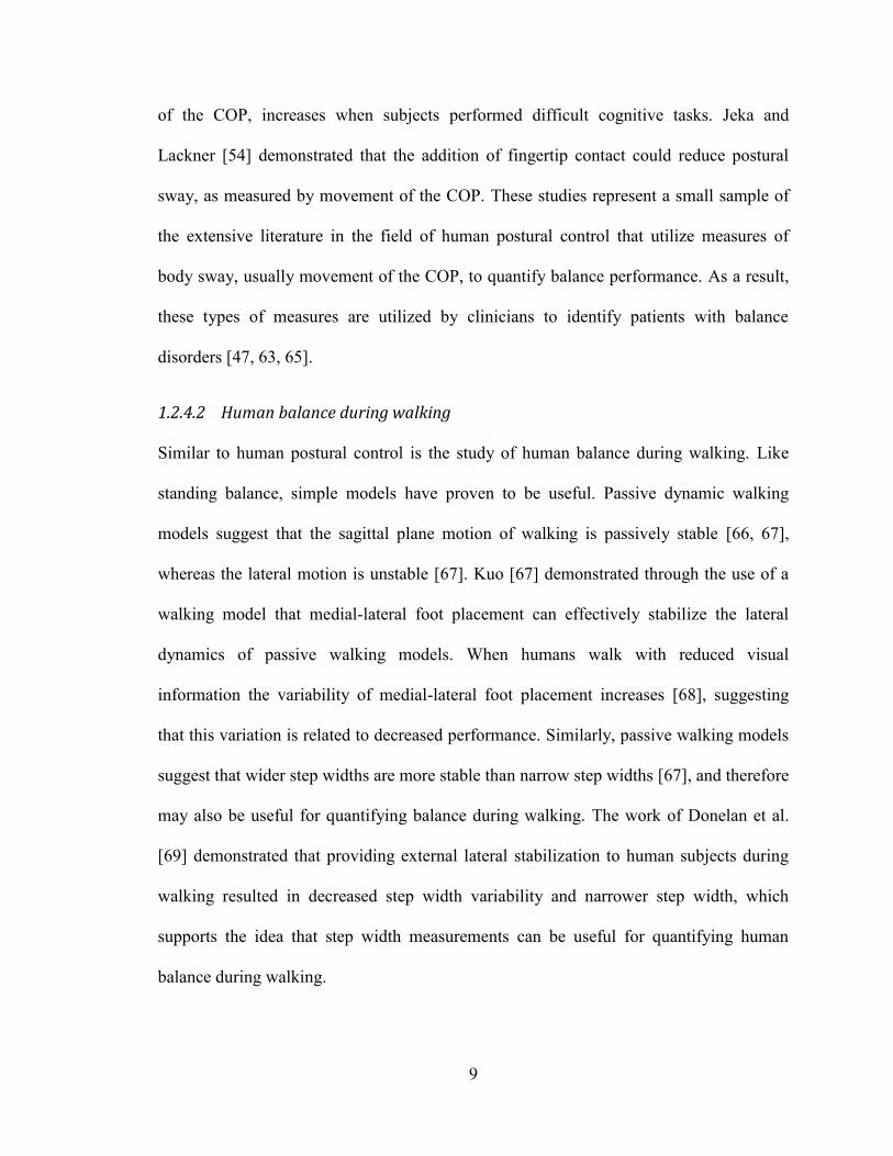
9
of the COP, increases when subjects performed difficult cognitive tasks. Jeka and
Lackner [54] demonstrated that the addition of fingertip contact could reduce postural
sway, as measured by movement of the COP. These studies represent a small sample of
the extensive literature in the field of human postural control that utilize measures of
body sway, usually movement of the COP, to quantify balance performance. As a result,
these types of measures are utilized by clinicians to identify patients with balance
disorders [47, 63, 65].
1.2.4.2 Human balance during walking
Similar to human postural control is the study of human balance during walking. Like
standing balance, simple models have proven to be useful. Passive dynamic walking
models suggest that the sagittal plane motion of walking is passively stable [66, 67],
whereas the lateral motion is unstable [67]. Kuo [67] demonstrated through the use of a
walking model that medial-lateral foot placement can effectively stabilize the lateral
dynamics of passive walking models. When humans walk with reduced visual
information the variability of medial-lateral foot placement increases [68], suggesting
that this variation is related to decreased performance. Similarly, passive walking models
suggest that wider step widths are more stable than narrow step widths [67], and therefore
may also be useful for quantifying balance during walking. The work of Donelan et al.
[69] demonstrated that providing external lateral stabilization to human subjects during
walking resulted in decreased step width variability and narrower step width, which
supports the idea that step width measurements can be useful for quantifying human
balance during walking.

10
The basic methods of quantifying the lateral dynamics of human walking are useful for
assessing balance during human walking. Variability of step width remains a good
predictor of falling in the elderly [70-72] that can be used in a clinical setting. Applying
external lateral stabilization to subjects with myelomeningocele allows them to walk with
decreased step width and decreased medial-lateral motion of the COM [73]. Given the
ability to quantify balance skill, researchers investigated the use of physical guidance and
error augmentation to affect the motor learning of human subjects walking on a narrow
beam [74, 75].
1.3 Relationship of bicycle riding to other human balancing tasks
Both standing and walking require maintaining a specific relationship between the center
of mass of the body and the base of support. In static situations, the vertical projection of
the center of mass should fall within the base of support. However for dynamic situations,
this description is insufficient [76, 77]. In dynamic balancing tasks, both center of mass
position and velocity must be considered to understand balance limits [76-78].
Riding a bicycle is similar to standing and walking in that it requires the human to
maintain balance. Instead of maintaining the center of mass of the body within some
margin of the base of support, a bicycle rider must maintain the center of mass of the
bicycle/rider system within some limits of the base of support defined by the contact of
the bicycle tires with the ground. Most likely these limits are a function of the bicycle
speed and yaw rate, which are important for understanding the lateral acceleration and
thus the roll angle of a single track vehicle [79]. As discussed in Sections 1.2.4.1 and
1.2.4.2, dynamic measurements such as the center of pressure position/velocity, center of
mass position/velocity, and step width can be useful for evaluating stability or balance
11
performance during standing and walking tasks. Unlike standing and walking, it is
unclear how dynamic measures of the bicycle/rider system might be related to stability or
balance performance. Bicycle riding is also unlike standing and walking in that the rider
must control more than just his/her body. In addition to applying joint torques to alter
body posture (as in standing balance [48, 80]), a bicycle rider can also steer the bicycle to
maintain balance. Analyses of rider motion reveal that riders use both lateral body
movements and steering while riding [24], but it remains unclear which rider motions are
essential for balance.
1.4 Research Objective and Specific Aims
Following the above review of human/bicycle dynamics and rider skill, the overall
objectives of this dissertation are to: 1) understand how humans balance and steer
bicycles, and 2) quantify the skill of human riders. To meet these objectives, the
following specific aims are pursued:
1. Design and build an instrumented bicycle that is capable of measuring the
primary human control inputs (steer torque and rider lean) and fundamental
bicycle kinematics.
2. Investigate human/bicycle dynamics and control during steady-state turning
using experimental and analytical approaches.
3. Quantify the changes that occur as learners transition from non-riders to
riders.
4. Quantify the differences between skilled and novice riders when balancing a
bicycle.
12
In Chapter 2 (specific aim 1) we describe and document the instrumented bicycle. In
Chapter 3 (specific aim 2) we discuss our investigation of steady-state turning, in which
we employ the instrumented bicycle to make experimental measurements and present a
steady-state turning model to interpret our results. Specific aim 3 is addressed by Chapter
4, in which we describe results from our study that uses measured bicycle kinematics to
quantify rider learning as novice riders with disabilities progress through a specialized
bicycle camp. Differences between skilled and novice riders (specific aim 4) are
quantified in Chapter 5.

13
CHAPTER 2: DEVELOPMENT OF AN INSTRUMENTED BICYCLE
2.1 Chapter Summary
In this chapter we describe the design of an instrumented bicycle. The instrumented
bicycle is capable of measuring steering torque (the primary human control), bicycle
speed, steering angle, acceleration of the bicycle frame, and angular velocity of the
bicycle frame. Using the methodology discussed in Chapter 3 Section 3.3.2, it is possible
to resolve the bicycle roll angle and the additional roll of the bicycle caused by rider lean
relative to the bicycle frame for steady turning of a bicycle. As later discussed in Chapter
5, the instrumented bicycle can also be used to resolve the roll and yaw rates of the
bicycle frame and to quantify the amount of work done by a rider to balance a bicycle.
We begin this chapter with a brief review of other instrumented bicycles, and then
describe the instrumentation and data acquisition system. The content of this chapter also
appears in a published conference paper [81] and a published journal article [82].
2.2 Brief review of instrumented bicycles
Instrumented bicycles have been used to investigate the human control and dynamic
behavior of bicycles. Roland [31] instrumented a bicycle to measure the rider lean angle
and the steering angle, roll angle and speed of the bicycle in order to verify simulation
results of a riderless bicycle and to analyze the steer and lean control used by a human
rider. Jackson and Dragovan [83] instrumented a bicycle to measure the steering angle,
speed and angular velocity of the bicycle during no-hands riding in conjunction with

14
simplified equations of motion to understand the torque applied to the front wheel by the
ground reaction force and the gyroscopic moment. Cheng et al. [84] instrumented a
bicycle to measure steering torque and confirm that larger torques are required to initiate
turns with larger steering angles. Kooijman et al. [9] instrumented a riderless bicycle for
angular rates, steering angle, and speed to validate a model of an uncontrolled bicycle at
low speeds. More recently, Kooijman and Schwab [23] instrumented a bicycle for roll,
yaw, and steering rates, steering angle, rear wheel speed, pedaling cadence as well as
video capture of rider motion. They conclude that during normal cycling, most rider
control is imparted through steering as opposed to upper body lean.
2.3 Description of the instrumented bicycle
An instrumented bicycle was constructed to measure the primary human control used by
a human rider (steer torque) and the most relevant bicycle kinematics. In the following,
we describe the bicycle, the sensors, the power supplies, and the data acquisition system.
Bicycle 2.3.1
The bicycle shown in Figure 2.1 is a standard geometry (steer axis tilt = 18.95 degrees,
trail = 64 mm, wheel base = 1.060 m), rigid (unsuspended) mountain bike (1996 Schwinn
Moab 3, size 19 inch frame) equipped with 660.4 mm x 49.5 mm (26 in x 1.95 in) slick
tires (Tioga City Slicker 26 x 1.95, ETRTO 48-559). The wheel bearings were properly
adjusted and the wheels were trued by a professional bicycle mechanic prior to testing.
To accommodate the torque sensor, the stock fork was replaced with an aftermarket rigid
(unsuspended) fork (Surly 1x1, 413 mm axle-to-crown length, 45 mm rake/offset).

15
Figure 2.1. The instrumented bicycle. The instrumented bicycle is a standard geometry mountain bike
equipped to measure: steering torque, steering angle, bicycle speed, bicycle angular velocity about three
axes, and acceleration along three axes. A laptop computer, A/D boards, battery, and circuitry are
supported in a box at the rear.
Instrumentation 2.3.2
The instrumentation selected for this study enables the simultaneous measurement of the
steering torque, the steering angle, the bicycle speed, and the acceleration and angular
velocity of the bicycle frame as described below.
Steering torque. We constructed the custom instrumented fork shown in Figure 2.2 to
measure the steering torque. The placement of a torque sensor (Transducer Techniques
SWS-20) within the steerer tube permitted the measurement of the torque transmitted
between the handlebars and the front wheel. We isolated the torque sensor from
unwanted bending moments and axial loading by using angular contact bearings (Enduro
7901) in conjunction with the pair of angular contact bearings in the bicycle headset; the
bearings were preloaded prior to testing, similar to the way that a threadless headset is
adjusted. Following installation, we calibrated the torque sensor in situ by orienting the

16
bicycle such that the steering axis was parallel to the ground, securing a long length of
threaded rod in the fork dropouts, and then placing known masses at measured distances
from the steering axis to create known torques. Following calibration, we measured the
stiffness of the torque sensor to be 4.97 Nm/deg. The signal from the torque sensor was
amplified using a load cell signal conditioner (Transducer Techniques TMO-1) and was
sampled at 1000 Hz in the experiments described below. The range and resolution of the
torque measurements are +/- 7.512 Nm and 0.005 Nm, respectively.
Figure 2.2. The instrumented fork. We constructed a custom instrumented fork to measure steering torque.
(A) An exploded view of the steerer tube of the instrumented fork. (B) A section view of the assembled
instrumented fork. (C) A photograph of the disassembled instrumented fork.
Steering angle. We employed an optical encoder to measure the steering angle. We
secured a custom encoder disk (US Digital HUBDISK-2-1800-1125-I) to the bicycle fork
similar to a headset spacer as illustrated in Figure 2.3. We attached the encoder module

17
(US Digital EM1-2-1800) to a custom aluminum plate, which was secured to the bicycle
frame by using the top headset race as shown in Figure 2.3. An encoder chip (LSI/CSI
LS7183 in resolution mode) was used to convert the raw signal from the encoder
module to up and down counts and was sampled at 200 Hz, which is the maximum
sampling rate for a digital input to the data acquisition board. Due to the flexibility of the
steering assembly caused by the torque sensor, the steering angle is corrected as
described in Chapter 3 Section 3.3.2. The optical encoder measures the steering angle
with a resolution of 0.1 degrees.
Figure 2.3. The encoder and encoder disk used to measure the steering angle. The encoder module was
fastened to a custom aluminum plate secured to the bicycle frame using the upper headset cup. The encoder
disk was secured to the steerer tube of the fork, similar to a headset spacer.
Bicycle speed. We calculated the average bicycle speed for each revolution of the front
wheel by dividing the circumference of the front wheel by the time required for each
revolution. The circumference of the front wheel was calculated from the rolling radius of
the front wheel, which was measured as described in Section A.2 of Appendix A. Wheel
revolutions were measured using a magnetic reed switch (Cateye 169-9772) and a single
18
wheel mounted magnet (Cateye 169-9691). We sampled the signal from the magnetic
reed switch at 1000 Hz. Speed updates, obtained once per wheel revolution, translate to
update rates from 0.5 to 4.7 Hz for the bicycle speeds in our experiments. Assuming
resolutions of 0.001 seconds and 0.001 meters for the measured time for a wheel rotation
and wheel circumference, respectively, we estimate that the maximum error occurs at the
fastest speed (+/- 0.049 m/s or +/- 0.5%) and the minimum error occurs at the lowest
speed ( +/- 0.001 m/s or +/- 0.1%).
Acceleration and angular velocity. A custom inertial measurement unit (IMU) shown in
Figure 2.4 was constructed using a three-axis accelerometer (Analog Devices ADXL335)
and three single-axis angular rate gyros (Murata ENC-03M). We secured the IMU to a
custom aluminum plate which is fastened to the seat tube of the bicycle frame utilizing
the water bottle cage mounting holes (Figure 2.4). The angular velocity measurements
were used to calculate the turn radius and the acceleration measurements were used to
calculate the bicycle roll angle as further described in Section 3.3.2. The signals from the
accelerometer and three angular rate gyros were sampled at 1000 Hz. The IMU,
calibrated using the technique described by King [85], yields acceleration measurements
with a range and resolution of +/- 29.43 m/s2 and 0.067 m/s
2, respectively, and angular
velocity measurements with a range and resolution of +/- 300 deg/s and 3.04 deg/s,
respectively.
19
Figure 2.4. A custom inertial measurement unit (IMU). The IMU was secured to a custom aluminum plate
which was fastened to the bicycle by utilizing the water bottle cage mounting holes.
Data acquisition. We used a small laptop computer (Dell Inspiron mini) running a
custom LabVIEW (National Instruments) program and two data acquisition boards
(National Instruments USB-6008) to convert analog signals to digital and to log data
collected during each trial. The laptop and data acquisition boards were carried in a foam-
padded wooden box mounted to the rear of the bicycle (Figure 2.1).
Power Supplies. Four 3.7 volt, 900 mAh polymer lithium ion batteries (Sparkfun PRT-
00341) were used to supply power to the instrumentation. We created the required
voltage for each sensor by wiring the required number of batteries in series. Voltage
inputs for each sensor were regulated by a step-up / step-down switching DC-DC
converter (All-Battery.com, AnyVolt Micro).

20
CHAPTER 3: MEASUREMENT AND ANALYSIS OF STEADY STATE TURNING
3.1 Chapter Summary
The steady-state turning of a bicycle arises when the bicycle/rider system negotiates a
constant radius turn with constant speed and roll angle. This chapter explores steady-state
turning by employing the previously described bicycle instrumented to measure steering
torque, steering angle, and bicycle speed, acceleration, and angular velocity. We report
data obtained from 134 trials using two subjects executing steady turns defined by nine
different radii, three speeds, and three rider lean conditions. A model for steady-state
turning, based on the Whipple bicycle model, is used to interpret the experimental results.
Overall, the model explains 95.6% of the variability in the estimated bicycle roll angle,
99.4% of the variability in the measured steering angle, and 6.5% of the variability in the
measured steering torque. However, the model explains 56.6% of the variability in
steering torque for the subset of trials without exaggerated rider lean relative to the
bicycle frame. Thus, the model, which assumes a rigid and non-leaning rider, reasonably
predicts bicycle/rider roll and steering angles for all rider lean conditions and steering
torque without exaggerated rider lean. The findings demonstrate that lateral shifting of
the bicycle/rider center of mass strongly influences the steering torque, suggesting that
rider lean plays an important role in bicycle control during steady-state turning. By
contrast, the required steering angle is largely insensitive to rider lean, suggesting that the
steering angle serves as a superior cue for bicycle control relative to steering torque. The
experimental data presented in this chapter also appears in a published conference paper
21
[81] and a published journal paper [82]. The journal paper contains the same steady-state
model presented herein, whereas the conference paper presents a simplified model that
accounts for rider lean.
3.2 Background and organization of chapter
The design of the modern bicycle is the result of almost two centuries of trial and error.
Recent research has helped us understand the stability of a bicycle [2, 11] and has shown
that the current bicycle configuration could be made more stable with relatively small
adjustments to standard bicycle geometry [12]. While much is known about bicycle
stability based on models of riderless bicycles [9, 11], less is known about the dynamics
and control of the entire bicycle/rider system.
One step towards this understanding is to consider the bicycle/rider system during steady-
state turning. Steady-state turning of a bicycle arises when the bicycle/rider system
negotiates a constant radius turn with constant speed and roll angle. Steady-state turning
has been investigated most recently by Basu-Mandal et al. [86] and Peterson and
Hubbard [87]. Basu-Mandal et al. [86] employ the nonlinear equations of motion for an
idealized benchmark bicycle to identify hands-free (zero applied steer torque) steady-
state turning motions. Doing so provides evidence that a rider need not impart large
steering torques during steady-state turning. Peterson and Hubbard [87] also employ the
benchmark bicycle model to identify all kinematically feasible steady-state turns and the
associated steering torque and bicycle speed. Their results reveal that the steering torque
can reverse sign depending on the bicycle steer and roll angles and bicycle speed. Franke
et al. [88] investigate the stability of steady-state turning using a nonlinear bicycle model
that includes lateral displacement of the rider center of mass. They report that stability is

22
extremely sensitive to rider lean. Rider lean was also considered in the steady-state
turning analysis of Man and Kane [89] who employ bicycle parameters from Roland [31].
They conclude that rider lean alters the bicycle roll angle and consequently alters the
maximum speed to negotiate a steady turn. In addition, a rider may use a wide range of
steer angles to negotiate a turn, depending on the bicycle roll angle and speed. These
findings, however, have also been questioned [86].
Related to the steady-state behavior of bicycles are numerous theoretical and
experimental studies of the steady-state turning of motorcycles. Fu [90] developed a
model for steady-state turning, and tested this model using a motorcycle equipped with
steering angle and roll angle sensors. Experimental measurements of the motorcycle roll
angle matched those predicted by the model and confirmed the importance of gyroscopic
effects. The measured steering angles were somewhat less than theoretical predictions,
which led Fu to suggest that the lateral tire force develops mainly from tire camber as
opposed to tire side slip. Prem [45] used an instrumented motorcycle to measure the
speed, steering torque, roll rate, yaw rate, steer angle, lateral acceleration, rider lean, and
rider pitch for a wide range of steady turns in order to identify motorcycle steady-state
control gains. Results demonstrated substantially different steady-state response
parameters for motorcycles with ‘acceptable’ handling characteristics. Cossalter et al.
[79] developed a mathematical model of the steering torque as a function of speed, turn
radius, tire properties, and motorcycle geometry/mass distribution. The sign of the
“acceleration index” [79, 91, 92] indicates whether steering torque must be applied in the
same direction as the turn (positive) or in the opposite direction (negative). Bortoluzzi et
al. [92] constructed an instrumented motorcycle capable of measuring steering torque,

23
steering angle, roll angle, velocity, roll rate, and yaw rate for the purpose of testing a
steady-state model similar to that of [79]. The measured acceleration index remained in
good agreement with theoretical predictions and was relatively insensitive to changes in
tire properties and rider mass distribution. By contrast, the lateral displacement (i.e., the
lean) of the rider relative to the bicycle frame had a pronounced effect on the acceleration
index, especially at smaller lateral accelerations.
While bicycles and motorcycles share common features as two-wheeled single track
vehicles, there are also key distinctions. For a bicycle, a rider may comprise 85-95% of
the total mass, whereas for a motorcycle, a rider may only account for 15-30% of the total
mass [6]. When the ratio of vehicle to rider mass is large (i.e., for motorcycles), the rider
steering torque is the dominant control input [79]. By contrast, when the vehicle/rider
mass ratio is small (i.e., for bicycles), other control mechanisms arise, such as upper body
lean and knee movement [93].
The aim of this chapter is to report experimental measurements on steady-state turning
using a novel instrumented bicycle. Secondarily, we employ a model for steady-state
turning to interpret measured bicycle roll angle, steer angle, and steer torque over a wide
range of steady-state turning conditions. We open the Methods Section by describing the
experimental protocol and data analysis used to evaluate steady turning on a bicycle.
Starting from the Whipple bicycle model presented in [2], we derive a model governing
the steady-state turning of the bicycle/rider system. The Results and Discussion Sections
summarize statistical comparisons of experimental and theoretical results for the bicycle
roll angle, steering angle, and steering torque.

24
3.3 Methods
Experimental protocol 3.3.1
Two subjects rode the instrumented bicycle around a course containing nine curves of
constant radius (radii of magnitude 9.14, 12.19, 18.29, 22.86, 27.74, 28.35, 32.31, 32.61,
and 32.92 meters). All of the curves, located outdoors on smooth and level pavement,
were clearly marked with chalk. Each subject selected his/her seat height and remained
seated during each trial. We instructed the subjects to ride the course three times and at
constant speeds that the subjects considered slow, medium, and fast. A bicycle computer
with a visual display (Cateye Velo 8) allowed subjects to monitor their speed if desired. It
is important to note that subjects were required to pedal the bicycle to maintain speed; no
motors were used to remove the task of pedaling. Allowing the subjects to select
approximate slow, medium, and fast speeds eliminated the additional mental task
associated with maintaining a prescribed speed. As a result, each subject chose speeds
corresponding to his/her preferred pedaling frequency. Furthermore, for a given curve
and speed, the subjects were instructed to complete three trials distinguished by the
degree of rider lean relative to the bicycle frame (lateral shifting of the bicycle/rider
center of mass): natural rider lean (normal riding), exaggerated rider lean into the turn
(leaning body into turn), and exaggerated rider lean out of the turn (leaning body out of
turn). In summary, 81 trials were recorded for each subject: 9 curves x 3 speeds x 3 rider
lean conditions. Prior to these trials, the tire pressure was set to 2.76 bar (40 psi).
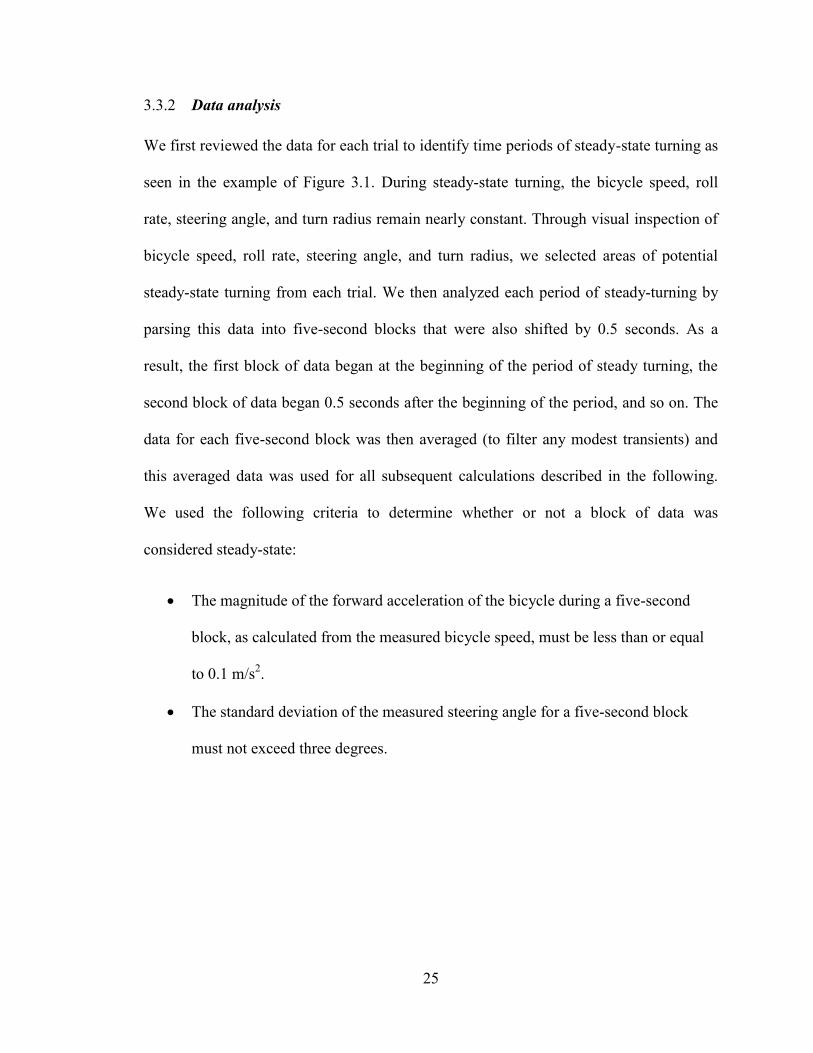
25
Data analysis 3.3.2
We first reviewed the data for each trial to identify time periods of steady-state turning as
seen in the example of Figure 3.1. During steady-state turning, the bicycle speed, roll
rate, steering angle, and turn radius remain nearly constant. Through visual inspection of
bicycle speed, roll rate, steering angle, and turn radius, we selected areas of potential
steady-state turning from each trial. We then analyzed each period of steady-turning by
parsing this data into five-second blocks that were also shifted by 0.5 seconds. As a
result, the first block of data began at the beginning of the period of steady turning, the
second block of data began 0.5 seconds after the beginning of the period, and so on. The
data for each five-second block was then averaged (to filter any modest transients) and
this averaged data was used for all subsequent calculations described in the following.
We used the following criteria to determine whether or not a block of data was
considered steady-state:
The magnitude of the forward acceleration of the bicycle during a five-second
block, as calculated from the measured bicycle speed, must be less than or equal
to 0.1 m/s2.
The standard deviation of the measured steering angle for a five-second block
must not exceed three degrees.

26
Figure 3.1. Identification of a region of steady-state turning. Bicycle speed, roll rate, steering angle, and
instantaneous turn radius were used to identify a region of steady-state turning for processing. The region
of steady turning for the example trial shown (a medium speed, clockwise turn with a turn radius of 9.14
meters) lies within the two vertical (black) lines. Another large region of steady-state turning begins around
90 seconds and ends at approximately 125 seconds. The turn radius data has been truncated to highlight the
steady-state turning region of interest.
The inertial measurement unit defines a sensor frame of reference ( ) which
differs from the bicycle-fixed frame ( ) illustrated in Figure 3.2A. The orientation
of the sensor frame of reference relative to the conventional vehicle dynamics axes [94]
for a bicycle is illustrated in Figure 3.2C. The acceleration and angular velocity
components measured in the sensor-fixed frame ( and ) must be transformed
into components measured in the bicycle-fixed frame ( and ) for subsequent data
reduction. This is achieved using, for example,

27
[
] (3.1)
where denotes the seat tube angle relative to vertical. For the instrumented bicycle used
in this study, degrees.
The average radius of the turn for each five-second block was then determined from
√(( ) ( ) )
(3.2)
where denotes the corresponding bicycle speed and and denote the angular
velocities about the axes defined by and illustrated in Figure 3.2B. The angular
velocities and were determined using the outputs from the three sampled single-
axis angular rate gyros. Note that upon assuming the pitch rate of the bicycle is
negligible, the denominator of (3.2) represents the yaw rate; in a steady turn, the angular
velocity is vertical (i.e., the component is zero).

28
Figure 3.2. (A) The rotation of the bicycle-fixed frame )ˆ,ˆ,ˆ( kji eee relative to the sensor-fixed frame
)ˆ,ˆ,ˆ( 321 eee . (B) The rotation of the bicycle-fixed frame relative to the inertial frame )ˆ,ˆ,ˆ( ZYX eee . (C) A
sketch of a bicycle showing the relationship of the sensor-fixed frame )ˆ,ˆ,ˆ( 321 eee to the conventional
vehicle dynamics coordinate system ),,( ZYX when the bicycle is in the upright position. Note that
)ˆ,ˆ,ˆ( ZYX eee is aligned with ),,( ZYX .
The bicycle roll angle ( ), which we define as the roll angle of the rear of the bicycle
frame relative to vertical as in [2], follows from the measured bicycle-fixed frame
acceleration, by exploiting the fact that the accelerometer functions as an
inclinometer during steady-state turning. In particular, the IMU measures the acceleration
at the location of the sensor plus the acceleration of gravity. Therefore, includes the
centripetal acceleration for steady turning (directed in the horizontal plane) and the
acceleration due to gravity (directed along the vertical):
(3.3)
where is the forward bicycle speed and is the turn radius; positive values of
correspond to clockwise turns whereas negative values correspond to counter-clockwise
turns. The frame ( ) is related to the frame ( ) through:

29
[
] [
] [
] (3.4)
Substituting (3.4) into (3.3) and solving for the bicycle roll angle ( ) yields:
(
) (
) (3.5)
where and are the (average) values of the measured acceleration along the and
axes in Figure 3.2. The results (3.3) and (3.5) also assume that the distance between the
accelerometer and the center of mass of the bicycle/rider system is negligible compared
to the radius of the turn and that the bicycle-fixed axis defined by is the heading
direction.
We confirmed the accuracy of the above technique to estimate the bicycle roll angle by
comparing the roll angle estimated from (3.5) to independently measured simulated roll
angles. We created simulated roll angles by installing the IMU on a jig fastened to a two-
wheeled bicycle trailer (Figure 3.3) that allows us to set and measure the simulated roll
angle of the IMU using a high-precision inclinometer (resolves the pre-set roll angles to
within 0.01 degrees). Assuming that the roll of the trailer remains negligible, the
simulated roll angle of the inertial measurement unit remains constant at a pre-set and
measured value when the bicycle pulls the trailer around a constant radius turn on level
pavement. We conducted 20 trials, in which we varied the turn radius (9.14, 27.73, and
32.31 meters), the bicycle speed (slow, medium, and fast), and the jig roll angle (-17.34,
11.49, 1.63, and -30.51 degrees). The difference between the estimated roll angle and the

30
independently measured simulated roll angle was 1.10 ± 0.78 degrees (mean ± standard
deviation) confirming that the acceleration-based measurement technique successfully
estimates the roll angle during steady-state turning.
Figure 3.3. A jig was used to validate our method of estimating the bicycle roll angle by allowing us to
orient the inertial measurement (IMU) at a fixed simulated roll angle. The simulated roll angle was
independently measured using an inclinometer that can resolve the roll angle to within 0.01 degrees
(inset photograph). The jig was secured to a bicycle trailer and pulled behind the instrumented bicycle on
level pavement. The white rectangle indicates the location of the IMU on the jig secured to the trailer.
Theoretically, the bicycle roll angle could also be estimated by using the measured
angular velocities:
(
) (3.6)
However, this method yields poor estimates for roll angles less than four degrees due to
the limited resolution of the rate gyros. The estimate provided by (3.5) does not suffer
from this limitation and yields superior estimates.

31
Due to the placement of the steering angle optical encoder relative to the steering torque
sensor, the angular displacement of the handlebar and stem about the steering axis
( ) was recorded instead of the angular displacement of the front wheel about
the steering axis ( ). However, these values differ by a small but measurable twist of
the assembly. The true steering angle, or angular displacement of the front wheel about
the steering axis, is given by
(3.7)
where is the measured steer torque and 4.97 Nm/deg is the aforementioned stiffness of
the torque sensor assembly. For all our analyses and figures we use per (3.7).
For statistical analysis and for plotting, we averaged the results from the five-second
blocks for each trial (one combination of subject, lean condition, speed and radius),
which yields one set of values per trial. The total number of trials used for analysis is 134
instead of the total measured (2 x 81 = 162) because data for 28 trials failed the
aforementioned criteria for steady-state.
Theoretical model for steady-state turning 3.3.3
We employ the Whipple bicycle model [3] as presented by Meijaard et al. [2] to derive a
model for steady-state turning similar to that for a vehicle [95-97]. The Whipple bicycle
model consists of four rigid bodies: a rear wheel, a rear frame with a rider rigidly
attached to it, a front frame consisting of the front handlebar and fork assembly, and a
front wheel. The model assumes that all bodies are laterally (left-right) symmetric and
that the wheels have circular symmetry. Motion of the rider relative to the frame,
32
structural compliance and damping, joint friction, and tire compliance and slip are
neglected. The tire contacts with the ground are modeled as knife-edge rolling point-
contacts. The model is configured with seven generalized coordinates: the location of the
rear-wheel contact with the ground ( ), the rotation of the front and rear wheels
( ), the yaw rotation ( ), the roll or lean angle ( ) of the bicycle frame, and the
steering angle ( ). As noted in [2], only three of the generalized coordinates are
independent upon accounting for four non-holonomic rolling constraints. After
linearizing the model about upright, straight-line motion and treating forward speed as a
parameter, only two independent generalized coordinates remain: steer ( ) and lean or
roll ( ).
The resulting linearized equations of motion, as presented in [2] (Equation 5.3 therein),
are:
[ ] (3.8)
where [ ] are the remaining generalized coordinates for the roll (lean) and steer
angles and [ ] are the associated generalized forces representing the lean and
steer torques. The first and the second equation of (3.8) are referred to as the lean
equation and the steer equation, respectively [2]. The other quantities appearing in (3.8)
include the forward speed , gravity , and the matrices and as defined in
Appendix A of [2].
During a steady turn, the steering angle ( ) and the lean or roll angle ( ) remain constant,
reducing (3.8) to the equilibrium equation

33
[ ] (3.9)
Assuming that the lean torque in a steady-state turn vanishes ( ), the lean and steer
equations become
( ) (3.10)
( ) (3.11)
where and are constants defined by Equations (A.14)-
(A.19) in Appendix A. Note that Equation (3.11) yields the steering torque ( ) in terms
of the bicycle configuration ( ) and forward speed . Under the same conditions, the
yaw rate ( ) given by Equation B6 in [2] reduces to
(3.12)
where is the steer axis tilt, is the bicycle wheel base, and is the radius of the steady
turn. (Note that and are positive for clockwise turns and negative for counter-
clockwise turns and that is measured from the center of the turn to the rear wheel
ground contact point.) The required steer angle is therefore
(3.13)
and substitution of this result into (3.10) yields the required lean angle

34
( )
( ) (3.14)
Finally, substitution of (3.13) and (3.14) into (3.11) yields the required steering torque
( (
) ( ))
( ) (3.15)
Comparison of the model to experimental data 3.3.4
In the following, we compare the measured roll angle, steer angle and steer torque to
those predicted by the model above. In particular, we use the measured bicycle speed ( )
and nominal turn radius ( ) in the following sequence of calculations.
(1) The bicycle roll angle ( ), or roll of the bicycle frame, is calculated using
Equation (3.14).
(2) The steer angle ( ) is calculated using Equation (3.13).
(3) The steering torque ( ) is calculated using Equation (3.15).
We also compute the steering torque/steer angle ratio and the roll angle/steer angle ratio.
The calculations require knowledge of the bicycle parameters described in Appendix A
and summarized in Table A.2 for both subjects.
The statistical fit of the experimental data to the model predictions is determined by
calculating the correlation coefficient between the experimental and theoretical results
and the linear least squares fit of the experimental to theoretical results. Where the model

35
predicts linear relationships, we compared the linear least squares fits of the experimental
data to the linear relationships predicted by the model. We used t-tests with an alpha level
of 0.05 to determine statistical significance.
3.4 Results
Roll angle. The estimated bicycle roll angle, calculated from Equation (3.5), is plotted
versus normalized lateral acceleration in Figure 3.4 together with the roll angle predicted
by the model, calculated from Equation (3.14). Due to the fact that the magnitude of
is only about 2.5% of the magnitude of , the model predicted roll angle is nearly
linear in lateral acceleration, as shown in Figure 3.4. The non-linear effects for the
experimental conditions are contained within the width of the plotted line. The model
predicts 99.8% of the variation of the measured bicycle roll angle for the normal riding
trials, i.e. trials without exaggerated rider lean relative to the bicycle frame. Moreover,
the model predicts 95.6% of the variation of the estimated bicycle roll angle, regardless
of rider posture (normal riding or leaning body into or out of the turn relative to the
bicycle frame). The linear fit of measured versus predicted bicycle roll angle for all lean
conditions has a slope that is not statistically significantly different from 1.0 (Table 3.2),
which further confirms that this model closely predicts the measured lean angle.
A rider leaning into or out of a turn relative to the bicycle frame can significantly alter the
slope of the linear fit by approximately ±13%. This arises from the additional roll of the
bicycle caused by the lateral offset of the center of mass of the bicycle/rider system. For
example, a rider leaning into a clockwise turn will cause the bicycle roll angle to
decrease, resulting in a bicycle roll angle slightly less than that predicted by the model.
36
Both subjects clearly exhibit this trend, as shown by the dark gray ‘ ’ symbols in Figure
3.4. The opposite trend arises for a rider leaning out of a clockwise turn, as shown by the
light gray ‘ ’ symbols in Figure 3.4. If we assume that the estimated bicycle roll angle is
accurate, we can then also estimate the additional roll of the bicycle caused by a lateral
shift in the center of mass as the difference between the estimated and the model
predicted roll angles. The mean values for the estimated additional roll are reported in
Table 3.1. Both riders were able to create significant additional roll of the bicycle by
leaning; on average, the estimated additional roll angle of the bicycle was -2.5 degrees
and 2.0 degrees when the riders leaned into and out of the turn, respectively. During
normal riding, riders tended to lean slightly into the turn relative to the bicycle frame,
generating an estimated additional roll angle of -0.2 degrees. The very small deviations
between the normal riding data and the model could derive from small lateral shifts in the
center of mass, asymmetric stance on the bicycle, errors in the estimated bicycle roll
angle (see Section 3.3.2), and transient as opposed to steady-state conditions.

37
Figure 3.4. Bicycle roll angle versus normalized lateral acceleration. The experimental data are predicted
well by the model (slope = 1.00, R2 = 0.956). Deviation from the model prediction can be interpreted as
additional roll of the bicycle caused by a lateral shift in the bicycle/rider system center of mass. Positive
values of lateral acceleration correspond to clockwise turns; negative values correspond to counter-
clockwise turns. Note that the model predicted bicycle roll angle is nearly linear in lateral acceleration; the
non-linear effects for the experimental conditions are contained within the width of the plotted line.
Table 3.1. Differences between the estimated bicycle roll angle and the model predicted roll angle for
different lean conditions. A positive value indicates that a rider can increase the magnitude of the bicycle
roll angle by leaning, whereas a negative value indicates that rider can decrease the magnitude.
Subject normal riding leaning body into turn leaning body out of turn
1 -0.4° -1.7° * 1.0° *
2 -0.1° -3.1° * 2.7° *
1 & 2 -0.2° -2.5° * 2.0° *
Note: * indicates that the mean value is significantly different than the ‘normal riding’ lean condition ( =
0.05).
Steering angle. The measured steering angle ( ) shown in Figure 3.5 is also predicted
well by the model, as evidenced by the linear fit and R2 values reported in Table 3.2. The
model predicts 99.5% of the variation in the measured steering angle for all lean
conditions. Linear fits to the measured steering angle for specific lean conditions were
not significantly different than the fit to all trials. However, all linear fits had slopes
significantly less than 1.0, indicating that the model slightly over-predicts the measured
steering angle. Measured steady turning steering angles ranged in magnitude from
approximately zero to 7.5 degrees. Some deviations of the experimental data from the

38
model can likely be attributed to the transient dynamics that arise when the human rider
makes steering corrections to remain upright and to follow the desired path. For example,
the data point located far below the model prediction (predicted steering angle 7
degrees, measured steering angle 5 degrees) is from a trial where the subject was
required to ride around the smallest radius curve at the slowest speed while leaning his or
her body into the turn, which was the most challenging riding condition. While the data
from this trial formally met our criteria for steady-state (see Section 3.3.2), closer
inspection of the trial revealed that the subject used small steering angles for the majority
of the trial and used occasional larger steering corrections to stay on the prescribed path.
Table 3.2. Summary of the linear fit )( bmxy of measured values to model predicted values.
Lean
condition
Predictor, from
model ( ) Predicted variable ( ) Slope ( ) y-intercept ( ) R
2
all bicycle roll angle estimated bicycle roll angle 1.00 † 0.56° 0.956
normal bicycle roll angle estimated bicycle roll angle 0.99 † 0.47° * 0.998
rider lean
into turn bicycle roll angle estimated bicycle roll angle †* 0.87 †* 1.45° 0.968
rider lean
out of turn bicycle roll angle estimated bicycle roll angle †* 1.14 * -0.11° 0.971
all steering angle measured steering angle † 0.96 † -0.28° 0.995
normal steering angle measured steering angle † 0.97 † -0.26° 0.995
rider lean
into turn steering angle measured steering angle † 0.94 † -0.26° 0.994
rider lean
out of turn steering angle measured steering angle † 0.98 † -0.32° 0.998
all steering torque measured steering torque 1.04 -0.07 Nm 0.065
normal steering torque measured steering torque 0.86 † -0.07 Nm * 0.566
rider lean
into turn steering torque measured steering torque †* -1.33 †* -0.68 Nm 0.155
rider lean
out of turn steering torque measured steering torque †* 3.98 †* 0.54 Nm * 0.634
Note: All reported slopes ( ) are significantly different than zero and all values of R2 are significant
( ).
* indicates that a value is significantly different than the value for the corresponding ‘all’ lean condition.
† indicates that a linear fit constant is significantly different from a fit to the model (m = 1.0, b = 0.0).

39
Figure 3.5. Measured steering angle versus model predicted steering angle. The experimental data are
predicted well by the model (slope = 0.96, R2 = 0.995). The clusters of data correspond to the different radii
of turns tested experimentally. Scanning from left to right, the data groups correspond to: counter clockwise
turning around radii of approximately 12.2, 18.3, 28.0 and 32.5 meters and clockwise turning around turns
of 22.9 and 9.1 meters.
Steering torque. The steering torque for all lean conditions is not predicted well by the
model, as shown in Figure 3.6. However, the model does provide a reasonable fit to the
normal riding case, as evidenced by the linear fit and R2 values reported in Table 3.2. For
normal riding, the slope of the linear fit is not significantly different from 1.0, indicating
that the measured steering torque is not significantly different from the model
predictions. However, the model is only able to account for 56.6% of the variation in the
experimental data. For the rider-lean conditions, the model is not as useful for predicting
the steering torque. For the rider leaning into the turn relative to the bicycle frame, the
model predicts steering torques that are in the opposite direction with magnitudes
approximately 33% less than the measured steering torque. For the rider leaning out of
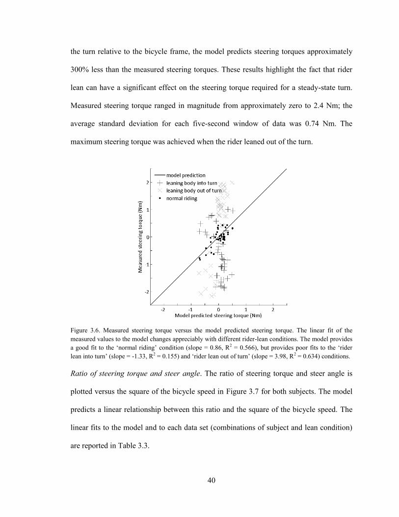
40
the turn relative to the bicycle frame, the model predicts steering torques approximately
300% less than the measured steering torques. These results highlight the fact that rider
lean can have a significant effect on the steering torque required for a steady-state turn.
Measured steering torque ranged in magnitude from approximately zero to 2.4 Nm; the
average standard deviation for each five-second window of data was 0.74 Nm. The
maximum steering torque was achieved when the rider leaned out of the turn.
Figure 3.6. Measured steering torque versus the model predicted steering torque. The linear fit of the
measured values to the model changes appreciably with different rider-lean conditions. The model provides
a good fit to the ‘normal riding’ condition (slope = 0.86, R2 = 0.566), but provides poor fits to the ‘rider
lean into turn’ (slope = -1.33, R2 = 0.155) and ‘rider lean out of turn’ (slope = 3.98, R
2 = 0.634) conditions.
Ratio of steering torque and steer angle. The ratio of steering torque and steer angle is
plotted versus the square of the bicycle speed in Figure 3.7 for both subjects. The model
predicts a linear relationship between this ratio and the square of the bicycle speed. The
linear fits to the model and to each data set (combinations of subject and lean condition)
are reported in Table 3.3.

41
For both subjects, the model predicts a positive slope of approximately 0.1 kg/radian. The
linear fits to the data for Subject 1 all have negative slopes; however, only the slope of
the fit to the ‘normal’ lean condition is significantly different from the model and
significantly different from zero. By contrast, the linear fits to the data for Subject 2 all
have positive slopes; none of the slopes are significantly different from the model or
significantly different from zero. For both subjects, the model predicts a y-intercept of
approximately -5.9 Nm. Both subjects were able to significantly change the y-intercept
by leaning their bodies into or out of a turn relative to the bicycle frame. A rider leaning
his/her body into a turn causes a positive steering torque/steering angle ratio, requiring a
rider to apply steering torque in the same direction as the steering angle. A rider leaning
his/her body out of a turn causes a negative steering torque/steering angle ratio, requiring
a rider to apply steering torque in the opposite direction from the steering angle. Only one
of the R2 values for the linear fits is significantly different from zero (Subject 1, normal
lean condition), which is expected from slope values not significantly different from zero.
A linear model adequately predicts the data for the normal lean condition, as evidenced
by the sum of squared errors (SSE) in Table 3.3.

42
Table 3.3. Summary of the linear fit bvmT )()/( 2 .
Subject Lean condition Slope (m) y-intercept (b) R2 SSE
model (subject 1) -- 0.097 kg -5.986 Nm 1 0 (Nm)2
subject 1 all -0.070 kg -0.250 Nm * 0.008 18508 (Nm)2
subject 1 normal †* -0.088 kg * -0.374 Nm †* 0.202 367 (Nm)2
subject 1 rider lean into turn -0.058 kg †* 16.490 Nm * 0.007 4518 (Nm)2
subject 1 rider lean out of turn -0.051 kg †* -17.238 Nm * 0.012 1794 (Nm)2
model (subject 2) -- 0.100 kg -5.868 Nm 1 0 (Nm)2
subject 2 all 0.142 kg -7.708 Nm * 0.015 61924 (Nm)2
subject 2 normal 0.159 kg † -9.781 Nm * 0.127 2988 (Nm)2
subject 2 rider lean into turn 0.117 kg †* 26.432 Nm * 0.027 7786 (Nm)2
subject 2 rider lean out of turn 0.127 kg †* -36.509 Nm * 0.047 4060 (Nm)2
Note: For the linear fits to experimental data,
* indicates that a value (m, b, or R2) is significantly different than the model
† indicates that a value is significantly different from zero.
Figure 3.7. The ratio of steering torque to steer angle versus bicycle speed squared. A negative ratio means
that a rider must apply a counter-clockwise (negative) steering torque when applying a clockwise (positive)
steer angle, whereas a positive ratio means that a rider must apply a clockwise (positive) steering torque
when applying a clockwise (positive) steer angle. Both riders were able to significantly change the ratio by
leaning into or out of a turn.
Ratio of roll angle and steer angle. The ratio of the roll angle and steer angle is plotted
versus the square of the bicycle speed in Figure 3.8 for both subjects. The model predicts
a linear relationship between this ratio and the square of the bicycle speed. The linear fits
to the model and to each data set (combinations of subject and lean condition) are
reported in Table 3.4.

43
For both subjects, the model predicts a positive slope of approximately 0.1 s2/m
2. Almost
all of the linear fit slopes for Subject 2 are significantly different than the model, whereas
only one of the linear fit slopes (rider lean out of turn) for Subject 1 is significantly
different than the model. However, all of the slopes are positive, which indicates that the
ratio of roll angle/steer angle increases with increasing speed. For both subjects, the
model predicts a y-intercept of approximately -0.02. Both subjects were able to
significantly change the y-intercept by leaning their bodies into or out of a turn relative to
the bicycle frame. A rider leaning his/her body into a turn reduces the roll angle/steer
angle ratio, whereas a rider leaning his/her body out of a turn increases the roll
angle/steer angle ratio. For most trials and speeds, the ratio of roll angle/steer angle is
positive, indicating that in a steady turn a rider must lean the bicycle in the same direction
that he/she is steering. However, at low speeds and when a rider leans out of a turn, the
ratio can be negative indicating that a rider must actually lean the bicycle in the opposite
direction that he/she is steering. A linear model adequately predicts the data for all lean
conditions, as evidenced by the R2 values and sum of squared errors (SSE) in Table 3.4.
Table 3.4. Summary of the linear fit bvm )()/( 2 .
Subject Lean condition Slope (m) y-intercept (b) R2 SSE
model (subject 1) -- 0.092 s2/m
2 -0.024 1 0
subject 1 all † 0.085 s2/m
2 -0.115 †* 0.895 25.3
subject 1 normal † 0.090 s2/m
2 -0.164 †* 0.975 2.5
subject 1 rider lean into turn † 0.080 s2/m
2 †* -0.568 †* 0.894 7.3
subject 1 rider lean out of turn †* 0.085 s2/m
2 †* 0.429 †* 0.972 1.6
model (subject 2) -- 0.092 s2/m
2 -0.021 1 0
subject 2 all †* 0.080 s2/m
2 0.103 †* 0.816 66.3
subject 2 normal †* 0.085 s2/m
2 -0.007 †* 0.987 1.7
subject 2 rider lean into turn † 0.082 s2/m
2 †* -0.977 †* 0.886 13.7
subject 2 rider lean out of turn †* 0.072 s2/m
2 †* 1.263 †* 0.926 5.2
Note: For the linear fits to experimental data,
* indicates that a value (m, b, or R2) is significantly different than the model
† indicates that a value is significantly different from zero.

44
Figure 3.8. The ratio of bicycle roll angle and steering angle versus bicycle speed squared. Both subjects
were able to significantly change the y-intercept of a linear fit to the data by leaning into or out of a turn.
3.5 Discussion
As illustrated in Figure 3.4, the estimated roll angle of the bicycle is predicted well by the
steady-state turning model developed in Section 3.3.3. For a motorcycle in steady
turning, Fu [90] showed that the roll angle is predicted best when the model includes the
gyroscopic effects of the motorcycle wheels and engine, as well as tires with a circular
cross-section, a conclusion also supported by Prem [45]. In contrast, we find that for a
bicycle, the roll angle is predicted rather well upon considering the wheel as a thin disk
with a zero-radius edge.
The above results also demonstrate that a seated rider can generate significant additional
roll of a bicycle (Table 3.1) simply by leaning his/her upper body into or out of a turn
relative to the bicycle frame. In fact, lean dynamics arise even while riding in a straight
line as observed by riders maintaining position on a treadmill [93]. In practice, cyclists
often lean their bodies into a turn relative to the bicycle frame to increase pedal clearance,
such as a road cyclist racing in a criterium. As illustrated in Figure 3.4, by leaning into

45
the turn, the cyclist decreases the roll angle of the bicycle, and therefore gains pedal
clearance. Alternatively, cyclists may lean their bodies out of a turn relative to the bicycle
frame, as in the case a mountain biker leaning to avoid trees or branches lining the trail.
As illustrated in Figure 3.4, by leaning out of the turn, the cyclist increases the roll of the
bicycle but decreases the lateral distance of her/his body from the base of support of the
bicycle.
The steer angle of the bicycle is predicted well by the model (Table 3.2 and Figure 3.5).
The linear fit of the data to the model results yields values of the slope slightly less than
one (Table 3.2), indicating that the model slightly over-predicts the steer angle. Similar to
these results, Fu [90] and Prem [45] observed that for a motorcycle in a steady-turn, the
steering angle is over-estimated by steady-state turning models. The y-intercept of the
linear fit is approximately -0.3 degrees, regardless of rider lean, indicating that perhaps
the method of zeroing the steering angle encoder introduced a slight systematic error.
The steady-state turning model reasonably predicts the steering torque of a bicycle when
there is no exaggerated rider lean relative to the bicycle frame. The model explains 56.6%
of the variation in the measured data for the normal riding condition and the slope of the
linear fit to the data is not significantly different from 1.0. The discrepancies between the
model and experimental data for the normal riding condition might arise from the
measurement limitations of the current torque sensor. In particular, all measured steering
torques were less than 10% of the full scale range of the sensor, rendering the torque
measurements sensitive to both small systematic and random error sources. The steering
torque required to steer a bicycle around a steady curve is substantially smaller than that
for a motorcycle; we measured a maximum steering torque of 2.4 Nm for the tested

46
conditions, whereas Prem [45] and Bortoluzzi et al. [98] measured steering torques up to
approximately 10 Nm for a motorcycle with a non-leaning rider. In addition, the steering
torque during each five second window varied significantly, with an average standard
deviation of 0.74 Nm. Another source of error could derive from the fact that the model
predicted steering torque calculation is sensitive to the configuration of the bicycle;
deviations of the measured steer angle and estimated bicycle roll angle from model
predictions translate to errors in the predicted steering torque. Another possibility is that
any inaccuracies in the parameters used to calculate the model predicted steering torque
for the instrumented bicycle will have a larger effect on the fit when the range of steering
torque is small, such as in the normal riding condition. For example: when a subject
changes his/her position on the bicycle, the bicycle/rider center of mass location ( )
changes, which alters the magnitude of the steering torque required by the rider. In
addition to measurement errors, discrepancies between the data and the model could also
arise from simplifications in the model. In particular, the accuracy of the model could
likely be improved by allowing tires with circular cross sections, large roll angles, large
steer angles, and more realistic tire parameters (particularly pneumatic trail) [6, 79, 87,
92]. The model also does not account for torque that could arise from other factors, such
as the effects of the cable housing and transient dynamics.
The accuracy of the steering torque predicted by the model varies significantly depending
on the rider-lean condition (Table 3.2). The model does not account for rider lean relative
to the bicycle frame, which can significantly change the roll angle of the bicycle. The
experimental results demonstrate that a rider can significantly change the steering torque
required to negotiate a steady-turn by simply leaning into or out of the turn. Leaning into

47
the turn can produce a dramatic effect, namely the complete reversal of the required
steering torque. If the roll of the bicycle is changed by a leaning rider, the first term of
Equation (3.11) is affected, which can reverse the sign of the steering torque. Several
models have been derived to explore how a rider is able to ride a bicycle with no-hands,
i.e., ride with zero steering torque [5-7, 88]. These models incorporate the lean (reaction)
torque that is applied between the rider’s upper body and the bicycle. While lean torque is
not measured herein, the results clearly demonstrate that upper body lean can control the
sign and magnitude of the steering torque required to negotiate a steady-turn. Therefore,
it is also possible for a rider to adjust his/her body lean to achieve zero steering torque,
thereby enabling no-handed riding. Similarly, for “hands-on” riding, a rider may adjust
his/her lean to control the steering torque. The discrepancies between the model and
measured steering torque highlight that a rider can significantly alter the required steering
torque by simply adjusting his or her lateral position on the bicycle.
The ratio of the steering torque to the steering angle is similar to the acceleration index
employed in the motorcycle handling literature as a measure of maneuverability [79, 92,
99]. The steering torque/steering angle ratio represents ‘steering stiffness,’ which has
been identified as a useful parameter for designing bicycles [100]. However, as noted by
Prem [45], steady-state response parameters (including the acceleration index and
steering stiffness) can vary substantially among different motorcycles with ‘acceptable’
handling characteristics. The acceleration index indicates the direction of the steering
torque relative to the direction of the steady turn [91]. Similarly, the sign of the steering
torque/steering angle ratio indicates whether steering torque must be applied in the same
direction as the steer angle (usually into the turn) or in the opposite direction (usually out

48
of the turn). Similar to the steady turning of a motorcycle [92, 98], we find that the lateral
displacement of a rider’s center of mass (rider lean) relative to the bicycle frame has a
significant effect on the direction of the required steering torque.
The above discussion suggests that the steering torque is not an easy quantity for a rider
to predict or interpret, a conclusion also supported by Prem [45] and Watanabe and Segel
[101] who noted that measured steering torque does not provide useful feedback to a
motorcycle rider. For instance, a rider can simply change the required control strategy
from applying a steer torque out of the turn to applying a steer torque into a turn by
leaning into the turn. In addition, a dynamically leaning bicycle rider constantly changes
the required steering torque when pedaling and shifting weight from side-to-side. A more
predicable or useful cue is suggested by the steer angle results, which are insensitive to
even exaggerated rider lean during steady-state turning.
3.6 Summary and Conclusions
Steady-state turning arises when the bicycle/rider negotiates a constant radius turn at
constant speed and roll angle. This chapter examines steady-state turning using a bicycle
instrumented to measure steering torque, steering angle, bicycle speed, bicycle
acceleration, and bicycle angular velocity. We report data obtained from 134 trials using
two subjects executing steady turns defined by nine different radii, three speeds (slow,
medium, fast), and three rider lean conditions relative to the bicycle frame (normal,
leaning into the turn, leaning out of the turn). We also introduce a model for the steady-
state turning of the bicycle/rider system and compare the experimental data to the model
predictions for the bicycle roll angle, steering angle, steering torque, steering torque/steer
angle ratio, and roll angle/steer angle ratio.

49
The model explains 95.6% of the variability in the measured bicycle roll angle for all lean
conditions, 99.5% of the variability in the measured steering angle for all lean conditions,
and 56.6% of the variability in the measured steering torque for the normal riding lean
condition. The experimental data demonstrate that rider lean (lateral shifting of the
bicycle/rider center of mass relative to the bicycle frame) strongly influences the steering
torque, suggesting that rider lean plays an important role in the control of a bicycle. By
contrast, the steering angle is largely insensitive to rider lean, suggesting that using the
steering angle as a cue for bicycle control is advantageous over using steering torque.

50
CHAPTER 4: QUANTIFYING THE PROCESS OF LEARNING TO RIDE A BICYCLE USING
MEASURED BICYCLE KINEMATICS
4.1 Chapter summary
Currently, it is difficult to determine when a novice bicycle rider is ready to ride without
training wheels or external assistance. It is also unclear what must be learned by a rider in
order for him/her to be successful riding a bicycle. In this study, we quantify the changes
that occurred as 15 children with disabilities learned to ride bicycles during a specialized
bicycle training camp. These changes are revealed by three inertial measurement units
(IMUs) used to measure bicycle kinematics. Out of 15 subjects, 11 were successful in
riding a bicycle without assistance by the end of the camp. The peak value of the cross-
correlation between steer and roll angular velocities was significantly greater for riders
who ultimately succeeded in riding a bicycle without assistance. This finding suggests
that rider learning can be quantified by increased correlation between bicycle steer rate
and roll rate. In essence, learning to steer in the direction of lean is an essential skill in
learning to ride a bicycle.
4.2 Introduction
Riding a bicycle is a skill that many people learn quite easily as reflected in the common
assertion, “it’s as easy as riding a bike.” However, there is little scientific understanding
about how we learn to ride and balance a bicycle. What does a new rider learn when s/he
finally is able to balance on a bicycle? When is s/he ready to ride without assistance?
51
What underlying skills define the learning process? These questions may seem
unimportant to those who have quickly learned to ride, but to those who have not
succeeded in learning to ride or to those struggling to help others learn to ride, these
questions remain perplexing.
Learning to ride a bicycle has many benefits, especially for populations possessing
learning disabilities. For example, learning to ride increases the physical activity of
children with Down syndrome [46]. Also, being able to ride a bicycle can provide those
who cannot drive a car due to their disabilities with a means of efficient transportation.
Understanding rider learning could improve programs that teach affected populations to
ride and could also promote bicycle designs and assistive technologies that aid the
learning process or help humans maintain stability when riding.
By analogy, to balance during standing or walking, a person must position their mass
center above their center of pressure [47, 76]. Doing so requires significant coordination
of body movements, especially in challenging balancing tasks [48]. Researchers have
quantified this coordination to understand the development of mature gait [102] and to
detect differences in balance performance [49, 54, 57, 68]. Unfortunately, this
understanding has not yet translated to balancing a bicycle, which further requires
coordination of body movements with bicycle movements.
This additional coordination of bicycle and body movements is often learned with the
assistance of others and/or with training aids. However, it remains unclear what
assistance works best or when a learner is ready to advance to a bicycle without training
aids. Typical training aids include training wheels and balance bikes. Training wheels

52
significantly increase the base of support when a bicycle begins to tip. The same effect
arises on pedal-less balance bikes on which a learner uses his/her feet to propel the
bicycle forward. Additionally, a balance bike rider’s feet can also readily stabilize the
bike during incipient tipping. A relatively new training aid [103] uses a gyroscope
mounted in the front wheel to augment stability. While any of these training aids can
ultimately help riders learn to ride, it remains unclear what underlying skill (or set of
skills) defines this learning process.
The task of human/bicycle balance is complex and not well understood. While recent
studies expose the self-stability of bicycles alone [2], other studies demonstrate that
humans can readily balance bicycles that lack self-stability [16, 17]. In addition, a
number of proposed control systems successfully stabilize bicycle models [5, 7, 19, 30],
yet they do not model or expose the human learning process. Despite our lack of
understanding of this learning process, the basic strategy to keep a bicycle upright,
namely steering into the lean, is well known. Schwab et al. [7] demonstrate that a simple
steer-into-the-lean intuitive controller is capable of stabilizing a bicycle. Likewise, a
patented training method [104] reinforces this skill. Kooijman et al. [11] further explain
that the aforementioned self-stability of a bicycle results from its reaction to steer into the
lean. Clearly, balancing a bicycle requires a specific relationship between steer and lean
dynamics.
Doyle [16] demonstrated this relationship by measuring the cross-correlation of bicycle
steer and lean (also referred to as roll) responses. In particular, the steer angle was highly
correlated to the roll angle at some time shift or lag. Similar to the findings of Doyle are
the findings of van Lunteren and Stassen [105] who utilized a bicycle simulator to study

53
human/bicycle dynamics. Their results confirm that the steer angle lags and is highly
correlated to the roll angle. A human riding a bicycle represents a closed-loop system in
which the rider employs sensory feedback to achieve stabilization of the bicycle/rider
system. Because successful bicycle riding requires a well-defined relationship of steer
and roll dynamics, we hypothesize that this relationship must also develop as a novice
rider successfully learns to ride.
The objective of this study is to quantify how human subjects learn to ride a bicycle by
tracking key kinematic changes in bicycle roll and steer dynamics during the learning
process. The subjects for this study are children who participated in a specialized bicycle
training camp called Lose the Training Wheels; refer to www.losethetrainingwheels.org.
Children enter this camp having no ability to ride a bicycle and either acquire that ability
or make significant progress towards that goal by the end of the week-long camp [46,
106]. Therefore, this camp provides an ideal setting for tracking the changes that arise as
a child transitions from a non-rider to a rider. A previous analysis of pilot data [107]
helped develop our hypotheses and methods. We hypothesize that the measured bicycle
steer and roll angular velocities will become significantly correlated as a successful
subject progresses through training. In addition, we hypothesize that the average bicycle
speed, the standard deviation of the roll angular velocity, and the standard deviation of
the steer angular velocity will all increase with training. We open the Methods section by
summarizing the training protocol, instrumentation, experimental protocol, and data
analysis methods. In the Results and Discussion section, we quantify the salient changes
in the measured kinematical variables that emerge as subjects successfully learn to ride.

54
4.3 Methods
We measured the steer and roll dynamics bicycles ridden by 15 participants as they
progressed through a bicycle training camp organized by the organization Lose the
Training Wheels. The camp provides five consecutive days (Monday-Friday) of
individual instruction for 75 minutes per day for each participant. The children (ages 8-19
years) in the camp had a range of disabilities, which included primary diagnoses of Down
syndrome (n = 3), Autism Spectrum Disorder (n = 10), cerebral palsy (n = 1), and
attention deficit hyperactivity disorder (n = 1); Table 4.1 reports subject details. None of
the participants were able to ride/balance a bicycle prior to entering the camp. Our goal
was to reveal the underlying changes in bicycle steer and roll dynamics as each
participant learned to balance a bicycle, regardless of disability. The experimental
protocol was approved by the University of Michigan Institutional Review Board and this
included written informed consent from parents/guardians and assent from the
participating subjects.

55
Table 4.1. Subject details.
Subject Age (years) Learned to ride? Primary Diagnosis
A 19 yes Down syndrome
B 15 yes autism spectrum disorder
C 12 yes autism spectrum disorder
D 14 yes autism spectrum disorder
E 9 yes autism spectrum disorder
F 8 no Down Syndrome
G 18 yes autism spectrum disorder
H 10 no Down Syndrome
I 15 no cerebral palsy
J 16 no attention deficit hyperactivity disorder
K 18 yes autism spectrum disorder
L 11 yes autism spectrum disorder
M 14 yes autism spectrum disorder
N 10 yes autism spectrum disorder
O 10 yes autism spectrum disorder
Training camp program 4.3.1
The training program developed by Lose the Training Wheels facilitates success for
individuals with disabilities by taking advantage of both innovative teaching techniques
and specialized equipment. An overview of the training program is given in [46].
The training camp utilizes adapted bicycles having crowned rollers in place of the rear
wheel; refer to Figure 4.1 and Figure 4.2. The roller is driven by a belt from an otherwise
standard bicycle transmission. Unlike training wheels, the crowned rollers allow the
bicycles to roll/lean similar to traditional bicycles. As a rider demonstrates improvement,
the bicycle is altered by increasing the gearing or by changing to a more crowned roller
that permits greater bicycle lean (less stability) (Figure 4.2). The concept underlying the
design of the adapted bicycles is explained in [18], which states that the adapted bicycles
behave similar to traditional bicycles, but allow self-stabilizing behavior to be maintained
56
at slower speeds. During training each participant is accompanied by a trainer, who
assists and protects the participant.
Participants typically begin the camp using roller number 3, which allows modest lean
and substantial stability; refer to Figure 4.2. The participants ride the adapted bicycles
around the perimeter of an indoor gymnasium. The floor manager at the training camp
continuously observes the participants to determine which participants are ready to
advance to the next roller. Rider improvement is qualitatively evaluated by the floor
manager who observes rider pedaling speed, and whether the rider leans into turns, has
relaxed arms, and is using the handlebars to turn and control the bicycle. After a rider
demonstrates proficiency riding an adapted bicycle with a highly crowned roller
(typically roller number 6 in Figure 4.2), the staff moves the rider onto a traditional
bicycle. All riders, regardless of skill, are moved onto traditional bicycles on the last day
of the camp.
Riders first ride traditional bikes indoors where they are ‘launched’ by the floor manager.
To launch a rider, the floor manager uses the handle to push the rider up to speed and
then releases the handle, allowing the rider to coast freely. During coasting, the floor
manager runs alongside the rider to prevent falls. After demonstrating the ability to
balance a bicycle, the participant then practices riding around the perimeter of the
gymnasium, working on pedaling and turning skills. After further demonstrating the
ability to turn and stop a bicycle, the rider advances to an outdoor paved closed course
(paved track or parking lot) where s/he continues developing riding skills.

57
During training each participant is accompanied by a trainer, who helps guide and protect
the participant. Handles attached to all of the bicycles (both adapted and traditional
bicycles) allow the trainers to control the speed of the bicycles and allow trainers to catch
riders who are in danger of tipping over. Trainers are instructed to only use the handles if
their participant is in danger of falling.
Figure 4.1. An adapted bicycle. The adapted bicycles used by Lose the Training Wheels utilize crowned
rollers in place of a rear wheel. The roller is driven by a belt, which is driven by a pulley connected to a
standard bicycle transmission. In addition, the bicycles also have a handle attached to the rear of the bicycle
that allows a trainer to assist the rider as needed. For this study, three wireless inertial measurement units
(IMUs) were mounted the bicycles: one on the frame (frame mounted IMU), another on the handlebar stem
(stem mounted IMU), and one on the spokes of the front wheel (wheel mounted IMU).
stem mounted IMU
wheel mounted IMU
frame mounted IMU
crowned roller

58
Figure 4.2. The rollers used on the adapted bicycles. A series of crowned rollers is used to modify the
characteristics of the adapted bicycle. Roller number 1 (top) has the smallest crown (less lean/greater
stability) while roller number 8 (bottom) has the largest crown (most lean/least stability). Participants often
begin with roller number 3 and end with roller number 6 before advancing to a traditional bicycle.
Instrumentation 4.3.2
We employ three wireless inertial measurement units (IMUs) to measure the essential
kinematics of the bicycles per Figure 4.1. We utilize two IMU designs. The first is a
highly miniaturized wireless IMU developed at the University of Michigan as detailed in
[108]. This design includes a 3-axis accelerometer (Analog Devices ADXL345) with a
measurement range of ±157 m/s2 and resolution of 0.038 m/s
2 and a 3-axis angular rate
gyro (Invensense ITG-3200) with a measurement range of ±2000 deg/s and resolution of
0.061 deg/s. These components, along with the battery and a switch, are packaged within
a small box (40x40x20 mm) yielding a total device mass of 25 grams. The embedded
WiFi radio permits synchronous data collection from up to eight IMU nodes. The second
IMU is a commercially available design (Yost Engineering, Inc. TSS-DL-HH-S) which
includes a 3-axis accelerometer with a measurement range of ±59 m/s2 and resolution of

59
0.029 m/s2 and a 3-axis angular rate gyro with a measurement range of ±2000 deg/s and
resolution of 0.070 deg/s all within a small box (35x60x15 mm) and possessing a total
mass of 28 grams. This second design does not permit synchronous data collection from
multiple nodes and therefore requires introducing a synchronization event (discussed
below) to synchronize data during post-processing. Prior to use, all IMUs were calibrated
as described in [85].
We mounted three IMU nodes on each bicycle using custom brackets (Figure 4.1). One
node was fastened to either the seat tube or downtube of the bicycle (with two sense axes
within the plane defined by the bicycle frame). This IMU detects the roll, yaw, and pitch
rates of the bicycle frame. A second node mounted to the stem of the bicycle (with one
sense axis parallel to the steering axis) detects the rotation of the front assembly, which
when used in tandem with the frame mounted IMU, yields the steering rate. A third node
was secured to the spokes of the front wheel to detect the angular velocity of this wheel
about the front axle, hence the bicycle speed. The University of Michigan design samples
the accelerometers at 800 Hz and the gyros at 256 Hz while the Yost IMUs sample the
accelerometers and gyros at 1000 Hz. The data reduction section details how the recorded
accelerations and angular velocities are reduced prior to analysis.
Experimental protocol 4.3.3
We instrumented the bicycle assigned to each participant prior to their arrival to each
camp session and recorded the location and orientation of each IMU node. A high
precision digital inclinometer (Dong-Do IM-2D) provided the head tube angle (or steer
axis tilt) for the stem mounted IMU and the frame tube (or downtube) angle for the frame
(or downtube) mounted IMU as shown in Figure 4.3. All angles were measured with the

60
bicycle secured in an upright position with zero steer angle. We also recorded the
European Tire and Rim Technical Organization (ETRTO) tire size of the front wheel so
that the circumference of the wheel could be computed. For the traditional bicycles, we
also measured the roll or lean angle of the bicycles when they were resting on their
kickstands so we could confirm the alignment of the IMUs with the bicycle during data
reduction.
To reduce disruptions to the training sessions, no special instructions or explanations
were offered to the participants. During each 75 minute session, we recorded data for four
2-minute periods of riding which essentially filled the University of Michigan IMU
memory at the chosen sampling rates. For each session, we also recorded the subject
identifier, the bicycle used, the roller number and gear, and the starting time for data
collection. The riding task for a participant during each session depended on the
participant’s progress in the camp.
For trials collected using Yost IMUs, we created a synchronization event at the beginning
of each trial by subjecting all three IMUs to the same oscillating angular velocity. We
accomplished this by holding the handlebars fixed relative to the bicycle frame and
rocking the bicycle back and forth about its roll axis. During post-processing, we used the
magnitudes of the measured angular velocity vectors to synchronize the data by finding
the time shifts needed to align the angular velocities measured by the steer and wheel
mounted sensors with the angular velocity measured by the frame mounted sensor.
61
Data reduction 4.3.4
Our goal is to compute three things: roll rate, steer rate, and bicycle speed. The IMUs do
not directly measure the quantities of interest, so we must instead use the accelerations
and angular velocities measured by the IMUs to make additional calculations. First, the
measured accelerations and velocities must be resolved in bicycle-fixed frames relevant
to understanding bicycle dynamics (roll/lean and steer).
In order to define the orientation of each IMU relative to the bicycle, we use a
combination of the measured accelerations and the frame angles that were measured with
the precision digital inclinometer before each training session. First, we use the plots of
accelerations versus time and angular velocities versus time for the frame mounted IMU
to select a range of data to be used for determining sensor orientation. Ideally, the bicycle
was at rest at some point during the trial. Because the acceleration measured by the IMU
includes the acceleration of gravity, the IMU functions as an inclinometer when the
bicycle is at rest, which makes it easy to extract the IMU orientation relative to the
gravitational field. Due to some difficulties with wireless communication when using the
custom IMUs, the bicycle was not at rest for some of the trials. For these trials, a period
of straight riding at a relatively constant speed was selected to determine IMU
orientation. During straight riding at a constant speed the average orientation of the
bicycle is upright, so average accelerations can still be used reliably to determine the
orientation of the IMU. After selecting an appropriate section of data (either when the
bicycle is at rest or going straight at a relatively constant speed), we then calculate the
average acceleration along each sensor axis for the selected time range. Using the average
accelerations, we construct rotation matrices that allow us to resolve the accelerations and

62
angular velocities measured in sensor-fixed frames 321ˆ,ˆ,ˆ eee and 654
ˆ,ˆ,ˆ eee
into
accelerations and angular velocities in bicycle-fixed frames kji eee ˆ,ˆ,ˆ and nml eee ˆ,ˆ,ˆ ;
these frames are shown in Figure 4.3.
Figure 4.3. The sensor-fixed and bicycle-fixed frames. Measurements in the sensor-fixed frames
321ˆ,ˆ,ˆ eee and 654
ˆ,ˆ,ˆ eee must be resolved in bicycle-fixed frames relevant to understanding bicycle
dynamics; kji eee ˆ,ˆ,ˆ for roll/lean motion and nml eee ˆ,ˆ,ˆ for steer motion. The rotation angles and
are used to align the sensor-fixed frame 321ˆ,ˆ,ˆ eee
with the bicycle-fixed frame
kji eee ˆ,ˆ,ˆ . The steer
axis tilt angle, , is used when resolving the steer rate. The frame 654ˆ,ˆ,ˆ eee is not always exactly equal to
nml eee ˆ,ˆ,ˆ due to potential slight misalignment of the two frames.
For the frame mounted IMU, we first calculate two rotation angles ( and ) using the
average measured accelerations in the frame mounted IMU sensor-fixed frame:
3
21tana
a (4.1)

63
sincostan
23
11
aa
a (4.2)
where 1a , 2a , and 3a are the average measured accelerations in the frame mounted IMU
sensor-fixed frame. The calculated rotation angles ( and ) are then compared to
expected rotation angles, which are calculated using the known location and orientation
of the IMU and the frame angles previously measured with the digital inclinometer. For
example, if the IMU is mounted to the downtube of a bicycle that has been secured in an
upright position (zero roll angle), we would expect one of the calculated rotation angles
)( to be equal to the angle that the downtube makes with horizontal (±5° due to
misalignment or error) and the other calculated rotation angle ( ) to equal approximately
zero (±5° due to misalignment or error). In the case of an upright bicycle the bicycle-
fixed frame is aligned with the inertial frame. The orientations of all frame mounted
IMUs used for all trials were double-checked in this way. Only after confirming that the
IMUs were oriented as expected did we proceed with the data processing.
For a bicycle leaning on a kickstand, one rotation angle should be equal to the previously
measured roll of the bicycle on its kickstand, plus or minus some error. In this case the
rotation angle needed to align the sensor-fixed frame with the bicycle-fixed frame ( )
was corrected using the measured roll of the bicycle on its kickstand.
Next, the rotation matrix ( 123Rijk ) is defined to allow us to resolve the accelerations and
angular velocities in the sensor-fixed frame to accelerations and angular velocities in a
bicycle-fixed frame.

64
cossin0
sincos0
001
cos0sin
010
sin0cos123Rijk (4.3)
We then apply the rotation matrix to the time series of measured accelerations and
angular velocities in the frame mounted IMU sensor-fixed frame 321ˆ,ˆ,ˆ eee , yielding
measured accelerations and angular velocities in the bicycle-fixed frame kji eee ˆ,ˆ,ˆ .
3
2
1
123
a
a
a
R
a
a
aijk
k
j
i
(4.4)
3
2
1
123
Rijk
k
j
i
(4.5)
The roll rate of the bicycle frame is the component of angular acceleration in the ie
direction measured by the frame mounted IMU:
i (4.6)
For the stem mounted IMU, we ensured that one axis of the IMU ( 6e ) was parallel to the
steer axis of the bicycle. Similar to the frame mounted IMU, we used average measured
accelerations and measured bicycle angles to check the alignment of the IMU relative to
the bicycle steer axis. We define the sensor-fixed axis for the stem-mounted IMU by
654ˆ,ˆ,ˆ eee . Misalignment of the IMU axes with the steer axis was corrected using a

65
procedure similar to that described above for resolving measurements in the sensor-fixed
frame 654ˆ,ˆ,ˆ eee into a bicycle-fixed frame nml eee ˆ,ˆ,ˆ .
After resolving the IMU measurements in bicycle-fixed frames, we can calculate the steer
rate. The stem-mounted IMU measures both the angular velocity due to rotations of the
bicycle frame and due to rotations of the bicycle front assembly (handlebars, stem, and
fork) relative to the bicycle frame. Steer velocity or rate is defined as the rotation rate of
the front assembly relative to the bicycle frame. Therefore, the angular velocities
measured by the frame mounted IMU and stem-mounted IMU must be used to resolve
the steer velocity.
First the angular velocities measured by the frame-mounted IMU that are resolved the
bicycle-fixed frame kji eee ˆ,ˆ,ˆ must be resolved the bicycle-fixed frame nml eee ˆ,ˆ,ˆ :
k
j
i
nf
mf
lf
cos0sin
010
sin0cos
(4.7)
where is the measured steer axis tilt or head angle of the bicycle. After resolving the
angular velocities in the bicycle-fixed frame nml eee ˆ,ˆ,ˆ
with an axis parallel to the
steering axis, the steer velocity or rate ( ) is given by:
nsnf (4.8)
where ns is the angular velocity in the ne direction measured by the stem mounted IMU
and nf is the angular velocity in the ne direction measured by the frame mounted IMU.
66
We calculate the speed of the bicycle by using the magnitude of the angular velocity
measured by the wheel-mounted IMU ( wheel ) and the estimated front wheel
circumference ( fr2 ). The magnitude of the angular velocity of the front wheel can be
calculated by:
29
2
8
2
7 wheel (4.9)
where 7 , 8 , and 9 are the components of the angular velocity measured by the wheel
mounted IMU in the wheel mounted sensor-fixed frame 987ˆ,ˆ,ˆ eee . The radius of the
front wheel can be estimated using the ETRTO tire size of the front tire, which gives the
tire width ( tirew ) and inner diameter of the tire ( tired ) in millimeters:
tire
tiref w
dr
2 (4.10)
Bicycle speed ( v ) is then calculated:
fwheel rv (4.11)
Before analyzing the data, the roll rate ( ) and steer rate ( ) were low-pass filtered
using a fourth-order Butterworth filter with a cutoff frequency of 5 Hz; bicycle speed ( v )
was low-pass filtered using a cutoff frequency of 10 Hz. After filtering, we used
numerical differentiation to calculate steer acceleration ( ) and roll acceleration ( )
from the appropriate signals.

67
Data analysis 4.3.5
Trials with incomplete data sets were discarded resulting in a net retention of 207 out of
250 trials. In each trial retained, we selected periods of riding with approximately
constant speed by visual inspection of the computed bicycle speed and the angular
velocities of the frame mounted IMU and stem mounted IMU. We use bicycle speed to
identify when a subject is moving. Inspection of the angular velocities helps confirm that
the subject is riding without assistance, as the oscillations of the signals visibly decrease
for an assisted rider. For each period of selected data, we calculated the means and
standard deviations of the bicycle speed, steer angular velocity, and roll angular velocity.
We also calculated the normalized cross-correlation [15] of steer angular velocity ( ) to
roll angular velocity ( ) as well as the normalized cross-correlation of steer angular
acceleration ( ) to roll angular acceleration ( ); this was done using the xcorr function
in the MATLAB Signal Processing Toolbox. Cross-correlation analysis is a standard
system identification technique [15] that reveals relationships between system inputs and
outputs. Depending on the system and experimental methods, cross-correlations may
provide detailed information about the plant and/or controller transfer functions [61]. We
squared the peak value of the normalized cross-correlation to yield the peak coefficient of
determination, or 2R value, between the two signals. The 2R value provides a measure
of the similarity between two signals. We recorded the time shift between the two signals
required to produce the peak 2R value; the time shift provides a measure of the lag or
delay before a change in one signal is correlated to a change in the other signal. For
bicycle riding, changes in steer angular velocity/acceleration typically lag changes in roll

68
angular velocity/acceleration. We used the time shift for peak correlation between signals
to calculate the linear least-squares fits between both the steer and roll angular velocities
and steer and roll angular accelerations. For these fits, we used the roll angular
velocity/acceleration as the predictor. The slope of the linear fit can be thought of as a
simple gain between steer and roll velocity/acceleration.
We performed our statistical analyses using an alpha level of 5% ( ). We used
mixed linear models [109] (allowing us to account for repeated measures and unequal
variances) to test for the significant effects of training time. We implemented the mixed
linear models using a statistics package (IBM SPSS Statistics), assuming an auto
regressive covariance model with an order of one. We included a fixed effect of training
time and a random effect of bicycle type (adapted bicycle roller number or traditional
bicycle). Because qualitative measurements of rider improvement are used by the bicycle
camp staff to determine when a rider is ready to advance to a more challenging bicycle
(i.e. a more crowned roller or a traditional bicycle), bicycle type is not independent of
training time and therefore we did not include bicycle type as a main effect. We used an
independent samples t-test assuming unequal variances to compare the highest peak
cross-correlation 2R values from each rider that learned to ride a traditional bicycle to
those who did not learn.
4.4 Results
Results for each of the 15 riders, labeled as subjects A-O, are shown in Figure 4.4
through Figure 4.8. These results include the peak cross-correlation between steer and
roll angular velocity (Figure 4.4 and Figure 4.5), the slope of the fit of steer rate to roll
69
rate (Figure 4.6), the standard deviation of the steer angular velocity (Figure 4.7), and the
standard deviation of the roll angular velocity (Figure 4.8). The results of riders who
learned to ride a traditional bicycle (n = 11) are plotted in black whereas those who were
not successful (n = 4) are plotted in gray. Riders that learned to ride were able to start and
stop riding without assistance and were capable of riding a minimum of 30 meters
independently. Dots signify trials on adapted bicycles whereas open circles signify trials
on traditional bicycles. Subjects who advanced to a traditional bicycle but were not
successful (subjects F, H, and J) were assisted by trainers who prevented falls. Subject I
did not advance to a traditional bicycle. The pilot study [107] contains data for subjects
A-J.
Observe in Figure 4.4 that the peak cross-correlation between steer and roll angular
velocities increased significantly with training time for all trials (F = 44.203 p < 0.001) as
well as for the subset of trials on adapted bicycles (F = 14.861, p = 0.001). Those subjects
who successfully learned to ride a traditional bike also exhibited significantly higher
maximum peak cross-correlation compared to those who did not learn (t = 5.434, p =
0.003) as reported in Figure 4.5. Regardless of subject, the peak cross-correlation
between the steer and roll angular velocities always occurred at negative time shift
values, indicating that changes in steer angular velocity always lag changes in roll
angular velocity. This is consistent with the expectation that a rider must steer into the
lean in order to maintain balance. Interestingly, there was no significant change in the
time shift with training time (F = 2.066, p = 0.157). For all trials, the mean and standard
deviation of the time shift were -90.1 ms and 32.5 ms, respectively. The slope of the
linear least-squares fit of the steer angular velocity to the roll angular velocity reported in

70
Figure 4.6 increased significantly with training time for all trials (F = 31.931, p < 0.001)
as well as for the subset of trials on adapted bicycles (F = 27.300, p < 0.001).
Figure 4.4. Peak cross-correlation squared (
2R ) between steer and roll angular velocities versus training
day/time for each subject (labeled A-O). Results of riders who learned to ride a traditional bicycle are
plotted in black, whereas those who did not are plotted in gray. Dots signify trials on adapted bicycles
whereas open circles signify trials on traditional bicycles. The peak cross-correlation significantly increased
with training time (F = 44.203, p < 0.001).

71
Figure 4.5. Mean peak cross-correlation squared (
2R ) between steer and roll angular velocities of those
who learned to ride versus those that did not. The error bars represent ± one standard deviation. Riders who
learned to ride a traditional bicycle exhibited a significantly higher correlation between steer and roll
angular velocities than riders who did not learn (t = 5.434, p = 0.003).
Figure 4.6. Slope of the linear fit of steer angular velocity to roll angular velocity at the time shift required
for peak correlation versus training time. Plots for individual riders (labeled A-O) are provided to illustrate
change as riders progressed through the camp. The results of riders who learned to ride a traditional bicycle
are plotted in black, whereas the results of riders who did not are plotted in gray. Trials in which the rider
rode a traditional bicycle are plotted with a circle. The slope significantly increased with training time (F =
31.931, p < 0.001).
72
Consistent with the peak cross-correlation between steer and roll angular velocities, the
peak cross-correlation between steer and roll angular acceleration also increased
significantly with training time for all trials (F = 41.570, p < 0.001) as well as for the
subset of trials on adapted bicycles (F = 8.606, p = 0.006). The peak cross-correlation
between the steer and roll angular accelerations occurred at negative time shift values,
indicating that changes in steer angular acceleration lag changes in roll angular
acceleration. There was no significant change in the time shift with training time (F =
0.929, p = 0.340). For the collected trials, the time shift had a mean of -79.2 ms with a
standard deviation of 20.2 ms. The slope of the linear least-squares fit of the steer angular
acceleration to the roll angular acceleration at the time shift for peak cross-correlation
increased significantly with training time for all trials (F = 36.198, p < 0.001) as well as
for the subset of trials on adapted bicycles (F = 18.115, p < 0.001).
The average speed of the riders increased significantly with time across all trials (F =
27.660, p < 0.001) and for the subset of trials on the adapted bicycles (F = 6.055, p =
0.018). The standard deviation of the steering rate reported in Figure 4.7 increased
significantly with training time for all trials (F = 27.579, p < 0.001) and for the subset of
trials on the adapted bicycles (F = 25.196, p < 0.001). Similarly, the standard deviation of
the roll rate reported in Figure 4.8 increased significantly with training time for all trials
(F = 30.254, p < 0.001) and for the subset of trials on the adapted bicycles (F = 8.238, p =
0.008).

73
Figure 4.7. Standard deviation of the steer angular velocity versus training time. Plots for individual riders
(labeled A-O) are provided to illustrate change as riders progressed through the camp. The results of riders
who learned to ride a traditional bicycle are plotted in black, whereas the results of riders who did not are
plotted in gray. Trials in which the rider rode a traditional bicycle are plotted with a circle. The standard
deviation of the steer rate increased significantly over time for all trials (F = 27.579, p < 0.001) and for the
subset of trials on the adapted bicycles (F = 25.196, p < 0.001).
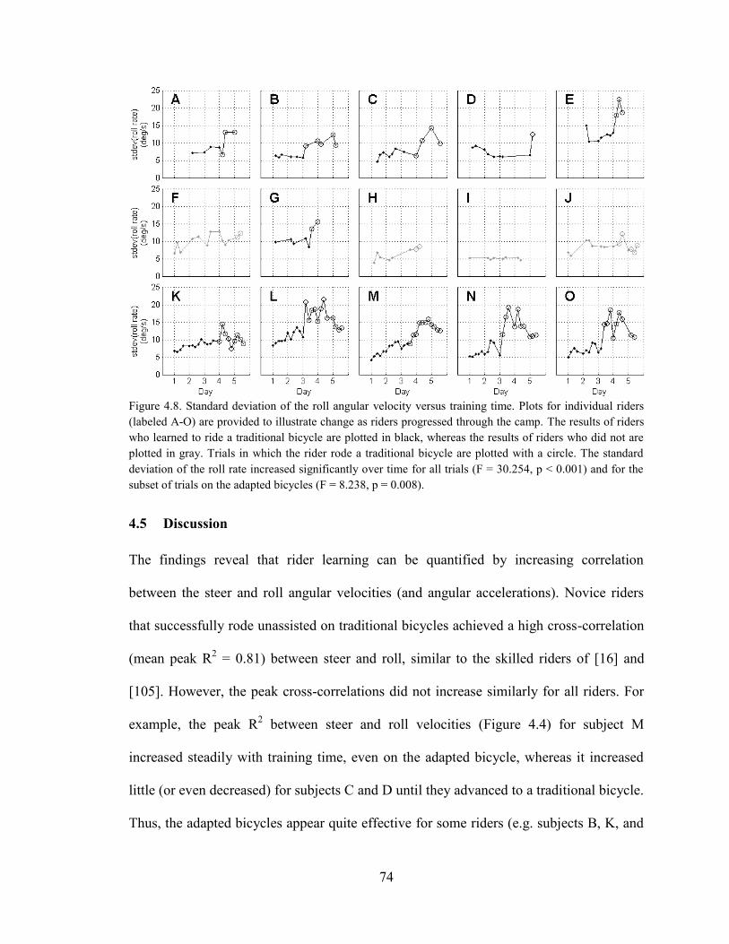
74
Figure 4.8. Standard deviation of the roll angular velocity versus training time. Plots for individual riders
(labeled A-O) are provided to illustrate change as riders progressed through the camp. The results of riders
who learned to ride a traditional bicycle are plotted in black, whereas the results of riders who did not are
plotted in gray. Trials in which the rider rode a traditional bicycle are plotted with a circle. The standard
deviation of the roll rate increased significantly over time for all trials (F = 30.254, p < 0.001) and for the
subset of trials on the adapted bicycles (F = 8.238, p = 0.008).
4.5 Discussion
The findings reveal that rider learning can be quantified by increasing correlation
between the steer and roll angular velocities (and angular accelerations). Novice riders
that successfully rode unassisted on traditional bicycles achieved a high cross-correlation
(mean peak R2 = 0.81) between steer and roll, similar to the skilled riders of [16] and
[105]. However, the peak cross-correlations did not increase similarly for all riders. For
example, the peak R2 between steer and roll velocities (Figure 4.4) for subject M
increased steadily with training time, even on the adapted bicycle, whereas it increased
little (or even decreased) for subjects C and D until they advanced to a traditional bicycle.
Thus, the adapted bicycles appear quite effective for some riders (e.g. subjects B, K, and
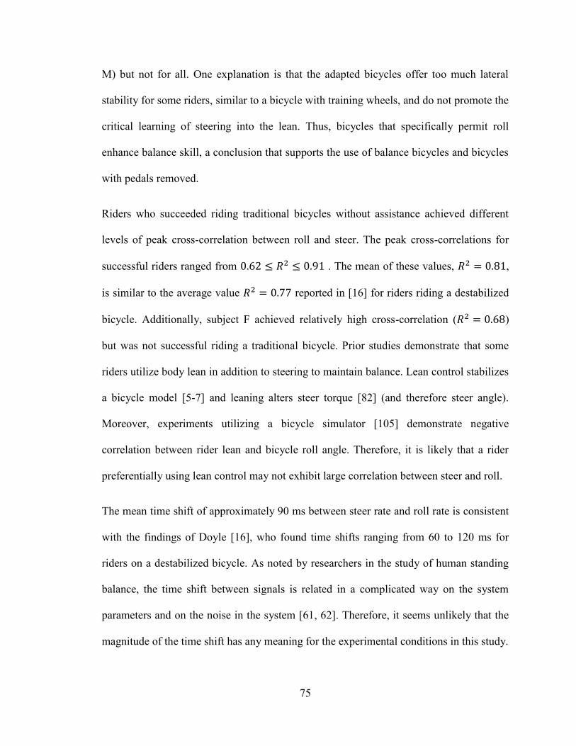
75
M) but not for all. One explanation is that the adapted bicycles offer too much lateral
stability for some riders, similar to a bicycle with training wheels, and do not promote the
critical learning of steering into the lean. Thus, bicycles that specifically permit roll
enhance balance skill, a conclusion that supports the use of balance bicycles and bicycles
with pedals removed.
Riders who succeeded riding traditional bicycles without assistance achieved different
levels of peak cross-correlation between roll and steer. The peak cross-correlations for
successful riders ranged from . The mean of these values, ,
is similar to the average value reported in [16] for riders riding a destabilized
bicycle. Additionally, subject F achieved relatively high cross-correlation ( )
but was not successful riding a traditional bicycle. Prior studies demonstrate that some
riders utilize body lean in addition to steering to maintain balance. Lean control stabilizes
a bicycle model [5-7] and leaning alters steer torque [82] (and therefore steer angle).
Moreover, experiments utilizing a bicycle simulator [105] demonstrate negative
correlation between rider lean and bicycle roll angle. Therefore, it is likely that a rider
preferentially using lean control may not exhibit large correlation between steer and roll.
The mean time shift of approximately 90 ms between steer rate and roll rate is consistent
with the findings of Doyle [16], who found time shifts ranging from 60 to 120 ms for
riders on a destabilized bicycle. As noted by researchers in the study of human standing
balance, the time shift between signals is related in a complicated way on the system
parameters and on the noise in the system [61, 62]. Therefore, it seems unlikely that the
magnitude of the time shift has any meaning for the experimental conditions in this study.

76
The slopes of the linear fit of steer angular velocity to roll angular velocity and the linear
fit of steer angular acceleration to roll angular acceleration increased with training time.
However, it is unclear whether this is due to the riders learning to control the bicycles to
maintain balance, the increased speed that riders exhibit as they progress through the
camp, or due to different dynamic properties of the adapted bicycles. Our results in
Chapter 5 demonstrate that the slope decreases with increasing speed, so it is unlikely
that the observed increase in this study is related to the increased speed that riders exhibit
with training.
As expected, changes in the gearing and the progression from a very stable adapted
bicycle to a traditional bicycle were reflected in changes in the average speed and roll
rate. Higher gearing results in faster average speeds on the adapted bicycles, and the
transition to a traditional bike results in even faster speeds. More crowned rollers
theoretically allow the adapted bicycles to tip more, which can result in increased bicycle
roll rate. Our results demonstrate that the standard deviation of roll rate does increase
with training time, and therefore support the hypothesis transitioning to less stable
bicycles increases the roll rates of the bicycles. However, it may be possible that the
increased roll rate is an effect of the faster average speeds that riders achieve with
increased training. Faster speeds make it possible for a rider to create higher lateral
acceleration for a given steer angle, which would result in higher roll rates. Additionally,
the standard deviation of the steer rate increased with time, suggesting that initially
fearful riders learn to relax their arms and use the handlebars to control and balance the
bicycles. The increased steer rates are also likely a result of the subjects responding to
increased roll rates.

77
There are a few limitations to this study. First, the measurements were taken on a
population with disabilities, which includes subjects with Down syndrome, cerebral
palsy, autism spectrum disorder, and attention deficit hyperactivity disorder. It is not
clear how useful the measurements will be for a non-affected population. However, the
primary finding that steer must be highly correlated to roll is in agreement with past
studies [16, 105, 110] on non-affected populations. Children with disabilities such as
Down syndrome and autism spectrum disorder have motor deficits that may make it
difficult to learn new motor skills [111, 112]. Despite learning deficits, children with
disabilities must still learn the same skill as non-affected children in order to balance a
bicycle. Therefore, we are confident in our conclusion that riding a bicycle requires a
high correlation between steer and roll.
A second limitation is that measurements were taken on modified bicycles (the adapted
bicycles) that are not available to the general public. It is not clear to what degree the
adapted bicycles influence or limit performance measures or how the performance
measures translate to other training techniques. The dynamics and controls approach used
to develop the adapted bicycles has also been applied to develop an ‘unrideable’ bicycle
as well as a bicycle similar to the unrideable bicycle that was made easily rideable by
using a bicycle model to guide slight design modifications [18]. Therefore, all of the
bicycles (adapted and traditional) have very similar dynamic properties. The main effect
of the adapted bicycles seems to be that they reduce the correlation between steer and roll
needed to maintain balance. The rear roller on the adapted bicycle functions similar to
training wheels, providing a corrective force that allows a rider to maintain balance
despite incorrect steering inputs. Unlike training wheels, the adapted bicycles maintain

78
the ability to roll. Our belief is that the adapted bicycles make it possible for riders to
learn incrementally, which is in contrast to the typical fail/succeed nature of learning to
ride a traditional bicycle. The incremental learning that riders demonstrate when using
the adapted bicycles made it possible to capture the learning process.
Learning to balance a bicycle is only one part of learning to ride. Riders must also learn
how to get on a bicycle, how to start pedaling/riding, how to avoid obstacles, and how to
stop safely, among other skills. The primary benefit of adapted bicycles and other
training aids are that they allow riders to become familiar with the controls of a bicycle
and the attention and physical demands that riding a bicycle requires. Adapted bicycles
and balance bikes allow riders to focus on learning the dynamics of a bicycle, whereas
training wheels and tricycles allow riders to learn pedaling, steering, and traffic skills.
Our results suggest several measures that could be used to quantify the learning of novice
riders—especially the peak cross-correlation between steer and roll rates and angular
accelerations. Most importantly, we were able to quantify learning by measuring the
kinematics of bicycles as a riders trained uninterrupted. These measures could be used to
evaluate the effectiveness of existing training techniques and to help develop new
training techniques.
4.6 Conclusions
We measured the essential bicycle kinematics of childern with disabilities during a
specialized bicycle training camp to unravel how they learn to ride bicycles. Of the 15
subjects, 11 successfully rode a traditional bicycle without assistance by the end of the
camp. Three wireless IMUs revealed the bicycle roll rate, steer rate, and speed during the
79
learning process. The peak value of the cross-correlation between steer and roll angular
velocities was significantly greater for the 11 subjects who learned to ride compared to
the 4 who did not. This finding suggests that rider learning is quantified by increased
correlation between bicycle steer rate and roll rate. In essence, learning to steer in the
direction of lean is an essential and quantifiable skill in learning to ride. Average speed
also increased with time, likely due to the increased gearing used as a rider progressed
through the camp. The standard deviation of the steer rate also increased with time,
suggesting that initially fearful riders learn to relax their arms and use the handlebars to
balance the bicycles. Existing and future training techniques can be systematically
evaluated using this novel method.
Acknowledgements
We thank Lose the Training Wheels for providing access to the adapted bicycles and
training program and the National Institute on Disability and Rehabilitation Research for
a grant to Dr. Dale A. Ulrich that made this research possible.

80
CHAPTER 5: MEASUREMENT OF HUMAN/BICYCLE BALANCING DYNAMICS AND
RIDER SKILL
5.1 Chapter summary
Analytical analyses of the stability of bicycle/rider systems have limited use for
understanding the behavior and performance of human bicycle riders and human/bicycle
systems. Experimental measurements of human/bicycle dynamics are needed to advance
our understanding of how humans maintain balance of a bicycle and to identify metrics
useful for quantifying rider skill. In this study, we measure the dynamics of human
bicycle riding as 14 subjects ride an instrumented bicycle on training rollers mounted on
a force platform at speeds ranging from approximately 1.3 to 7.2 m/s. Of the 14 riders,
we classified 7 as cyclists (skilled riders) and 7 as non-cyclists (novice riders). The
instrumented bicycle measures steer angle/rate, steer torque, bicycle speed, and bicycle
roll rate and also enables the calculation of steering power. A motion capture system
enables measurement of the roll angle of the bicycle. A force platform beneath the roller
assembly measures the net force and moment that the bicycle/rider/rollers exert on the
floor, which enables calculation of the lateral positions of the bicycle/rider center of mass
and center of pressure. We find that the cross-correlation of the lateral position of the
center of mass to the lateral position of the center of pressure quantifies balance
performance, the cross-correlation of steer angle/rate to bicycle roll angle/rate quantifies
steer control, and the cross-correlation of rider lean angle to the bicycle roll angle
quantifies rider lean control. All riders achieved similar balance performance at the

81
lowest speed while utilizing similar control strategies. However at higher speeds, skilled
riders (cyclists) achieved greater balance performance by employing more rider lean
control and less steer control compared to novice riders (non-cyclists). In addition, skilled
riders used less steer control effort (measured by average positive steering power and
standard deviations of steer angle and rate) and less rider lean control effort (measured by
the standard deviation of the rider lean angle) regardless of speed. The reduction in
balance effort for skilled riders is not due to any reduced demands for balance. In
summary, skilled riders achieve higher levels of balance performance using less effort
than novice riders.
5.2 Introduction
There is little understanding of the fundamental characteristics of human bicycle riders,
the types of control that humans use to balance bicycles, and the skills that distinguish
riders of different ability levels. Humans have ridden bicycles (two-wheeled, single track
vehicles) since the early 1800’s [1], yet human/bicycle dynamics are far from well
understood. Recent work [2] has established the so-called Whipple bicycle model [3] as
the simplest model of a bicycle that can predict the self-stability of the bicycle alone;
however the behavior of an uncontrolled bicycle provides little insight into the behavior
of a bicycle controlled by a human. Identifying the types of control that humans use and
differences between skilled and novice riders would simultaneously advance two uses.
First, it would provide researchers with metrics to evaluate rider skill and human/bicycle
stability; and second, it could provide bicycle designers with tools to objectively measure
whether a specific bicycle is better or worse for a particular rider.
82
Bicycle riding skill or performance has previously been assessed by instructing subjects
to ride around a prescribed course or to perform a prescribed task. In general, the time to
complete a course/task and the number of errors committed are used to quantify
performance. In the majority of studies that use these techniques, the goal has been to
evaluate the performance or safety of a particular bicycle or bicycle configuration [35-
40]. In a study investigating the maneuverability of children’s bicycles [40], Lewis noted
that there was more variation between subjects than between the use of different bicycles.
The time to complete a course and number of errors were used to investigate the
correlation between physical and perceptual-motor abilities and riding performance [41,
42] and to evaluate the effect of alcohol consumption on the ability to safely ride a
bicycle [43]. While quantifying performance by time to complete a course/task and the
number of errors is useful for the questions posed in these studies, the study results are
task specific and do not translate to new tasks. In addition, the methods of quantifying
performance do not allow continuous monitoring of skill because the methods rely on
completion of specific courses/tasks.
Some research on motorcycles suggests that riders of different skill levels use different
body lean relative to the motorcycle and steering torque. For example, Rice [44] found
that riders of different skill levels phased body lean and steering torque differently when
executing a lane change maneuver. Similarly, Prem [45] found that novice riders in an
evasive maneuver used lean torque and steering torque differently from expert riders.
Prem also used skill tests to differentiate rider ability, similar to the studies of bicycles
mentioned above. However, these studies also provide little insight on how to
continuously monitor skill for bicycle riders.

83
The ability to balance a bicycle is necessary to successfully complete any riding task.
Therefore, it seems logical to investigate possible ways to quantitatively evaluate the skill
of a rider to balance a bicycle. Other fields of research have investigated human
balancing skills and performance and these may also provide insight into how bicycle
balancing skill can be quantified. One such field is human postural control.
The tools used to evaluate human postural control are an essential part of both clinical
evaluation of patients and research into how humans maintain upright posture. Some of
the most basic methods to evaluate human postural control involve monitoring the
location of the center of pressure (COP) and the center of mass (COM) of subjects [47].
During standing, the center of mass and center of pressure are highly correlated, with the
center of pressure being below and tracking the center of mass [113]. By using an ideal
inverted pendulum model of standing balance, Winter [47] explains that the (COP-COM)
signal is directly related to the horizontal acceleration of the COM and can be considered
to be the error signal detected by the balance control system. The assumption is that the
goal of the balance control system is to maintain an upright posture and to control
postural sway. While the assumption that human standing balance can be modeled
effectively as an inverted pendulum, it is important to note that more complex balancing
tasks require a more comprehensive model of the body [48]. Researchers have used COP
measurements to investigate standing balance using a wide range of measures, including:
root mean square (RMS) distance from the mean COP [49, 50], excursions of the COP
[51-53], COP sway amplitude [54], velocity of the COP [55, 56], and the area enclosed
by the COP trajectory [55, 57], among others. These studies represent a small sample of
the extensive literature in the field of human postural control that utilize measures of

84
body sway, usually movement of the COP, to quantify balance performance. As a result,
these types of measures are utilized by clinicians to identify patients with balance
disorders [47, 63, 65].
Similar to research in the field of human postural control, our aim is to identify methods
to evaluate human/bicycle control and balance. Studies of human postural control
highlight the importance of the relationship between the center of mass and center of
pressure. However unlike standing balance, balancing a bicycle is a highly dynamic task
that also requires coordination of the human subject and the bicycle. For standing in static
situations, stability requires that the vertical projection of the center of mass falls within
the base of support; during more dynamic tasks, the projection of the center of mass can
fall outside of the base of support, but must remain within some range of the base of the
support [76]. By logical extension, it will be important to investigate the relationship of
the center of mass to the center of pressure during bicycling.
Previous work highlights possible control methods that can be used by riders [82, 114],
methods to quantify control [16, 105, 107], and differences between skilled and unskilled
riders [115]. Lean control and steer control are effective methods to maintain stability of
a bicycle model [5-7] and are observed experimentally for human riders [24, 114]. Lean
control can also be used to alter steer torque [82], which can in turn alter steer angle.
Both lean control and steer control can be observed by calculating cross-correlations of
lean angle and steer angle/rate with bicycle roll angle/rate [16, 105]. Our pilot experiment
found that skilled cyclists steer less and use less power to steer than non-skilled cyclists
[115], suggesting that the effort used for control as well as variation of control can be
used to distinguish rider skill.

85
Following from the pilot study, the objectives of this study are three-fold: to quantify 1)
the relationship between center of pressure and center of mass movement of the
bicycle/rider system, 2) the types of control used by riders, and 3) the differences
between skilled and novice riders. We hypothesize that the lateral position of the center
of mass will be highly correlated to the lateral position of the center of pressure, steer rate
will be highly correlated to the roll rate of the bicycle, rider lean will be highly correlated
to bicycle roll, and skilled riders will use significantly less steering effort and variation
than novice riders. We open with the Methods section describing the experimental
protocol, the instrumentation used to measure human/bicycle dynamics, and data
analysis. In the Results and Discussion section, we present the results and quantify
differences between skilled and novice riders by highlighting the relationship of the
center of mass to the center of pressure, types of control used, and control effort.
5.3 Methods
We tested a total of 14 subjects (4 females, 10 males; age = 26.4 ± 6.0 years, body mass =
71.1 ± 12.8 kg; mean ± standard deviation). The University of Michigan Health Sciences
and Behavioral Sciences Institutional Review Board approved the study, and all subjects
gave informed consent.
We classified seven subjects as “cyclists” and seven subjects as “non-cyclists.” All
cyclists go on training rides regularly, belong to a cycling club or team, compete several
times per year, and have experience using rollers for training. Skilled riders often use
training rollers, such as those illustrated in Figure 5.1, to practice cycling indoors. All
subjects classified as cyclists identify themselves as skilled cyclists. All non-cyclists
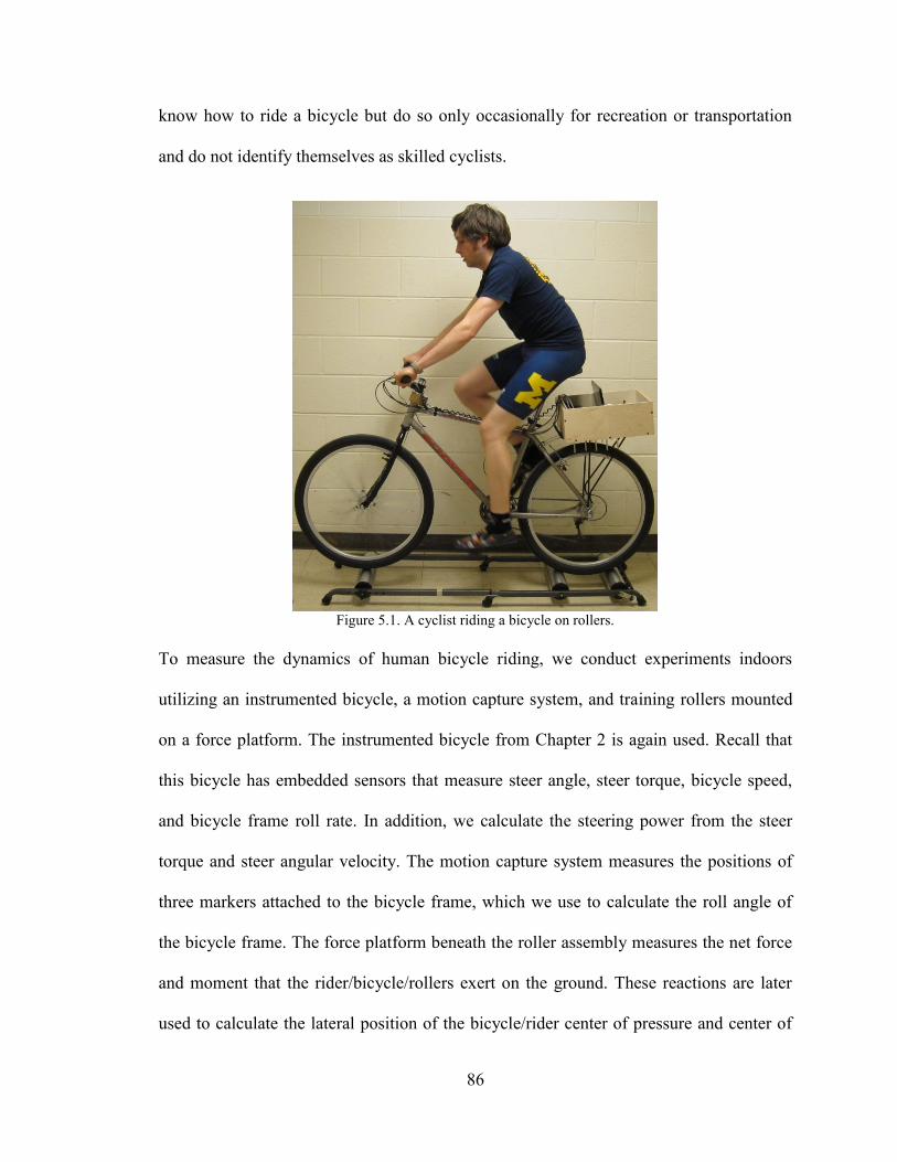
86
know how to ride a bicycle but do so only occasionally for recreation or transportation
and do not identify themselves as skilled cyclists.
Figure 5.1. A cyclist riding a bicycle on rollers.
To measure the dynamics of human bicycle riding, we conduct experiments indoors
utilizing an instrumented bicycle, a motion capture system, and training rollers mounted
on a force platform. The instrumented bicycle from Chapter 2 is again used. Recall that
this bicycle has embedded sensors that measure steer angle, steer torque, bicycle speed,
and bicycle frame roll rate. In addition, we calculate the steering power from the steer
torque and steer angular velocity. The motion capture system measures the positions of
three markers attached to the bicycle frame, which we use to calculate the roll angle of
the bicycle frame. The force platform beneath the roller assembly measures the net force
and moment that the rider/bicycle/rollers exert on the ground. These reactions are later
used to calculate the lateral position of the bicycle/rider center of pressure and center of

87
mass. Utilizing the measured and calculated quantities, we examine standard deviations
of signals and cross-correlations between signals to reveal differences in rider skill.
Protocol 5.3.1
Each subject rode in five experimental conditions distinguished by pedaling cadence (via
a metronome) and bicycle speed (via gearing). The five conditions were executed in the
following order: 1) cadence 80 rpm and speed 5.08 m/s, 2) cadence 80 rpm and speed
7.19 m/s, 3) cadence 80 rpm and speed 6.98 m/s, 4) cadence 80 rpm and speed 2.58 m/s,
and 5) cadence 40 rpm and speed 1.29 m/s. Each subject rode for a minimum of 2
minutes in each condition until s/he could ride for at least 30 seconds without support. A
platform placed over the rollers allows subjects to safely dismount the bicycle and a
railing beside the rollers allows subjects to support themselves during trials (Figure 5.2).
Some subjects were not able to successfully ride on the rollers at the slowest speed
defined in condition 5, and instead rode with a cadence of 50 rpm and a speed of 1.61
m/s. We only instructed riders to ride on the rollers for at least 30 seconds without
support and to match their pedaling rate to the beat of the metronome as closely as
possible. We did not, for example, instruct riders on how to ride the rollers or what type
of control to use.

88
Figure 5.2. A platform placed over the rollers allows subjects to safely dismount the bicycle and a railing
beside the rollers allows subjects to support themselves during trials. The roller drums are mounted to a
frame that is attached to a force platform near the center of the assembly.
Prior to the data collection, we allowed all subjects to practice riding the instrumented
bicycle on the rollers as long as they needed to become comfortable. During this time, we
also ensured that the seat height was set properly for each subject. Cyclists generally
needed only a few minutes to familiarize themselves with the instrumented bicycle. Non-
cyclists, all of whom had no experience riding on rollers, generally needed 10 to 15
minutes to become familiar with the bicycle and to learn how to ride on rollers.
Instrumented bicycle 5.3.2
The instrumented bicycle is described in detail in Chapter 2 and [81, 82]. The
instrumented bicycle is a standard geometry rigid (no suspension) mountain bike
equipped with slick tires. A torque sensor (Transducer Techniques SWS-20) integrated
into the fork steerer tube measures the steer torque applied by the bicycle rider ( ) with a
range of ±7.512 Nm and a resolution of 0.005 Nm. An optical encoder disk (US Digital
HUBDISK-2-1800-1125-I) and encoder module (US Digital EM1-2-1800) capture the

89
steer angle of the bicycle ( ) with a resolution of 0.1 degrees. Numerical differentiation
of the steer angle yields steer angle velocity ( ), which when multiplied by steer torque
yields the instantaneous power used by the rider to steer the bicycle. Integration of
steering power yields the steering work which is further decomposed into positive and
negative work components. We obtain the bicycle speed ( ) by using the measured
circumference of the front wheel and wheel revolutions recorded using a magnetic reed
switch and magnet (Cateye 169-9772 and 169-9691). A three-axis accelerometer (Analog
Devices ADXL335) and three single-axis angular rate gyros (Murata ENC-03M) measure
the acceleration of the bicycle frame with a range and resolution of ±29.43 and
0.067m/s2, respectively, and the angular velocity of the bicycle frame with a range and
resolution of ±300 deg/s and 3.04 deg/s, respectively. From the measured accelerations
and angular velocities, we calculate the bicycle roll rate ( ) as described in Chapter 4.
We sample all signals at 1000 Hz except the steer angle, which is sampled at 200 Hz.
Motion capture system 5.3.3
A motion capture system (Optotrak 3020, Northern Digital Inc.) measures the positions
of three markers rigidly attached to the headtube of the instrumented bicycle (Figure 5.3)
at a sampling rate of 750 Hz. We apply a low-pass filter with a cut-off frequency of 10
Hz to the position data. Using three markers allows us to calculate roll, pitch, and yaw of
the bicycle frame relative to an inertial frame. For this study, only the roll angle is
required. We calculate the roll angle of the bicycle per:
( | |
) (5.1)
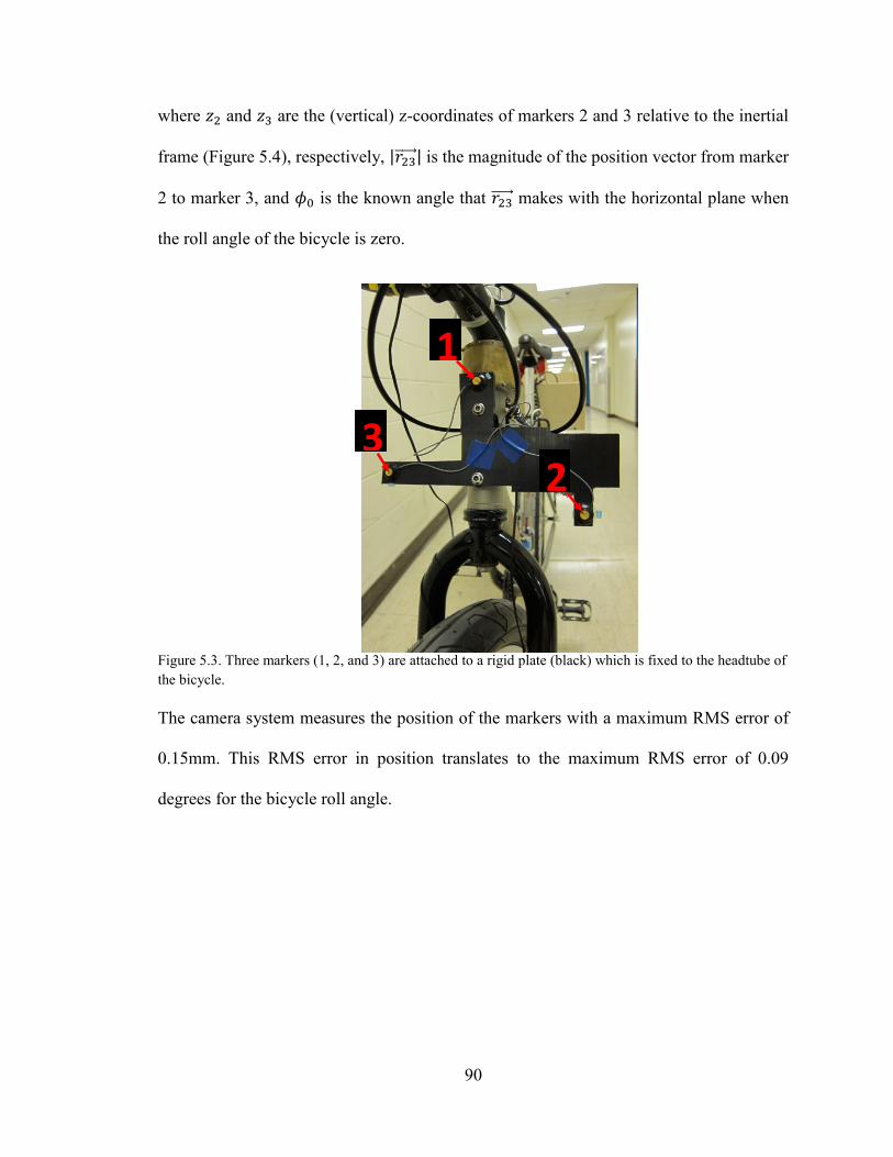
90
where and are the (vertical) z-coordinates of markers 2 and 3 relative to the inertial
frame (Figure 5.4), respectively, | | is the magnitude of the position vector from marker
2 to marker 3, and is the known angle that makes with the horizontal plane when
the roll angle of the bicycle is zero.
Figure 5.3. Three markers (1, 2, and 3) are attached to a rigid plate (black) which is fixed to the headtube of
the bicycle.
The camera system measures the position of the markers with a maximum RMS error of
0.15mm. This RMS error in position translates to the maximum RMS error of 0.09
degrees for the bicycle roll angle.
1
2 3
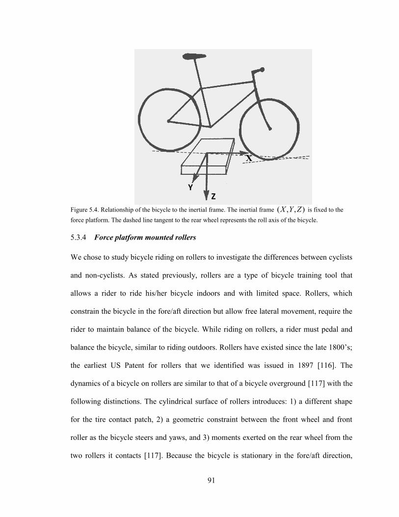
91
Figure 5.4. Relationship of the bicycle to the inertial frame. The inertial frame ),,( ZYX is fixed to the
force platform. The dashed line tangent to the rear wheel represents the roll axis of the bicycle.
Force platform mounted rollers 5.3.4
We chose to study bicycle riding on rollers to investigate the differences between cyclists
and non-cyclists. As stated previously, rollers are a type of bicycle training tool that
allows a rider to ride his/her bicycle indoors and with limited space. Rollers, which
constrain the bicycle in the fore/aft direction but allow free lateral movement, require the
rider to maintain balance of the bicycle. While riding on rollers, a rider must pedal and
balance the bicycle, similar to riding outdoors. Rollers have existed since the late 1800’s;
the earliest US Patent for rollers that we identified was issued in 1897 [116]. The
dynamics of a bicycle on rollers are similar to that of a bicycle overground [117] with the
following distinctions. The cylindrical surface of rollers introduces: 1) a different shape
for the tire contact patch, 2) a geometric constraint between the front wheel and front
roller as the bicycle steers and yaws, and 3) moments exerted on the rear wheel from the
two rollers it contacts [117]. Because the bicycle is stationary in the fore/aft direction,
X
Y Z
92
riders do not experience the same visual cues riding rollers as they do when riding
outdoors.
Rollers offer distinct advantages for investigating human/bicycle dynamics. Most
importantly, rollers allow one to study bicycle riding in a laboratory setting.
Alternatively, one could also employ a treadmill as in [24, 114, 118]. However, rollers
weigh less than a treadmill which is advantageous when also mounting to a force
platform, which often places strict size limits on ground reactions. In addition, riding on
rollers is a safer task than riding on a treadmill. On a treadmill, a rider must carefully
maintain both fore/aft and lateral positions, whereas on rollers a rider only needs to
maintain lateral position. Stopping riding on rollers poses none of the risks of stopping on
a (moving) treadmill. Riding a bicycle on rollers is also more challenging than riding
overground, and therefore may be particularly useful in eliciting differences between
skilled riders (cyclists) and less skilled riders (non-cyclists).
We designed and constructed custom rollers (Figure 5.5 and Figure 5.6) to be mounted on
a force platform (OR6-5-2000, Advanced Mechanical Technology, Inc.). The custom
rollers consist of commercially available drums and belt (Kreitler Challenger 4.5,
Mountain Racing Products) and a frame built from aluminum T-slotted framing (15
Series T-slotted aluminum and joining plates, 80/20 Inc.). The drums selected for the
custom rollers are the largest diameter commercially available. We specifically chose
these rollers because larger drums produce less rolling resistance (making it easier for
subjects to pedal) and are easier to balance a bicycle on than smaller drums [119]. The
construction of the frame allows the rollers to be mounted to a force platform (Figure 5.7)
so that the ground reactions acting on the bicycle/rider/roller system can be measured.

93
Figure 5.5. The custom rollers.
Figure 5.6. The custom rollers.
Figure 5.7. The rollers are designed to be bolted to a force platform. Four brackets on the base of the rollers
are used to secure the rollers to the force platform using four bolts.

94
Figure 5.8. The front roller can be adjusted to ensure that the bicycle is level (adjustment up and down) and
to ensure that the roller contacts the front tire appropriately (adjustment fore and aft).
Figure 5.9. A photograph of the instrumented bicycle on the custom rollers. Note that the bicycle is leaning
against the wall to stay upright.
The design of the custom rollers allows adjustment of both the horizontal and vertical
position of the front roller (Figure 5.8), which allows the bicycle to be level (vertical
adjustment) and to allow the front roller to contact the front wheel directly below the
95
front axle (horizontal adjustment). When a bicycle rolls overground, the ground contacts
the front wheel directly below the front axle of the wheel. Adjusting the front roller
appropriately ensures that controlling the bicycle on rollers is similar to riding
overground.
Calculation of center of pressure and center of mass positions 5.3.5
We utilize the force and moment measurements from the force platform (OR6-5-2000,
Advanced Mechanical Technology, Inc.) to calculate the bicycle/rider/roller center of
pressure (COP) and center of mass (COM) locations in the lateral or y-direction. We
sample all six channels from the force platform at 1000 Hz. After bolting the rollers to
the force platform, we zero all signals. In addition, we also include about 10 seconds of
data at the beginning of each trial so that offsets can be identified and removed during
post-processing. We apply a low-pass filter with a cut-off frequency of 10 Hz to the
measured forces and moments.
The center of pressure is calculated as follows:
( )
(5.2)
( )
(5.3)
where and are the coordinates of the center of pressure, , , and are
forces measured by the force platform, and are moments measured by the force
platform, and is the vertical distance from the origin of the force platform coordinate
system to the plane representing the surface that the bicycle is riding on. The surface is

96
defined by a horizontal plane tangent to the top surface of front roller. Equations (5.2)
and (5.3) assume that the force platform and rollers represent a single rigid body and that
there is no couple applied about the x or y axis; creating a pure couple about the x or y
axis would require attachment of the bicycle to the rollers. We only are interested in the
lateral position of the center of pressure, in the subsequent analysis
To calculate the lateral position of the bicycle/rider center of mass ( ), we implement
a zero-point-to-zero-point integration technique [120, 121] that is a proven for evaluating
postural control [120, 122, 123]. Double integration of the bicycle/rider lateral
acceleration ( ) yields displacement of the bicycle/rider center of mass; however, the
initial constants of integration (initial velocity and initial position) are not known. The
zero-point-to-zero-point integration method is based on the assumption that when the
lateral force is zero ( ), the horizontal position of the gravity line and the center of
pressure coincide ( ). By integrating from one zero point to another zero
point, both the initial velocity and position can be determined. The zero-point-to-zero-
point integration technique is not the only method that can be used to estimate the center
of mass displacement using force platform measurements; other methods utilize dynamic
models of the balancing system and specific filtering techniques [124-127].
Using force platform data to estimate the center of mass position (kinetics-based method)
has several advantages over using a motion capture data (kinematic-based method).
Kinematic-based methods rely on modeling the human body with a number of rigid body
segments. By estimating the mass properties of each segment, usually using
anthropometric data [128], the position of the total-body center of mass can be calculated
if the location and orientation of each segment is known [113, 129]. Kinematic-based
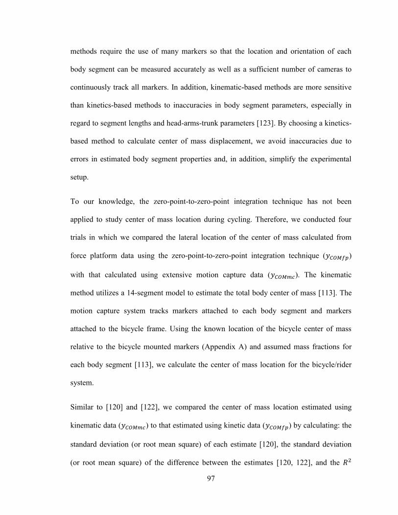
97
methods require the use of many markers so that the location and orientation of each
body segment can be measured accurately as well as a sufficient number of cameras to
continuously track all markers. In addition, kinematic-based methods are more sensitive
than kinetics-based methods to inaccuracies in body segment parameters, especially in
regard to segment lengths and head-arms-trunk parameters [123]. By choosing a kinetics-
based method to calculate center of mass displacement, we avoid inaccuracies due to
errors in estimated body segment properties and, in addition, simplify the experimental
setup.
To our knowledge, the zero-point-to-zero-point integration technique has not been
applied to study center of mass location during cycling. Therefore, we conducted four
trials in which we compared the lateral location of the center of mass calculated from
force platform data using the zero-point-to-zero-point integration technique ( )
with that calculated using extensive motion capture data ( ). The kinematic
method utilizes a 14-segment model to estimate the total body center of mass [113]. The
motion capture system tracks markers attached to each body segment and markers
attached to the bicycle frame. Using the known location of the bicycle center of mass
relative to the bicycle mounted markers (Appendix A) and assumed mass fractions for
each body segment [113], we calculate the center of mass location for the bicycle/rider
system.
Similar to [120] and [122], we compared the center of mass location estimated using
kinematic data ( ) to that estimated using kinetic data ( ) by calculating: the
standard deviation (or root mean square) of each estimate [120], the standard deviation
(or root mean square) of the difference between the estimates [120, 122], and the

98
correlation between the estimates [120]. In addition, we also calculated the slope of the
least squares linear fit of to . In an attempt to quantify the accuracy of the
kinematic method estimate of the center of mass location, we numerically differentiated
the center of mass lateral position twice to obtain the lateral acceleration of the center of
mass ( ) and compared the result to the lateral acceleration calculated from the
force platform data ( , measured lateral force divided by the mass of the
bicycle/rider system). Similar to the center of mass comparisons, we compared the
signals by calculating the correlation and the slope of the least squares linear fit of
to . Table 5.1 summarizes the results of these comparisons.
Table 5.1. Comparison of kinematic-based and kinetics-based estimates of center of mass location and
acceleration.
trial stdev
(yCOMmc)
stdev
(yCOMfp)
stdev
(yCOMmc - yCOMfp)
R2
(yCOMmc, yCOMfp)
slope
(yCOMmc,yCOMfp)
R2
(ÿCOMfp,ÿCOMmc)
slope
(ÿCOMfp,ÿCOMmc)
1 16.8 mm 26.2 mm 13.0 mm 0.825 1.41 0.387 0.36
2 17.0 mm 24.7 mm 10.5 mm 0.881 1.37 0.461 0.45
3 22.3 mm 31.5 mm 11.9 mm 0.921 1.36 0.574 0.66
4 18.1 mm 26.1 mm 10.2 mm 0.917 1.38 0.705 0.60
Similar to the findings of [120], we find that is highly correlated to . In
[120], the authors report cross-correlations ( ) between the kinetics-based method to the
kinematic-based method ranging from 0.79 to 0.96, which translate into correlation
values between 0.62 and 0.92. Therefore, the cross-correlation results indicate that
utilizing the zero-point-to-zero-point integration technique for bicycle riding seems to be
as good if not better than using the technique for postural analysis. As evidenced by the
standard deviations of and and the slope of the linear fit of to
, the kinetics-based approach results in estimates of approximately 40%
greater than the kinematic-based approach, with an RMS difference of about 11mm;
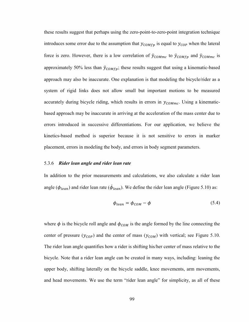
99
these results suggest that perhaps using the zero-point-to-zero-point integration technique
introduces some error due to the assumption that is equal to when the lateral
force is zero. However, there is a low correlation of to and is
approximately 50% less than ; these results suggest that using a kinematic-based
approach may also be inaccurate. One explanation is that modeling the bicycle/rider as a
system of rigid links does not allow small but important motions to be measured
accurately during bicycle riding, which results in errors in . Using a kinematic-
based approach may be inaccurate in arriving at the acceleration of the mass center due to
errors introduced in successive differentiations. For our application, we believe the
kinetics-based method is superior because it is not sensitive to errors in marker
placement, errors in modeling the body, and errors in body segment parameters.
Rider lean angle and rider lean rate 5.3.6
In addition to the prior measurements and calculations, we also calculate a rider lean
angle ( ) and rider lean rate ( ). We define the rider lean angle (Figure 5.10) as:
(5.4)
where is the bicycle roll angle and is the angle formed by the line connecting the
center of pressure ( ) and the center of mass ( ) with vertical; see Figure 5.10.
The rider lean angle quantifies how a rider is shifting his/her center of mass relative to the
bicycle. Note that a rider lean angle can be created in many ways, including: leaning the
upper body, shifting laterally on the bicycle saddle, knee movements, arm movements,
and head movements. We use the term “rider lean angle” for simplicity, as all of these

100
motions can have the effect of moving a rider’s center of mass outside of the plane of the
bicycle frame. The center of mass roll angle, , is computed via
(
) (5.5)
where is the lateral position of the center of pressure, is the lateral position of
the center of mass, and is the location of the bicycle/rider center of mass in the z-
direction when the bicycle and rider are upright, as described and as measured in
Appendix A and [82]. The rider lean rate ( ) is calculated from the rider lean angle
( ) via numerical differentiation.
Figure 5.10. Rider lean as viewed from behind the bicycle/rider. The rider lean angle quantifies how a rider
is shifting his/her center of mass relative to the bicycle. The arrows define the positive sense of all angles.
Rider lean )( lean is defined as the center of mass roll angle )( COM minus the bicycle roll angle )( .
For the example illustrated, the rider lean angle is negative.

101
Selection of data for analysis 5.3.7
As discussed in Section 5.3.1, each subject rode continuously for at least 30 seconds in
each trial. To identify periods of continuous riding, we examined plots of: vertical force
measured by the force platform ( ), steer torque ( ), and bicycle speed ( ). We use
bicycle speed to identify when a subject is pedaling. Inspection of the vertical force
reveals when a subject is supported by the railing or platform (decrease in vertical force).
Examination of the steer torque also identifies periods that a subject uses the railing for
support (oscillations decrease, non-zero offset). After identifying a period of continuous
riding, we use only the last 30 seconds of each period for analysis.
Statistics 5.3.8
In order to quantify rider skill, we looked at the standard deviations of signals, cross-
correlations between signals, and linear relationships between cross-correlated signals.
Normalized cross-correlations [15] are calculated using the xcorr function in the
MATLAB Signal Processing Toolbox. For a given pair of signals, we square the peak
value of the normalized cross-correlation to yield the peak coefficient of determination,
or value, between the two signals. The value provides a measure of the similarity
between the pair of signals. The time shift between two signals required to produce the
peak value provides a measure of the lag or delay before a change in one signal is
correlated to a change in the other signal. Using the time shift for peak correlation
between a pair of signals, we calculate the linear least-squares fit. The slope of the linear
fit can be thought of as a simple gain between signals. We use the following notation for
these quantities:

102
standard deviation of a signal: stdev(signal)
peak value of the normalized cross-correlation of signal 2 to signal 1: (signal 1,
signal 2)
time shift of signal 2 to signal 1: lag(signal 1, signal 2)
slope of linear least-squares fit of signal 2 to signal 1: slope(signal 1, signal 2)
We performed our statistical analyses using an alpha level of 5% ( ). We use
mixed linear models [109] (allowing us to account for repeated measures and unequal
variances) implemented using a statistics software package (IBM SPSS Statistics) to test
for significant effects. We assume an auto regressive covariance model with an order of
one and performed our statistical analyses using an alpha level of 5% ( ). The
models include effects of rider type (cyclist or non-cyclist), speed, and the interaction of
rider type with speed. This approach yields two linear fits (one for each rider type) for
each dependent variable. Including the effect of rider type allows each fit to have a
different y-intercept, and including the rider type/speed interaction allows each fit to have
a different slope. Therefore, significant effects of either rider type or the rider type/speed
interaction indicate significant differences between cyclists and non-cyclists.
5.4 Results and Discussion
We present the experimental results in Figure 5.11 through Figure 5.23; statistical results
are summarized in Table 5.2. We begin by examining the relationship of the center of
mass to the center of pressure and then investigate the types of control used by riders.

103
After presenting these results, we discuss the differences between cyclists and non-
cyclists.
Table 5.2. Summary of statistical tests. Significant effects are denoted with an asterisk (*).
Dependent Variable
Effects
rider type speed rider type*speed
F p F p F p
( ) 13.904 *0.001 114.264 *< 0.001 2.316 0.136
( ) 15.121 *< 0.001 32.223 *< 0.001 0.728 0.397
( ) 24.866 *< 0.001 10.870 *0.002 2.439 0.124
( ) 12.081 *0.001 0.650 0.800 0.813 0.372
( ) 5.304 *0.027 31.998 *< 0.001 7.753 *0.007
( ) 19.643 *< 0.001 4.885 *0.031 0.750 0.390
( ) 3.106 0.086 9.013 *0.004 7.402 *0.009
( ) 3.695 0.059 25.294 *< 0.001 0.037 0.848
( ) 2.483 0.120 29.458 *< 0.001 0.627 0.431
( ) 1.501 0.228 214.928 *< 0.001 10.951 *0.002
( ) 0.036 0.851 30.815 *< 0.001 3.617 0.063
( ) 0.632 0.432 167.203 *< 0.001 1.481 0.230
( ) 0.411 0.526 34.307 *< 0.001 4.650 *0.035
( ) 0.799 0.377 10.357 *0.002 1.624 0.208
( ) 0.673 0.417 142.123 *< 0.001 1.269 0.266
( ) 0.182 0.672 32.948 *< 0.001 17.639 *< 0.001
( ) 0.015 0.902 7.973 *0.006 6.981 *0.010
( ) 0.017 0.896 19.220 *< 0.001 13.865 *< 0.001
( ) 0.863 0.359 1.336 0.252 5.211 *0.026
( ) 2.457 0.125 0.069 0.793 0.969 0.330
( ) 0.852 0.362 43.120 *< 0.001 12.613 *0.001
( ) 0.041 0.841 29.113 *< 0.001 14.843 *< 0.001
( ) 0.000 0.998 11.352 *0.001 11.263 *0.001
average positive steering power 19.213 *< 0.001 10.547 *0.002 1.743 0.194
normalized average positive steering power 25.108 *< 0.001 51.694 *< 0.001 10.612 *0.002
Relationship between the center of mass and center of pressure 5.4.1
For a perfectly balanced bicycle/rider traveling in a straight line, we would expect
to exactly equal . However during actual bicycle riding, similar to human standing,
will not always be exactly equal to . Instead, we expect that the center of mass

104
will track the center of pressure. Figure 5.11 illustrates, using a representative trial, that
the center of mass does indeed track the center of pressure during bicycle riding.
Figure 5.11. Lateral (y) center of pressure location and center of mass location versus time. Data from a
representative trial (non-cyclist, 7.46 m/s) demonstrates the lateral center of mass location closely
tracks the lateral center of pressure location during bicycle riding.
We quantify balance performance by calculating the cross-correlation ( ) and the slope
of the linear least-squares fit of the center of mass location ( ) to the center of
pressure location ( ). For a perfectly balanced bicycle, both and the slope would
be equal to one (1.0). For actual bicycle riding, the values are less than one. Figure 5.12
and Figure 5.13 illustrate these findings.

105
Figure 5.12. Cross-correlation of the lateral position of the center of mass to the center of pressure versus
speed. The cross-correlation decreases significantly with increasing speed (F = 29.113, p < 0.001) and
decreases significantly more with increasing speed for non-cyclists than cyclists (F = 14.843, p < 0.001).
As expected, the lateral positions of the center of mass and center of pressure are highly
correlated during bicycle riding (Figure 5.12). Our data do not indicate a significant
effect of rider type (F = 0.041, p = 0.841; see Table 5.2), but do show significant effects
for both speed (F = 29.113, p < 0.001) and the rider type/speed interaction (F = 14.843, p
< 0.001). All riders demonstrate high correlation at low speeds. As speed increases,
cyclists maintain higher correlation than non-cyclists. Also as expected, the slope of the
linear fit of to is close to one during bicycle riding (Figure 5.13). Similar to
the ( ) results, the slope does not exhibit a significant effect of rider type (F
= 0.000, p = 0.998) but there are significant effects of both speed (F = 11.342, p = 0.001)
and the rider type/speed interaction (F = 11.263, p = 0.001). Again, cyclists and non-
cyclists have slopes close to one at low speeds but the slopes for the non-cyclists
diminish significantly at increased speeds. Our findings suggest that riders with higher

106
skill (cyclists) maintain a higher correlation between lateral center of mass and center of
pressure positions than less-skilled riders (non-cyclists) across all speeds.
Figure 5.13. Slope of the linear fit of the lateral position of the center of mass to the center of pressure
versus speed. The slope decreases significantly with increasing speed (F = 11.352, p = 0.001) and decreases
significantly more for non-cyclists than cyclists (F = 11.263, p = 0.001).
Steering 5.4.2
Bicycle riders utilize two primary control inputs to maintain balance during riding:
steering and leaning. Here we investigate how cyclists and non-cyclists utilize steering.
Subsequently, we turn attention to rider lean; see Section 5.4.3. As expected, we observe
that the steer angle (or steer rate) lags and is correlated to the bicycle roll angle (or roll
rate) during riding (Figure 5.14). Similar to the methods used in Chapter 4, we quantify
steer control by calculating the cross-correlations between steer angles/rates and bicycle
roll angles/rates and the slopes of the linear fits of steer angles/rates to bicycle roll
angles/rates.

107
Figure 5.14. Bicycle roll rate and steer rate versus time. Data from a representative trial (non-cyclist, v
7.96 m/s) demonstrates that the steer rate ( ) lags and is correlated to the bicycle roll rate ( ) during
riding.
All riders demonstrate significant correlation between steer angle and bicycle roll angle
and also steer rate and bicycle roll rate; Figure 5.15 illustrates the results for the cross-
correlation of steer rate to bicycle roll rate. The cross-correlation of steer rate to bicycle
roll rate (Figure 5.15) decreases significantly with increasing speed (F = 34.307, p <
0.001) and decreases significantly more with increasing speed for cyclists than non-
cyclists (F = 4.650, p = 0.035). The cross-correlation of steer angle to bicycle roll angle
results (Table 5.2) are similar to the results for angular rates; the cross-correlation
decreases significantly with increasing speed (F = 214.928, p < 0.001) and decreases
significantly more for cyclists than non-cyclists (F = 10.951, p = 0.002). The peak cross-
correlations between steer and bicycle roll rates for the riders in this study are somewhat
less than those exhibited by riders who just learned to ride a bicycle (Chapter 4). There
are no significant differences between cyclists and non-cyclists in the slope of the linear
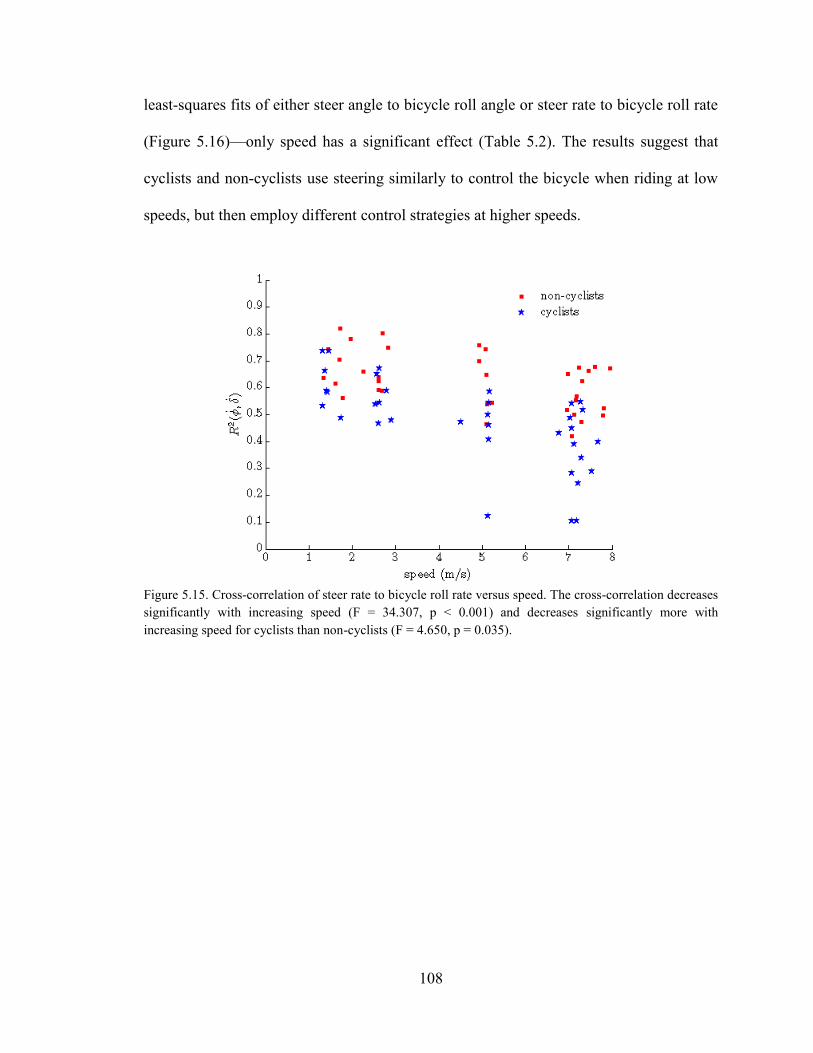
108
least-squares fits of either steer angle to bicycle roll angle or steer rate to bicycle roll rate
(Figure 5.16)—only speed has a significant effect (Table 5.2). The results suggest that
cyclists and non-cyclists use steering similarly to control the bicycle when riding at low
speeds, but then employ different control strategies at higher speeds.
Figure 5.15. Cross-correlation of steer rate to bicycle roll rate versus speed. The cross-correlation decreases
significantly with increasing speed (F = 34.307, p < 0.001) and decreases significantly more with
increasing speed for cyclists than non-cyclists (F = 4.650, p = 0.035).

109
Figure 5.16. Slope of the linear least-squares fit of steer rate to bicycle roll rate versus speed. The slope
decreases significantly with increasing speed (F = 142.123, p < 0.001). There are no significant differences
between cyclists and non-cyclists.
To quantify the steering effort, we calculated the standard deviations of the steer angle
(Figure 5.17) and steer rate (Table 5.2) and average positive steering power (Figure 5.18).
The standard deviations of the steer angle and steer rate and the average positive steering
power decrease significantly with increasing speed for all riders (Table 5.2). These results
are consistent with subject comments that riding at higher speeds seems easier than riding
at lower speeds—lower speeds require more steering effort, as measured by both the
variation of the steer angle and the amount of positive power that a rider must produce for
steering. Our finding that increased speed results in decreased standard deviation of steer
angle is consistent with the results of Moore et al. [114], who found that the variation of
the steer angle decreases with increasing speed for a bicycle ridden on a treadmill.
Cyclists exhibit less variation of steer angle (F = 13.904, p = 0.001), less variation of
steer rate (F = 15.121, p < 0.001), and less positive steering power (F = 19.213, p <

110
0.001) than non-cyclists. The higher skill level of the cyclists enables less steering effort
to maintain balance of the bicycle during riding.
Figure 5.17. Standard deviation of steer angle versus speed. The standard deviation of steer angle decreases
significantly with increasing speed (F = 114.264, p < 0.001). Cyclists exhibit significantly less steer angle
variation than non-cyclists (F = 13.904, p < 0.001).
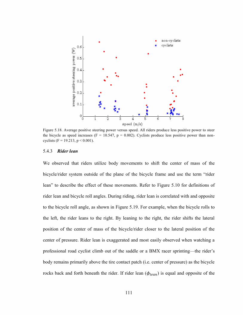
111
Figure 5.18. Average positive steering power versus speed. All riders produce less positive power to steer
the bicycle as speed increases (F = 10.547, p = 0.002). Cyclists produce less positive power than non-
cyclists (F = 19.213, p < 0.001).
Rider lean 5.4.3
We observed that riders utilize body movements to shift the center of mass of the
bicycle/rider system outside of the plane of the bicycle frame and use the term “rider
lean” to describe the effect of these movements. Refer to Figure 5.10 for definitions of
rider lean and bicycle roll angles. During riding, rider lean is correlated with and opposite
to the bicycle roll angle, as shown in Figure 5.19. For example, when the bicycle rolls to
the left, the rider leans to the right. By leaning to the right, the rider shifts the lateral
position of the center of mass of the bicycle/rider closer to the lateral position of the
center of pressure. Rider lean is exaggerated and most easily observed when watching a
professional road cyclist climb out of the saddle or a BMX racer sprinting—the rider’s
body remains primarily above the tire contact patch (i.e. center of pressure) as the bicycle
rocks back and forth beneath the rider. If rider lean ( ) is equal and opposite of the
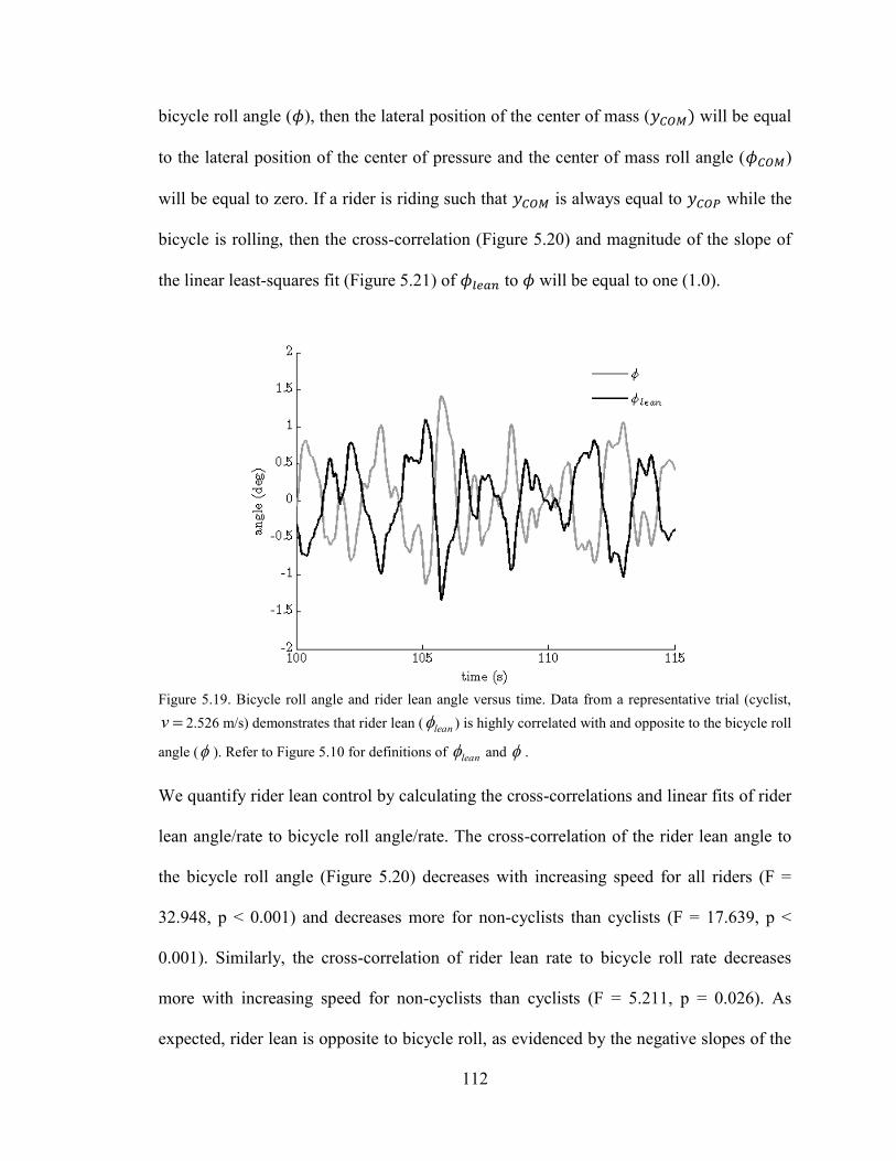
112
bicycle roll angle ( ), then the lateral position of the center of mass ( ) will be equal
to the lateral position of the center of pressure and the center of mass roll angle ( )
will be equal to zero. If a rider is riding such that is always equal to while the
bicycle is rolling, then the cross-correlation (Figure 5.20) and magnitude of the slope of
the linear least-squares fit (Figure 5.21) of to will be equal to one (1.0).
Figure 5.19. Bicycle roll angle and rider lean angle versus time. Data from a representative trial (cyclist,
v 2.526 m/s) demonstrates that rider lean ( lean ) is highly correlated with and opposite to the bicycle roll
angle ( ). Refer to Figure 5.10 for definitions of lean and .
We quantify rider lean control by calculating the cross-correlations and linear fits of rider
lean angle/rate to bicycle roll angle/rate. The cross-correlation of the rider lean angle to
the bicycle roll angle (Figure 5.20) decreases with increasing speed for all riders (F =
32.948, p < 0.001) and decreases more for non-cyclists than cyclists (F = 17.639, p <
0.001). Similarly, the cross-correlation of rider lean rate to bicycle roll rate decreases
more with increasing speed for non-cyclists than cyclists (F = 5.211, p = 0.026). As
expected, rider lean is opposite to bicycle roll, as evidenced by the negative slopes of the

113
linear fits of rider lean angle to bicycle roll angle (Figure 5.21). Both the slopes of the fits
of rider lean to bicycle roll and rider lean rate to bicycle roll rate decrease in magnitude
with increasing speed and decrease in magnitude more for non-cyclists than cyclists
(Table 5.2). Like the findings for steer control, these results suggest that cyclists and non-
cyclists use similar rider lean strategies at low speeds, but use different strategies at
higher speeds.
Figure 5.20. Cross-correlation of rider lean angle to bicycle roll angle versus speed. The cross-correlation
decreases significantly with increasing speed (F = 32.948, p < 0.001) and decreases significantly more with
increasing speed for non-cyclists than cyclists (F = 17.639, p < 0.001).
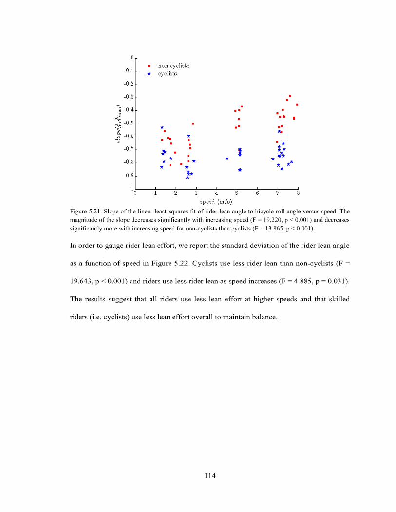
114
Figure 5.21. Slope of the linear least-squares fit of rider lean angle to bicycle roll angle versus speed. The
magnitude of the slope decreases significantly with increasing speed (F = 19.220, p < 0.001) and decreases
significantly more with increasing speed for non-cyclists than cyclists (F = 13.865, p < 0.001).
In order to gauge rider lean effort, we report the standard deviation of the rider lean angle
as a function of speed in Figure 5.22. Cyclists use less rider lean than non-cyclists (F =
19.643, p < 0.001) and riders use less rider lean as speed increases (F = 4.885, p = 0.031).
The results suggest that all riders use less lean effort at higher speeds and that skilled
riders (i.e. cyclists) use less lean effort overall to maintain balance.
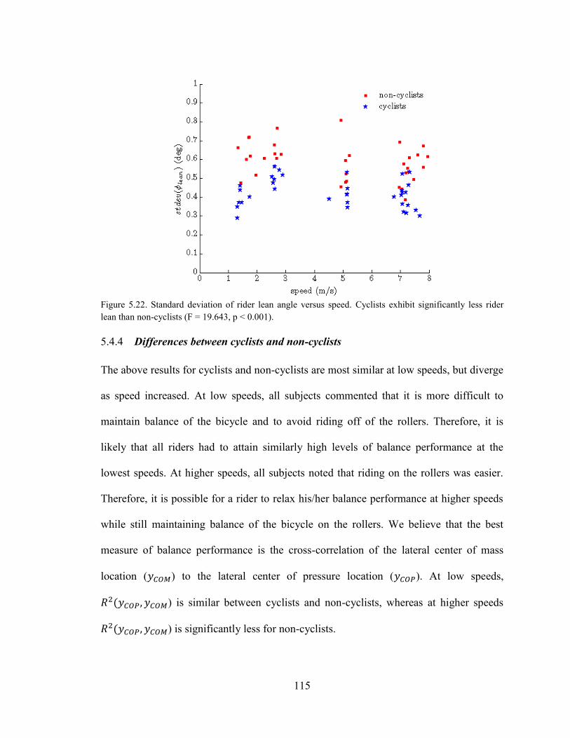
115
Figure 5.22. Standard deviation of rider lean angle versus speed. Cyclists exhibit significantly less rider
lean than non-cyclists (F = 19.643, p < 0.001).
Differences between cyclists and non-cyclists 5.4.4
The above results for cyclists and non-cyclists are most similar at low speeds, but diverge
as speed increased. At low speeds, all subjects commented that it is more difficult to
maintain balance of the bicycle and to avoid riding off of the rollers. Therefore, it is
likely that all riders had to attain similarly high levels of balance performance at the
lowest speeds. At higher speeds, all subjects noted that riding on the rollers was easier.
Therefore, it is possible for a rider to relax his/her balance performance at higher speeds
while still maintaining balance of the bicycle on the rollers. We believe that the best
measure of balance performance is the cross-correlation of the lateral center of mass
location ( ) to the lateral center of pressure location ( ). At low speeds,
( ) is similar between cyclists and non-cyclists, whereas at higher speeds
( ) is significantly less for non-cyclists.

116
To achieve high balance performance, cyclists use a different control strategy than non-
cyclists. We quantified two types of control strategies, steering and rider lean, by
investigating the correlation of steer angle/rate and rider lean angle/rate to bicycle roll
angle/rate. Compared to non-cyclists, cyclists utilize greater rider lean than steering to
maintain balance, especially at higher speeds. Greater rider lean control decreases the
need for additional steer control required to maintain balance. This conclusion is
supported by the above observation that cyclists achieve higher balance performance than
non-cyclists despite exhibiting lower cross-correlation between steer and bicycle roll
rates. In Chapter 4, we hypothesized that some children were able to ride a bicycle with a
lower cross-correlation between steer and bicycle roll rates than other children because
they were utilizing rider lean to control balance in addition to steering; the results of this
study support that hypothesis.
To assess the relative importance of steer versus lean control on balance performance, we
used a mixed linear model to address whether any measures of control (i.e. cross-
correlations) predict the cross-correlation of to , the adopted measure of
balance performance. Again we used an alpha level of 5% and an auto regressive
covariance model with order of one. The dependent variable was ( ) and the
effects were ( ), ( ), ( ), and ( ). Of the tested effects,
only ( ), the cross-correlation of rider lean to the bicycle roll angle, was a
significant predictor of balance performance (F = 84.768, p < 0.001). Therefore, we
conclude that rider lean is the dominant control strategy for balance performance for
riding on rollers. The above results demonstrate that cyclists exploit rider lean control
significantly more than non-cyclists to achieve higher balance performance.
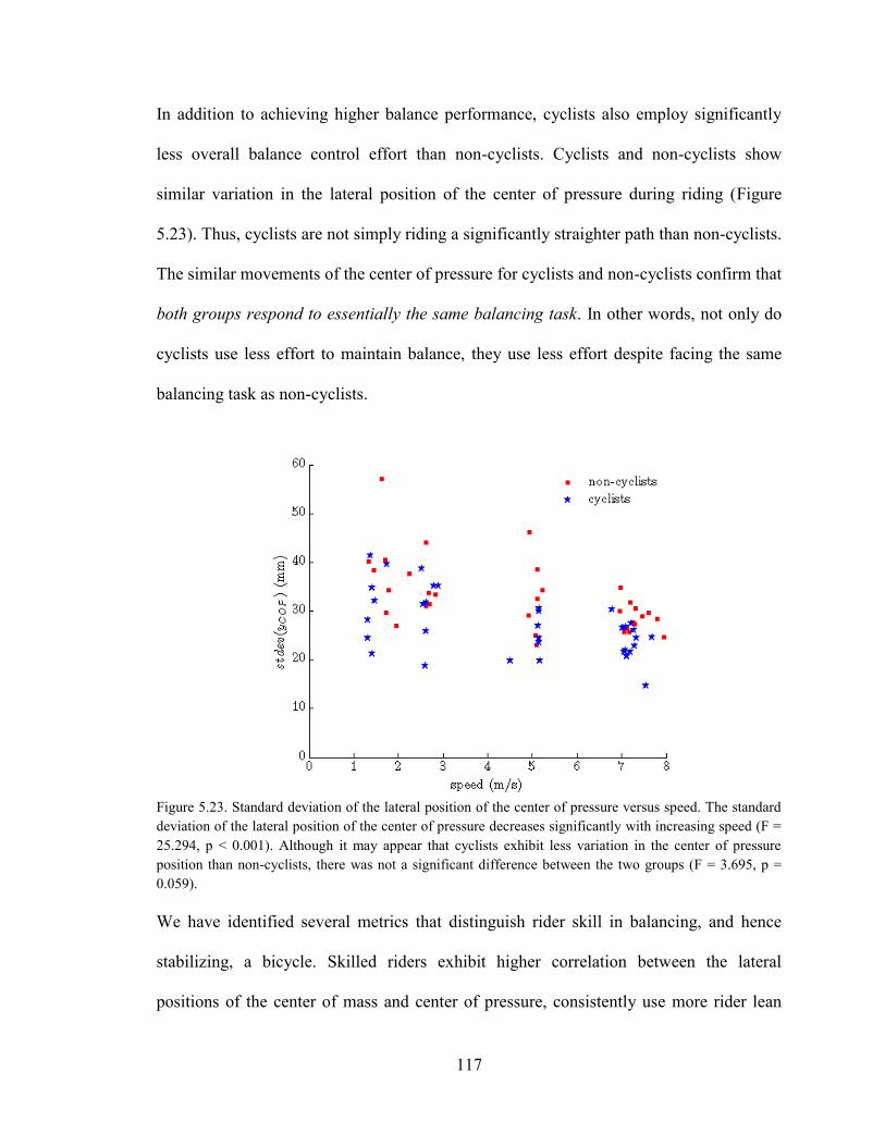
117
In addition to achieving higher balance performance, cyclists also employ significantly
less overall balance control effort than non-cyclists. Cyclists and non-cyclists show
similar variation in the lateral position of the center of pressure during riding (Figure
5.23). Thus, cyclists are not simply riding a significantly straighter path than non-cyclists.
The similar movements of the center of pressure for cyclists and non-cyclists confirm that
both groups respond to essentially the same balancing task. In other words, not only do
cyclists use less effort to maintain balance, they use less effort despite facing the same
balancing task as non-cyclists.
Figure 5.23. Standard deviation of the lateral position of the center of pressure versus speed. The standard
deviation of the lateral position of the center of pressure decreases significantly with increasing speed (F =
25.294, p < 0.001). Although it may appear that cyclists exhibit less variation in the center of pressure
position than non-cyclists, there was not a significant difference between the two groups (F = 3.695, p =
0.059).
We have identified several metrics that distinguish rider skill in balancing, and hence
stabilizing, a bicycle. Skilled riders exhibit higher correlation between the lateral
positions of the center of mass and center of pressure, consistently use more rider lean

118
than less skilled riders, and use significantly less effort than less skilled riders. While
dynamic models of bicycles, such as the Whipple model [3], successfully predict the
stability of an uncontrolled bicycle [12], they ignore the above stabilizing actions of the
human rider. Metrics that define rider skill (such as those above) could become useful for
understanding how bicycle design can influence rider balance performance. For example,
any bicycle designed to help riders maintain balance at low speeds should increase the
cross-correlation between the lateral positions of the center of pressure and center of
mass. Metrics of balance performance could also serve to evaluate the effectiveness of
bicycle training programs. For example, riders with initially poor balancing skills could
undergo a training program (perhaps riding a bicycle on training rollers, as shown in
Figure 5.1) to help improve their skills. By quantifying differences between skilled and
novice riders, we have provided researchers and practitioners with tools to objectively
measure the effects of different bicycle designs on real-life bicycle riding.
5.5 Conclusion
We measured the dynamics of human bicycle riding as 14 subjects rode an instrumented
bicycle on training rollers mounted on a force platform and at speeds ranging from
approximately 1.3 to 7.2 m/s. Of the 14 riders, we classified 7 as cyclists (skilled riders)
and 7 and non-cyclists (novice riders). The instrumented bicycle measured steer
angle/rate, steer torque, bicycle speed, and bicycle roll rate and also enabled the
calculation of steering power. A motion capture system enabled the measurement of the
roll angle of the bicycle. A force plate beneath the roller assembly measured the net force
and moment that the bicycle/rider/rollers exerted on the floor, which also enabled
calculation of the lateral position of the bicycle/rider center of mass and center of

119
pressure. We found that the cross-correlation of the lateral position of the center of mass
to the lateral position of the center of pressure quantifies balance performance, the cross-
correlation of steer angle/rate to bicycle roll angle/rate quantifies steer control, and the
cross-correlation of rider lean angle to the bicycle roll angle quantifies rider lean control.
All riders achieved similar balance performance at the lowest speed while utilizing
similar control strategies. However at higher speeds, skilled riders (cyclists) achieved
greater balance performance by employing more rider lean control and less steer control
compared to novice riders (non-cyclists). In addition, skilled riders used less steer control
effort (measured by average positive steering power and standard deviations of steer
angle and rate) and less rider lean control effort (measured by the standard deviation of
the rider lean angle) regardless of speed. The reduction in balance effort for skilled riders
is not due to any reduced demands for balance. The metrics introduced herein could also
quantify balance performance of the bicycle/rider system in broad contexts including 1)
the analysis of bicycle designs, 2) the performance of assistive technologies, and 3) the
assessment of training programs.

120
CHAPTER 6: SUMMARY AND CONTRIBUTIONS
The overall goal of this dissertation was to advance our understanding of how human
riders control bicycles, the types of control that humans utilize to balance and steer
bicycles, and the skills that distinguish human riders of different ability levels. In order to
achieve this goal, we pursued the following four specific aims:
1. Design and build an instrumented bicycle that is capable of measuring the
primary human control inputs (steer torque and rider lean) and fundamental
bicycle kinematics.
2. Investigate human/bicycle dynamics and control during steady-state turning
using experimental and analytical approaches.
3. Quantify the changes that occur as learners transition from non-riders to
riders.
4. Quantify the differences between skilled and novice riders when balancing a
bicycle.
Below, we discuss each specific aim by providing a brief summary, listing the main
contributions and conclusions, and then discussing some limitations. Major overarching
conclusions drawn from all four studies follow this discussion.
6.1 Summary, contributions, and conclusions of each study
Specific Aim 1: Design and build an instrumented bicycle that is capable of
measuring the primary human control inputs and fundamental bicycle kinematics

121
(Chapter 2). Developing and building an instrumented bicycle was critical to the
completion of this dissertation. In particular, it was important to have a bicycle and
measurement techniques that could be used outside the confines a laboratory. Our
instrumented bicycle measures steer angle, steer torque, angular velocity of the bicycle
frame, acceleration of the bicycle frame, and bicycle speed. Through numerical
differentiation, we obtain steering angular velocity or rate. Multiplication of measured
steering torque by steering rate yields steering power, which quantifies rider steering
effort. During steady-state turning, measurements of the acceleration of the bicycle frame
and the bicycle speed provide an estimate of the bicycle roll angle, which further enables
computation of rider lean angle. The battery-powered sensors and on-board data
acquisition computer are self-contained, which allows the instrumented bicycle to be used
in non-laboratory environments. Additionally, the design does not require any
attachments or special interfaces with the rider. The rider is unconstrained and therefore
free to employ the very same natural movements and control for riding any bicycle.
Specific Aim 1: Major contributions
Designed and constructed a novel instrumented bicycle, which places no
constraints on rider movement and can be used outside of laboratory
environments
Specific Aim 1: Major conclusions
The instrumented bicycle directly measures a primary human control input (steer
torque) and fundamental bicycle kinematics (steer angle, roll rate, and bicycle
speed)
122
Additional measures of human/bicycle dynamics are calculated from the
measured data including the second primary human control input (rider lean) in
addition to other kinematic measures (steering angular rate, steering power,
bicycle roll angle)
The instrumented bicycle is limited in that it measures rider lean and bicycle roll angles
during steady-state turning, not during arbitrary or straight line riding. Conducting riding
tests in a laboratory equipped with a motion capture system allowed us to overcome these
limitations quite easily (Chapter 5); however, there are some elegant solutions that would
allow us to measure the rider lean and bicycle roll angles outside of a laboratory
environment. A simple trailer can be used to measure the roll angle of the bicycle [130];
and both [31] and [45] present simple and inexpensive methods to estimate rider lean
angle using potentiometers. While the trailer would be straight forward to implement, the
proposed methods to measure rider lean angle introduce limitations. Both methods
require a rod to be secured to the rider and only consider rider lean developed from lateral
flexion of the trunk. As demonstrated in [114] and [24], riders use many motions besides
lateral flexion of the trunk to generate what we define as rider lean (lateral shifting of
rider mass center). Therefore, measurements of only lateral flexion of the trunk would
fail to capture many of the motions that we believe are important for maintaining balance
of a bicycle. An extreme approach is to eliminate all rider motion expect for steering
[118, 130].This approach includes using a body orthosis to prevent trunk movement,
eliminating the task of pedaling by using an electric motor to power the bicycle, and
securing the rider’s feet and knees to the bicycle frame to eliminate all leg movement.
Depending on the research question, eliminating all rider motions except steering may be

123
justified. However, our research goal was to understand the natural control humans
employ while riding a bicycle and therefore it was imperative to maintain all control
degrees of freedom.
Specific Aim 2: Investigate human/bicycle dynamics and control during steady-state
turning using experimental and analytical approaches (Chapter 3). The steady-state
turning of a bicycle arises when the bicycle/rider system negotiates a constant radius turn
with constant speed and roll angle. We explored steady-state turning by employing the
instrumented bicycle to measure steering torque, steering angle, and bicycle speed,
acceleration, and angular velocity. We used a model for steady-state turning, based on the
Whipple bicycle model [2, 3], to interpret our results.
Our experimental and analytical investigation of steady-state turning served several
purposes. Consideration of the bicycle/rider system during steady-state turning was our
starting point for understanding basic bicycle/rider dynamics and control. Steady-state
turn testing allowed us to tightly control bicycle speed, turn radius, and rider lean to
assess the effects of these variables on bicycle kinematics (roll and steer angles) and what
has been considered the primary human input to the bicycle (steering torque).
Additionally, because we used a steady-state formulation of the Whipple bicycle model
to interpret our results, we were able to extend the utility of this commonly used model
for predicting the dynamics of human bicycle riding.
In Chapter 3, we reported data obtained from 134 trials using two subjects executing
steady turns defined by nine different radii, three speeds, and three rider lean conditions.
A model for steady-state turning is used to interpret the experimental results. Overall, the
124
model explains 95.6% of the variability in the estimated bicycle roll angle, 99.4% of the
variability in the measured steering angle, and 6.5% of the variability in the measured
steering torque. However, the model explains 56.6% of the variability in steering torque
for the subset of trials without exaggerated rider lean relative to the bicycle frame. Thus,
the model, which assumes a rigid and non-leaning rider, reasonably predicts bicycle/rider
roll and steering angles for all rider lean conditions and steering torque without
exaggerated rider lean. The findings demonstrate that lateral shifting of the bicycle/rider
center of mass strongly influences the steering torque, suggesting that rider lean plays an
important role in bicycle control during steady-state turning. By contrast, the required
steering angle is largely insensitive to rider lean, suggesting that the steering angle serves
as a superior cue for bicycle control relative to steering torque.
Specific Aim 2: Major contributions
Provided novel experimental data for steady-state turning that includes steer
torque, steer angle, and roll angle over a wide range of turn radii, bicycle speeds,
and rider lean conditions
Adapted the Whipple bicycle model for steady-state turning.
Specific Aim 2: Major conclusions
The model, which assumes a rigid and non-leaning rider, successfully predicts
bicycle kinematics (roll and steer angles) for all rider lean conditions
The model only reasonably predicts steering torque for normal riding (no
exaggerated rider lean)

125
Lateral shifting of the bicycle/rider center of mass (i.e. rider lean) strongly
influences steering torque, suggesting that rider lean plays an important role in
bicycle control during steady-state turning
The required steering angle for a given turn radius is largely insensitive to rider
lean, suggesting that steering angle is a better cue for bicycle control than steering
torque
The steady-state turning study has the following limitations. First, we chose to compare
the experimental data to a steady-state turning model based on the Whipple bicycle
model. The primary shortcoming of this model is that it ignores rider lean. Nevertheless,
we chose the Whipple model due to its wide use in bicycle research. As a result, our
results also provide other researchers with data to evaluate the limitations of the Whipple
model for understanding human bicycle riding. In an earlier study [81], we introduced an
alternative, simplified steady-state turning model that explicitly incorporates rider lean.
This model yields more accurate predictions of steering torque than the steady-state
turning version of the Whipple model. The study is also limited because it only considers
two riders and one bicycle design. A more complete study would assess several bicycle
designs and riders. Different bicycle designs could arise from simply turning the fork
backwards, installing different front wheels, and adding weight to different places on the
bicycle to affect the mass distribution and inertia.
Specific Aim 3: Quantify the changes that occur as learners transition from non-
riders to riders (Chapter 4). Riding a bicycle is a skill that many people learn quite
easily as reflected in the common assertion, “it’s as easy as riding a bike.” However,
there is little scientific understanding about how we learn to ride and balance a bicycle.

126
The objective of the study detailed in Chapter 4 was to quantify how human subjects
learn to ride a bicycle by tracking key kinematic changes in bicycle roll and steer
dynamics during the learning process. The subjects for this study were children who
participated in a specialized bicycle training camp called Lose the Training Wheels; refer
to www.losethetrainingwheels.org. Children enter this camp having no ability to ride a
bicycle and either acquire that ability or make significant progress towards that goal by
the end of the week-long camp [46, 106]. Therefore, this camp provides an ideal setting
for tracking the changes that arise as a child transitions from a non-rider to a rider. A
previous analysis of pilot data [107] helped develop our hypotheses and methods. We
hypothesized that the measured bicycle steer and roll angular velocities would become
significantly correlated as a successful subject progressed through training. In addition,
we hypothesized that the average bicycle speed, the standard deviation of the roll angular
velocity, and the standard deviation of the steer angular velocity would all increase with
training.
We measured the fundamental bicycle kinematics of novice riders with disabilities during
the specialized bicycle training camp to unravel how they learn to ride traditional
bicycles. Of the 15 subjects, 11 successfully rode a traditional bicycle without assistance
by the end of the camp. Three wireless IMUs revealed the bicycle roll rate, steer rate, and
speed during the learning process. The peak value of the cross-correlation between steer
and roll angular velocities was significantly greater for the 11 subjects who learned to
ride compared to the 4 who did not. This finding suggests that rider learning is quantified
by increased correlation between bicycle steer rate and roll rate. In essence, learning to
steer in the direction of bicycle lean is an essential and quantifiable skill in learning to
127
ride. Average speed also increased with time, likely due to the increased gearing used as
a rider progressed through the camp. The standard deviation of the steer rate also
increased with time, suggesting that initially fearful riders learn to relax their arms and
use the handlebars to balance the bicycles. As expected, the standard deviation of the
bicycle roll rate also increased with time, likely due to the more crowned rollers that
learners use as they progress towards riding a traditional bicycle. Existing and future
training techniques can be systematically evaluated using this new skill assessment
method.
Specific Aim 3: Major contributions
We developed a novel experimental method utilizing three synchronized inertial
measurement units (IMUs) to measure the bicycle kinematics critical for
understanding rider learning
o The IMUs are easily and quickly mounted to any bicycle
o The IMUs can be reliably used in both indoor and outdoor environments
Specific Aim 3: Major conclusions
Rider learning can be quantified by increasing correlation between the steer and
roll angular velocities (and angular accelerations)
Average speed of the riders increased with training time, likely due to increases in
gearing as riders progress through the camp
Standard deviation of the steer rate increased with time, suggesting that initially
fearful riders learn to relax their arms and use the handlebars to balance the
bicycles

128
Standard deviation of the bicycle roll rate increased with time, likely due to the
more crowned rollers that learners use as they progress towards riding a
traditional bicycle
Learning to steer in the direction of lean is an essential skill in learning to ride a
bicycle
We duly note the following limitations to this study. First, the measurements were taken
on a population with disabilities, which includes subjects with Down syndrome, cerebral
palsy, autism spectrum disorder, and attention deficit hyperactivity disorder. It is not
clear how all of the findings may translate to a non-affected population. However, the
primary finding that steer must be highly correlated to roll is in agreement with past
studies [16, 105, 110] on non-affected populations. Children with disabilities such as
Down syndrome and autism spectrum disorder have motor deficits that may make it
difficult to learn new motor skills [111, 112]. Despite learning deficits, children with
disabilities must still learn the same skill as non-affected children in order to balance a
bicycle. In addition, our results from Chapter 5 demonstrate that non-affected subjects
(cyclists and non-cyclists) also exhibit a high correlation of steer rate to bicycle roll rate.
Therefore, we remain confident in the conclusion that riding a bicycle requires a high
correlation between steer and roll.
A second limitation is that measurements were taken on modified bicycles (the adapted
bicycles) that are not available to the general public. It is not clear to what degree the
adapted bicycles influence or limit performance measures or how the performance
measures translate to other training techniques. The approach used to develop the adapted
bicycles has also been applied to develop an ‘unrideable’ bicycle as well as a bicycle
129
similar to the unrideable bicycle that was made rideable by using a bicycle model to
guide slight design modifications [18]. Therefore, we believe that all of the bicycles (both
adapted and traditional) exhibit very similar dynamic properties. The main effect of the
adapted bicycles is that they reduce the correlation between steer and roll needed to
maintain balance. The rear roller on an adapted bicycle functions similar to training
wheels, providing a corrective force that allows a rider to maintain balance despite
incorrect steering inputs. Unlike training wheels, the adapted bicycles maintain the ability
to roll, albeit with limits on roll. We hypothesize that the adapted bicycles make it
possible for riders to learn incrementally, which is in contrast to the typical fail/succeed
nature of learning to ride a traditional bicycle. The incremental learning that riders
demonstrate when using the adapted bicycles made it possible to capture and study the
learning process.
Specific Aim 4: Quantify the differences between skilled and novice riders when
balancing a bicycle (Chapter 5). There is little understanding of the fundamental
characteristics of human bicycle riders, the types of control that humans use to balance
bicycles, and the skills that distinguish riders of different ability levels. Identifying the
types of control that humans use and differences between skilled and novice riders would
simultaneously advance two uses. First, it would provide researchers with metrics to
evaluate rider skill and human/bicycle stability. Second, it could provide bicycle
designers with tools to objectively measure whether a specific bicycle design enhances or
diminishes the balance skill of a particular rider. The objectives of the study detailed in
Chapter 5 were three-fold: to quantify 1) the relationship between center of pressure and
center of mass movement of the bicycle/rider system, 2) the types of control used by
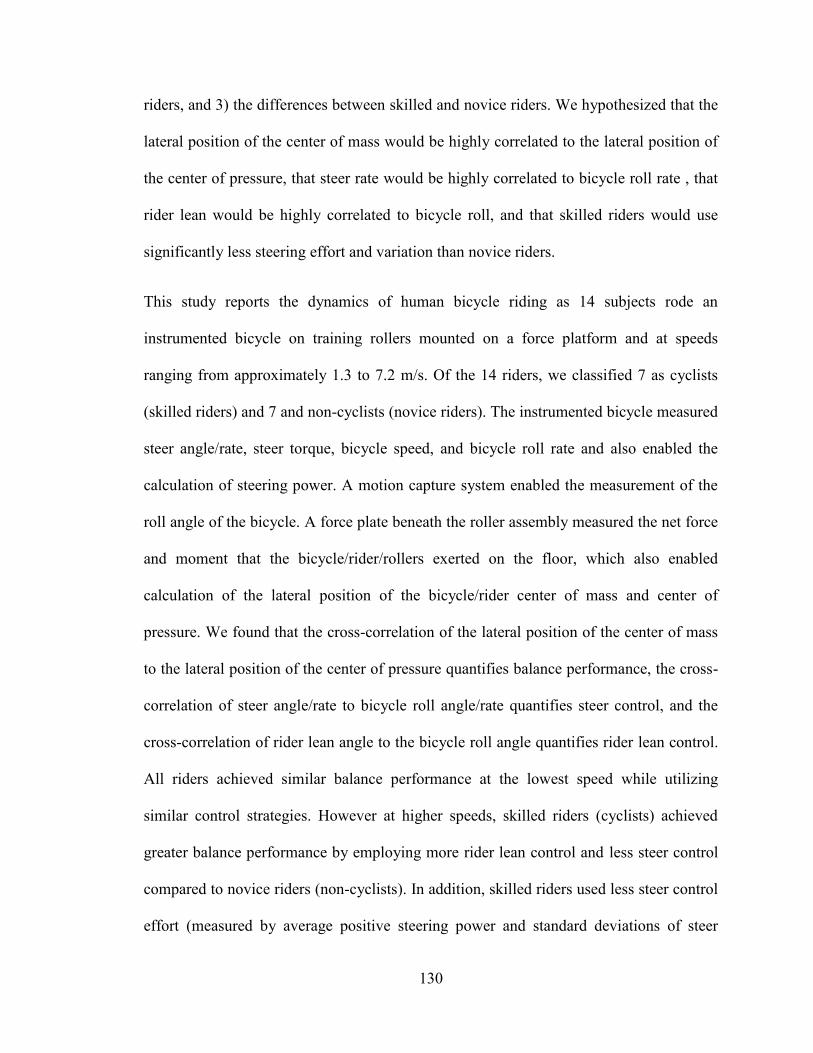
130
riders, and 3) the differences between skilled and novice riders. We hypothesized that the
lateral position of the center of mass would be highly correlated to the lateral position of
the center of pressure, that steer rate would be highly correlated to bicycle roll rate , that
rider lean would be highly correlated to bicycle roll, and that skilled riders would use
significantly less steering effort and variation than novice riders.
This study reports the dynamics of human bicycle riding as 14 subjects rode an
instrumented bicycle on training rollers mounted on a force platform and at speeds
ranging from approximately 1.3 to 7.2 m/s. Of the 14 riders, we classified 7 as cyclists
(skilled riders) and 7 and non-cyclists (novice riders). The instrumented bicycle measured
steer angle/rate, steer torque, bicycle speed, and bicycle roll rate and also enabled the
calculation of steering power. A motion capture system enabled the measurement of the
roll angle of the bicycle. A force plate beneath the roller assembly measured the net force
and moment that the bicycle/rider/rollers exerted on the floor, which also enabled
calculation of the lateral position of the bicycle/rider center of mass and center of
pressure. We found that the cross-correlation of the lateral position of the center of mass
to the lateral position of the center of pressure quantifies balance performance, the cross-
correlation of steer angle/rate to bicycle roll angle/rate quantifies steer control, and the
cross-correlation of rider lean angle to the bicycle roll angle quantifies rider lean control.
All riders achieved similar balance performance at the lowest speed while utilizing
similar control strategies. However at higher speeds, skilled riders (cyclists) achieved
greater balance performance by employing more rider lean control and less steer control
compared to novice riders (non-cyclists). In addition, skilled riders used less steer control
effort (measured by average positive steering power and standard deviations of steer
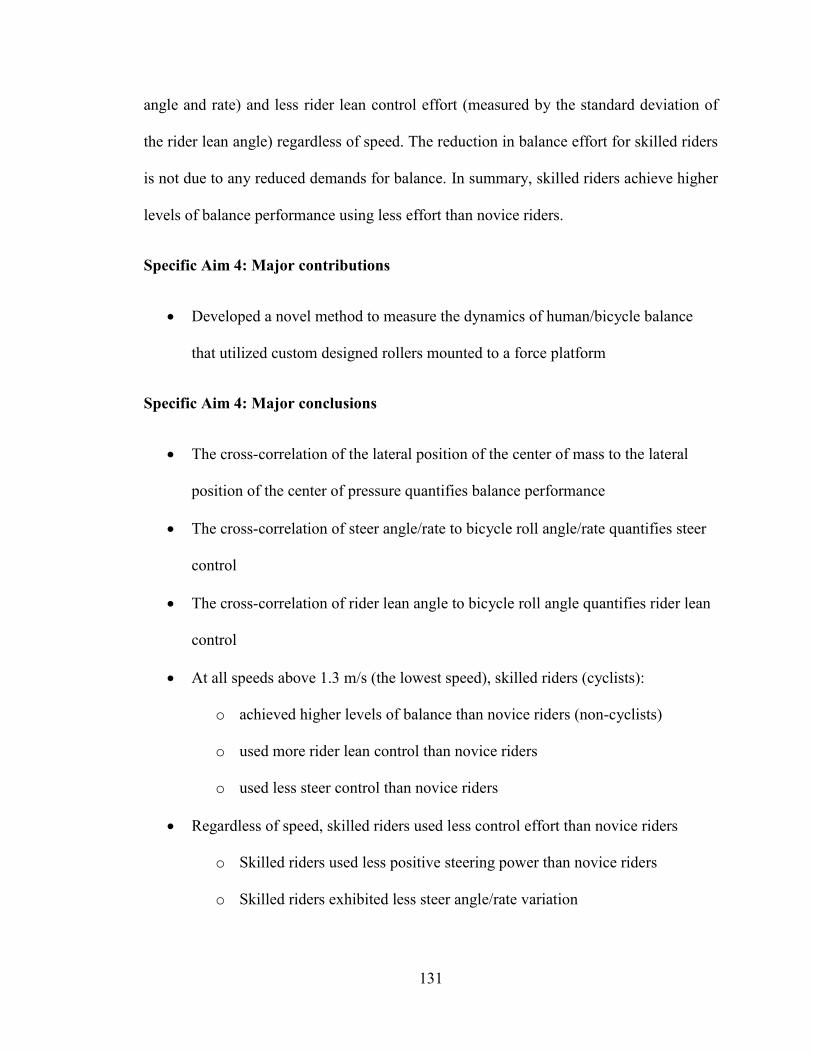
131
angle and rate) and less rider lean control effort (measured by the standard deviation of
the rider lean angle) regardless of speed. The reduction in balance effort for skilled riders
is not due to any reduced demands for balance. In summary, skilled riders achieve higher
levels of balance performance using less effort than novice riders.
Specific Aim 4: Major contributions
Developed a novel method to measure the dynamics of human/bicycle balance
that utilized custom designed rollers mounted to a force platform
Specific Aim 4: Major conclusions
The cross-correlation of the lateral position of the center of mass to the lateral
position of the center of pressure quantifies balance performance
The cross-correlation of steer angle/rate to bicycle roll angle/rate quantifies steer
control
The cross-correlation of rider lean angle to bicycle roll angle quantifies rider lean
control
At all speeds above 1.3 m/s (the lowest speed), skilled riders (cyclists):
o achieved higher levels of balance than novice riders (non-cyclists)
o used more rider lean control than novice riders
o used less steer control than novice riders
Regardless of speed, skilled riders used less control effort than novice riders
o Skilled riders used less positive steering power than novice riders
o Skilled riders exhibited less steer angle/rate variation

132
Our investigation of human/bicycle balancing dynamics is limited by several factors.
First, we chose to conduct our experiments on a custom set of bicycle training rollers.
The relationship of bicycle riding on rollers to riding overground has not been quantified,
and there is some disagreement about the differences and similarities between the two
tasks [117, 131, 132]. Therefore, it is not yet clear if all the metrics that distinguish rider
skill on rollers would also distinguish rider skill overground. We recognized this
limitation before the onset of the study and decided to conduct the experiments on rollers
because of several advantages they present: 1) riding on rollers is more challenging than
riding overground, and therefore this task may be particularly useful in eliciting
differences between skilled riders and less skilled riders, 2) rollers can be easily and
securely mounted to a force platform, and 3) riding on rollers is safer than riding on a
treadmill, which is the primary alternative for studying human/bicycle dynamics in a
laboratory setting. We carefully designed the custom rollers to ensure that the balancing
dynamics would be as similar as possible to riding overground. The adjustable front drum
ensures that the bicycle is level and that the trail of the bicycle is the same on the rollers
as overground. Our choice of the largest diameter drums minimizes differences between
the front tire ground contact when riding on rollers versus when riding overground.
Another final limitation is that subjects were not able to ride their own bicycles—they
were required to ride the instrumented bicycle. While we did adjust the seat height for
each subject and allowed each subject ample time to adjust to the instrumented bicycle,
the fit was not ideal for every subject. The role of bicycle fit on bicycle control has not
been quantified, but it is possible that a non-ideal fit may result in diminished
performance. Despite this limitation, we still were able to detect significant differences

133
between skilled and novice riders and believe that these differences would persist if all
subjects rode their own bicycles.
6.2 Overarching conclusions
While the above studies target different aims, their results highlight two overarching
conclusions.
Overarching conclusion 1: Rider lean (i.e., lateral movement of the rider relative to
the bicycle frame) plays a dominant role in steering and balancing a bicycle.
Theoretical studies demonstrate that rider lean can maintain bicycle stability, even in the
absence of steer control [5-7]. All three studies herein provide experimental evidence that
rider lean is important for balancing and steering a bicycle. In the study on steady-state
turning (Chapter 3), we conclude that lateral shifting of the bicycle/rider center of mass
(i.e. rider lean) strongly influences steering torque. Because steer torque directly
influences steer angle, it follows that a rider can easily influence the steer angle through
leaning. In the study of rider learning (Chapter 4), results demonstrate that not all riders
that learned to ride achieved similarly high levels of cross-correlation between steer and
bicycle roll rates. In particular, some riders achieved very high cross-correlations (R2
=
0.9) whereas others only achieved modest cross-correlations (R2
= 0.7) only slightly
larger than some riders that were not successful riding a bicycle. We hypothesized that a
rider using lean control could reduce the otherwise required correlation between steer and
roll. Our results from the study of rider balance skill (Chapter 5) confirm that a rider can
indeed reduce the required correlation between steer and roll by exploiting rider lean
control. In fact, we found that cross-correlation between rider lean angle and bicycle roll
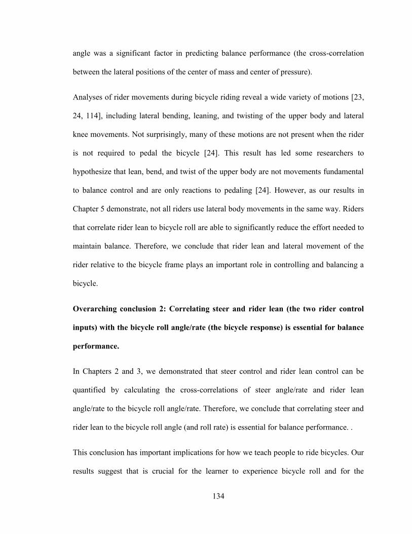
134
angle was a significant factor in predicting balance performance (the cross-correlation
between the lateral positions of the center of mass and center of pressure).
Analyses of rider movements during bicycle riding reveal a wide variety of motions [23,
24, 114], including lateral bending, leaning, and twisting of the upper body and lateral
knee movements. Not surprisingly, many of these motions are not present when the rider
is not required to pedal the bicycle [24]. This result has led some researchers to
hypothesize that lean, bend, and twist of the upper body are not movements fundamental
to balance control and are only reactions to pedaling [24]. However, as our results in
Chapter 5 demonstrate, not all riders use lateral body movements in the same way. Riders
that correlate rider lean to bicycle roll are able to significantly reduce the effort needed to
maintain balance. Therefore, we conclude that rider lean and lateral movement of the
rider relative to the bicycle frame plays an important role in controlling and balancing a
bicycle.
Overarching conclusion 2: Correlating steer and rider lean (the two rider control
inputs) with the bicycle roll angle/rate (the bicycle response) is essential for balance
performance.
In Chapters 2 and 3, we demonstrated that steer control and rider lean control can be
quantified by calculating the cross-correlations of steer angle/rate and rider lean
angle/rate to the bicycle roll angle/rate. Therefore, we conclude that correlating steer and
rider lean to the bicycle roll angle (and roll rate) is essential for balance performance. .
This conclusion has important implications for how we teach people to ride bicycles. Our
results suggest that is crucial for the learner to experience bicycle roll and for the

135
learner’s control actions to affect the roll of a training bicycle in a way similar to a
traditional bicycle. For example, training wheels by design prevent bicycle roll, render it
impossible for the learner to experience bicycle roll, and therefore impossible for the
bicycle to respond similarly to one without training wheels. Without experiencing bicycle
roll and how steering and rider lean affect bicycle roll, the rider has no opportunity to
learn appropriate control actions. Unlike bicycles with training wheels, the adapted
bicycles detailed in Chapter 4 allowed the riders to experience bicycle roll dynamics and
to gradually learn distinctions between correct and incorrect control actions.
Unfortunately for children that use training wheels, learning correct and incorrect control
actions usually occurs only after removal of the training wheels. At that point, the penalty
for a wrong control action is typically a crash. Training wheels are excellent for helping
children learn pedaling and navigation skills, but they are not ideal for teaching balance
skills. Fortunately, society is gradually recognizing the limitations of training wheels, as
evidenced by the recent popularity of balance bikes. Balance bikes or run bikes have no
pedals, drivetrain, or training wheels, and require the rider to kick his/her feet to propel
the bike forward. Because balance bicycles allow bicycle roll, it is possible for the rider
to learn how to correlate steer and rider lean to bicycle roll, which inevitably leads to
successful riding.

136
APPENDIX A: MEASUREMENT OF BICYCLE PARAMETERS
The procedures used to determine the parameters of the instrumented bicycle for the
steady-state turning model (Section 3.3.3) are presented below. These procedures are
guided by previous studies [9, 133-135]. The measured parameters are reported in Table
A.2.
A.1 Wheel base ( w )
With the bicycle secured in an upright position (roll angle = 0 degrees) and with the front
wheel aligned with the plane defined by the bicycle frame (steer angle = 0 degrees), we
measured: the distance from the rear wheel axis to the front wheel axis on both the left
and right sides of the bicycle (with a tape measure, resolution = 0.001 m), the width of
the front axle, and the width of the rear axle (with calipers, resolution = 0.03 mm). We
used the four measurements to define a trapezoid; solving for the height of the trapezoid
yields the length of the wheel base of the bicycle, .
A.2 Wheel radius ( Fr , Rr )
Similar to [9, 133-135], we estimated the radii of the front ( ) and rear ( ) wheels by
measuring the linear distance traveled on the ground through 14 rotations of each wheel.
During each trial, a subject sat on the bicycle (tire pressure = 2.76 bar) with the seat
height adjusted properly as he/she was pushed from behind while making his/her best
effort to follow a straight course. We measured the distance covered in each trial using a
30 m long tape measure (resolution = 1.6 mm). We collected three trials for each wheel

137
for each subject. The measured distances were divided by to obtain the effective
rolling radius for each trial; trials were averaged to obtain values for each wheel for each
subject. The effective rolling radii were not significantly different between subjects.
A.3 Steer axis tilt ( )
We measured the steer axis tilt by securing the bicycle with each subject seated on the
bicycle in an upright position (roll angle = steer angle = 0 degrees) and measuring the
angle of the head tube of the bicycle using a digital inclinometer (resolution = 0.01
degrees). To account for the floor potentially being out of level, we measured the steer
axis tilt with the bicycle in two configurations—the first as described above and the
second simply with the bicycle facing the opposite direction. We took the average of the
two measurements as the steer axis tilt of the loaded bicycle. The steer axis tilt was not
significantly different between subjects.
A.4 Fork rake/offset ( of )
We measured the fork rake (also known as fork offset) as described in [133] and found
the measured fork rake to agree with the rake value provided by the manufacturer to the
nearest millimeter.
A.5 Trail ( c )
Instead of measuring the trail ( ) of the bicycle directly, we calculated the trail using the
following equation [133]:
(A.1)
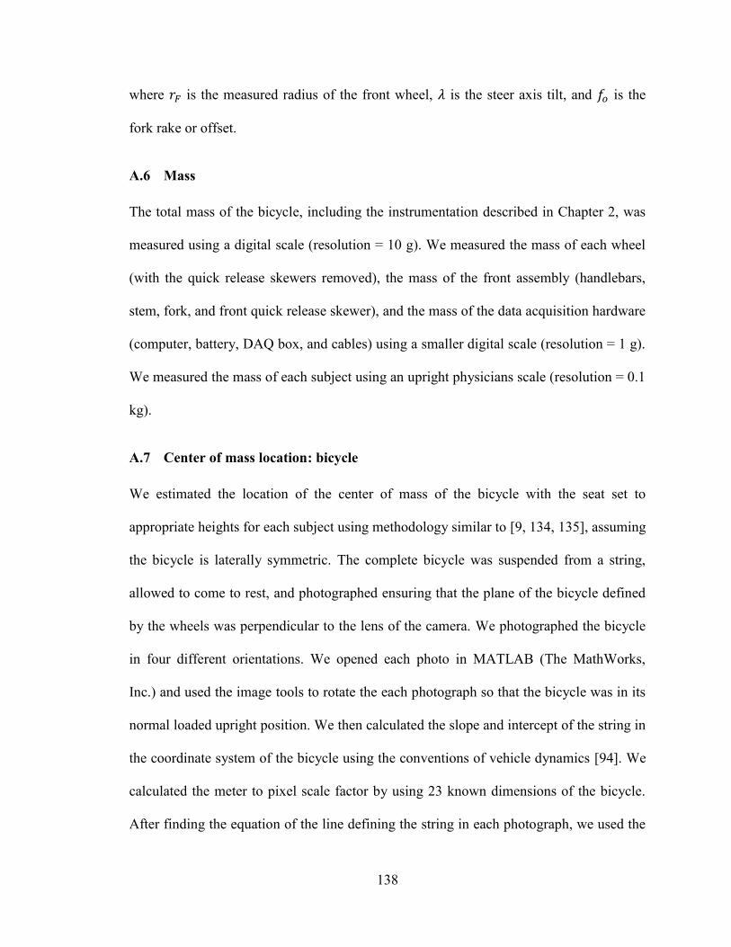
138
where is the measured radius of the front wheel, is the steer axis tilt, and is the
fork rake or offset.
A.6 Mass
The total mass of the bicycle, including the instrumentation described in Chapter 2, was
measured using a digital scale (resolution = 10 g). We measured the mass of each wheel
(with the quick release skewers removed), the mass of the front assembly (handlebars,
stem, fork, and front quick release skewer), and the mass of the data acquisition hardware
(computer, battery, DAQ box, and cables) using a smaller digital scale (resolution = 1 g).
We measured the mass of each subject using an upright physicians scale (resolution = 0.1
kg).
A.7 Center of mass location: bicycle
We estimated the location of the center of mass of the bicycle with the seat set to
appropriate heights for each subject using methodology similar to [9, 134, 135], assuming
the bicycle is laterally symmetric. The complete bicycle was suspended from a string,
allowed to come to rest, and photographed ensuring that the plane of the bicycle defined
by the wheels was perpendicular to the lens of the camera. We photographed the bicycle
in four different orientations. We opened each photo in MATLAB (The MathWorks,
Inc.) and used the image tools to rotate the each photograph so that the bicycle was in its
normal loaded upright position. We then calculated the slope and intercept of the string in
the coordinate system of the bicycle using the conventions of vehicle dynamics [94]. We
calculated the meter to pixel scale factor by using 23 known dimensions of the bicycle.
After finding the equation of the line defining the string in each photograph, we used the
139
least squares method to solve for the intersection of the four lines [133]. The intersection
is the estimated center of mass location for the bicycle. The process was repeated with the
seat height adjusted to the appropriate height for each subject.
A.8 Center of mass location: handlebars, stem, and fork ( Hx , Hz ).
We estimated the center of mass location for the handlebar, stem, and fork assembly
using the methodology described for the bicycle (Section A.7). We suspended the
assembly in four orientations and used nine known dimensions to calculate the meter to
pixel scale factor. The center of mass location was found relative to the front fork dropout
and later converted to coordinates in the bicycle coordinate system.
A.9 Center of mass location: wheels.
The centers of mass of the wheels were assumed to be at their geometrical centers.
A.10 Center of mass location: bicycle and rider ( Tx , Tz )
Similar to the center of mass for the bicycle, we estimated the center of mass location for
the bicycle/rider system for each subject by using photographs. We used the data of both
Clauser et al. [136] and Dempster [128] to estimate the mass properties of the following
13 body segments: head and trunk, two arms, two forearms, two hands, two thighs, two
legs, and two feet. For all segments except the hands, we used the data of [136] to
calculate the mass of each segment (as a percentage of a subject’s total weight) and the
location of the center of mass (as a percentage of the limb length from one end of the
segment). We chose to use the data of [136] because segment lengths are defined relative
to anatomical landmarks that are easily identified by palpation. We calculated the mass of
the hands using data from [136] but used data from [128] to calculate the location of the

140
center of mass; we made this choice because [128] found the center of mass location of
hands with a similar configuration to that of a hand gripping a handlebar whereas [136]
located the center of mass of hands with extended fingers. The values used to estimate
segment properties as well as the landmarks used to identify each segment can be found
in Table A.1.
Table A.1. Body segment properties (from Clauser et al. [136] and Dempster [128]). The mass of each
segment is calculated as a fraction of the body mass and the location of the center of mass of each segment
is calculated as a fraction of the segment length.
Segment (segment mass)
/ (body mass)
(Location of center of
mass from proximal
or superior end of
segment) / (segment
length)
Proximal (superior)
end point
Distal (inferior)
end point
head and
torso 0.580 0.592 vertex of head trochanterion
upper arm 0.026 0.513 acromiale radiale
forearm 0.016 0.390 radiale styloid process of
ulna
hand 0.007 0.506 styloid process of ulna
proximal
interphalangeal
knuckle of finger II
thigh 0.103 0.372 trochanterion tibiale mediale or
tibiale laterale
leg 0.043 0.371 tibiale mediale or
tibiale laterale
sphyrion fibulare or
sphyrion laterale
foot 0.015 0.449 dorsal surface of heel tip of longest toe
Prior to photographing each subject on the bicycle, we used palpation to identify: the
acromiale, radiale, styloid process of the ulna, trochanterion, tibiale mediale, tibiale
laterale, sphyrion fibulare, and sphyrion laterale [137]. After identification, we marked
the location of each landmark with small dots of tape. Each subject then sat on the
instrumented bicycle with the seat height adjusted appropriately. We secured the
bicycle/rider in an upright position (lean angle = steer angle = 0) and photographed the
bicycle/rider from the side, ensuring that the plane of the bicycle defined by the wheels
was perpendicular to the lens of the camera. We opened each photo (one for each subject)

141
in MATLAB and used the image tools to rotate each photograph so that the bicycle was
in its normal loaded upright position. We calculated the meter to pixel scale factor by
using 23 known dimensions of the bicycle. Using the dots of tape as a guide, the locations
of the end points of each segment were digitized. We estimated the location of the
segment centers of mass by using the ratios in Table A.1, assuming that the center of
mass for a segment falls on a line connecting the two endpoints. We calculated the center
of mass locations for the thigh, leg, and foot segments independently for each leg, but
assumed that the left upper arm, forearm, and hand segments were symmetric to the
segments on the right side of the body. Given the center of mass of the segments and the
bicycle (Section A.7), we calculated the rider/bicycle center of mass:
∑
(A.2)
∑
(A.3)
where ( ) is the location of the bicycle/rider system center of mass, is a subscript
denoting a segment or the bicycle, is the total mass of the bicycle/rider system, is
the mass of a segment or the bicycle, and ( ) is the center of mass location of a
segment or the bicycle.
A.11 Inertia of wheels about axles ( FyyI , RyyI )
To measure the mass moment of inertia of a wheel about its axle, we hung the wheel as a
compound pendulum by hanging the wheel from a thin horizontal rod parallel to the
wheel axle [9, 133-135]. We secured a wireless angular rate gyro (InvenSense ITG-3200)

142
to the hub of the wheel with one axis oriented parallel to the axle of the wheel, and
perturbed the wheel to oscillate about the axis of the rod. Using the measured angular rate
about the axis parallel to the wheel axle, we measured the time required for the wheel to
complete 35 oscillations; dividing the time by 35 yields the period ( ) of oscillation. We
measured the period of oscillation for each wheel in six different orientations, and used
the average period for each wheel to calculate the inertia of each wheel about its axle
[134]:
( )
( ) ( ) (A.4)
where is a subscript denoting the front ( ) or rear ( ) wheel, is the time of one
oscillation, is the mass of the wheel, is the mass of the angular rate gyro used
for measurement (25 g), is gravity (9.81 m/sec2), and is the distance from the thin rod
to the center of mass of the wheel (pendulum arm length). We assumed that the distance
was equal to the inner radius of the rim, which we measured using a three-dimensional
digitizing system (MicroScribe G2X, resolution = 0.23mm).
A.12 Calculation of stiffness matrices ( 0K , 2K )
The terms of the two stiffness matrices that appear in our steady-state turning equations
must be calculated from the measured parameters. We calculate the stiffness matrices as
described in [2], and reproduce the equations here for completeness.
First, the mass properties of the front assembly (front wheel, handlebars, and fork) must
be calculated:

143
(A.5)
(A.6)
(A.7)
Next, we calculate the perpendicular distance between the center of mass of the front
assembly and the steering axis:
( ) (A.8)
The ratio of the mechanical trail to the wheel base is given by:
(A.9)
The gyrostatic coefficients are given by:
(A.10)
(A.11)
(A.12)
A frequently appearing static moment term is defined as:
(A.13)
Finally, we can calculate the gravity-dependent stiffness terms:
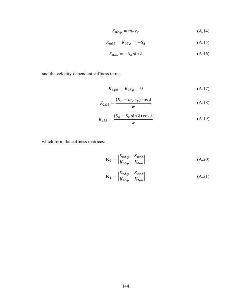
144
(A.14)
(A.15)
(A.16)
and the velocity-dependent stiffness terms:
(A.17)
( )
(A.18)
( )
(A.19)
which form the stiffness matrices:
[
] (A.20)
[
] (A.21)

145
Table A.2. Bicycle parameters for use in the model.
Parameter Symbol value for subject 1 value for subject 2
Wheel base 1.060 m 1.060 m
Steer axis tilt 0.3307 rad 0.3307 rad
Fork rake/offset 0.045 m 0.045 m
Trail 0.064 m 0.064 m
Gravity 9.81 m/sec2
9.81 m/sec2
Rear wheel radius 0.322 m 0.322 m
Rear wheel mass 2.420 kg 2.420 kg
Rear wheel mass
moment of inertia
about axle
0.127 kgm2 0.127 kgm
2
Front wheel radius 0.326 m 0.326 m
Front wheel mass 1.885 kg 1.885 kg
Front wheel mass
moment of inertia
about axle
0.128 kgm2 0.128 kgm
2
Bicycle/rider system
total mass 85.400 kg 89.400 kg
Bicycle/rider system
center of mass location ( ) (0.383, -0.996) m (0.355, -1.053) m
Front handlebar and
fork assembly mass 2.442 kg 2.442 kg
Front handlebar and
fork assembly center
of mass location
( ) (0.890, -0.765) m (0.890, -0.765) m
Gravity-dependent
stiffness matrix [
] [
] kgm [
]
kgm
Velocity-dependent
stiffness matrix [
] [
] kg [
] kg
146
REFERENCES
[1] Herlihy, D. V., 2004, Bicycle: The history Yale University Press, New Haven.
[2] Meijaard, J. P., Papadopoulos, J. M., Ruina, A., and Schwab, A. L., 2007,
"Linearized dynamics equations for the balance and steer of a bicycle: A
benchmark and review," Proc. R. Soc. London, Ser. A, 463(2084), pp. 1955-1982.
[3] Whipple, F. J. W., 1899, "The stability of the motion of a bicycle," The Quarterly
Journal of Pure and Applied Math, 30, pp. 312-348.
[4] Meijaard, J. P., and Schwab, A. L., 2006, "Linearized equations for an extended
bicycle model," III European Conference on Computational Mechanics: Solids,
Structures, and Coupled Problems in Engineering, C. A. M. Soares, ed., Lisbon,
Portugal.
[5] Sharp, R. S., 2008, "On the stability and control of the bicycle," Appl. Mech. Rev.,
61(6), pp. 060803-060801 - 060803-060824.
[6] Peterson, D. L., and Hubbard, M., 2008, "Yaw rate and velocity tracking control
of a hands-free bicycle," ASME Conference Proceedings, 2008(48630), pp. 447-
454.
[7] Schwab, A. L., Kooijman, J. D. G., and Meijaard, J. P., 2008, "Some recent
developments in bicycle dynamics and control," 4th European Conf. on Structural
Control, A. K. Belyaev, and D. A. Indeitsev, eds., St. Petersburg, Russia, pp. 695–
702.
[8] Schwab, A. L., and Kooijman, J. D. G., 2010, "Lateral dynamics of a bicycle with
passive rider model," The 1st Joint International Conference on Multibody System
Dynamics, Lappeenranta, Finland.
[9] Kooijman, J. D. G., Schwab, A. L., and Meijaard, J. P., 2008, "Experimental
validation of a model of an uncontrolled bicycle," Multibody System Dynamics,
19, pp. 115-132.
[10] Kooijman, J. D. G., and Schwab, A. L., 2009, "Experimental validation of the
lateral dynamics of a bicycle on a treadmill," ASME 2009 International Design
Engineering Technical Conferences and Computer and Information in
Engineering Conference, San Diego, CA, USA.
[11] Kooijman, J. D. G., Meijaard, J. P., Papadopoulos, J. M., Ruina, A., and Schwab,
A. L., 2011, "A bicycle can be self-stable without gyroscopic or caster effects,"
Science, 332(6027), pp. 339-342.
[12] Moore, J., and Hubbard, M., 2008, "Parametric study of bicycle stability (p207),"
The engineering of sport 7, M. Estivalet, and P. Brisson, eds., Springer Paris, pp.
311-318.
[13] Tak, T.-O., Won, J.-S., and Baek, G.-Y., 2010, "Design sensitivity analysis of
bicycle stability and experimental validation," Bicycle and Motorcycle Dynamics
2010, A. L. Schwab, and J. P. Meijaard, eds., Delft, The Netherlands.
147
[14] Zinn, L., 2005, Zinn's cycling primer: Maintenance tips and skill building for
cyclists, Velopress.
[15] Sheridan, T. B., and Ferrell, W. R., 1974, Man-machine systems: Information,
control, and decision models of human performance, The MIT Press, Cambridge,
MA.
[16] Doyle, A. J. R., 1987, "The skill of bicycle riding," Ph.D. thesis, Department of
Psychology, University of Sheffield, Sheffield, England, UK.
[17] Jones, D. E. H., 1970, "The stability of the bicycle," Phys. Today, 23(4), pp. 34-
40.
[18] Astrom, K. J., Klein, R. E., and Lennartsson, A., 2005, "Bicycle dynamics and
control: Adapted bicycles for education and research," IEEE Contr. Syst. Mag.,
25(4), pp. 26-47.
[19] Sharp, R. S., 2007, "Optimal stabilization and path-following controls for a
bicycle," Proc. Inst. Mech. Eng., Part C, 221, pp. 415-428.
[20] Weir, D. H., 1972, "Motorcycle handling dynamics and rider control and the
effect of design configuration on response and performance," Ph.D. thesis,
Engineering, University of California, Los Angeles, Los Angeles, CA, USA.
[21] Sharp, R. S., 1971, "The stability and control of motorcycles," Journal of
Mechanical Engineering Science, 13(5), pp. 316-329.
[22] Eaton, D. J., 1973, "Man-machine dynamics in the stabilization of single-track
vehicles," Ph.D. thesis, Mechanical Engineering, The University of Michigan,
Ann Arbor, MI.
[23] Kooijman, J. D. G., and Schwab, A. L., 2008, "Some observations on human
control of a bicycle," 11th mini Conference on Vehicle System Dynamics,
Identification and Anomalies, Budapest, Hungary.
[24] Moore, J. K., Kooijman, J. D. G., Schwab, A. L., and Hubbard, M., 2011, "Rider
motion identification during normal bicycling by means of principal component
analysis," Multibody System Dynamics, 25, pp. 225-244.
[25] Tanaka, Y., and Murakami, T., 2009, "A study on straight-line tracking and
posture control in electric bicycle," IEEE Transactions on Industrial Electronics,
56(1), pp. 159-168.
[26] Tanaka, Y., and Murakami, T., 2004, "Self sustaining bicycle robot with steering
controller," The 8th IEEE International Workshop on Advanced Motion Control,
pp. 193-197.
[27] Yamakita, M., Utano, A., and Sekiguchi, K., 2006, "Experimental study of
automatic control of bicycle with balancer," 2006 IEEE/RSJ International
Conference on Intelligent Robots and Systems, Beijing, China.
[28] Iuchi, K., Niki, H., and Murakami, T., 2005, "Attitude control of bicycle motion
by steering angle and variable cog control," Industrial Electronics Society, 2005.
IECON 2005. 31st Annual Conference of IEEE.
[29] Beznos, A. V., Formal'sky, A. M., Gurfinkel, E. V., Jicharev, D. N., Lensky, A.
V., Savitsky, K. V., and Tchesalin, L. S., 1998, "Control of autonomous motion of
two-wheel bicycle with gyroscopic stabilisation," Proceedings of the 1998 IEEE
International Conference on Robotics and Automation pp. 2670-2675.

148
[30] Hess, R., Moore, J. K., and Hubbard, M., 2012, "Modeling the manually
controlled bicycle," Systems, Man and Cybernetics, Part A: Systems and Humans,
IEEE Transactions on, 42(3), pp. 545-557.
[31] Roland, R. D., 1973, "Computer simulation of bicycle dynamics," Mechanics and
sport, J. L. Bleustein, ed., ASME, pp. 35-83.
[32] Getz, N. H., 1994, "Control of balance for a nonlinear nonholonomic non-
minimum phase model of a bicycle," American Control Conference, Balitmore,
MD.
[33] Lunteren, A. v., and Stassen, H. G., 1970, "On the variance of the bicycle rider's
behavior," 6th Annual Conference on Manual Control, Wright-Patterson Air
Force Base, Ohio, USA, pp. 419-437.
[34] Moore, J. K., 2012, "Rider control variation," Sports Biomechanics Lab Blog,
University of California Davis, Jan 22, 2012. Web. February 14, 2012.
<http://biosport.ucdavis.edu/blog/2012/01/22/rider-controller-variation>.
[35] Rice, R. S., and R. Douglas Roland, J., 1970, "An evaluation of the performance
and handling qualities of bicycles," Cornell Aeronautical Laboratory, Inc.,
Vehicle Research Department, Buffalo, NY.
[36] Mortimer, R. G., Domas, P. A., and Dewar, R. E., 1973, "The relationship of
bicycle maneuverability to handlebar configuration," Highway Safety Research
Institute, University of Michigan, Ann Arbor, MI.
[37] Mortimer, R. G., Domas, P. A., and Dewar, R. E., 1976, "The relationship of
bicycle manoeuvrability to handlebar configuration," Applied Ergonomics, 7(4),
pp. 213-219.
[38] Arnberg, P. W., and Tyden, T., 1974, "Stability and manoeuvrability performance
of different types of bicycles," National Swedish Road and Traffic Research
Institute, Stockholm.
[39] Godthelp, J., and Buist, M., 1975, "Stability and manoeuvrability characteristics
of single track vehicles," Institute for Perception TNO.
[40] Lewis, G. D., 1973, "The manoeuvrability and braking performance of small-
wheeled bicycles when ridden by childern," Transport and Road Research
Laboratory, Department of the Environment, Crowthorne, Berkshire.
[41] Daniels, E. B., Zajkowski, M. M., and Drury, C. G., 1976, "Bicycle riding
performance," Proceedings of the Human Factors and Ergonomics Society
Annual Meeting, 20(18), pp. 410-414.
[42] Drury, C. G., and Daniels, E. B., 1980, "Predicting bicycle riding performance
under controlled conditions," Journal of Safety Research, 12(2), pp. 86-95.
[43] Schewe, G., Knoss, H.-P., Ludwig, O., Schaufele, A., and Schuster, R., 1984,
"Experimental studies on the question of the marginal value of alcohol-induced
unfitness to operate a vehicle in the case of bicyclists," Blutalkohol, 21(2), pp. 97-
109.
[44] Rice, R. S., 1978, "Rider skill influences on motorcycle maneuvering,"
Motorcycle Dynamics and Rider Control, SAE Congress and Exposition, Detroit,
MI, pp. 79-90.
[45] Prem, H., 1983, "Motorcycle rider skill assesment," Ph.D. thesis, Department of
Mechanical and Industrial Engineering, University of Melbourne, Melbourne,
Victoria, Australia.
149
[46] Ulrich, D. A., Burghardt, A. R., Lloyd, M., Tiernan, C., and Hornyak, J. E., 2011,
"Physical activity benefits of learning to ride a two-wheel bicycle for childern
with down syndrome: A randomized trial," Phys. Ther., 91(10), pp. 1463-1477.
[47] Winter, D. A., 1995, "Human balance and posture control during standing and
walking," Gait and Posture, 3(4), pp. 193-214.
[48] Otten, E., 1999, "Balancing on a narrow ridge: Biomechanics and control,"
Philosophical Transactions of the Royal Society of London. Series B: Biological
Sciences, 354(1385), pp. 869-875.
[49] Maki, B. E., Holliday, P. J., and Topper, A. K., 1994, "A prospective study of
postural balance and risk of falling in an ambulatory and independent elderly
population," Journal of Gerontology, 49(2), pp. M72-M84.
[50] Geraldine L, P., 2003, "Postural sway increases with attentional demands of
concurrent cognitive task," Gait and Posture, 18(1), pp. 29-34.
[51] Daley, M. L., and Swank, R. L., 1981, "Quantitative posturography: Use in
multiple sclerosis," Biomedical Engineering, IEEE Transactions on, BME-28(9),
pp. 668-671.
[52] Masani, K., Vette, A. H., Abe, M. O., Nakazawa, K., and Popovic, M. R., 2011,
"Smaller sway size during quiet standing is associated with longer preceding time
of motor command to body sway," Gait and Posture, 33(1), pp. 14-17.
[53] Scholz, J., Schöner, G., Hsu, W., Jeka, J., Horak, F., and Martin, V., 2007, "Motor
equivalent control of the center of mass in response to support surface
perturbations," Experimental Brain Research, 180(1), pp. 163-179.
[54] Jeka, J. J., and Lackner, J. R., 1994, "Fingertip contact influences human postural
control," Experimental Brain Research, 79(2), pp. 495-502.
[55] Lichtenstein, M. J., Burger, M. C., Shields, S. L., and Shiavi, R. G., 1990,
"Comparison of biomechanics platform measures of balance and videotaped
measures of gait with a clinical mobility scale in elderly women," Journal of
Gerontology, 45(2), pp. M49-M54.
[56] Jeka, J., Kiemel, T., Creath, R., Horak, F., and Peterka, R., 2004, "Controlling
human upright posture: Velocity information is more accurate than position or
acceleration," Journal of Neurophysiology, 92(4), pp. 2368-2379.
[57] Prieto, T. E., Myklebust, J. B., Hoffmann, R. G., Lovett, E. G., and Myklebust, B.
M., 1996, "Measures of postural steadiness: Differences between healthy young
and elderly adults," IEEE Transactions on Biomedical Engineering, 43(9), pp.
956-966.
[58] Masani, K., Popovic, M. R., Nakazawa, K., Kouzaki, M., and Nozaki, D., 2003,
"Importance of body sway velocity information in controlling ankle extensor
activities during quiet stance," Journal of Neurophysiology, 90(6), pp. 3774-3782.
[59] Masani, K., Vette, A. H., Kawashima, N., and Popovic, M. R., 2008,
"Neuromusculoskeletal torque-generation process has a large destabilizing effect
on the control mechanism of quiet standing," Journal of Neurophysiology, 100(3),
pp. 1465-1475.
[60] Peterka, R. J., 2002, "Sensorimotor integration in human postural control,"
Journal of Neurophysiology, 88(3), pp. 1097-1118.
150
[61] van der Kooij, H., van Asseldonk, E., and van der Helm, F. C. T., 2005,
"Comparison of different methods to identify and quantify balance control," J.
Neurosci. Methods, 145(1–2), pp. 175-203.
[62] Kohn, A., 2005, "Cross-correlation between emg and center of gravity during
quiet stance: Theory and simulations," Biological Cybernetics, 93(5), pp. 382-
388.
[63] Visser, J. E., Carpenter, M. G., Kooij, H. v. d., and Bloem, B. R., 2008, "The
clinical utility of posturography," Clinical Neurophysiology, 119, pp. 2424-2436.
[64] Horak, F. B., Henry, S. M., and Shumway-Cook, A., 1997, "Postural
perturbations: New insights for treatment of balance disorders," Physical Therapy,
77(5), pp. 517-533.
[65] Monsell, E. M., Furman, J. M., Herdman, S. J., Konrad, H. R., and Shepard, N.
T., 1997, "Computerized dynamic platform posturography," Otolaryngology -
Head and Neck Surgery, 117(4), pp. 394-398.
[66] McGeer, T., 1990, "Passive dynamic walking," The International Journal of
Robotics Research, 9(2), pp. 62-82.
[67] Kuo, A. D., 1999, "Stabilization of lateral motion in passive dynamic walking,"
The International Journal of Robotics Research, 18(9), pp. 917-930.
[68] Bauby, C. E., and Kuo, A. D., 2000, "Active control of lateral balance in human
walking," Journal of Biomechanics, 33(11), pp. 1433-1440.
[69] Donelan, J. M., Shipman, D. W., Kram, R., and Kuo, A. D., 2004, "Mechanical
and metabolic requirements for active lateral stabilization in human walking,"
Journal of Biomechanics, 37(6), pp. 827-835.
[70] Maki, B. E., 1997, "Gait changes in older adults: Predictors of falls or indicators
of fear?," Journal of the American Geriatrics Society, 45(3), pp. 313-320.
[71] Hausdorff, J. M., Edelberg, H. K., Mitchell, S. L., Goldberger, A. L., and Wei, J.
Y., 1997, "Increased gait unsteadiness in community-dwelling elderly fallers,"
Archives of Physical Medicine and Rehabilitation, 78(3), pp. 278-283.
[72] Hausdorff, J. M., Rios, D. A., and Edelberg, H. K., 2001, "Gait variability and fall
risk in community-living older adults: A 1-year prospective study," Archives of
Physical Medicine and Rehabilitation, 82(8), pp. 1050-1056.
[73] Chang, C.-L., and Ulrich, B. D., 2008, "Lateral stabilization improves walking in
people with myelomeningocele," Journal of Biomechanics, 41(6), pp. 1317-1323.
[74] Domingo, A., and Ferris, D. P., 2009, "Effects of physical guidance on short-term
learning of walking on a narrow beam," Gait and Posture, 30(4), pp. 464-468.
[75] Domingo, A., and Ferris, D., 2010, "The effects of error augmentation on learning
to walk on a narrow balance beam," Experimental Brain Research, 206(4), pp.
359-370.
[76] Hof, A. L., Gazendam, M. G. J., and Sinke, W. E., 2005, "The condition for
dynamic stability," Journal of Biomechanics, 38(1), pp. 1-8.
[77] Pai, Y.-C., and Patton, J., 1997, "Center of mass velocity-position predictions for
balance control," Journal of Biomechanics, 30(4), pp. 347-354.
[78] Lugade, V., Lin, V., and Chou, L.-S., 2011, "Center of mass and base of support
interaction during gait," Gait and Posture, 33(3), pp. 406-411.
[79] Cossalter, V., Doria, A., and Lot, R., 1999, "Steady turning of two-wheeled
vehicles," Vehicle System Dynamics, 31(3), pp. 157-182.

151
[80] Winter, D. A., Prince, F., Frank, J. S., Powell, C., and Zabjek, K. F., 1996,
"Unified theory regarding a/p and m/l balance in quiet stance," Journal of
Neurophysiology, 75(6), pp. 2334-2343.
[81] Cain, S. M., and Perkins, N. C., 2010, "Comparison of a bicycle steady-state
turning model to experimental data," Bicycle and Motorcycle Dynamics 2010:
Symposium on the Dynamics and Control of Single Track Vehicles, A. L. Schwab,
and J. P. Meijaard, eds., Delft, The Netherlands.
[82] Cain, S. M., and Perkins, N. C., 2012, "Comparison of experimental data to a
model for bicycle steady-state turning," Vehicle Syst. Dyn., 50(8), pp. 1341-1364.
[83] Jackson, A. W., and Dragovan, M., 1998, "An experimental investigation of
bicycle dynamics," unpublished work. Available at
http://www2.bsn.de/Cycling/articles/dynamics.doc and
http://www2.bsn.de/Cycling/articles/dynamics_fig.doc.
[84] Cheng, K. Y., Bothman, D., and Astrom, K. J., 2003, "Bicycle torque sensor
experiment," University of California, Santa Barbara.
[85] King, K. W., 2008, "The design and application of wireless mems inertial
measurement units for the measurement and analysis of golf swings," Ph.D.
thesis, Mechanical Engineering, University of Michigan, Ann Arbor, MI.
[86] Basu-Mandal, P., Chatterjee, A., and Papadopoulos, J. M., 2007, "Hands-free
circular motions of a benchmark bicycle," Proceedings of the Royal Society A,
463(2084), pp. 1983-2003.
[87] Peterson, D. L., and Hubbard, M., 2009, "General steady turning of a benchmark
bicycle model," the ASME 2009 International Design Engineering Technical
Conferences and 7th International Conference on Multibody Systems, Nonlinear
Dynamics, and Control, San Diego, USA.
[88] Franke, G., Suhr, W., and Riess, F., 1990, "An advanced model of bicycle
dynamics," European Journal of Physics, 11(2), pp. 116-121.
[89] Man, G. K., and Kane, T. R., 1979, "Steady turning of two-wheeled vehicles, sae
paper 790187," Dynamics of Wheeled Recreational Vehicles, Detroit, MI, pp. 55-
75.
[90] Fu, H., 1966, "Fundamental characteristics of single-track vehicles in steady
turning," Bulletin of the Japan Society of Mechanical Engineers, 9(34), pp. 284-
293.
[91] Cossalter, V., 2006, Motorcycle dynamics, Lulu Press, Inc., Raleigh, North
Carolina.
[92] Bortoluzzi, D., Doria, A., and Lot, R., 2000, "Experimental investigation and
simulation of motorcycle turning performance," 3rd International Motorrad-
konferenzen, Monaco.
[93] Moore, J. K., Kooijman, J. D. G., and Schwab, A. L., 2009, "Rider motion
identification during normal bicycling by means of principal component
analysis," MULTIBODY DYNAMICS 2009, ECCOMAS Thematic Conference, K.
Arczewski, J. Fraczek, and M. Wojtyra, eds., Warsaw, Poland.
[94] SAE, 2008, "Vehicle dynamics terminology," Document Number J670, SAE
International.
[95] Pacejka, H. B., 2002, Tyre and vehicle dynamics, Butterworth-Heinemann,
Oxford.

152
[96] Wong, J. Y., 1993, Theory of ground vehicles, J. Wiley, New York, N.Y.
[97] Gillespie, T. D., 1992, Fundamentals of vehicle dynamics, Society of Automotive
Engineers, Warrendale, Pa.
[98] Bortoluzzi, D., Lot, R., and Ruffo, N., 2001, "Motorcycle steady turning: The
significance of geometry and inertia," FISITA 7th International Conference - The
Role of Experimentation in the Automotive Product Development Process,
Firenze, Italy.
[99] Zellner, J. W., and Weir, D. H., 1978, "Development of handling test procedures
for motorcycles," Technical Paper No. 780313, SAE.
[100] Patterson, W. B., and Leone, G. L., 2010, "The application of handling quanlities
to bicycle design," Bicycle and Motorcycle Dynamics 2010, A. L. Schwab, and J.
P. Meijaard, eds., Delft, The Netherlands.
[101] Watanabe, Y., and Segel, L., 1980, "Comparison of linear analysis with
experiment for a single-track vehicle in a steady turn.," International Motorcycle
Safety Conference, Washington, D.C.
[102] Brenière, Y., and Bril, B., 1998, "Development of postural control of gravity
forces in children during the first 5 years of walking," Experimental Brain
Research, 121(3), pp. 255-262.
[103] Murnen, H., Niles, A., Sigworth, N., and Sperling, D., 2009, "System and method
for providing gyroscopic stabilization to a two-wheeled vehicle." U.S. Patent
7597337 B2.
[104] Joules, R. G., 1999, "Method for teaching an individual to operate a bicycle." U.S.
Patent 5887883.
[105] Lunteren, A. v., and Stassen, H. G., 1969, "Investigations of the characteristics of
a human operator stabilising a bicycle model," Symposium on Ergonomics in
Machine Design, Prague, pp. 349-369.
[106] Burt, T. L., Porretta, D. L., and Klein, R. E., 2007, "Use of adapted bicycles on
the learning of conventional cycling by childern with mental retardation," Educ.
Train. Dev. Disab., 42(3), pp. 364-379.
[107] Cain, S. M., Ulrich, D. A., and Perkins, N. C., 2012, "Using measured bicycle
kinematics to quantify increased skill as a rider learns to ride a bicycle," 2012
ASME Dynamic Systems and Control Conference and 2012 Motion & Vibration
Conference, Fort Lauderdale, FL.
[108] McGinnis, R. S., and Perkins, N. C., 2012, "A highly miniaturized, wireless
inertial measurement unit for characterizing the dynamics of pitched baseballs and
softballs," Sensors, 12(9), pp. 11933-11945.
[109] Wolfinger, R., Tobias, R., and Sall, J., 1994, "Computing gaussian likelihoods
and their derivatives for general linear mixed models," SIAM Journal on Scientific
Computing, 15(6), pp. 1294-1310.
[110] Doyle, A. J. R., 1988, "The essential human contribution to bicycle riding,"
Training, human decision making and control, J. Patrick, and K. D. Duncan, eds.,
Elsevier Science Publishers B.V. (North-Holland), pp. 351-370.
[111] Jansiewicz, E., Goldberg, M., Newschaffer, C., Denckla, M., Landa, R., and
Mostofsky, S., 2006, "Motor signs distinguish children with high functioning
autism and asperger’s syndrome from controls," Journal of Autism and
Developmental Disorders, 36(5), pp. 613-621.

153
[112] Latash, M. L., 1993, Control of human movement, Human Kinetics Publishers,
Chicago, Ill.
[113] Winter, D. A., Patla, A. E., Prince, F., Ishac, M., and Gielo-Perczak, K., 1998,
"Stiffness control of balance in quiet standing," Journal of Neurophysiology,
80(3), pp. 1211-1221.
[114] Moore, J. K., Hubbard, M., Schwab, A. L., Kooijman, J. D. G., and Peterson, D.
L., 2010, "Statistics of bicycle rider motion," Procedia Engineering, 2(2), pp.
2937-2942.
[115] Cain, S. M., and Perkins, N. C., 2011, "Human stabilization of a bicycle on
rollers," 35th Annual Meeting of the American Society of Biomechanics, Long
Beach, CA.
[116] Sturgis, S. A., 1897, "Bicycle training device." U.S. Patent 581835.
[117] Dressel, A., and Papadopoulos, J. M., 2012, "Comment on ‘on the stability of a
bicycle on rollers’," European Journal of Physics, 33(4), p. L21.
[118] Schwab, A. L., Lange, P. D. L. d., and Moore, J. K., 2012, "Rider optimal control
identification in bicycling," ASME 2012 5th Annual Dynamic Systems and
Control Conference joint with the JSME 2012 11th Motion and Vibration
Conference, Fort Lauderdale, Florida, USA.
[119] "Kreitler's guide to choosing rollers," Mountain Racing Products. Web.
11/6/2012. <http://www.mountainracingproducts.com/kreitler/kreitlers-guide-to-
choosing-rollers-step-2/>.
[120] Zatsiorsky, V. M., and King, D. L., 1998, "An algorithm for determining gravity
line location from posturographic recordings," Journal of Biomechanics, 31(2),
pp. 161-164.
[121] Zatsiorsky, V. M., and Duarte, M., 2000, "Rambling and trembling in quiet
standing," Motor control, 4(2), pp. 185-200.
[122] Lafond, D., Duarte, M., and Prince, F., 2004, "Comparison of three methods to
estimate the center of mass during balance assessment," Journal of Biomechanics,
37(9), pp. 1421-1426.
[123] Lenzi, D., Cappello, A., and Chiari, L., 2003, "Influence of body segment
parameters and modeling assumptions on the estimate of center of mass
trajectory," Journal of Biomechanics, 36(9), pp. 1335-1341.
[124] Morasso, P. G., Spada, G., and Capra, R., 1999, "Computing the com from the
cop in postural sway movements," Human Movement Science, 18(6), pp. 759-767.
[125] Zok, M., Mazzà, C., and Della Croce, U., 2004, "Total body centre of mass
displacement estimated using ground reactions during transitory motor tasks:
Application to step ascent," Medical Engineering & Physics, 26(9), pp. 791-
798.
[126] Shimba, T., 1984, "An estimation of center of gravity from force platform data,"
Journal of Biomechanics, 17(1), pp. 53-60.
[127] Hof, A. L., 2005, "Comparison of three methods to estimate the center of mass
during balance assessment," Journal of Biomechanics, 38(10), pp. 2134-2135.
154
[128] Dempster, W. T., 1955, "Space requirements of the seated operator: Geometrical,
kinematic, and mechanical aspects of the body with special reference to the
limbs," WADC Technical Report 55-159, Wright Air Development Center, Air
Research and Development Command, United States Air Force, Wright-Patterson
Air Force Base, Ohio.
[129] Hasan, S. S., Robin, D. W., Szurkus, D. C., Ashmead, D. H., Peterson, S. W., and
Shiavi, R. G., 1996, "Simultaneous measurement of body center of pressure and
center of gravity during upright stance. Part i: Methods," Gait and Posture, 4(1),
pp. 1-10.
[130] Moore, J. K., 2012, "Human control of a bicycle," Ph.D. thesis, Mechanical and
Aerospace Engineering, University of California Davis, Davis.
[131] Patricia, A. C., and Pirooz, M., 2011, "On the stability of a bicycle on rollers,"
European Journal of Physics, 32(5), p. 1293.
[132] Patricia, A. C., and Pirooz, M., 2012, "Reply to ‘comment on “on the stability of a
bicycle on rollers”’," European Journal of Physics, 33(4), p. L25.
[133] Moore, J. K., Hubbard, M., Schwab, A. L., and Kooijman, J. D. G., 2010,
"Accurate measurement of bicycle parameters," Bicycle and Motorcycle
Dynamics, A. L. Schwab, and J. P. Meijaard, eds., Delft, The Netherlands.
[134] Kooijman, J. D. G., 2006, "Experimental validation of a model for the motion of
an uncontrolled bicycle," MSc thesis, Delft University of Technology, Delft, The
Netherlands.
[135] Moore, J. K., Hubbard, M., Kooijman, J. D. G., and Schwab, A. L., 2009, "A
method for estimating physical properties of a combined bicycle and rider,"
ASME 2009 International Design Engineering Technical Conference &
Computers and Information in Engineering Conference, San Diego, California,
USA.
[136] Clauser, C. E., McConville, J. T., and Young, J. W., 1969, "Weight, volume, and
center of mass of segments of the human body," Aerospace Medical Research
Laboratory, Aerospace Medical Division, Air Force Systems Command, Wright-
Patterson Air Force Base, Ohio.
[137] Eston, R. G., and Reilly, T., 2009, Kinanthropometry and exercise physiology
laboratory manual: Tests, procedures and data, Routledge, Abingdon, Oxon,
New York.
Top Related