


Languages
Pages
Legal


An Ensemble Method for Predicting SubnuclearLocalizations from Primary Protein StructuresGuo Sheng Han1, Zu Guo Yu1,2*, Vo Anh2, Anaththa P. D. Krishnajith3, Yu-Chu Tian3
1 School of Mathematics and Computational Science, Xiangtan University, Xiangtan City, Hunan, China, 2 School of Mathematical Sciences, Queensland
University of Technology, Brisbane, Queensland, Australia, 3 School of Electrical Engineering and Computer Science, Queensland University of Technology, Brisbane,
Queensland, Australia
Abstract
Background: Predicting protein subnuclear localization is a challenging problem. Some previous works based on non-sequence information including Gene Ontology annotations and kernel fusion have respective limitations. The aim of thiswork is twofold: one is to propose a novel individual feature extraction method; another is to develop an ensemble methodto improve prediction performance using comprehensive information represented in the form of high dimensional featurevector obtained by 11 feature extraction methods.
Methodology/Principal Findings: A novel two-stage multiclass support vector machine is proposed to predict proteinsubnuclear localizations. It only considers those feature extraction methods based on amino acid classifications andphysicochemical properties. In order to speed up our system, an automatic search method for the kernel parameter is used.The prediction performance of our method is evaluated on four datasets: Lei dataset, multi-localization dataset, SNL9dataset and a new independent dataset. The overall accuracy of prediction for 6 localizations on Lei dataset is 75.2% andthat for 9 localizations on SNL9 dataset is 72.1% in the leave-one-out cross validation, 71.7% for the multi-localizationdataset and 69.8% for the new independent dataset, respectively. Comparisons with those existing methods show that ourmethod performs better for both single-localization and multi-localization proteins and achieves more balanced sensitivitiesand specificities on large-size and small-size subcellular localizations. The overall accuracy improvements are 4.0% and 4.7%for single-localization proteins and 6.5% for multi-localization proteins. The reliability and stability of our classification modelare further confirmed by permutation analysis.
Conclusions: It can be concluded that our method is effective and valuable for predicting protein subnuclear localizations.A web server has been designed to implement the proposed method. It is freely available at http://bioinformatics.awowshop.com/snlpred_page.php.
Citation: Han GS, Yu ZG, Anh V, Krishnajith APD, Tian Y-C (2013) An Ensemble Method for Predicting Subnuclear Localizations from Primary ProteinStructures. PLoS ONE 8(2): e57225. doi:10.1371/journal.pone.0057225
Editor: Lukasz Kurgan, University of Alberta, Canada
Received July 18, 2012; Accepted January 18, 2013; Published February 27, 2013
Copyright: � 2013 Han et al. This is an open-access article distributed under the terms of the Creative Commons Attribution License, which permits unrestricteduse, distribution, and reproduction in any medium, provided the original author and source are credited.
Funding: This project was supported by the Natural Science Foundation of China (grant 11071282), the Chinese Program for Changjiang Scholars and InnovativeResearch Team in University (PCSIRT) (grant IRT1179), the Research Foundation of Education Commission of Hunan Province of China (grant 11A122), HunanProvincial Natural Science Foundation of China (grant 10JJ7001), Science and Technology Planning Project of Hunan Province of China (grant 2011FJ2011), theLotus Scholars Program of Hunan Province of China, the Aid Program for Science and Technology Innovative Research Team in Higher Educational Institutions ofHunan Province of China, and the Australian Research Council (grant DP0559807), and Hunan Provincial Postgraduate Research and Innovation Project of China(grant CX2010B243). The funders had no role in study design, data collection and analysis, decision to publish, or preparation of the manuscript.
Competing Interests: The authors have declared that no competing interests exist.
* E-mail: [email protected]
Introduction
The cell nucleus is the most important organelle within a cell. It
directs cell reproduction, controls cell differentiation and regulates
cell metabolic activities [1–3]. The nucleus can be further
subdivided into subnuclear localizations, such as PML body,
nuclear lamina, nucleoplasm, and so on. The subcellular
localizations of proteins are closely related with their functions.
A mis-localization of proteins can lead to protein malfunction and
further cause both human genetic disease and cancer [4]. At the
subnuclear level, elucidation of localizations can reveal not only
the molecular function of proteins but also in-depth insight on
their biological pathways [1,3].
It is time-consuming and costly to find subnuclear localizations
only by conducting various experiments, such as cell fractionation,
electron microscopy and fluorescence microscopy [5]. On the
other hand, the large gap between the number of protein
sequences generated in the post-genomic era and the number of
completely characterized proteins has called for the development
of fast computational methods to complement experimental
methods in finding localizations.
There have been various methods for predicting protein
subcellular localizations based on sequence information [2,6–17]
as well as non-sequence information, such as function domain
[18], gene ontology [19–22], evolutionary information [20,23–27],
and protein-protein interaction [28]. Some methods predict
subcellular localizations at specific genomic level
[16,20,24,29,30]. These methods did not provide information on
subnuclear localizations.
PLOS ONE | www.plosone.org 1 February 2013 | Volume 8 | Issue 2 | e57225
So far, a few methods have been reported for predicting protein
subnuclear localizations [1,2,21,25–27]; however their prediction
accuracies are relatively poor for small size localizations. The
prediction of localizations at the subnuclear level is more
challenging than that at the subcellular level due to three factors
[31–33]: the nucleus is more compact and complicated as
compared to other cell compartments [32]; protein complexes
within the cell nucleus can alter their compartments during
different phases of the cell cycle [33]; and proteins within the cell
nucleus face no apparent physical barrier like a membrane [31]. In
the face of these difficulties, we believe that diverse information is
required to solve this problem. Feature extraction methods from
different sources can complement each other in capturing valuable
information, and prediction accuracy can be enhanced through
effectively combining those feature extraction methods.
In this paper, we design a novel two-stage multiclass support
vector machine (MSVM) in combination with a two-step optimal
feature selection process for successfully predicting protein sub-
nuclear localizations. The process incorporates various features
extracted from amino acid classifications-based methods including
local amino acid composition (LAAC) [11], local dipeptide
composition (LDC) [11], global descriptor (GD) [34], Lempel-
Ziv complexity (LZC) [35], and those extracted from physico-
chemical properties-based methods including autocorrelation
descriptor (AD) [36], sequence-order descriptor (SD) [36,37],
autocovariance method (AC) [38–40], physicochemical property
distribution descriptor (PPDD) [41], recurrence quantification
analysis (RQA) [42], discrete wavelet transform (DWT) [43] and
Hilbert-Huang transform (HHT) [44,45]. If each protein is
represented by all these obtained features, the dimension of the
feature vector will be too high. In order to reduce computation
complexity and feature abundance, we propose a two-step optimal
feature selection process to find the optimal feature subset for each
binary classification, which is based on the maximum relevance
and minimum redundancy (mRMR) feature prioritization method
[46]. We use the one-against-one (OAO) strategy to solve the
multiclass problem: for a k classification problem, k|(k{1)=2classifiers will be constructed. In our system, these classifiers are all
constructed using support vector machine with probability output.
After this, the high-dimensional feature vector of each protein is
converted into a probability vector with k dimensions. At the
second stage, conventional MSVM is used to construct the final
models.
Results and Discussion
Data SetsWe chose two datasets, Lei dataset [1] and SNL9 dataset [26],
to evaluate the performance of our method in comparison with
previous methods. Lei dataset was extracted from the Nuclear
Protein Database (NPD) [47] and is non-redundant with less than
50% sequence identity. It consists of 504 proteins divided into 6
subnuclear localizations: 38 belong to PML body, 55 to nuclear
lamina, 56 to nuclear splicing speckles, 61 to chromatin, 75 to
nucleoplasm, and 219 to nucleolus. Each of these proteins belongs
to a single localization. This data set is unbalanced because the size
of the largest localization is 219, whereas the smallest is just 38.
The SNL9 dataset was collected from Swiss-Prot (version 52.0
released on 6 May 2007) at http://www.ebi.ac.uk/swissprot/by
following a strict five-step filter procedure. The details about this
procedure can be found in [26]. The final data set contains 714
proteins, of which 99 belong to chromatin, 22 to heterochromatin,
61 to nuclear envelope, 29 to nuclear matrix, 79 to nuclear pore
complex, 67 to nuclear speckle, 307 to nucleolus, 37 to
nucleoplasm and 13 to nuclear PML body. All sequences have
,80% sequence identity.
In order to estimate the effectiveness of our prediction method,
two independent testing sets are used. One consists of 92 multi-
localization proteins, which was also constructed by Lei et al. [1].
Another is constructed from SNL9 dataset. We only select 5 types
which are in Lei dataset because this dataset does not contain
nuclear lamina. Then, we filter out those which have larger than
30% sequence identity with any other in Lei dataset. The final
dataset includes 328 proteins: 8 belong to PML body, 36 to
nuclear splicing speckles, 77 to chromatin, 25 to nucleoplasm, and
182 to nucleolus.
Amino Acid ClassificationTo capture more contextual information, the LAAC [11], LDC
[11], GD [34] and LZC [35] methods consider different amino
acid classification approaches. Some of these approaches [36,48–
53] are listed in Table 1.
Physicochemical PropertiesIn order to capture as much information of protein sequences as
possible, a variety of physicochemical properties are used in the
procedure of feature extraction. All physicochemical properties
used can be found in the Amino Acid index (AAindex) database
[54], which store physicochemical or biochemical properties of
amino acids or pair of amino acids. The latest version of the
database (version 9) is separated into three parts: AAindex1,
AAindex2 and AAindex3. AAindex1 has 544 properties associated
with each of the 20 amino acids, AAindex2 contains 94 amino acid
substitution matrices, and AAindex3 contains 47 amino acid
contact potential matrices. For the purpose of amino acid
sequence transformation, we only considered the 544 amino acid
properties (i.e., indices in AAindex1). Of the 544 indices, 13 have
incomplete data or an over-representation of zeros, hence were
removed. Thus 531 indices were evaluated for potential use in the
procedure of feature extraction. In particular, in the AD method
we chose the 30 physicochemical properties of amino acids as in
[55], which are listed in Table 2.
System ConstructionSupport vector machine. In 1995, Vapnik [56] introduced
the support vector machine (SVM) method to solve the binary
classification problem. In order to solve a multiclass classification
problem, such as the prediction of protein subnuclear localiza-
tions, the method must be extended. There are three notable
extension strategies: one-against-all, one-against-one and directed
acyclic graph SVM (DAGSVM) [57]. In this paper, we adopted
the one-against-one strategy. For a k classification problem, the
SVM designed by the one-against-one strategy constructs
k|(k{1)=2 classifiers, each of which is trained on data from
two different classes. The optimal complexity parameter C in the
SVM classifier is fixed by grid search. Throughout, the radial basis
kernel function (RBF) is used and the corresponding kernel
parameter c can be determined by grid search or automatic
methods [58,59]. We select the method GFO for the supervised
case proposed in [59] due to its simplicity. In GFO, the optimal
kernel parameter c is approximated by the mathematical
expectation of distances between data points.
Furthermore, we used a weighting scheme as in [60] for each
class in order to reduce the effect of over-prediction when using
unbalanced training data sets. The weighting scheme assigns
weight 1.0 to the largest class and higher weights to the remaining
classes. The weights of these classes are simply calculated by
dividing the size of the largest class by that of each smaller class.
A Method for Predicting Subnuclear Localizations
PLOS ONE | www.plosone.org 2 February 2013 | Volume 8 | Issue 2 | e57225
Two-step optimal feature selection. After running each
feature extraction method, all primary protein structures with
different length are converted into numerical feature vectors with
the same dimension. In order to reduce feature abundance and
computation complexity, we propose a two-step optimal feature
selection process by using an incremental feature selection (IFS)
method [61].
The IFS is based on the mRMR method originally proposed by
[46] for analyzing microarray data. The detailed information
about the mRMR and IFS methods can be found in [46,61],
respectively. In the first step, we consider each feature extraction
method separately and construct corresponding models for each
binary classification. Supposing that the number of feature
extraction methods used is M, there are M optimal feature
subsets constructed for each binary classification in this step. In the
second step, for each binary classification, we extract the final
optimal feature subset on the union of M optimal feature subsets
obtained in the first step. We simultaneously find the optimal
feature subset and the SVM parameters C and c for each binary
classification using 5-fold cross validation on the training set for
each turn in the leave-one-out cross validation process.
Two-stage support vector machine. Finally, we construct
a novel two-stage support vector machine to predict protein
subnuclear localizations. In the first stage, k|(k{1)=2 binary
classifiers with probability estimates are constructed based on the
two-step optimal feature selection procedure for each turn in the
leave-one-out cross validation process. All optimal feature subsets
and SVM parameters for k|(k{1)=2 binary classifiers are
simultaneously obtained by the two-step optimal feature selection
procedure. We use LIBSVM for probability estimation as in [62].
After this, each primary protein structure is represented by a k-
dimensional numerical vector, each element of which is the
probability of the corresponding class to be predicted. The outputs
of this stage are used as inputs for the next stage. In the second
stage, we use conventional multiclass SVMs to predict protein
subnuclear localizations. Here we use LIBSVM [62] to implement
SVMs. The complete flow chart of our method is shown in
Figure 1. Note that if the leave-one-out cross validation is chosen
to test this two-stage SVM, different two-stage SVM is constructed
for each turn the leave-one-out cross validation.
Performance EvaluationIn statistical prediction, three validation tests are often used to
evaluate the prediction performance: independent dataset test,
sub-sampling test and jackknife test [63]. We adopted the jackknife
test in this paper to make fair comparison with existing methods.
That is, each protein sequence in the samples is singled out in turn
as a test sample and the remaining protein sequences are used as
training samples. In this sense, the jackknife test is also known as
the leave-one-out test.
The overall prediction accuracyAc, individual sensitivitySin,
individual specificity Sipand Matthew’s correlation coefficient
MCCi are used to evaluate the prediction performance of our
work. Their definitions are as follows:
Sin~TPi=(TPizFNi)
Sip~TNi=(TNizFPi)
MCCi~TPi|TNi{FPi|FNiffiffiffiffiffiffiffiffiffiffiffiffiffiffiffiffiffiffiffiffiffiffiffiffiffiffiffiffiffiffiffiffiffiffiffiffiffiffiffiffiffiffiffiffiffiffiffiffiffiffiffiffiffiffiffiffiffiffiffiffiffiffiffiffiffiffiffiffiffiffiffiffiffiffiffiffiffiffiffiffiffiffiffiffiffiffiffiffiffiffiffiffiffiffiffiffiffiffiffiffiffiffiffiffiffiffiffiffiffi
(TPizFPi)|(TPizFNi)|(TNizFPi)|(TNizFNi)p
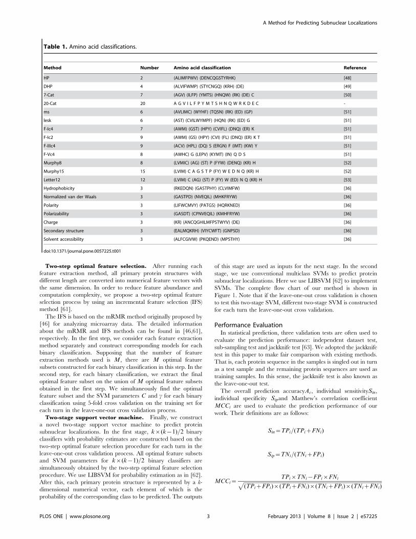
Table 1. Amino acid classifications.
Method Number Amino acid classification Reference
HP 2 (ALIMFPWV) (DENCQGSTYRHK) [48]
DHP 4 (ALVIFWMP) (STYCNGQ) (KRH) (DE) [49]
7-Cat 7 (AGV) (ILFP) (YMTS) (HNQW) (RK) (DE) C [50]
20-Cat 20 A G V I L F P Y M T S H N Q W R K D E C -
ms 6 (AVLIMC) (WYHF) (TQSN) (RK) (ED) (GP) [51]
lesk 6 (AST) (CVILWYMPF) (HQN) (RK) (ED) G [51]
F-Ic4 7 (AWM) (GST) (HPY) (CVIFL) (DNQ) (ER) K [51]
F-Ic2 9 (AWM) (GS) (HPY) (CVI) (FL) (DNQ) (ER) K T [51]
F-IIIc4 9 (ACV) (HPL) (DQ) S (ERGN) F (IMT) (KW) Y [51]
F-Vc4 8 (AWHC) G (LEPV) (KYMT) (IN) Q D S [51]
Murphy8 8 (LVMIC) (AG) (ST) P (FYW) (DENQ) (KR) H [52]
Murphy15 15 (LVIM) C A G S T P (FY) W E D N Q (KR) H [52]
Letter12 12 (LVIM) C (AG) (ST) P (FY) W (ED) N Q (KR) H [53]
Hydrophobicity 3 (RKEDQN) (GASTPHY) (CLVIMFW) [36]
Normalized van der Waals 3 (GASTPD) (NVEQIL) (MHKFRYW) [36]
Polarity 3 (LIFWCMVY) (PATGS) (HQRKNED) [36]
Polarizability 3 (GASDT) (CPNVEQIL) (KMHFRYW) [36]
Charge 3 (KR) (ANCQGHILMFPSTWYV) (DE) [36]
Secondary structure 3 (EALMQKRH) (VIYCWFT) (GNPSD) [36]
Solvent accessibility 3 (ALFCGIVW) (PKQEND) (MPSTHY) [36]
doi:10.1371/journal.pone.0057225.t001
A Method for Predicting Subnuclear Localizations
PLOS ONE | www.plosone.org 3 February 2013 | Volume 8 | Issue 2 | e57225

Ac~
Pi TPi
N, i~1,2,3, . . . ,k
where true positives TP=number of positive events that are
correctly predicted; true negatives TN=number of negative events
that are correctly predicted; false positives FP=number of
negative events that are incorrectly predicted to be positive; false
negatives FN=number of subjects that are predicted to be
negative despite they are positive; k=number of classes.
To further evaluate the performance of our method, we also use
the receiver operating characteristic (ROC) curve [64], which is
probably one of the most robust approaches for classifier
evaluation. The ROC curve is obtained by plotting true positive
rate (Sin) on the y-axis against the false positive rate (1{Sip) on the
x-axis. The area under the ROC curve (AUC) [65] can be used as
a reliable measure for the prediction performance. The case that
maximum value of AUC equals to 1 means a perfect prediction. A
random guess receives an AUC value close to 0.5.
Comparison of Feature Extraction Methods: Grid Searchvs Automatic SearchFirst, we observed each feature extraction method separately to
see which method is more effective. The same leave-one-out cross
validation process as [1] is used to evaluate each feature extraction
method and their combinations on Lei benchmark dataset. For
details, during the training process, each protein is selected as the
test sample in turn and the remaining ones constitute the training
set. We used a grid search approach to find optimal feature subsets
and optimize the SVM parameter C using 5-fold cross validation
on the training set for all binary classification models. For the
SVM parameter c, we use two kinds of methods to find the
optimal value: grid search and GFO [59]. It is found that the
number of elements of the optimal feature subset for each binary
classification is generally less than 300. So we chose the top-rank
300 features as the upper bound for optimal feature subset search.
The top-rank 10 features are used as an initial feature subset. The
size of the feature subset is increased by 10, obtaining 10, 20, 30,...,
300 features. At each size, we searched a pair (C,c) with the best 5-
fold cross validation (e.g. logC =25, 23, 21,..., 15; log c=215,
213, 211,..., 3). From this process, each binary classification
Table 2. 30 physicochemical properties of amino acids selected from AAindex database.
AAindex Physicochemical property Range of property
BULH740101 Transfer free energy to surface [22.46 0.16]
BULH740102 Apparent partial specific volume [0.558 0.842]
PONP800106 Surrounding hydrophobicity in turn [10.53 13.86]
PONP800104 Surrounding hydrophobicity in alpha-helix [10.98 14.08]
PONP800105 Surrounding hydrophobicity in beta-sheet [11.79 16.49]
PONP800106 Surrounding hydrophobicity in turn [9.93 15.00]
MANP780101 Average surrounding hydrophobicity [11.36 15.71]
EISD840101 Consensus normalized hydrophobicity scale [21.76 0.73]
JOND750101 Hydrophobicity [0.00 3.15]
HOPT810101 Hydrophilicity value [23.4 3.00]
PARJ860101 HPLC parameter [210.00 10.00]
JANJ780101 Average accessible surface area [22.8 103.0]
PONP800107 Accessibility reduction ratio [2.12 7.69]
CHOC760102 Residue accessible surface area in folded protein [18 97]
ROSG850101 Mean area buried on transfer [62.9 224.6]
ROSG850102 Mean fractional area loss [0.52 0.91]
BHAR880101 Average flexibility indices [0.295 0.544]
KARP850101 Flexibility parameter for no rigid neighbors [0.925 1.169]
KARP850102 Flexibility parameter for one rigid neighbor [0.862 1.085]
KARP850103 Flexibility parameter for two rigid neighbors [0.803 1.057]
JANJ780102 Percentage of buried residues [3 74]
JANJ780103 Percentage of exposed residues [5 85]
LEVM780101 Normalized frequency of alpha-helix, with weights [0.90 1.47]
LEVM780102 Normalized frequency of beta-sheet, with weights [0.72 1.49]
LEVM780103 Normalized frequency of reverse turn, with weights [0.41 1.91]
GRAR740102 Polarity [4.9 13.0]
GRAR740103 Volume [3 170]
MCMT640101 Refractivity [0.00 42.35]
PONP800108 Average number of surrounding residues [4.88 7.86]
KYTJ820101 Hydropathy index [24.5 4.5]
doi:10.1371/journal.pone.0057225.t002
A Method for Predicting Subnuclear Localizations
PLOS ONE | www.plosone.org 4 February 2013 | Volume 8 | Issue 2 | e57225

model corresponds to an optimal feature subset and a parameter
pair (C,c). Thus we can construct all binary classification models
and make preparation for training the second stage model. The
training method for the second stage model is identical to the first
stage except that it does not need feature selection. The final
prediction system was constructed as follows: the entire Lei dataset
of proteins is used as a training set; the optimal feature subsets for
each binary classification are taken as the union of all optimal
feature subsets obtained from the leave-one-out cross validation;
and the optimal value for each parameter of the SVMs for the
training set was taken as the average value of the optimal
parameters obtained from the leave-one-out cross validation. And
then the final system is tested on the multi-localization dataset and
the new independent testing set. Note that all parameters of the
final system including optimal features and SVM parameters are
not re-paramiterized to apply on the independent datasets.
The overall prediction accuracies for all feature extraction
methods on Lei data set and the new independent dataset are
listed in Table 3. We also combined the feature extraction
methods LAAC, LDC, GD, LZC, AD, SD and AC as one
method, named Combination1, in order to balance the number of
features used in the methods. In the following, the values on the
new independent dataset are shown in the parentheses From
Table 3, as far as the individual feature extraction method is
concerned, broadly speaking, the HHT method is the best. Its
prediction accuracy is 63.49% (65.87%), only worse than the
accuracy of 69.84% (70.83%) for Combination1. Of particular
interest, HHT outperforms DWT (57.54 and 56.15%), implying
that HHT is more effective. Note that HHT and DWT are both
time-frequency analysis methods and use similar definitions of
statistical features. Finally, we evaluate the performance of the
combination of all feature extraction methods, named Combina-
tion2. As shown in Table 3, Combination2 achieves the overall
accuracy of 77.8% (75.2%) for single-localization proteins, with
accuracy increase against individual methods between 7.9%
(4.4%) and 24.2% (22.2%).
We can also see from Table 3 that it takes far less CPU time to
train the models using GFO comparison with those using grid
search. Note that all experiments on the same PC (CPU: Intel
Core2 Duo T7700, 2.4 GHz; RAM: 3 GB). In view of this reason,
we propose the model using GFO as the system model although its
OAs are 2.6% lower than that using grid search.
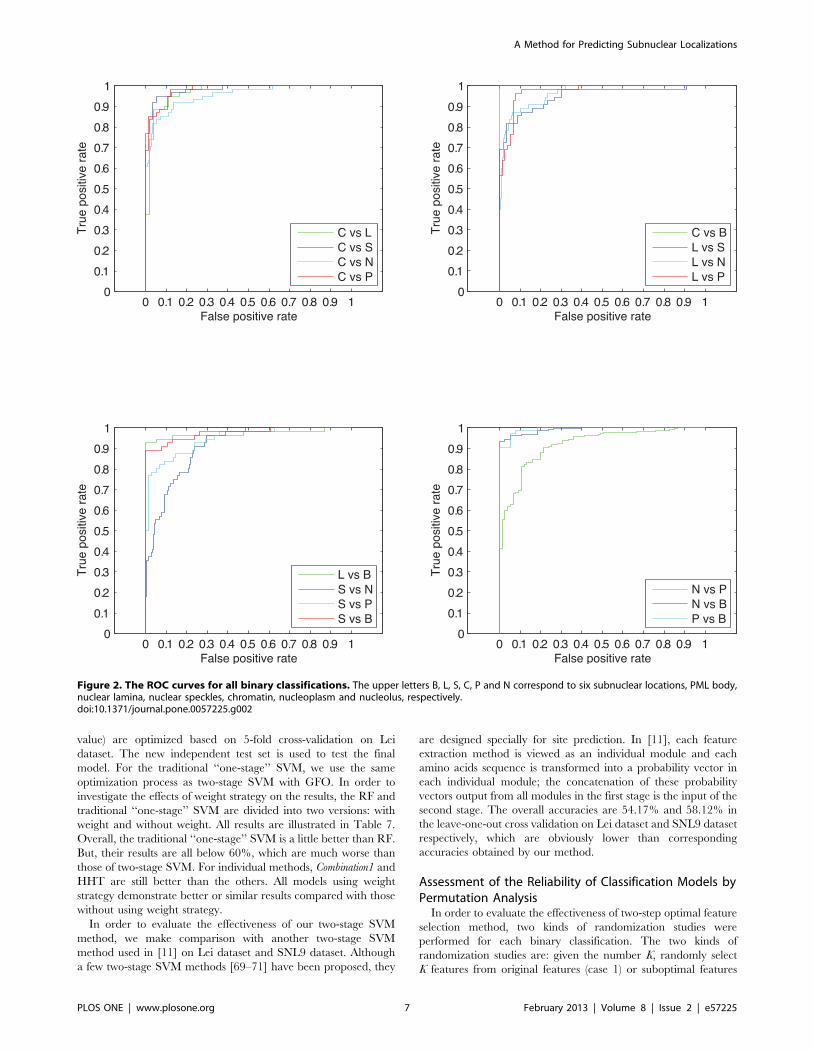
In addition, we also plot the ROC curves for each binary
classification in the final prediction system. The ROC curves are
shown in Figure 2. All the AUC values for these curves are over
0.9, which indicates that our predictions are satisfactory for all
binary classifications. One can see the binary classification for
Figure 1. The architecture of our method.doi:10.1371/journal.pone.0057225.g001
A Method for Predicting Subnuclear Localizations
PLOS ONE | www.plosone.org 5 February 2013 | Volume 8 | Issue 2 | e57225

nuclear speckles and nucleolus is the worst one, which degrades
the system performance.
Comparison with the Existing MethodsA comparison of the performance of our method (Combination2 )
against other existing methods on Lei dataset is illustrated in
Table 4, where better results are highlighted in bold. It is seen that
Combination2 achieves an overall accuracy of 77.8% (75.2%) for
single-localization proteins against 50.0% of SVM Ensemble [1],
against 66.5% of the GO-AA [21]. The measures Sn, Sp and MCC
reveal that Combination2 is far better than SVM Ensemble on all
subnuclear localizations, better than GO-AA on most subnuclear
localizations except Nuclear Speckles and Nuclear Lamina. Note that
SVM Ensemble and GO-AA did not give the results on the
measure Sp. The measures Sn, Sp and MCC reveal that
Combination2 is better than SpectrumKernel on most subnuclear
localizations except Nuclear Speckles and Nucleolus.
In order to make fair and reasonable comparison with the
SpectrumKernel method [2], we test our method using 5-fold cross
validation on Lei dataset. Its accuracies are 79.0% and 77.6%,
which are both obviously higher than 71.2% of the Spectrum-
Kernel method.
As shown in Table 4, Combination2 achieves better performance
on most small-size subnuclear localizations except Nuclear Speckles.
The performance of our method on large-size subnuclear
localizations Nucleolus is worse than SpectrumKernel; however it
also achieves 93.6% (91.3%) for Sn, which outperforms SVM
Ensemble (76.7%) and GO-AA (79.0%). Overall, the results show
that our method has good generalization abilities in predicting
subnuclear localizations regardless of the size of subnuclear
localizations.
In order to evaluate the performance of our method for multi-
localization proteins, we use the same criterion as in [1,21,66]. For
a protein with multi-localization, if one of the locations is predicted
true, then the entire prediction is considered correct. For the
independent set of multi-localization proteins, the overall accuracy
of Combination2 is 76.1% (71.7%), 11.1% (6.7) higher than SVM
Ensemble [1] and GO-AA [21]. The result reveals that
a combination of feature extraction methods integrates more
effectively information of the protein sequence to increase the
prediction accuracy.
Furthermore, comparing with GO-AA, our method only uses
information on amino acids of the protein sequence, and do not
use non-sequence information such as GO annotation, evolution-
ary information (e.g. PSI-BLAST profile), protein-protein in-
teraction and so on, which makes our method more general since
the PSI-BLAST profile is difficult to obtain and GO annotation
and protein-protein interaction may be missing for some proteins.
In addition, SpectrumKernel is based on kernel fusion, which is
computationally more intensive than sequence-based methods and
is also time consuming for training on a novel query sequence.
Furthermore, in order to make fair and reasonable comparison
with Nuc-Ploc [26], we test our method using leave-one-out cross
validation on SNL9 dataset. A web-server was designed in Nuc-
Ploc [26] by fusing PseAA composition and PsePSSM. The
detailed comparison results between our method and Nuc-Ploc are
listed in Table 5. As shown in Table 5, the overall accuracy of
prediction for 9 localizations is 72.1% in the leave-one-out cross
validation on SNL9 dataset, which is about 4.7% higher than the
overall accuracy obtained by Nuc-Ploc [26]. All MCCs of our
method are higher than Nuc-Ploc except for heterochromatin.
Analysis of Feature ContributionIn order to observe the contribution of the individual feature
extraction method to the overall prediction accuracy, we test some
possible combinations of feature extraction methods. Here, we
only report the second best combination for models using grid
search and GFO, respectively. For grid search, Combina-
tion1+HHT+DWT+PPDD is the second best combination, whose
OA are 75.00% and 64.6% on Lei dataset and the new
independent dataset. For GFO, Combination1+HHT +PPDD is
the second best combination, whose OA are 72.02% and 64.0%
on Lei dataset and the new independent dataset.
Moreover, the paired t-test is applied to the MCC values of
Combination2 and other individual methods to evaluate their
differences on the new independent dataset. The resulting P-
values are reported in Table 6. We can see that the P-values are
smaller than 0.05 for all individual methods, indicating that
Combination2 has made statistically significant improvements over
any other individual method for the subnuclear localization
prediction.
Comparison with Other Popular ClassifiersWe will also compare our two-stage SVM with Random Forest
(RF) classifier [67] as well as traditional ‘‘one-stage’’ SVM [62].
RF consists of a number of unpruned decision trees and is widely
used for classification and regression, especially for so-called "small
n, large p" problems [67]. It has two advantages: interpretable
classification rules and measure information about the importance
of features. Here, we use a Matlab package for implementing the
RF algorithm [68]. Two parameters, number of trees to grow ntree
and number of variables randomly sampled as candidates at each
split mtry are optimized using a grid search approach. During the
grid search, the values of ntree = 500:500:2000 and mtry= (default
Table 3. Comparison of the overall prediction accuracy between different feature extraction methods.
Feature extraction method Grid search GFO
Ac(%) CPU time (hr) Ac(%) CPU time (hr)
Combination1 69.84 (59.76) 2.704 70.83 (62.50) 0.406
RQA 53.57 (45.12) 2.174 52.98 (44.82) 0.413
HHT 63.49 (60.37) 2.336 65.87 (64.63) 0.427
PPDD 56.55 (53.35) 2.213 58.53 (59.15) 0.414
DWT 57.54(52.74) 2.035 56.15 (50.91) 0.402
Combination2 77.78 (70.12) 11.056 75.20 (69.82) 2.303
Note: the values on the new independent dataset are shown in the parentheses.doi:10.1371/journal.pone.0057225.t003
A Method for Predicting Subnuclear Localizations
PLOS ONE | www.plosone.org 6 February 2013 | Volume 8 | Issue 2 | e57225
value) are optimized based on 5-fold cross-validation on Lei
dataset. The new independent test set is used to test the final
model. For the traditional ‘‘one-stage’’ SVM, we use the same
optimization process as two-stage SVM with GFO. In order to
investigate the effects of weight strategy on the results, the RF and
traditional ‘‘one-stage’’ SVM are divided into two versions: with
weight and without weight. All results are illustrated in Table 7.
Overall, the traditional ‘‘one-stage’’ SVM is a little better than RF.
But, their results are all below 60%, which are much worse than
those of two-stage SVM. For individual methods, Combination1 and
HHT are still better than the others. All models using weight
strategy demonstrate better or similar results compared with those
without using weight strategy.
In order to evaluate the effectiveness of our two-stage SVM
method, we make comparison with another two-stage SVM
method used in [11] on Lei dataset and SNL9 dataset. Although
a few two-stage SVM methods [69–71] have been proposed, they
are designed specially for site prediction. In [11], each feature
extraction method is viewed as an individual module and each
amino acids sequence is transformed into a probability vector in
each individual module; the concatenation of these probability
vectors output from all modules in the first stage is the input of the
second stage. The overall accuracies are 54.17% and 58.12% in
the leave-one-out cross validation on Lei dataset and SNL9 dataset
respectively, which are obviously lower than corresponding
accuracies obtained by our method.
Assessment of the Reliability of Classification Models byPermutation AnalysisIn order to evaluate the effectiveness of two-step optimal feature
selection method, two kinds of randomization studies were
performed for each binary classification. The two kinds of
randomization studies are: given the number K, randomly select
K features from original features (case 1) or suboptimal features
Figure 2. The ROC curves for all binary classifications. The upper letters B, L, S, C, P and N correspond to six subnuclear locations, PML body,nuclear lamina, nuclear speckles, chromatin, nucleoplasm and nucleolus, respectively.doi:10.1371/journal.pone.0057225.g002
A Method for Predicting Subnuclear Localizations
PLOS ONE | www.plosone.org 7 February 2013 | Volume 8 | Issue 2 | e57225

(case 2) of the samples from two different subnuclear locations,
while keeping the class memberships unchanged. Then the newly
generated feature set is analyzed by using the same five-fold cross
validation as applied before to the original feature set. Here, the
given numbers of features K are set as one forth, half or all of the
number of optimal features. This procedure for case 1 is carried
out 50 rounds and the error rates (6standard deviation) over 50
permutations are shown in Figures 3, and compared with the
minimum error rates obtained from optimal features. For case 2,
similar results are obtained. In each case, the estimated error rate
obtained by optimal features is significantly lower than that
obtained by the randomization study. Especially, the misclassifi-
cation error rates obtained by using features selected randomly
from suboptimal features are also much lower than that estimated
by using those from the original features. If we do these two
randomization analysis on the whole original feature set 50 times,
overall error rates on average are 63.6% (64.6%) and 45.5%
(62.4%), which are both significantly higher than the error rate
21.2% obtained by optimal features. Therefore, it can be
concluded that two-step optimal feature selection method is
effective and reliable.
Since the relatively small sample size of some subdatasets in the
benchmark dataset, it is also important to evaluate the stability and
reliability of our classification model. In this paper, permutation
tests [72,73] are performed to compare the misclassification error
rates using our model with those from the randomization studies.
Initially, the class memberships of all the samples were permuted
while keeping features unchanged; then the newly generated
random dataset is analyzed by using the same cross validation
procedure applied before to the original dataset (SVM parameters
are the same as those chosen to obtain the minimum error rates for
original datasets). This procedure is also carried out 50 times and
the error rates (6standard deviation) over 50 permutations for all
binary classifications are shown in Figure 4 and compared with the
minimum error rates obtained from original datasets. As one can
Table 4. Performance comparison on Lei’s benchmark data set.
Subnuclear localization size
SVMensemble [1] Go-AA [21] SpectrumKernel [2]
Ourmethod
Sn MCC Sn MCC Sp Sn MCC Sp Sn MCC
PML Body 38 29.0 0.172 34.2 0.253 11.1 10.5 0.046 86.1(85.3)
55.3 (52.6) 0.298(0.273)
Nuclear Lamina 55 43.6 0.338 63.6 0.578 51.9 50.9 0.461 91.0 (91.9) 69.1 (70.9) 0.534(0.572)
Nuclear Speckles 56 35.7 0.363 62.5 0.607 86.7 69.6 0.754 91.8 (91.1) 62.5 (53.6) 0.503(0.460)
Chromatin 61 19.7 0.260 60.7 0.518 64.3 59.0 0.570 93.1(93.1)
73.8 (65.6) 0.640(0.572)
Nucleoplasm 75 22.7 0.206 56.0 0.504 52.6 54.7 0.465 90.8 (89.2) 64.0 (66.7) 0.526(0.520)
Nucleolus 219 76.7 0.367 79.0 0.656 89.8 96.4 0.880 78.6 (75.9) 93.6 (91.3) 0.726(0.570)
OA for single-localization 50.0 66.5 71.2 77.8(75.2)
OA for multi-localization 65.2 65.2 - 76.1(71.7)
Note: the values about models using GFO are shown in the parentheses.doi:10.1371/journal.pone.0057225.t004
Table 5. Performance comparison on SNL9 benchmark dataset.
Subnuclearlocalization Size MCC
Nuc-Ploc Our method
Chromatin 99 0.60 0.64
Heterochromatin 22 0.52 0.27
Nuclear envelope 61 0.53 0.58
Nuclear matrix 29 0.52 0.56
Nuclear porecomplex
79 0.70 0.70
Nuclear speckle 67 0.43 0.62
Nucleolus 307 0.57 0.69
Nucleoplasm 37 0.31 0.55
Nuclear PML body 13 0.32 0.43
Ac(%) 67.4% 72.1%
Note: MCCs and Ac about Nuc-Ploc are obtained directly from the originalpaper [26].doi:10.1371/journal.pone.0057225.t005
Table 6. Comparisons of Combination2 with the individualmethod on the new independent dataset.
Methods Grid search GFO
P-values P-values
Combination1 0.022 0.028
RQA 4.461e24 3.494e24
HHT 0.037 0.025
PPDD 0.005 0.004
DWT 0.003 0.001
doi:10.1371/journal.pone.0057225.t006
A Method for Predicting Subnuclear Localizations
PLOS ONE | www.plosone.org 8 February 2013 | Volume 8 | Issue 2 | e57225

see, the estimated error rates obtained by our method for original
dataset are significantly lower than those from the randomization
studies. If we do the same permutation test on the whole original
dataset, overall error rate on average is 76.7% (66.1%), which is
much higher than the error rate 21.2% obtained by using optimal
features. In summary, classification information can be character-
ized by optimal features; otherwise, the estimated error rate
obtained from original dataset will be close to that calculated from
the shuffled dataset.
ConclusionsIn this section, we will summarize our conclusions as follows.
1. From the results on three datasets, our ensemble method is
effective and valuable for predicting protein subnuclear
localizations compared with existing methods for the same
problem.
2. From contribution of features as shown in Table 3 and 6,
Combination1 and HHT make the most important contribu-
tion, DWT and PPDD the second, and RQA is worst.
3. The method GFO can effectively find the optimal RBF kernel
parameter and further speed up our method.
4. This problem cannot be solved by simply using popular
machine learning classifiers (such as SVM, RF).
5. The weight strategy is important for this problem (unbalanced
dataset).
6. Two-step optimal feature selection method is effective.
7. Effective classification for nuclear speckles and nucleolus is the
key factor.
Although our method obtain relatively satisfactory results, some
open problems need to be investigated in the future. Subnuclear
localization prediction can be considered multi-label, unbalanced
problem. Hence, popular methods for multi-label, unbalanced
problems may be applied to improve this work.
Table 7. Comparisons with other popular classifiers on thenew independent dataset.
Methods
TraditionalSVM (Ac(%))
RandomForest (Ac(%))
weightwithoutweight weight without weight
Combination1 59.45 57.62 58.54 57.32
RQA 45.73 45.73 45.73 44.82
HHT 59.76 56.10 57.93 56.10
PPDD 58.54 57.93 55.49 55.18
DWT 57.62 55.49 52.74 51.52
Combination2 66.16 64.63 64.02 63.11
doi:10.1371/journal.pone.0057225.t007
Figure 3. Comparisons of error rate (percentage of misclassified samples) over 50 runs of randomization analysis. Random 1:selecting randomly features subsets from original features, whose size is one-forth of the number of optimal features; Random 2: one half of thenumber of optimal features; Random 3: equal to the number of optimal features.doi:10.1371/journal.pone.0057225.g003
A Method for Predicting Subnuclear Localizations
PLOS ONE | www.plosone.org 9 February 2013 | Volume 8 | Issue 2 | e57225

Methods
Feature Extraction Methods Based on Amino AcidClassificationSuppose that 20 amino acids are divided into n groups, denoted
by A, according to certain classification method listed in Table 1.
Then, for a given protein sequence S of length N, we may obtain
a new sequence S0of n symbols with the same length as S, each
symbol corresponding to one group of amino acids.
Local amino acid composition (LAAC) and local dipeptide
composition (LDC). Protein targeting signals are fragments of
amino acid sequences, usually on N-terminal or C-terminal,
responsible for directing proteins to their target locations. They are
usually located at the N-terminal or C-terminal of a protein
sequence [74]. But they are difficult to detect and define signal
motifs. Here we compute local amino acid composition and local
dipeptide composition on the first 60 amino acids from the N-
terminal and 15 amino acids from the C-terminal of a protein
sequence to represent protein targeting signals, which is inspired
by [11]. Finally, 2|(nzn2) features are generated.
Global descriptor (GD). The global descriptor method was
proposed first by [34] for predicting protein folding classes and
later applied to predict human Pol II promoter sequences [75] and
distinguish coding from non-coding sequences in a prokaryote
complete genome [76] by our group. The global descriptor
contains three parts: composition (Comp), transition (Tran) and
distribution (Dist). Comp describes the overall composition of a given
symbol in the new symbol sequence. Tran characterizes the
percentage frequency that amino acids of a particular symbol are
followed by a different one. Dist measures the chain length within
which the first, 25, 50, 75 and 100% of the amino acids of
a particular symbol are located [34]. Overall, we get
6|nzn|(n{1)=2 features from the global descriptor for S0.
Lempel-Ziv complexity (LZC). The Lempel-Ziv (LZ) com-
plexity is one of the conditional complexity measures of symbol
sequences. It can reflect most adequately the repeated patterns
occurring in the symbol sequence and are also easily computed
[35]. The LZ complexity has been successfully employed to
construct phylogenetic tree [77] and predict protein structural
class [78]. Let S0
i:j be the subsequence of S0between position i and
j. The LZ complexity of sequence S0, usually denoted by c(S
0), is
defined as the minimal number of steps with which S0 is
synthesized from null sequence according to the rule that at each
step only two operations are allowed: either copying the longest
fragment from the part of S0that has already been synthesized or
generating an additional symbol. Suppose that the sequence S0is
decomposed into.
S0~S
01:i1
S0i1z1:i2
� � �S0ikz1:N
This decomposition is also called the exhaustive history of S0,
denoted by H(S0). It is proved that every sequence has a unique
exhaustive history [35]. For example, for the sequence , its
exhaustive history is H(S)~A:E:F :FG:EFFGA:E, where ‘‘:’’ is
used to separate the decomposition components. So, c(S0)=6.
Figure 4. Comparisons of error rate (percentage of misclassified samples) over 50 runs of permutation analysis. The original classmemberships of all samples are randomly shuffled for 50 times and then used together with original optimal features for classification using the samecross validation as applied before for original dataset.doi:10.1371/journal.pone.0057225.g004
A Method for Predicting Subnuclear Localizations
PLOS ONE | www.plosone.org 10 February 2013 | Volume 8 | Issue 2 | e57225

Feature Extraction Methods Based on PhysicochemicalProperties
Autocorrelation descriptors (AD). Three widely-used au-
tocorrelation descriptors are selected: normalized Moreau-Broto
autocorrelation descriptors, Moran autocorrelation descriptors
and Geary autocorrelation descriptors [36]. They are all defined
based on the value distributions of 30 physicochemical properties
of amino acids along a protein sequence (see Table 2). The
measurement values of these properties are first standardized to
have zero mean and unit standard deviation and then the three
autocorrelation descriptors are calculated. These descriptors are
also used for the classification of G-protein-coupled receptors by
Peng et al. [79].
The normalized Moreau-Broto autocorrelation descriptors are defined
as.
NMBA(l)~NBA(l)
N{l,l~1,2, � � � ,30,
where MBA(l)~PN{l
i~1
P(AAi)P(AAizl), AAi and AAizl are the
amino acids at position i and izl along the protein sequence,
respectively. P(AAi) and P(AAizl) are standardized property
values of amino acid AAiand AAizl , respectively. The maximum
value of l is set at 30 as in [36].
The Moran autocorrelation descriptors are defined as.
MA(l)~
1N{l
PN{l
i~1
(P(AAi){~PP)(P(AAizl){~PP)
1N
PNi~1
(P(AAi){~PP)2, l~1,2, � � � ,30,
where ~PP is the mean value of the property under consideration
along the sequence.
The Geary autocorrelation descriptors are defined as.
GA(l)~
12(N{l)
PN{l
i~1
(P(AAi){P(AAizl))2
1N
PNi~1
(P(AAi){~PP)2, l~1,2, � � � ,30,
For each AD, we obtain 900 ( = 30630) features. In total, 2700
( = 90063) features are obtained to describe a protein sequence.
Sequence-order descriptors (SD). In order to derive the
sequence-order descriptors, we use two distance matrices for
amino acid pairs. One is called the Grantham chemical distance matrix
[36], and the other is called the Schneider-Wrede physicochemical
distance matrix [37]. Then, the jth-rank sequence-order coupling number is
defined as.
t(l)~XN{l
i~1
(d(AAi,AAizl))2, l~1,2, � � � ,30
where is d(AAi,AAizl) one of the above two distances between
two amino acids AAi and AAizl located at position i and position
izl, respectively.
The quasi-sequence-order descriptors are defined as.
QSO(i)~
fA(i)P20i~1
fA(i)zvP30j~1
t(j)
, 1ƒiƒ20,
v:t(j)P20i~1
fA(i)zvP30j~1
t(j)
, 21ƒiƒ50,
8>>>>>><>>>>>>:
where fA(i) is the occurrence frequencies of 20 amino acids in
a protein sequence and v is a weighting factor (with default
v=0.1).
We end up with 60 ( = 3062) sequence-order-coupling numbers
and 100 ( = 5062) quasi-sequence-order descriptors. In total, there
are 160 features extracted from SD.
Auto covariance (AC). The autocovariance method is
a statistical tool proposed by Wold et al. [38] which can capture
local sequence-order information. It has been applied to many
fields of bioinformatics, such as functional discrimination of
membrane proteins [39], predicting protein submitochondria
locations [40], and so on.
The autocovariance method is defined as.
ACD(l)~1
m{l
Xm{l
i~1
(P(AAi){~PP)(P(AAizl){~PP), l~1,2, � � � ,30:
The AC is computed on 531 physicochemical properties
mentioned earlier in Subsection Physicochemical properties.
Physicochemical property distribution descriptor
(PPDD). The physicochemical property distribution descriptor
is first proposed by [41] for remote homology detection. In this
descriptor, the protein sequence of length N is first transformed
from the 20 amino acid letter code to N-dimension numerical
vector associated with the index being used. The average across all
4-mers is taken to create a new N{3-dimensional numerical
vector. This new vector is then normalized to have the mean and
standard deviation of the theoretical values associated with the
index. This normalized numerical vector is transformed into
a discrete distribution of 18 frequency values, where each value
represents a range of 0.5, i.e., the first bin contains all values less
than24, the second bin contains all values between24 and23.5,
and so forth. So, for every physicochemical property, the
physicochemical property distribution descriptor generates 18
features.
Recurrence plot and recurrence quantification analysis
(RQA). Recurrence plot (RP) is a purely graphical tool originally
proposed by [80] to visualize patterns of recurrence in the data. A
time series x1,x2, . . . ,xNf g with length N can be embedded in the
space Rm with embedding dimension m and a time delay taccording to nonlinear dynamic theory [81]. Supposing that
~yyif gNm
1 represents a trajectory in the corresponding phase space,
we have.
~yyi~(xi,xizt,xiz2t, . . . ,xiz(m{1)t),i~1,2, . . . ,Nm,
where Nm~N{(m{1)t:Once a norm function has been selected
(e.g., the commonly chosen Euclidean norm [82]), we can
calculate the distance matrix (DM) from the above points Nm.
DM is an Nm|Nm square matrix whose elements are the
distances between any pair of points. DM can be transformed into
a rescaled distance matrix (RDM) through dividing each element
in the DM by the maximum value of DM [81]. After obtaining
A Method for Predicting Subnuclear Localizations
PLOS ONE | www.plosone.org 11 February 2013 | Volume 8 | Issue 2 | e57225
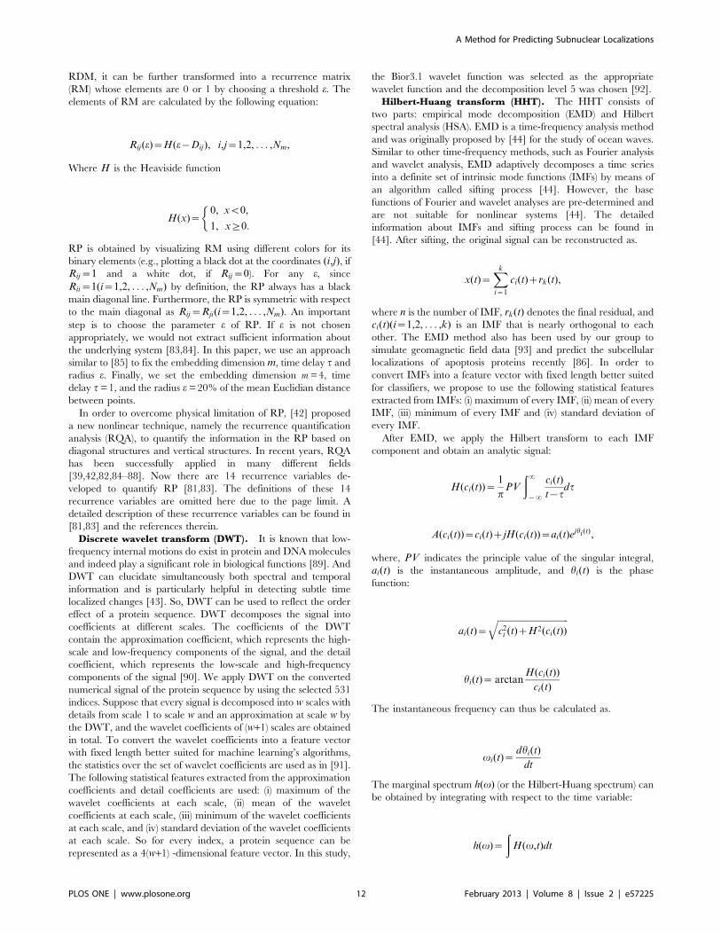
RDM, it can be further transformed into a recurrence matrix
(RM) whose elements are 0 or 1 by choosing a threshold e. Theelements of RM are calculated by the following equation:
Rij(e)~H(e{Dij), i,j~1,2, . . . ,Nm,
Where H is the Heaviside function
H(x)~0, xv0,
1, x§0:
�
RP is obtained by visualizing RM using different colors for its
binary elements (e.g., plotting a black dot at the coordinates (i,j), ifRij~1 and a white dot, if Rij~0). For any e, since
Rii~1(i~1,2, . . . ,Nm) by definition, the RP always has a black
main diagonal line. Furthermore, the RP is symmetric with respect
to the main diagonal as Rij~Rji(i~1,2, . . . ,Nm). An important
step is to choose the parameter e of RP. If e is not chosen
appropriately, we would not extract sufficient information about
the underlying system [83,84]. In this paper, we use an approach
similar to [85] to fix the embedding dimension m, time delay t andradius e. Finally, we set the embedding dimension m= 4, time
delay t= 1, and the radius e= 20% of the mean Euclidian distance
between points.
In order to overcome physical limitation of RP, [42] proposed
a new nonlinear technique, namely the recurrence quantification
analysis (RQA), to quantify the information in the RP based on
diagonal structures and vertical structures. In recent years, RQA
has been successfully applied in many different fields
[39,42,82,84–88]. Now there are 14 recurrence variables de-
veloped to quantify RP [81,83]. The definitions of these 14
recurrence variables are omitted here due to the page limit. A
detailed description of these recurrence variables can be found in
[81,83] and the references therein.
Discrete wavelet transform (DWT). It is known that low-
frequency internal motions do exist in protein and DNA molecules
and indeed play a significant role in biological functions [89]. And
DWT can elucidate simultaneously both spectral and temporal
information and is particularly helpful in detecting subtle time
localized changes [43]. So, DWT can be used to reflect the order
effect of a protein sequence. DWT decomposes the signal into
coefficients at different scales. The coefficients of the DWT
contain the approximation coefficient, which represents the high-
scale and low-frequency components of the signal, and the detail
coefficient, which represents the low-scale and high-frequency
components of the signal [90]. We apply DWT on the converted
numerical signal of the protein sequence by using the selected 531
indices. Suppose that every signal is decomposed into w scales with
details from scale 1 to scale w and an approximation at scale w by
the DWT, and the wavelet coefficients of (w+1) scales are obtainedin total. To convert the wavelet coefficients into a feature vector
with fixed length better suited for machine learning’s algorithms,
the statistics over the set of wavelet coefficients are used as in [91].
The following statistical features extracted from the approximation
coefficients and detail coefficients are used: (i) maximum of the
wavelet coefficients at each scale, (ii) mean of the wavelet
coefficients at each scale, (iii) minimum of the wavelet coefficients
at each scale, and (iv) standard deviation of the wavelet coefficients
at each scale. So for every index, a protein sequence can be
represented as a 4(w+1) -dimensional feature vector. In this study,
the Bior3.1 wavelet function was selected as the appropriate
wavelet function and the decomposition level 5 was chosen [92].
Hilbert-Huang transform (HHT). The HHT consists of
two parts: empirical mode decomposition (EMD) and Hilbert
spectral analysis (HSA). EMD is a time-frequency analysis method
and was originally proposed by [44] for the study of ocean waves.
Similar to other time-frequency methods, such as Fourier analysis
and wavelet analysis, EMD adaptively decomposes a time series
into a definite set of intrinsic mode functions (IMFs) by means of
an algorithm called sifting process [44]. However, the base
functions of Fourier and wavelet analyses are pre-determined and
are not suitable for nonlinear systems [44]. The detailed
information about IMFs and sifting process can be found in
[44]. After sifting, the original signal can be reconstructed as.
x(t)~Xki~1
ci(t)zrk(t),
where n is the number of IMF, rk(t) denotes the final residual, andci(t)(i~1,2, . . . ,k) is an IMF that is nearly orthogonal to each
other. The EMD method also has been used by our group to
simulate geomagnetic field data [93] and predict the subcellular
localizations of apoptosis proteins recently [86]. In order to
convert IMFs into a feature vector with fixed length better suited
for classifiers, we propose to use the following statistical features
extracted from IMFs: (i) maximum of every IMF, (ii) mean of every
IMF, (iii) minimum of every IMF and (iv) standard deviation of
every IMF.
After EMD, we apply the Hilbert transform to each IMF
component and obtain an analytic signal:
H(ci(t))~1
pPV
ð?{?
ci(t)
t{tdt
A(ci(t))~ci(t)zjH(ci(t))~ai(t)ejhi (t),
where, PV indicates the principle value of the singular integral,
ai(t) is the instantaneous amplitude, and hi(t) is the phase
function:
ai(t)~
ffiffiffiffiffiffiffiffiffiffiffiffiffiffiffiffiffiffiffiffiffiffiffiffiffiffiffiffiffiffiffiffic2i (t)zH2(ci(t))
q
hi(t)~ arctanH(ci(t))
ci(t)
The instantaneous frequency can thus be calculated as.
vi(t)~dhi(t)
dt
The marginal spectrum h(v) (or the Hilbert-Huang spectrum) can
be obtained by integrating with respect to the time variable:
h(v)~
ðH(v,t)dt
A Method for Predicting Subnuclear Localizations
PLOS ONE | www.plosone.org 12 February 2013 | Volume 8 | Issue 2 | e57225

The marginal spectrum offers a measure of total amplitude
contribution from each frequency.If the Hilbert-Huang spectrum
is denoted as a function of frequency f instead of angle frequency
v, the marginal spectrum can be calculated for each IMF and then
normalized by.
hh(f )~h(f )Pf
h(f ):
(c.f. [45]). Then, applying the Shannon entropy theory to the
normalized marginal spectrum, the Hilbert-Huang spectral
entropy (HHSE) is obtained as.
H~{Xf
hh(f ) log (hh(f )),
HHSE~H=log (N),
where N is the number of frequency components and the value of
HHSE varies between 0 (complete regularity) and 1 (maximum
irregularity).
For each physicochemical property index selected, 4|kz1features are obtained in total in HHT.
Acknowledgments
The authors would like to thank A/Prof. Jian-Mei Yuan in Xiangtan
University for her help on the web server development.
Author Contributions
Conceived and designed the experiments: GSH ZYG. Performed the
experiments: GSH. Analyzed the data: GSH ZYG VA. Contributed
reagents/materials/analysis tools: GSH ZYG APDK YCT. Wrote the
paper: GSH ZYG VA YCT.
References
1. Lei ZD, Dai Y (2005) An SVM-based system for predicting protein subnuclear
localizations. BMC Bioinformatics 6: 291.
2. Mei SY, Fei W (2010) Amino acid classification based spectrum kernel fusion for
protein subnuclear localization. BMC Bioinformatics (Suppl 1): S17.
3. Shen HB, Chou KC (2005) Predicting protein subnuclear location with
optimized evidence-theoretic K-nearest classifier and pseudo amino acid
composition. Biochem Biophys Res Commun 337: 752–756.
4. Phair RD, Misteli T (2000) High mobility of proteins in the mammalian cell
nucleus. Nature 404: 604–609.
5. Murphy RF, Boland MV, Velliste M (2000) Towards a systematics for protein
subcellular location: quantitative description of protein localization patterns and
automated analysis of fluorescence microscope images. Proc Int Conf Intell Syst
Mol Biol 8: 251–259.
6. Briesemeister S, RahnenfAuhrer J, Kohlbacher O (2010) Going from where to
why-interpretable prediction of protein subcellular localization. Bioinformatics
26: 1232–1238.
7. Cedano J, Aloy P, Perez-Pons JA, Querol E (1997) Relation between amino acid
composition and cellular location of proteins. J Mol Biol 266: 594–600.
8. Emanuelsson O, Nielsen H, Brunak S, von Heijne G (2000) Predicting
subcellular localization of proteins based on their N-terminal amino acid
sequence. J Mol Biol 300: 1005–1016.
9. Emanuelsson O, Brunak S, von Heijne G, Nielsen H (2007) Locating proteins in
the cell using TargetP, SignalP and related tools. Nat Protoc 2: 953–971.
10. Huang WL, Tung CW, Huang HL, Hwang SF, Ho SY (2007) ProLoc:
prediction of protein subnuclear localization using SVM with automatic
selection from physicochemical composition features. BioSystems 90: 573–581.
11. Hoglund A, Donnes P, Blum T, Adolph HW, Kohlbacher O (2006) MultiLoc:
prediction of protein subcellular localization using N-terminal targeting
sequences, sequence motifs and amino acid composition. Bioinformatics 22:
1158–1165.
12. Nakashima H, Nishikawa K (1994) Discrimination of intracellular and
extracellular proteins using amino acid composition and residue-pair frequen-
cies. J Mol Biol 238: 54–61.
13. Pierleoni A, Martelli PL, Fariselli P, Casadio R (2006) BaCelLo: a balanced
subcellular localization predictor. Bioinformatics 22: e408–416.
14. Sarda D, Chua GH, Li KB, Krishnan A (2005) pSLIP: SVM based protein
subcellular localization prediction using multiple physicochemical properties.
BMC Bioinformatics 6: 152.
15. Wang J, Sung WK, Krishnan A, Li KB (2005) Protein subcellular localization
prediction for Gram-negative bacteria using amino acid subalphabets and
a combination of multiple support vector machines. BMC Bioinformatics 6: 174.
16. Yu NY, Wagner JR, Laird MR, Melli G, Rey S, et al. (2010) PSORTb 3.0:
improved protein subcellular localization prediction with refined localization
subcategories and predictive capabilities for all prokaryotes. Bioinformatics 26:
1608–1615.
17. Zheng XQ, Liu TG, Wang J (2009) A complexity-based method for predicting
protein subcellular location. Amino Acids 37: 427–433.
18. Chou KC, Cai YD (2002) Using functional domain composition and support
vector machines for prediction of protein subcellular location. J Biol Chem 277:
45765–45769.
19. Chou KC, Cai YD (2004) Prediction of protein subcellular locations by GO-
FunD-PseAA predictor. Biochem Biophys Res Commun 320: 1236–1239.
20. Chou KC, Shen HB (2010) A New Method for Predicting the Subcellular
Localization of Eukaryotic Proteins with Both Single and Multiple Sites: Euk-mPLoc 2.0. PLoS One 5: e9931.
21. Lei ZD, Dai Y (2006) Assessing protein similarity with Gene Ontology and its
use in subnuclear localization prediction. BMC Bioinformatics 7: 491.
22. Mei SY, Fei W, Zhou SG (2011) Gene ontology based transfer learning for
protein subcellular localization. BMC Bioinformatics 12: 44.
23. Chang JM, Su EC, Lo A, Chiu HS, Sung TY, et al. (2008) PSLDoc: Proteinsubcellular localization prediction based on gapped-dipeptides and probabilistic
latent semantic analysis. Proteins 72: 693–710.
24. Guo J, Lin YL (2006) TSSub: eukaryotic protein subcellular localization byextracting features from profiles. Bioinformatics 22: 1784–1785.
25. Mundra P, Kumar M, Kumar KK, Jayaraman VK, Kulkarni BD (2007) Using
pseudo amino acid composition to predict protein subnuclear localization:Approached with PSSM. Pattern Recognit Lett 28: 1610–1615.
26. Shen HB, Chou KC (2007) Nuc-PLoc: a new web-server for predicting protein
subnuclear localization by fusing PseAA composition and PsePSSM. Protein EngDes Sel 20: 561–567.
27. Xiao RQ, Guo YZ, Zeng YH, Tan HF, Pu XM, et al. (2009) Using position
specific scoring matrix and autocovariance to predict protein subnuclearlocalization. J Bio Sci Eng 2: 51–56.
28. Shin CJ, Wong S, Davis MJ, Ragan MA (2009) Protein-protein interaction as
a predictor of subcellular location. BMC Syst Biol 3: 28.
29. Guda C, Subramaniam S (2005) pTARGET: a new method for predicting
protein subcellular localization in eukaryotes. Bioinformatics 21: 3963–3969.
30. Shen HB, Chou KC (2009) A top-down approach to enhance the power ofpredicting human protein subcellular localization: Hum-mPLoc 2.0. Anal
Biochem 394: 269–274.
31. Carmo-Fonseca M (2002) The contribution of nuclear compartmentalization togene regulation. Cell 108: 513–521.
32. Hancock R (2004) Internal organisation of the nucleus: assembly of compart-
ments by macromolecular crowding and the nuclear matrix model. Biol Cell 96:595–601.
33. Sutherland HG, Mumford GK, Newton K, Ford LV, Farrall R, et al. (2001)
Large-scale identification of mammalian proteins localized to nuclear sub-compartments. Hum Mol Genet 10: 1995–2011.
34. Dubchak I, Muchnik I, Holbrook SR, Kim SH (1995) Prediction of protein
folding class using global description of amino acid sequence. Proc Natl AcadSci U S A 92: 8700–8704.
35. Lempel A, Ziv J (1976) On the complexity of finite sequence. IEEE Trans Inf
Theory 22: 75–81.
36. Li ZR, Lin HH, Han LY, Jiang L, Chen X, et al. (2008) PROFEAT: a web
server for computing structural and physicochemical features of proteins and
peptides from amino acid sequence. Nucleic Acids Res 34: W32–W37.
37. Chou KC (2000) Prediction of protein subcellular locations by incorporating
quasi-sequence-order effect. Biochem Biophys Res Commun 278: 477–483.
38. Wold S, Jonsson J, Sjostrom M, Sandberg M, Rannar S (1993) DNA andpeptide sequences and chemical processes multivariately modelled by principal
component analysis and partial least -squares projections to latent structures.Anal Chim Acta 277: 239–253.
39. Yang L, Li YZ, Xiao RQ, Zeng YH, Xiao JM, et al. (2010) Using auto
covariance method for functional discrimination of membrane proteins based onevolution information. Amino Acids 38: 1497–1503.
A Method for Predicting Subnuclear Localizations
PLOS ONE | www.plosone.org 13 February 2013 | Volume 8 | Issue 2 | e57225

40. Zeng YH, Guo YZ, Xiao RQ, Yang L, Yu LZ, et al. (2009) Using the
augmented Chou’s pseudo amino acid composition for predicting proteinsubmitochondria locations based on auto covariance approach. J Theor Biol
259: 366–372.
41. Webb-Robertson BJ, Ratuiste KG, Oehmen CS (2010) Physicochemicalproperty distributions for accurate and rapid pairwise protein homology
detection. BMC Bioinformatics 11: 145.42. Webber CL, Zbilut JP (1994) Dynamical assessment of physiological systems and
states using recurrence plot strategies. J Appl Physiol 76: 965–973.
43. Mori K, Kasashima N, Yoshioka T, Ueno Y (1996) Prediction of spalling ona ball bearing by applying the discrete wavelet transform to vibration signals.
Wear 195: 162–168.44. Huang NE, Shen Z, Long SR, Wu MC, Shih SH, et al. (1998) The empirical
mode decomposition and the Hilbert spectrum for nonlinear and nonstationarytime series analysis. Proc R Soc A 454: 903–995.
45. Shi F, Chen QJ, Li NN (2008) Hilbert Huang transform for predicting proteins
subcellular location. J Biomed Sci Eng 1: 59–63.46. Peng H, Long F, Ding C (2005) Feature selection based on mutual information:
criteria of max-dependency, max-relevance, and min-redundancy. IEEE TransPattern Anal Mach Intell 27: 1226–1238.
47. Dellaire G, Farrall R, Bickmore WA (2003) The Nuclear Protein Database
(NPD): subnuclear localisation and functional annotation of the nuclearproteome. Nucleic Acids Res 31: 328–330.
48. Dill KA (1985) Theory for the folding and stability of globular proteins.Biochemistry 24: 1501–1509.
49. Yu ZG, Anh V, Lau KS (2004) Fractal analysis of measure representation oflarge proteins based on the detailed HP model. Physica A 337: 171–184.
50. Shen J, Zhang J, Luo X, Zhu W, Yu K, et al. (2007) Predicting protein-protein
interactions based only on sequences information. Proc Natl Acad Sci U S A104: 4337–4341.
51. Sanchez-Flores A, Perez-Rueda E, Segovia L (2008) Protein homology detectionand fold inference through multiple alignment entropy profiles. Proteins 70:
248–256.
52. Murphy LR, Wallqvist A, Levy RM (2000) Simplified amino acid alphabets forprotein fold recognition and implications for folding. Protein Eng 13: 149–152.
53. Basu S, Pan A, Dutta C, Das J (1997) Chaos game representation of proteins.J Mol Graph Model 15: 279–289.
54. Kawashima S, Kanehisa M (2000) AAindex: amino acid index database. NucleicAcids Res 28: 374.
55. Bhasin M, Raghava GP (2004) ESLpred: SVM-based method for subcellular
localization of eukaryotic proteins using dipeptide composition and PSI-BLAST.Nucleic Acids Res 32: W414–419.
56. Vapnik VN (1995) The Nature of Statistical Learning Theory. Springer.57. Platt JC, Cristianini N, Shawe-Taylor J (2000) Large margin DAGs for
multiclass classification. Advances in Neural Information Processing Systems.
Cambridge: 547–553.58. Wang J, Lu HP, Plataniotis KN, Lu JW (2009) Gaussian kernel optimization for
pattern classification. Pattern Recognit 42: 1237–1247.59. Yin JB, Li T, Shen HB (2011) Gaussian kernel optimization: Complex problem
and a simple solution. Neurocomputing 74: 3816–3822.60. Blum T, Briesemeister S, Kohlbacher O (2009) MultiLoc2: integrating
phylogeny and Gene Ontology terms improves subcellular protein localization
prediction. BMC Bioinformatics 10: 274.61. Huang T, Shi XH, Wang P, He ZS, Feng KY, et al. (2010) Analysis and
Prediction of the Metabolic Stability of Proteins Based on Their SequentialFeatures, Subcellular Locations and Interaction Networks. PLoS One 5: e10972.
62. Chang CC, Lin CJ (2001) LIBSVM: a library for support vector machines.
Available: http://www.csie.ntu.edu.tw/cjlin/papers/libsvm.pdf.63. Chou KC (1995) A novel approach to predicting protein structural classes in
a (20–1)-D amino acid composition space. Proteins 21: 319–344.64. Swets JA (1988) Measuring the accuracy of diagnostic systems. Science 240:
1285–1293.
65. Bradley AP (1997) The use of the area under the ROC curve in the evaluation ofmachine learning algorithms. Pattern Recognit 30: 1145–1159.
66. Gardy JL, Laird MR, Chen F, Rey S,Walsh CJ, et al. (2005) PSORTb v.2.0:expanded prediction of bacterial protein subcellular localization and insights
gained from comparative proteome analysis. Bioinformatics 21: 617–623.67. Breman L (2001) Random forest. Machine Learning 45: 5–32.
68. randomforest-matlab. Available: http://code.google.com/p/randomforest-
matlab/.69. Nguyen MN, Rajapakse JC (2005) Prediction of protein relative solvent
accessibility with a two-stage SVM approach. Proteins 59: 30–37.
70. Nguyen MN, Rajapakse JC (2007) Prediction of Protein Secondary Structurewith two-stage multi-class SVMs. Int J Data Min Bioinform 1: 248–269.
71. Gubbi J, Shilton A, Parker M, Palaniswami M (2006) Protein topologyclassification using two-stage support vector machines. Genome Inform 17: 259–
269.
72. Nguyen DV, Rocke DM (2002) Tumor classification by partial least squaresusing microarray gene expression data. Bioinformatics 18: 39–50.
73. Tan YX, Shi LM, Tong WD, Wang C (2005) Multi-class cancer classification bytotal principal component regression (TPCR) using microarray gene expression
data. Nucleic Acids Res 33: 56–65.74. Silhavy TJ, Benson SA, Emr SD (1983) Mechanisms of Protein Localization.
Microbiol Rev 47: 313–344.
75. Yang JY, Zhou Y, Yu ZG, Anh V, Zhou LQ (2008) Human Pol II promoterrecognition based on primary sequences and free energy of dinucleotides. BMC
Bioinformatics 9: 11.76. Han GS, Yu ZG, Anh V, Chan RH (2009) Distinguishing coding from non-
coding sequences in a prokaryote complete genome based on the global
descriptor. Proceedings of The 6th International Conference on Fuzzy Systemsand Knownledge Discovery: 42–46.
77. Otu HH, Sayood K (2003) A new sequence distance measure for phylogenetictree construction. Bioinformatics 19: 2122–2130.
78. Liu TG, Zheng XQ, Wang J (2010) Prediction of protein structural class usinga complexity-based distance measure. Amino Acids 38: 721–728.
79. Peng ZL, Yang JY, Chen X (2010) An improved classification of G-protein-
coupled receptors using sequence-derived features. BMC Bioinformatics 11: 420.80. Eckmann JP, Kamphorst SO, Ruelle D (1987) Recurrence plots of dynamical
systems. Europhys Lett 4: 973–977.81. Riley MA, Van OGC (2005) Tutorials in contemporary nonlinear methods for
the behavioral sciences. Available: http://www.nsf.gov/sbe/bcs/pac/nmbs/
nmbs.jsp.82. Giuliani A, Benigni R, Zbilut JP, Webber CL, Sirabella P, et al. (2002)
Nonlinear signal analysis methods in the elucidation of protein sequence-structure relationships. Chem Rev 102: 1471–1492.
83. Marwan N, Romano MC, Thiel M, Kurths J (2007) Recurrence plots for theanalysis of complex systems. Phys Rep 438: 237–329.
84. Yang JY, Peng ZL, Yu ZG, Zhang RJ, Anh V, et al. (2009) Prediction of protein
structural classes by recurrence quantification analysis based on chaos gamerepresentation. J Theor Biol 257: 618–626.
85. Yang YC, Tantoso E, Li KB (2008) Remote protein homology detection usingrecurrence quantification analysis and amino acid physicochemical properties.
J Theor Biol 252: 145–154.
86. Han GS, Yu ZG, Anh V (2011) Predicting the subcellular location of apoptosisproteins based on recurrence quantification analysis and the Hilbert-Huang
transform. Chin Phys B 20: 100504.87. Yang JY, Chen X (2011) Improving taxonomy-based protein fold recognition by
using global and local features. Proteins 79: 2053–2064.88. Zhou Y, Yu ZG, Anh V (2007) Cluster protein structures using recurrence
quantification analysis on coordinates of alpha-carbon atoms of proteins. Phys
Lett A 368: 314–319.89. Chou KC (1988) Low-frequency collective motion in biomacromolecules and its
biological functions. Biophys Chem 30: 3–48.90. Mallat SG (1989) A theory for multiresolution signal decomposition: the wavelet
representation. IEEE Trans Pattern Anal Mach Intell 11: 674–693.
91. Kandaswamy A, Kumar CS, Ramanathan RP, Jayaraman S, Malmurugan N(2004) Neural classification of lung sounds using wavelet coefficients. Comput
Biol Med 34: 523–537.92. Shi SP, Qiu JD, Sun XY, Huang JH, Huang SY, et al. (2011) Identify
submitochondria and subchloroplast locations with pseudo amino acid
composition: approach from the strategy of discrete wavelet transform featureextraction. Biochim Biophys Acta 1813: 424–430.
93. Yu ZG, Anh V, Wang Y, Mao D, Wanliss J (2010) Modelling and simulation ofthe horizontal component of the geomagnetic field by fractional stochastic
differential equations in conjunction with empirical mode decomposition.J Geophys Res 115: A10219.
A Method for Predicting Subnuclear Localizations
PLOS ONE | www.plosone.org 14 February 2013 | Volume 8 | Issue 2 | e57225
Top Related